Non-Gaussian displacement distributions in models of heterogeneous active particle dynamics

Abstract

We study the effect of randomly distributed diffusivities and speeds in two models for active particle dynamics with active and passive fluctuations. We demonstrate how non-Gaussian displacement distributions emerge in these models in the long time limit, including Cauchy-type and exponential (Laplace) shapes. Notably the resulting shapes of the displacement distributions with distributed diffusivities for the active models considered here are in striking contrast to passive diffusion models. For the active motion models our discussion points out the differences between active- and passive-noise. Specifically, we demonstrate that the case with active-noise is in nice agreement with measured data for the displacement distribution of social amoeba.

1 Introduction

Brownian motion [1], the thermally driven pedesis of colloidal particles in liquid environments, was a key phenomenon in developing statistical physics [2, 3]. Specifically, Einstein and Smoluchowski [4, 5] realised that while the instantaneous velocity of colloidal particles changes too rapidly and thus escapes experimental measurement, the decisive observable quantity is the mean displacement, for which they obtained the characteristic square-root time dependence. Following the time scale separation of the velocity dynamics and the observed particle displacement, the diffusion coefficient was shown to be proportional to thermal energy $k_{B}T$ [4, 5]. This fact was employed by experimentalists like Perrin and Nordlund to deduce Avogadro’s number from single particle tracking measurements of Brownian particles [6, 7], while Kappler used torsional Brownian motion to map out the associated Gaussian displacement distribution [8].

Augmenting Newton’s second law with a fluctuating force, now a central concept of non-equilibrium statistical physics [9, 10], Langevin [11] explicitly included inertia and damping effects. At short times, such a particle moves ballistically, while after many random changes of the particle direction, at longer times the mean squared displacement (MSD) assumes the "diffusive" linear scaling in time. Neglecting the mass term in the Langevin equations leads to the "overdamped limit" [12, 13]. The deterministic description for the probability density function (PDF) of the Brownian particle is provided by the diffusion equation [13]. The crossover from ballistic to diffusive behaviour of the MSD encoded in the full Langevin equation is captured by the Klein-Kramers equation for the bivariate PDF of velocity and position [14, 15, 16].

In a non-equilibrium setting, by "active motion" self-propelling particles are able to maintain a finite, directed velocity over experimentally observable time scales. Examples for such active particles include microswimmers such as bacteria [17, 19, 18], amoeba [20], sperm cells [21], or flagellates [22, 23], see [24, 25] for reviews on active motion. Self-propulsion can also be realised in colloidal "Janus particles" with non-isotropic surfaces activated [26], for instance, through light-induced diffusio-osmotic flows [27, 28] or diffusiophoresis [29]. Active motion is crucial for the proper functioning of many biological processes such as intracellular transport via molecular motors [30, 31, 32]. In the absence of an external bias such as drift or chemotactic fields there are finite-time correlations in the motion of such active particles. Consequently, after times significantly longer than this correlation time the direction of the particle becomes randomised, and the displacement PDF will approach a Gaussian [24, 17, 19, 18]. The resulting diffusive dynamics is characterised by a linear-in-time MSD with an effective diffusion coefficient.

Deviations from the linear time dependence of the MSD and the Gaussian displacement PDF, observed for Brownian motion and for active particles beyond the correlation time of the initially persistent motion, occur quite widely, in a large variety of systems. One deviation, "anomalous diffusion", typically refers to power-law time dependencies of the MSD, which may be caused, inter alia, by spatial and energetic disorder or viscoelastic effects [33, 34, 35, 36].

The other deviation is the occurrence of non-Gaussian displacement distributions, despite a linear time dependence (Fickian behaviour) of the MSD [37, 38]. This phenomenon is observed, inter alia, for the motion of submicron tracers along linear tubes and in entangled actin networks [39], tracer dynamics in hard sphere colloidal suspensions [40], diffusion of nanoparticles in nanopost or micropillar arrays [41, 42], and for tracers in mucin hydrogels in certain parameter ranges [43, 44]. Prominent physical models explaining Fickian yet non-Gaussian diffusion are based on the assumption of a heterogeneous environment. In a mean-field, annealed sense the value of the particle diffusivity in different patches of the environment is captured by a "superstatistical", time-independent PDF [45, 37], similar to "grey Brownian motion" models [46, 47]. Alternatively, a stochastically varying instantaneous particle diffusivity is assumed in "diffusing diffusivity" models [48, 49, 50, 51, 54, 55, 52, 53]. The latter are characterised by a finite correlation time, beyond which a long-time Gaussian displacement PDF with effective diffusion coefficient emerges. We note that time-varying instantaneous diffusivities naturally occur in perpetually (de)polymerising molecules [56, 57, 58] or in shape-shifting proteins [59]. We also mention that Brownian yet non-Gaussian diffusion emerges from random-coefficient autoregressive models [60]. The quenched nature of the environment, relevant when the environment is static or changing slowly on the time scale of the particle motion [61], can be considered in numerical approaches [62, 63, 64, 65]. Finally, extreme value arguments can be employed to explain the emergence of finite-time exponential PDFs [66, 67]. Non-Gaussian statistics in combination with viscoelastic diffusion, a generically Gaussian process, have been observed, e.g., in cellular cytoplasm [68], in mucin gels [43, 44] for certain parameter ranges, the motion of lipids in protein-crowded bilayer membranes [69], as well as in crowded media [70, 71], for drug molecules diffusing between silica nanoslabs [72], or for Lennard-Jones particles [73]. We finally mention non-Gaussian tracer diffusion in active gels [74]. For non-Gaussian, long-range correlated motion such as viscoelastic diffusion, superstatistical approaches [75] as well as diffusing diffusivity models [76] have been proposed.

Here we are interested in non-Gaussian displacement statistics of actively moving particles. Experimental observations of such non-Gaussianity include polymers in active particle baths [77], microswimmers [78], social amoeba [79], self-propelling Janus particles [29], progenitor cells [80], or nematodes [81]. As mentioned above, the typically employed models for active motion predict a crossover from short time directed motion to a Brownian dynamics with Gaussian displacement PDF and effective diffusion coefficient, beyond the correlation time for the persistence of the motion [17, 19, 18, 24]. The occurrence of long-time, non-Gaussian statistics may either be due to variations of the individual speeds or the persistence of the organisms, or to heterogeneities in the environment. To account for non-Gaussianity on the level of independently moving active particles, in what follows we complement a recent study of active motion in a heterogeneous environment based on a randomly evolving viscosity [82], and here introduce two possible extensions of distributed parameters: (i) random speeds, reflecting natural variations from one organism to the next, and (ii) randomly distributed effective diffusivities of the particles reflecting heterogeneous environments or different shapes and sizes of the particles. We will analyse the emerging motion caused by these randomised parameters, in two different active particle models: (i) active particles with passive-noise (APPs) and (ii) active Brownian particles (ABPs) with active-noise. We will study the resulting displacement PDFs, including exponential, stretched Gaussian, and Cauchy-type shapes. Comparison with experiments of social amoeba shows nice agreement with our random-speed ABP model.

After introducing the APP and ABP models in section 2, we then formulate and analyse superstatistical generalisations of these models in section 3. We summarise our results in section 4 and present details on derivations in the Appendices.

2 Model

Active matter describes a broad range of systems ranging, inter alia, from molecular motors [83] over colloid-size bacteria [18] to larger organisms or particles such as insects or fish [84] (or more generally agent-based prey-predator interactions [85]). These systems are all characterised by self-propulsion, and they undergo fluctuations either due to external [82] or internal [86] processes. Several models were developed to represent these organisms with various ranges of applicability. We will consider in the following active motion with active and passive fluctuations, and take the size of the system to be sufficiently sparse such that we can ignore collective effects. In this context, we refer to passive fluctuations in the sense defined in [87]: passive-noise is independent of the orientation of the particle, whereas active-noise acts parallel or perpendicular to the orientation of the particle. As we will see this distinction has significant consequences in the respective particle dynamics. We will restrict the discussion to the case of constant propulsion speed for a given individual, which is a valid assumption as long as the speed remains much larger than the fluctuations [24].

2.1 Active particles with passive-noise (APP)

We consider an active agent moving in two dimensions at a speed $v(t)$ in the direction $\mathbf{e_{v}}=(\cos\phi,\sin\phi)$. The present model starts from the Langevin equation for the angle $\phi(t)$, obtained through projection on $\mathbf{e_{\phi}}$ ($\mathbf{e_{v}}\cdot\mathbf{e_{\phi}}=0$) of the underdamped Langevin equation of an active massive particle without external forcing,

$$m\dot{\mathbf{v}}(t)=-m\gamma\mathbf{v}(t)+\sqrt{2D}m\boldsymbol{\xi}(t).$$ (1)

Here $\gamma$ is the friction coefficient of the particle of dimension $1/\mathrm{time}$. While $\gamma$ is a constant for a passive particle, it should be considered velocity dependent in order to model self-propulsion effects [24]. $\boldsymbol{\xi}(t)$ is a two-dimensional, zero-mean, Gaussian white noise process with $\langle\xi_{i}(t_{1})\xi_{j}(t_{2})\rangle=\delta_{ij}\delta(t_{1}-t_{2})$, where $i$ and $j$ are the Cartesian coordinates $x$ and $y$. Finally, $D$ quantifies the noise strength. In the case of thermal noise one would get $D=k_{B}T\gamma/m=\gamma^{2}D_{T}$, where $D_{T}$ denotes the classical Brownian translational diffusivity [88]. For the remainder of this work we assume the constant speed limit $\mathbf{v}(t)=v_{0}\mathbf{e_{v}}(t)$, for which equation (1) for the velocity dynamics reduces to the stochastic equation

$$\frac{d\phi(t)}{dt}=\frac{\sqrt{2D}}{v_{0}}\Big{(}\xi_{y}(t)\cos\phi(t)-\xi_{x}(t)\sin\phi(t)\Big{)}$$ (2)

for the director angle $\phi(t)$. While the rotational noise $\xi_{\phi}(t)=(\xi_{y}(t)\cos\phi(t)-\xi_{x}(t)\sin\phi(t))$ itself remains equivalent to a one-dimensional white noise process with zero-mean $\langle\xi_{\phi}(t)\rangle=0$ and $\delta$-correlation $\langle\xi_{\phi}(t_{1})\xi_{\phi}(t_{2})\rangle=\delta(t_{1}-t_{2})$, due to the coupling of the angular motion to the propulsion speed the stochastic equation (2) for the angle $\phi(t)$ includes the factor $1/v_{0}$. The effective fluctuations considered in relation (2) thus result from the projection of the noise onto $\mathbf{e_{v}}$ and $\mathbf{e_{\phi}}$ and are called passive fluctuations, in contrast to active fluctuations, that are understood to directly act in or perpendicular to the direction of motion, $\mathbf{e_{v}}=\mathbf{v}/|\mathbf{v}|$ [87].

The APP model introduced here was originally studied by Mikhailov and Meinköhn [89] and yields the MSD (see A and B for the derivation)

$$\langle\mathbf{r}^{2}(t)\rangle=\frac{2v_{0}^{4}t}{D}+\frac{2v_{0}^{6}}{D^{2}}\left[\exp\left(-\frac{Dt}{v_{0}^{2}}\right)-1\right],$$ (3)

which exhibits the ballistic scaling $\langle\Delta\mathbf{r}^{2}\rangle\sim v_{0}^{2}t^{2}$ at short times and in the long time limit converges to the normal-diffusive behaviour

$$\langle\mathbf{r}^{2}\rangle\sim\frac{2v_{0}^{4}t}{D}\equiv 4D_{\mathrm{eff}}t.$$ (4)

Here $\tau=v_{0}^{2}/D$ is the typical "persistence time" scale of the directed motion, corresponding to the typical time over which directional memory is lost. In the diffusive regime (i.e., on time scales exceeding the persistence time $\tau$) one retrieves a Gaussian PDF with the effective diffusion coefficient [90]

$$D_{\mathrm{eff}}=\frac{v_{0}^{4}}{2D}.$$ (5)

Note the characteristic quartic dependence of $D_{\mathrm{eff}}$ on the speed $v_{0}$ in this APP model. Typically the APP model is used for the description of larger agents with clear inertial effects, e.g., fish or birds, however, in low-viscosity environments such as gases its relevance also extends to small-sized particles [24].

2.2 Active Brownian particles (ABP)

The alternative representation involving active fluctuations, the "minimal ABP model", is more commonly found in literature [92, 91]. In this description, uncorrelated white noise acts in parallel or perpendicular to the time dependent orientation of the particle. The Langevin equations describing the model are

$$\frac{d\mathbf{r}(t)}{dt} = v_{0}\mathbf{e_{v}}+\sqrt{2D_{T}}\boldsymbol{\xi}_{T}(t),$$ (6)

$$\frac{d\phi(t)}{dt} = \sqrt{2D_{R}}\xi_{R}(t).$$ (7)

Here $\boldsymbol{\xi}_{T}$ and $\xi_{R}$ are independent, uncorrelated, zero-mean Gaussian white noise processes for translation and rotation, with $\langle\xi_{T,i}(t_{1})\xi_{T,j}(t_{2})\rangle=\delta_{i,j}\delta(t_{1}-t_{2})$ and $\langle\xi_{R}(t_{1}^{\prime})\xi_{R}(t_{2}^{\prime})\rangle=\delta(t_{1}^{\prime}-t_{2}^{\prime})$. The ABP model has been extensively studied and the short and long-time MSD reads [93]

$$\langle\mathbf{r}^{2}(t)\rangle\sim\left\{\begin{array}[]{ll}\displaystyle 4D_{T}t+(2D_{T}D_{R}+v_{0}^{2})t^{2},&\mbox{ for }t\ll 1/D_{R},\\[9.10509pt] \displaystyle 4\left(D_{T}+\frac{v_{0}^{2}}{2D_{R}}\right)t,&\mbox{ for }t\gg 1/D_{R}.\end{array}\right.$$ (8)

According to this result the particles undergo up to three dynamic regimes. Namely, in the short time regime $t\ll 1/D_{R}$ we observe a crossover from an initial linear scaling in time to a ballistic scaling as long as $4D_{T}/(2D_{T}D_{R}+v_{0}^{2})\leq 1/D_{R}$ (i.e., $2D_{T}D_{R}\leq v_{0}^{2}$). This crossover then occurs when $t\approx 4D_{T}/(2D_{T}D_{R}+v_{0}^{2})$. Otherwise the separate ballistic regime does not occur. In the long time limit $t\gg 1/D_{R}$ a diffusive regime with effective diffusivity

$$D^{\prime}_{\mathrm{eff}}=D_{T}+v_{0}^{2}/(2D_{R})$$ (9)

is reached. The correlations time scale for the directed motion in the ABP model is therefore identified as $\tau^{\prime}=1/D_{R}$.

Despite their apparent similarity, these two active motion models actually exhibit significant differences, notably the short-time diffusive behaviour in the latter, arising from the translational diffusion, and the respective dependency of the long-time effective diffusivity on the propulsion speed, $D^{\prime}_{\mathrm{eff}}\propto v_{0}^{2}$ (when the translational diffusivity can be neglected) in the ABP model, in contrast to the quartic $v_{0}$-dependence of $D_{\mathrm{eff}}$ in the APP case. No translational diffusivity acts in the APP model, while the amplitude of the rotational diffusivity is inversely proportional to the speed of the diffusing agents. We will now study effects of heterogeneous transport parameters on these two active motion models.

3 Superstatistics of heterogeneous populations of active particles

The above models were established assuming a fixed diffusivity and speed for all particles, corresponding to a homogeneous environment and population. In contrast, many realistic systems, in which active particles are present, are characterised by a heterogeneous environment, and populations of active particles such as bacteria or amoeba will always involve heterogeneities in the population, here reflected in variation of the speed $v_{0}$ from one particle to the next. Assuming a distribution of diffusivities or speeds across our population of active agents is a direct way to account for these heterogeneities, in the spirit of the superstatistical approach [45]. The two cases of random diffusivities and random speeds will be treated separately for the APP and ABP models, respectively.

3.1 Distribution of diffusivities

The superstatistical approach with distributed diffusivity was previously used to explain non-Gaussianity of, inter alia, passive colloidal particles [37] as well as nematodes [81]. It consists in obtaining the PDF $P(\mathbf{r},t)$ of a particle ensemble from the conditional Gaussian PDF $G(\mathbf{r},t|D)$ with a fixed diffusivity $D$ of a single particle, through the ("superstatistical") averaging [45]

$$P(\mathbf{r},t)=\int_{0}^{\infty}p(D)G(\mathbf{r},t|D)dD,$$ (10)

where $p(D)$ is the PDF of diffusivities characterising the system. For instance, it can be shown that the one-dimensional exponential displacement PDF

$$P(x,t)=\frac{1}{\sqrt{4D_{\star}t}}\exp\left(-\frac{|x|}{\sqrt{D_{\star}t}}\right),$$ (11)

exactly follows from an exponential form [51]

$$p(D)=\frac{1}{D_{\star}}\exp\left(-\frac{D}{D_{\star}}\right).$$ (12)

As mentioned, such exponential distributions for $P(x,t)$ and $p(D)$ can be found in a wide range of systems, e.g., [37, 81]. A possible reasoning for the occurrence of such an exponential PDF was explored in [94]. Namely, writing $D=v^{2}\tau/2$, where $v$ is the speed of a particle and $\tau$ the time of a single step, one can show that when $v$ follows a Rayleigh distribution, the PDF of $D$ is indeed exponential.

The two-dimensional PDF obtained from the diffusivity-PDF (12) reads [51]

$$P(\mathbf{r},t)=\frac{1}{2\pi D_{\star}t}K_{0}\left(\frac{r}{\sqrt{D_{\star}t}}\right),$$ (13)

where $K_{0}$ is the modified Bessel function of the second kind. $P(\mathbf{r},t)$ in (13) is a symmetrical, bivariate Laplace distribution, which has the general formula

$$g(x,y,\sigma_{1},\sigma_{2},\rho)=\frac{1}{\pi\sigma_{1}\sigma_{2}\sqrt{1-\rho^{2}}}K_{0}\left(\sqrt{\frac{2(x^{2}/\sigma_{1}^{2}-2\rho xy\sigma_{1}\sigma_{2}+y^{2}/\sigma_{2}^{2})}{1-\rho^{2}}}\right),$$ (14)

where here the correlation between the two variables vanishes, $\rho=0$, and $\sigma_{1}^{2}=\sigma_{2}^{2}=2D_{\star}t$ are the respective variances of the two random variables $x$ and $y$. The marginal of such a bivariate symmetric Laplace distribution is itself a Laplace distribution [95] that can be expressed as

$$g(x)=\frac{1}{\sqrt{2}\sigma_{1}}\exp{\left(-\sqrt{2}\frac{|x|}{\sigma_{1}}\right)},$$ (15)

which allows us to retrieve exactly the one-dimensional form (11) starting from (13). This shows that the marginal of the bivariate symmetric Laplace distribution obtained from superstatistics with an exponential distribution of diffusivities is the same as the PDF obtained in the one-dimensional case from the same diffusivity-PDF $p_{D}(D)$.

Based on these results for the passive-diffusive case we now study what type of displacement PDF arises from different diffusivity distributions in the case of active particles. The superstatistical approach can again be applied to the long time diffusive limit for active particles, knowing that

$$G(\mathbf{r},t|D_{\mathrm{eff}})=\frac{1}{4\pi D_{\mathrm{eff}}t}\exp{\left(-\frac{\mathbf{r}^{2}}{4D_{\mathrm{eff}}t}\right)}.$$ (16)

The dependency of the effective diffusivity on the initial diffusion coefficients varies with the choice of the model, $D_{\mathrm{eff}}=v_{0}^{4}/2D$ for the APP case and $D^{\prime}_{\mathrm{eff}}=D_{T}+v_{0}^{2}/2D_{R}$ for the APP model. Both cases will be studied in the following subsections.

3.1.1 APP case.

We study the case of an exponentially distributed diffusivity, see equation (12). Combining the expression (5) of $D_{\mathrm{eff}}$ with equation (16) in (10) yields

$$P(\mathbf{r},t) = \frac{1}{D_{\star}}\frac{1}{2\pi v_{0}^{4}t}\int_{0}^{\infty}D\exp\left(-\frac{\mathbf{r}^{2}D}{2v_{0}^{4}t}\right)\exp\left(-\frac{D}{D_{\star}}\right)dD,$$ (17)

$$= \frac{1}{D_{\star}}\frac{1}{2v\pi_{0}^{4}t}\int_{0}^{\infty}D\exp{(-aD)}dD,$$

with $a=\mathbf{r}^{2}/2v_{0}^{4}t+1/D_{\star}$ and leads to the Cauchy-type PDF

$$P(\mathbf{r},t)=\frac{2v_{0}^{4}t}{\pi D_{\star}\left(\mathbf{r}^{2}+2v_{0}^{4}t/D_{\star}\right)^{2}}.$$ (18)

The radial PDF can readily be derived as the average $P(r,t)=\int_{0}^{2\pi}P(\mathbf{r},t)rd\theta$ over the polar angle $\theta$ ($\mathbf{r}=r(\cos\theta,\sin\theta))$, producing

$$P(r,t)=\frac{4rv_{0}^{4}t}{D_{\star}\left(r^{2}+2v_{0}^{4}t/D_{\star}\right)^{2}}.$$ (19)

The marginal PDF $P_{X}(x,t)$ can be derived from (18) using $r^{2}=x^{2}+y^{2}$ and integrating out $y$,

$$P_{X}(x,t)=\frac{v_{0}^{4}t}{D_{\star}\left(x^{2}+2v_{0}^{4}t/D_{\star}\right)^{3/2}}.$$ (20)

The obtained PDF $P(\mathbf{r},t)$ along with the marginal and radial PDFs $P_{X}(x,t)$ and $P(r,t)$ are power-laws of finite mean and infinite higher order moments. Stochastic simulations of the Langevin equation (1) for $M=10^{5}$ noise realisations were run using an Euler-Maruyama integration scheme with a time step $\delta t=10^{-2}$ and compared to analytics, with parameters $D_{\star}=1$ and $v_{0}=2$. Figure 1 compares the marginal PDF in the $x$-direction and the radial PDF for different times, showing very good agreement for small to medium displacements.

Let us add a remark on the discrepancy seen for larger displacements in figure 1 which is connected to the fact that the particles can travel a maximum distance with a given speed. Indeed, if we assume a perfectly directed motion (i.e. $d\mathbf{r}/dt=v_{0}\mathbf{e_{v}}$ with fixed $\phi$) the maximum radius that can be reached at a given time is $r_{\mathrm{max}}(t)=v_{0}t$. This value is shown by the black dashed lines in figure 1 for the radial PDF. We see how the simulated points are limited by the front $v_{0}t$, while the analytic PDF stretches much further. This discrepancy is already present for the original APP case with fixed $D=D_{\star}$, for which the long-time PDF (16) gives rise to the radial PDF $G(r,t)=(rD_{\star}/v_{0}^{4}t)\exp{(-D_{\star}r^{2}/2v_{0}^{4}t)}$, and thus

$$G(v_{0}t,t)=\frac{D_{\star}}{v_{0}^{3}}\exp{\left(-\frac{D_{\star}t}{2v_{0}^{2}}\right)}.$$ (21)

In the present case of an an exponentially distributed diffusivity, we have

$$P(v_{0}t,t)=\frac{4v_{0}^{5}t^{2}}{D_{\star}}\frac{1}{\left(v_{0}^{2}t^{2}+2v_{0}^{4}t/D_{\star}\right)^{2}}.$$ (22)

As we are only considering $t\gg 1$ we see that $P(v_{0}t,t)\propto 1/t^{2}\gg G(v_{0}t,t)\propto\exp{(-at)}$. Due to the much faster exponential decay in the original APP model the amplitude of the PDF is effectively suppressed, such that no significant discrepancy is visible in this case. This is in contrast to the much slower decay of the Cauchy-type PDF (22) for the case of a distributed diffusivity. For short and intermediate distances, we stress that our analytical description works very well. Note that for the marginal PDF in the left panels of figure 1 the effect is less distinct.

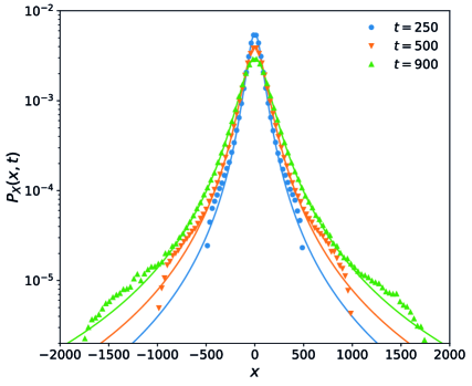
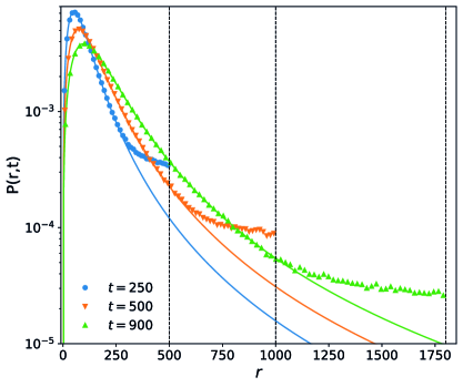
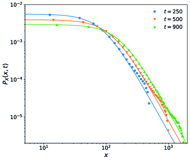
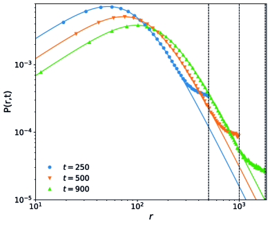
Figure 1: Superstatistical APP model. Top row: For different times we compare the analytic solution (solid lines) with simulations results (dots) for the marginal PDF (20) (left) and the radial PDF (19) (right). Parameters: $v_{0}=2$, $D_{\star}=1$, with time step $dt=10^{-2}$ and number of simulated trajectories $M=10^{5}$. Bottom row: log-log plots of the same cases. The dashed lines in the right panels indicate the maximal distance a particle with speed $v_{0}$ can travel without any directional changes.

The first radial moment of the PDF (19) is defined as $\langle r(t)\rangle=\int_{0}^{\infty}rP(r,t)dr$, and we obtain

$$\langle r(t)\rangle=\frac{\pi}{2}\sqrt{\frac{2v_{0}^{4}}{D_{\star}}}t^{1/2}.$$ (23)

The second moment $\langle r^{2}(t)\rangle$ diverges, as $\lim_{r\rightarrow\infty}r^{2}P(r,t)=1/r$, whose indefinite integral is the natural logarithm and is therefore not defined. This is rather different to the analogous superstatistical approach for passive particles, where the MSD is the same as in the Brownian case, only the single-particle diffusivity being replaced by the effective diffusivity of the ensemble [51], see equation (11).

A common way to evaluate the displacement in the case of distributions with non-definite second moments is to introduce the quantile $p$ and the respective horizon $R_{p}(t)$ such that

$$\int_{0}^{R_{p}(t)}P(r,t)dr=p<1,$$ (24)

which quantifies the advancement of the diffusion front without the need to compute the MSD. To compute $R_{p}(t)$ we rewrite (24) such that

$$\int_{0}^{R_{p}(t)}\frac{D_{\star}}{v_{0}^{4}t\left(\frac{D_{\star}}{2v_{0}^{4}}\frac{r^{2}}{t}+1\right)^{2}}rdr=\int_{0}^{D_{\star}R_{p}^{2}(t)/2v_{0}^{4}t}\frac{1}{(1+y^{2})}dy=p,$$ (25)

where $y=D_{\star}r^{2}/(2v_{0}^{4}t)$. The result is

$$R_{p}(t)=t^{1/2}\sqrt{\left(\frac{p}{1-p}\right)\frac{2v_{0}^{4}}{D_{\star}}},$$ (26)

exhibiting a square root scaling of the horizon, similar to normal diffusion and despite the infinite MSD. In figure 2 we see excellent agreement of the analytic form (26) for $R_{p}(t)$ with the simulations.

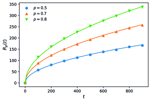
Figure 2: $R_{p}(t)$ from numerical simulations (symbols) compared to the analytic expression (26) for several values of the probability $p$. Parameters: $v_{0}=2$, $D_{\star}=1$, $dt=10^{-2}$, and number of simulated trajectories $M=10^{5}$.

The square-root scaling for $R_{p}(t)$ encountered here reminds of the results obtained from superstatistics as applied to passive particles, where the MSD is shown to retain a linear scaling in time [81], which matches various experimental results.

3.1.2 ABP case.

In the ABP model both translational and rotational diffusivity coefficients influence the particle motion. Considering purely thermal fluctuations and spherical particles, following the Stokes-Einstein relation into the expression (9) for $D^{\prime}_{\mathrm{eff}}$ produces $D^{\prime}_{\mathrm{eff}}=D_{T}+a/D_{T}$, with $a=2R^{2}v_{0}^{2}$, where $R$ is the particle radius [88, 29]. This case was analysed in [82]. Coupling the two degrees of freedom by enforcing the Stokes-Einstein relation may unduly restrict the scope of our study to spherical active agents exclusively undergoing passive, thermal fluctuations. As we are dealing with a far-from-equilibrium system, often also with non-spherical particles, we will consider the case when $D_{R}$ and $D_{T}$ are unrelated. In particular, we keep $D_{T}$ fixed, while $D_{R}$ is varied exponentially, $p(D_{R})=(1/D_{R\star})\exp(-D_{R}/D_{R\star})$, across the ensemble.

The superstatistical displacement PDF for an exponential rotational diffusivity-PDF is then generally given by the integral

$$P(\mathbf{r},t) = \frac{1}{4\pi D_{R\star}t}\int_{0}^{\infty}\frac{1}{D_{T}+v_{0}^{2}/2D_{R}}\exp\left(-\frac{\mathbf{r}^{2}}{4(D_{T}+v_{0}^{2}/2D_{R})t}\right)$$ (27)

$$\times\exp\left(-\frac{D_{R}}{D_{R\star}}\right)dD_{R}.$$

When we assume that the translational diffusivity is much smaller than the active propulsion term, $D_{T}\ll v_{0}^{2}/2D_{R\star}$, which appears a reasonable assumption for propulsion-dominated active transport, the above integral has the same form as (17), the only difference being the specific $v_{0}$ dependency ($v_{0}^{2}$ instead of $v_{0}^{4}$ in (17)). We therefore find

$$P(\mathbf{r},t)=\frac{1}{D_{R\star}}\frac{1}{2\pi v_{0}^{2}t}\int_{0}^{\infty}D_{R}\exp{(-aD_{R})}dD_{R},$$ (28)

where $a=r^{2}/2v_{0}^{2}t+1/D_{R\star}$. Following the same procedure as above we then get the radial and marginal PDFs,

$$P(r,t) = \frac{4rv_{0}^{2}t}{D_{R\star}\left(r^{2}+2v_{0}^{2}t/D_{R\star}\right)^{2}},$$ (29)

$$P_{X}(x,t) = \frac{v_{0}^{2}t}{D_{R\star}\left(x^{2}+2v_{0}^{2}t/D_{R\star}\right)^{3/2}}.$$ (30)

The propagation of the diffusion front for $D_{T}=0$ is obtained analogously, producing

$$R_{p}(t)=t^{1/2}\sqrt{\left(\frac{p}{1-p}\right)\frac{2v_{0}^{2}}{D_{R\star}}}.$$ (31)

For both marginal and radial PDFs, figure 3 shows the comparison between the analytic expressions (29) and (30) and stochastic simulations (based on equations (6) and (7)) of $M=10^{5}$ noise realisations obtained through an Euler-Maruyama integration scheme with a time step $\delta t=10^{-2}$. Results from simulations including translational diffusion ($D_{T}=1$ in dimensionless units) are also shown. One can observe that the shape of the PDFs remains very similar to the Cauchy-type distributions for $D_{T}=0$, with a rounder cusp for $P_{X}(x,t)$ and $P(r,t)$ peaking for slightly higher values. This simply indicates a tendency for slightly higher displacements for higher translational diffusivity, while the general behaviour essentially remains the same. The cutoff at $r_{max}=v_{0}t$ is now less abrupt due to the presence of finite translational diffusion. Generally, we observe a slight shift towards higher displacements between simulations and our approximate analytical solution, due to the fact that we neglected the translational noise in the analytical solutions of the ABP model. The agreement between the analytical and numerical solutions is nevertheless good, especially for short and intermediate $x,r$.

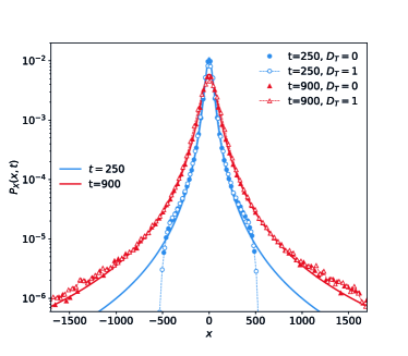
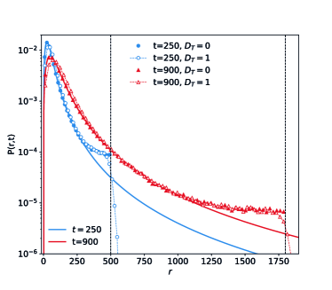
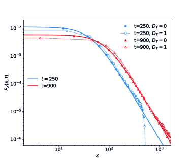
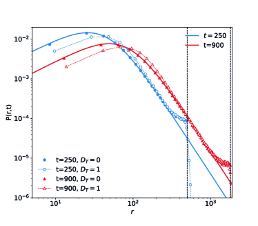
Figure 3: Radial and marginal displacement PDFs for an exponential superstatistical diffusivity-PDF in the minimal ABP model at different times. Analytical results (solid lines) and simulations (symbols) are shown for the $x$-marginal displacement PDF (20) (left) and for the radial PDF (19) (right). Parameters: $v_{0}=2$, $D_{R\star}=1$, $\delta t=10^{-2}$, and number of simulated trajectories $M=10^{5}$. The thin black line serves as a guide for the eye. Bottom row: Same as top row but on log-log scale. Dashed vertical lines in the right panels show the maximal distance $v_{0}t$ travelled ballistically by a particle of constant speed $v_{0}$.

Cauchy-type displacement PDFs, with fat tails and infinite second moments were therefore obtained for an exponential distribution of the rotational diffusivities in both models of active motion discussed here. This fact is in striking contrast to superstatistical and diffusing diffusivity models for purely passive diffusion, in which exponential diffusivity-PDFs effect exponential displacement PDFs (at short times for the case of diffusing diffusivity dynamics) [51]. The occurrence of fat-tailed displacement PDFs from such a quite narrow, exponential diffusivity-PDF is an interesting feature of the active motion models. While in real systems such Cauchy-type shapes may be obscured by finite size effects and other factors such as heterogeneity and/or noise, it should be worthwhile comparing measured displacement PDFs to these "exotic" shapes.

3.2 Distribution of speeds

A heterogeneous population of bacteria, amoeba, insects, etc., will always be characterised by a variety of shapes, sizes, persistence times, and speeds. We here consider superstatistical distributions of speeds, in an "inverse engineering" approach. Namely, we aim at deriving a specific speed-PDF in order to obtain an exponential displacement PDF. Specifically, in a study of the individual motion of social amoeba of the kind dictyostelium discoideum it was shown that the displacement PDF at longer lag times converges to an exponential shape [79], whereas it would be expected to converge to a Gaussian shape for the case of fixed speeds. In the experiment, the marginal PDFs are fitted with stretched Gaussian functions of the shape

$$P(x,t)\propto\exp{(-a|x|^{b})},$$ (32)

where the stretching exponent $b$ is shown to decrease from around 1.2 to a value close to unity for increasing lag times [79]. This may indicate that the Laplace distribution represents the long-time limit of this system and thus intrinsic properties of the dictyostelium population.

3.2.1 APP case: Weibull speed-PDF.

As a starting point we require a bivariate Laplace-shaped displacement PDF, whose marginal in $x$-direction reads

$$P_{X}(x,t)=\frac{1}{\sqrt{4D_{\mathrm{eff}}^{\star}t}}\exp\left(-\frac{|x|}{\sqrt{D_{\mathrm{eff}}^{\star}t}}\right),$$ (33)

which we know arises from an exponential distribution of typical value $D_{\mathrm{eff}}^{\star}$ for the effective diffusivity $D_{\mathrm{eff}}$. In the APP case we showed that $v=(2DD_{\mathrm{eff}})^{1/4}$, and thus $p(v)=p(D_{\mathrm{eff}})|dD_{\mathrm{eff}}/dv|$ as $D_{\mathrm{eff}}$ is a monotonous function of $v>0$. Thus, requiring the exponential form $p(D_{\mathrm{eff}})=(D_{\mathrm{eff}}^{\star})^{-1}\exp(-D_{\mathrm{eff}}/D_{\mathrm{eff}}^{\star})$, we find the corresponding speed-PDF

$$p(v)=\frac{4v^{3}}{2DD_{\mathrm{eff}}^{\star}}\exp\left(-\frac{v^{4}}{2DD_{\mathrm{eff}}^{\star}}\right).$$ (34)

This form for $p(v)$ corresponds to a Weibull distribution of the general shape

$$f_{W}(x;k,\lambda)=\frac{k}{\lambda}\left(\frac{x}{\lambda}\right)^{k-1}e^{-(x/\lambda)^{k}},$$ (35)

which in turn is a special case of the generalised gamma distribution

$$f_{G}(x;k,\theta,\beta)=\frac{\beta}{\Gamma(k)\theta}\left(\frac{x}{\theta}\right)^{k\beta-1}e^{-(x/\theta)^{\beta}}.$$ (36)

Both are valid for for $x\geq 0$ and vanish for $x<0$.

Stochastic simulations based on equation (1) were run with parameters $\delta t=10^{-2}$, $D_{\mathrm{eff}}^{\star}=8$, and $D=0.4$, for $M=10^{5}$ realisations. In figure 4 (left) we show a comparison between the Laplace distribution (33) and the numerically obtained PDFs, demonstrating very good agreement at longer time scales (we show $t=20$, $100$, and $300$). The MSD remains exactly the same as for the fixed-speed APP model, if we choose the propulsion speed to be $v_{0}=(2DD_{\mathrm{eff}}^{\star})^{1/4}$. Thus, the MSD is ballistic at short times and linear in the long-time limit. Additional PDFs for different times $t$ are plotted in figure 4 (right), where it can be seen that the PDF gradually approaches the expected Laplace-like shape at longer times.

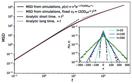
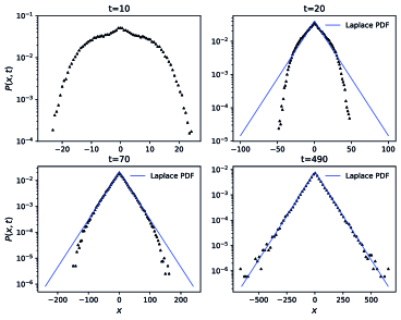
Figure 4: Left: MSD and PDFs (inset) for the APP model with the Weibull-shaped speed-PDF (34). The MSD in the fixed-speed case is also shown by the dashed red line. The blue, cyan, and green solid lines (inset) indicate Laplace PDFs. Right: Marginal displacement PDF in $x$-direction, for additional times. The solid blue lines indicate Laplace-shaped PDFs. In both panels, we chose $D_{\mathrm{eff}}^{\star}=8$, $D=0.2$, $\delta t=10^{-2}$, and the number of trajectories $M=10^{5}$.

The generalised gamma distribution was in fact shown to describe the speed distribution of Protozoa cells [23] as well as the above mentioned dictyostelium [79]. The exponents determined from experiment are, however, quite different from those of a Weibull distribution, with $\theta=\beta\approx 1$ and $k\approx 2$ resulting in $p_{\mathrm{exp}}(v)\approx v\exp{(-v)}$. The displacement PDFs obtained from this experimental speed distribution or from a Rayleigh distribution (in general, from any generalised gamma distribution) can again be derived with a similar method to that of superstatistics. Namely, using the generalised Gamma distribution (36) for the speed and with $v=(DD_{\mathrm{eff}})^{1/4}$, we find

$$p(D_{\mathrm{eff}})=\frac{\beta(2DD_{\mathrm{eff}})^{k\beta/4}}{4\theta^{k\beta}\Gamma(k)D_{\mathrm{eff}}}\exp\left(-\left[\frac{(2DD_{\mathrm{eff}})^{1/4}}{\theta}\right]^{\beta}\right).$$ (37)

We then insert this form into the superstatistical formulation

$$P(\mathbf{r},t)=\frac{1}{4\pi t}\int_{0}^{\infty}\frac{1}{D_{\mathrm{eff}}}p(D_{\mathrm{eff}})\exp\left({-\frac{\mathbf{r}^{2}}{4D_{\mathrm{eff}}t}}\right)dD_{\mathrm{eff}}.$$ (38)

This integral can be solved using Fox $H$-functions (see C), leading to the expression

$$P(\mathbf{r},t)=\frac{1}{4\pi t}\frac{1}{\Gamma(k)}\frac{(2D)^{1-4/\beta}}{\theta^{4-\beta}}H_{0,2}^{2,0}\left[\frac{2D\mathbf{r}^{2}}{\theta^{4}4t}\left|\begin{array}[]{l}\rule{34.14322pt}{0.28436pt}\\ (k-4/\beta,4\beta),(0,1)\end{array}\right.\right].$$ (39)

For the marginal PDF in $x$, we find

$$P_{X}(x,t)=\frac{a^{l-1}}{\sqrt{4\pi t}\Gamma(k)}H_{0,2}^{2,0}\left[b\left|\begin{array}[]{l}\rule{34.14322pt}{0.28436pt}\\ (k-l+\frac{1}{2},l),(0,1)\end{array}\right.\right]$$ (40)

The large-displacement asymptote of the marginal $P_{X}(x,t)$ can be obtained explicitly, yielding

$$P_{X}(x,t)\simeq\frac{a^{l-1}}{\sqrt{4\pi t}\Gamma(k)}\left(\frac{a^{l}x^{2}}{4t}\right)^{(k-l)/(1+l)}\exp\left(-\frac{1+l}{l^{l/(1+l)}}\left(\frac{a^{l}x^{2}}{4t}\right)^{1/(1+l)}\right),$$ (41)

for $(a^{l}x^{2}/4t)\to\infty$, with $a=(2D)^{\beta/4}/\theta^{\beta}$ and $l=\beta/4$, and where $\theta$, and $\beta$ are the parameters of the Gamma distribution. Here the symbol $\simeq$ signifies that the expansion is known up to a ("scaling") factor of the order of unity. Additional details of the derivation are presented in C. Figure 5 compares the PDFs obtained from simulations with the analytic asymptotic results. In particular, we see that the effective diffusivity-PDF corresponding to the the experimentally observed speed PDF $p(v)\approx v\exp(-v)$ in [79] (green line), produces a marginal PDF with a sharper cusp and significantly broader tails than a Laplace PDF. We will show that the sought-after consistency between the experimental speed- and displacement-PDFs can be recovered in the ABP model.

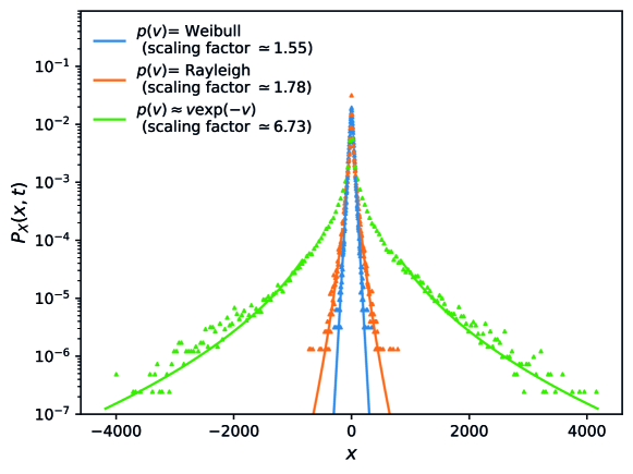
Figure 5: Marginal PDF $P_{X}(x,t)$ for various speed PDFs in the APP model at time $t=490$. Analytic large-displacement asymptotics as obtained from (41) (solid lines) and comparison with stochastic simulations (triangles) with various distributions of the speed $v_{0}$. For all distributions, $D=0.4$, the number of trajectories is $M=10^{5}$, $\delta t=10^{-2}$. Based on equation (37) we use the fitted distributions from [79] with $k=2$, $\theta=\beta=1$; a Rayleigh distribution with $k=1$, $\beta=2$, $\theta=1$; and a Weibull distribution with $k=1$, $\beta=4$, $\theta=1$. The "scaling factor" listed in the figure is needed to account for the constant factor, that is unknown in the expansion (41).

3.2.2 ABP case: Rayleigh PDF.

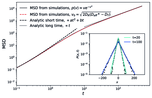
Figure 6: MSD and PDFs for the ABP model in the case of a Rayleigh speed-PDF. The MSD in the case with fixed speed $v_{0}=\langle v\rangle$ equalling the mean of the speed of the Rayleigh PDF is also shown (dashed red line). The solid lines (inset) indicate exponential PDFs, while the dashed line is a best fit to the shape $A\exp{(|x|^{\alpha}/b)}$, $\alpha\simeq 1.21$. Here $D_{\mathrm{eff}}^{\star}=8$, $D_{R}=0.4$, $D_{T}=0.2$, and $\delta t=10^{-2}$, for $M=10^{5}$ trajectories.

We now assume that the long-time diffusivity $D^{\prime}_{\mathrm{eff}}=D_{T}+v_{0}^{2}/2D_{R}$ of the ABP model follows the exponential distribution $p(D^{\prime}_{\mathrm{eff}})\approx(1/D_{\mathrm{eff}}^{\star})\exp{(-D^{\prime}_{\mathrm{eff}}/D_{\mathrm{eff}}^{\star})}$, such that the speed-PDF has the Rayleigh shape

$$p(v)\approx\frac{v}{D_{R}D_{\mathrm{eff}}^{\star}}\exp{\left(\frac{-v^{2}}{2D_{R}D_{\mathrm{eff}}^{\star}}\right)}.$$ (42)

This form also corresponds to the Maxwellian distribution of velocities, that was found by Okubo and Chiang [100] for the speed distribution of flying insects. We compare this result to stochastic simulations of equations (6) and (7) with parameters $\delta t=10^{-2}$, $D_{\mathrm{eff}}^{\star}=8$, $D_{R}=0.4$, and $D_{T}=0.2$, for $M=10^{5}$ noise realisations in figure 6. The MSD obtained from simulations with this initial distribution remains unchanged from the fixed-$v$ case. The PDFs shown in figure 6 (additional times are shown in figure 7, left) evolve from having a close-to-Gaussian shape at short lag times to a distribution that nicely matches the Laplace distribution (33) at long lag times. This corresponds quite well to the experimental findings in [79], where the fitted stretching exponent $b$ (compare (32)) decreases from $b\approx 1.2$ to a value close to unity at longer lag times.

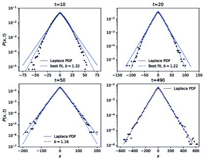
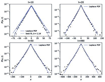
Figure 7: Marginal displacement PDFs in $x$-direction from simulations in the ABP model for a Rayleigh speed-PDF (left) and the experimentally fitted speed-PDF (right). The solid lines indicate an exponential PDF while the dashed lines are best fits for functions of the type $A\exp(-|x|^{b}/c)$. The parameters are $D_{\mathrm{eff}}^{\star}=8$, $D_{R}=0.4$, $D_{T}=0.2$, $\delta t=0.01$, and the number of trajectories is $M=10^{5}$.

In the experimental study of dictyostelium [79] it was, however, shown that the experimental speed-PDF grew faster at small speeds and had more pronounced tails at high speeds. Instead of the Rayleigh distribution the generalised two-parameter Gamma distribution

$$p_{\mathrm{exp}}(v)=\frac{\gamma}{\Gamma(\varepsilon+1/\gamma)}v^{\varepsilon\gamma}\exp\left(-v^{\gamma}\right)$$ (43)

with $\gamma\approx 1$ and $\varepsilon\approx 1$, i.e., an approximately exponential speed-PDF, was shown to provide an excellent fit. The analytic expression of the large-displacement asymptotes for $P(\mathbf{r},t)$ and $P_{X}(x,t)$ can again be obtained via Fox $H$-functions, see C. In particular, the marginal PDF corresponding to the speed PDF (43) fitted to the experimental data in [79]) can, in the asymptotic limit, be written as

$$P_{X}(x,t)\simeq\frac{1}{\sqrt{4\pi t}}\frac{1}{\Gamma(2)}\frac{\sqrt{2D_{R}}}{\theta}\exp{\left(-3\times 2^{-2/3}\left(\frac{\sqrt{2D_{R}}x^{2}}{4t\theta}\right)^{1/3}\right)},$$ (44)

for $D_{R}x^{2}/(2t\theta^{2})\to\infty$. Figure 8 shows good agreement between the simulations and the analytic large-displacement asymptotes. We see how this speed PDF actually leads to the asymptote $P(x,t)\propto\exp{(-ax^{2/3})}$. The comparison between the displacement PDF obtained from simulations with this speed PDF (43) and a Laplace PDF nonetheless shows that for intermediate times, both distributions actually match very well.

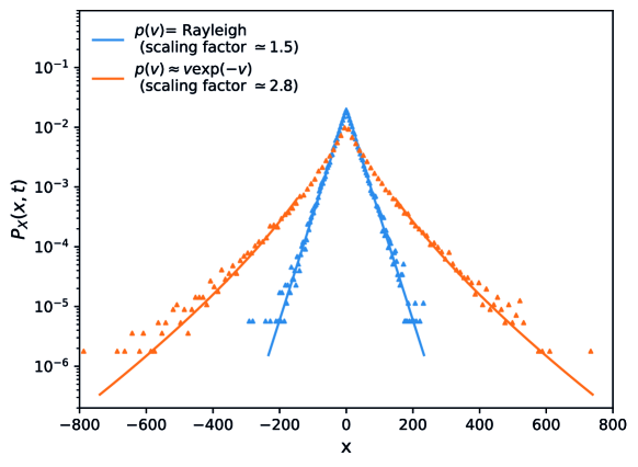
Figure 8: Analytic large-displacement asymptotics for the ABP model as obtained from (44) (orange line) and (112) (blue line) and comparison with numerics (triangles), for two PDFs of the initial speed (both with $D_{R}=0.4$, $D_{T}=0$, number of trajectories $M=10^{5}$, and $\delta t=10^{-2}$). PDF with $k=2$, $\theta=\beta=1$; Rayleigh distribution with $k=1$, $\beta=2$, $\theta=1$. The "scaling factor" listed in the figure is needed to account for the constant factor, that is unknown in the expansion (41).

We point out the almost perfect agreement between the marginal displacement PDFs shown for the lag time $t=20$, at which the MSD crosses over between the short-time ballistic and the linear long-time regime, as seen in figure 6. We also note that the displacement PDFs obtained at shorter lag times can also be fitted rather well with functions of the form (32), with $1<b<2$, despite some difference at smaller displacements. Despite the simple assumptions of our model in combination with the experimental speed-PDF the agreement with the experimentally observed displacement PDF at various times is remarkable and demonstrates that the ABP model provides an adequate model for the dictyostelium motion based on the current data. In particular, the agreement is much better than for the APP model.

4 Conclusion

Common models for active stochastic motion are characterised by some specific correlation time, beyond which the motion converges to normal Brownian motion with a Gaussian displacement PDF and an MSD, that is linear in time and has an effective diffusion coefficient, in which the typical particle speed and the correlation time enter. Following reports of non-Gaussian displacement PDFs, we here developed superstatistical extensions of two active particle models: One is the APP model including passive-noise. This model is mainly useful for the description of particles with small damping coefficients, for instance, insects or birds. The other is the ABP model with active fluctuations. For both models we considered distributions in their diffusion coefficients and speeds. For living creatures such variations can be thought of as physiologically given, such that random parameters occur even in an homogeneous environment. In this sense the phenomenon of non-Gaussian active particles is similar to "ensembles" of non-ideal, passive tracer particles with a significant distribution of particle sizes or shapes.

For distributed diffusivities we found that an exponential distribution of particle diffusivities in the APP model give rise to a Cauchy-type displacement PDF, for which we also calculated the diffusion fronts. A similar result was obtained for the ABP case with an exponential diffusivity-PDF. Thus, active particle models behave very differently from passive particles, for which an exponential diffusivity PDF effects exponential tails of the displacement PDF. For the analysis of the distribution of speeds we required that the asymptotic displacement PDF follows a Laplace PDF. To achieve this, in the APP model we employed a Weibull speed-PDF. We also presented the results for a more versatile generalised gamma distribution. For the ABP model we discussed a Rayleigh speed-distribution and a generalised gamma distribution. It turns out that the description in terms of the superstatistical ABP model with random speeds selected from the experimentally measured speed-PDF provides a very nice description of the experimentally determined marginal displacement PDF in $x$-direction. The superstatistical ABP model driven by active fluctuations thus provides a consistent link between the experimentally determined displacement- and speed-PDFs.

The diffusion of active particles in evolving heterogeneous environments was recently investigated in [82] through the implementation of the "diffusing diffusivity" mechanism, according to which the diffusivity of each particle is taken as a random variable evolving through time as a stationary stochastic process, e.g., the Ornstein-Uhlenbeck process. The obtained results include a non-Gaussian displacement PDF at time scales shorter than the correlation time of the auxiliary diffusivity process. At long times, this model shows a convergence to a Gaussian profile with an effective diffusivity. It is thus different from our superstatistical model, in which, in an heterogeneous environment, the parameter randomness is due to individual physiology, and the non-Gaussianity persists in the long time limit. The latter case corresponds to the experimental results for dictyostelium [79] and nematodes [81].

Active baths, i.e., an environment made up of a great number of active particles, are of interest for both their role in concrete biological or engineering systems and their physically remarkable behaviour due to co-operativity effects [101]. Such experiments found interesting diffusion behaviour for the passive particles, some of them exhibiting exponential tails [78]. It will be interesting to study the emerging co-operative dynamics of baths of non-identical particles with superstatistically distributed parameters.

Following the favourable comparison of our results with dictyostelium cells analysed here, it could be interesting to see how other motile-cellular systems behave statistically, e.g., acanthamoeba cells, whose intracellular motion in supercrowded cells was found to be strongly superdiffusive [102], and who also perform superdiffusive active motion of the entire cell [103]. We could also think of applying such modelling to larger animals, such as the motion of birds such as kites and storks [104]. Finally, extensions to intermittent dynamics such as run-and-tumble models are possible [105].

Appendix A Probability density function of the director angle $\phi(t)$

We here derive the PDF for the director angle $\phi(t)$ needed to determine the MSD in B. Let $\phi$ be a $2\pi$-periodic Wiener process that follows the Langevin equation

$$\frac{d\phi(t)}{dt}=\frac{1}{v_{0}}\sqrt{2D}\xi(t),$$ (45)

or, equivalently, the Fokker-Planck equation

$$\frac{\partial P(\phi,t|\phi_{0},t_{0})}{\partial t}=\frac{D}{v_{0}^{2}}\frac{\partial^{2}P(\phi,t|\phi_{0},t_{0})}{\partial^{2}\phi}.$$ (46)

Let us now retrieve its PDF $P(\phi,t|\phi_{0})$ for a given initial condition $\phi_{0}$. We use $a=D/v_{0}^{2}$ in the following, and set $t_{0}=0$. One knows that $P(\phi,t=0)=\delta(\phi-\phi_{0})$ and that $0\leq\phi\leq 2\pi$. We can write the expansion

$$P(\phi,t|\phi_{0})=\sum_{n=-\infty}^{\infty}V_{n}(t)e^{in\phi}\leavevmode\nobreak\ ,$$ (47)

and therefore know that

$$\delta(\phi-\phi_{0})=\sum_{n=-\infty}^{\infty}V_{n}(0)e^{in\phi}.$$ (48)

Multiplying on both sides of equation (48) with $\int_{0}^{2\phi}d\phi e^{-im\phi}$, $m\in\mathbb{Z}$, we eventually get that

$$\int_{0}^{2\phi}\delta(\phi-\phi_{0})e^{-im\phi}d\phi=\sum_{n=-\infty}^{\infty}V_{n}(0)\int_{0}^{2\phi}e^{i(n-m)\phi}d\phi,$$ (49)

where the right-hand term is non-zero only for $n=m$. Thus,

$$V_{n}(0)=\frac{e^{-in\phi_{0}}}{2\pi}.$$ (50)

Now we can plug expression (47) into (46) and get a differential equations for the coefficients $V_{n}(t)$, such that

$$\sum_{n=-\infty}^{\infty}\frac{dV_{n}}{dt}e^{in\phi}=-a\sum_{n=-\infty}^{\infty}V_{n}(t)e^{in\phi},$$ (51)

which yields, after repeating the procedure leading to equation (49),

$$2\pi\frac{dV_{m}}{dt}=-2\pi aV_{m}(t)m^{2}.$$ (52)

The differential equation (52) is easily solved, and we get

$$V_{n}(t)=V_{n}(0)e^{-n^{2}at}.$$ (53)

Knowing $V_{n}(0)$, we can thus retrieve the expression $P(\phi,t|\phi_{0})$,

$$P(\phi,t|\phi_{0}) = \frac{1}{2\pi}\sum_{n=-\infty}^{\infty}e^{(in(\phi-\phi_{0}))}e^{-n^{2}at},$$ (54a)

$$= \frac{1}{2\pi}+\frac{1}{2\pi}\sum_{n=-\infty}^{-1}e^{in(\phi-\phi_{0})}e^{-n^{2}at}+\frac{1}{2\pi}\sum_{n=1}^{\infty}e^{(in(\phi-\phi_{0}))}e^{-n^{2}at},$$ (54b)

$$= \frac{1}{2\pi}+\frac{1}{2\pi}\sum_{n=-\infty}^{-1}\left(e^{in(\phi-\phi_{0})}+e^{-in(\phi-\phi_{0})}\right)e^{-n^{2}at},$$ (54c)

thus eventually yielding

$$P(\phi,t|\phi_{0})=\frac{1}{\pi}\left(\frac{1}{2}+\sum_{n=1}^{\infty}\cos n(\phi-\phi_{0})\exp{\left(-n^{2}\frac{D}{v_{0}^{2}}t\right)}\right).$$ (55)

This formula is used below in B.

Appendix B Derivation of the MSD of the Mikhailov-Meinköhn model

The APP model was introduced in in [89]. The expression of the MSD is obtained from the identity $\mathbf{r}(t)=\int_{0}^{t}\mathbf{v}(t^{\prime})dt^{\prime}$, knowing that $\mathbf{v}(t)=v_{0}\mathbf{e_{v}}$, with $\mathbf{e_{v}}=(\cos\phi,\sin\phi)$. This leads to

$$\langle\mathbf{r}^{2}(t)\rangle = \langle(v_{0}\int_{0}^{t}\mathbf{e_{v}}(t_{1})dt_{1})(v_{0}\int_{0}^{t}\mathbf{e_{v}}(t_{2})dt_{2})\rangle,$$ (56)

$$= v_{0}^{2}\int_{0}^{t}\int_{0}^{t}\langle\cos\phi(t^{\prime})\rangle dt_{1}dt_{2}.$$ (57)

Here $\phi$ is the angle between the direction of motion of the active agent at $t=t_{1}$ and at $t=t_{2}$, and $t^{\prime}$ is the time difference, either $t_{1}-t_{2}$ or $t_{2}-t_{1}$. Indeed, the probability density of the Wiener process $\phi$ is only defined for positive times, therefore $t^{\prime}>0$. This means that $t^{\prime}=t_{2}-t_{1}$ for $t_{2}>t_{1}$ and $t^{\prime}=t_{1}-t_{2}$ for $t_{1}>t_{2}$. We rewrite the integral as

$$\langle\mathbf{r}^{2}(t)\rangle=v_{0}^{2}\int_{0}^{t}\int_{0}^{t_{1}}\langle\cos\phi(t_{1}-t_{2})\rangle dt_{1}dt_{2}+v_{0}^{2}\int_{0}^{t}\int_{t_{1}}^{t}\langle\cos\phi(t_{2}-t_{1})\rangle dt_{1}dt_{2}.$$ (58)

Changing the order of integration in the second term and using the fact that the cosine is an even function, we get

$$\langle\mathbf{r}^{2}(t)\rangle=2v_{0}^{2}\int_{0}^{t}\int_{0}^{t_{1}}\langle\cos\phi(t_{1}-t_{2})\rangle dt_{1}dt_{2}.$$ (59)

To compute the quantity $\langle\cos{\phi(t^{\prime})}\rangle$ we use the property that

$$\langle\cos\phi(t^{\prime})\rangle=\int_{0}^{2\pi}\cos\phi(t^{\prime})P(\phi,t^{\prime})d\phi,$$ (60)

with

$$P(\phi,t^{\prime})=\int_{-\pi}^{\pi}P(\phi,t^{\prime}|\phi_{0})P(\phi_{0})d\phi_{0}.$$ (61)

We further note that $\phi$ is a $2\pi$-periodic Wiener process, which is distributed according to (55). Posing a delta distribution for $\phi_{0}$, $P(\phi_{0})=\delta(\phi_{0})$ (it has to be precisely this distribution as the angles are necessarily the same for $\phi(t^{\prime}=0)=\phi(t_{1}=t_{2})$) we can then compute the ensemble average

$$\langle\cos\phi(t^{\prime})\rangle=\frac{1}{\pi}\left[\frac{1}{2}\int_{0}^{2\pi}\cos\phi d\phi+\int_{0}^{2\pi}\sum_{n=1}^{\infty}\cos\phi\cos n\phi\exp\left(-n\frac{D}{v_{0}^{2}}t^{\prime}\right)d\phi\right].$$ (62)

The term on the left cancels and $\cos\phi\cos n\phi=\frac{1}{2}(\cos(n+1)\phi+\cos(n-1)\phi)$, whose integral from 0 to $2\pi$ is always 0, except for $n=1$, which then yields $\pi$. We thus find

$$\langle\cos\phi(t^{\prime})\rangle=\exp\left(-\frac{D}{v_{0}^{2}}t^{\prime}\right),$$ (63)

which we may now plug into equation (59). We calculate the double integral,

$$\int_{0}^{t}\int_{0}^{t_{1}}\langle\cos\phi(t_{1}-t_{2})\rangle dt_{1}dt_{2}=\int_{0}^{t}\int_{0}^{t_{1}}\exp\left(\frac{D}{v_{0}^{2}}(t_{2}-t_{1})\right)dt_{1}dt_{2},$$ (64)

$$= \int_{0}^{t}\left(\frac{v_{0}^{2}}{D}\right)\left(1-\exp\left(-\frac{D}{v_{0}^{2}}t_{1}\right)\right)dt_{1},$$

$$= \frac{v_{0}^{2}}{D}\left[\int_{0}^{t}dt_{1}-\int_{0}^{t}\exp\left(-\frac{D}{v_{0}^{2}}t_{1}\right)dt_{1}\right],$$

$$= \frac{v_{0}^{2}}{D}t-\frac{v_{0}^{2}}{D}\left(\frac{-v_{0}^{2}}{D}\right)\left(\exp\left(-\frac{D}{v_{0}^{2}}t_{1}\right)-1\right),$$

$$= \frac{v_{0}^{2}}{D}t+\frac{v_{0}^{4}}{D^{2}}\left(\exp\left(-\frac{D}{v_{0}^{2}}t\right)-1\right).$$

We then obtain the final expression

$$\langle\mathbf{r}^{2}(t)\rangle=\frac{2v_{0}^{4}}{D}t+\frac{2v_{0}^{6}}{D^{2}}\left(\exp\left(-\frac{D}{v_{0}^{2}}t\right)-1\right).$$ (65)

This result differs slightly from that reported in [89] (in their notation $D=\sigma/m^{2})$, which reads

$$\langle\mathbf{r}^{2}(t)\rangle=\frac{2v_{0}^{4}m^{2}t}{\sigma}+\frac{v_{0}^{6}m^{4}}{\sigma^{2}}\left(\exp\left(\frac{-2\sigma t}{m^{2}v_{0}^{2}}\right)-1\right).$$ (66)

Thus, equation (65) has an extra factor of 2 in front of the $v_{0}^{6}$-term and a missing factor of 2 in the exponential, as compared to results in [89]. However, both results have the same long-time limit, $D_{\mathrm{eff}}=\frac{v_{0}^{4}}{2D}$. In contrast, our corrected result has the short time limit $v_{0}^{2}t^{2}$ (instead of $2v_{0}^{2}t^{2}$).

Appendix C Applications of the Fox $H$-function technique and asymptotic expansions

We here provide details on the application of the Fox $H$-function technique to calculate the integrals of the main part, for both the APP and ABP cases.

C.1 Active particle with passive-noise case

We start with equation

$$P(\mathbf{r},t)=\frac{1}{4\pi t}\int_{0}^{\infty}\frac{1}{D_{\mathrm{eff}}}p(D_{\mathrm{eff}})\exp\left(-\frac{\mathbf{r}^{2}}{4D_{\mathrm{eff}}t}\right)dD_{\mathrm{eff}},$$ (67)

for which we know that (where $k$, $\beta$, and $\gamma$ are the parameters of the generalised Gamma distribution (37))

$$p(D_{\mathrm{eff}};k,\theta,\beta)=\frac{\beta(2DD_{\mathrm{eff}})^{1/4}}{4\theta\Gamma(k)D_{\mathrm{eff}}}\left(\frac{(2DD_{\mathrm{eff}})^{1/4}}{\theta}\right)^{k\beta-1}e^{-((2DD_{\mathrm{eff}})^{1/4}/\theta)^{\beta}}.$$ (68)

We introduce the abbreviations

$$a = \frac{(2D)^{\beta/4}}{\theta^{\beta}},$$ (69)

$$s = aD_{\mathrm{eff}}^{\beta/4},$$ (70)

$$l = \frac{4}{\beta},$$ (71)

$$b = \frac{a^{l}\mathbf{r}^{2}}{4t},$$ (72)

so that we can rewrite and rearrange (67) in the form

$$P(\mathbf{r},t) = \frac{1}{4\pi t}\frac{1}{\Gamma(k)}a^{l-1}\int_{0}^{\infty}s^{k-l-1}\exp{(bs^{-l})}\exp{(-s)}ds.$$ (73)

We now use the property [107] (p.151)

$$e^{-z}=H_{0,1}^{1,0}\left[z\left|\begin{array}[]{l}\rule{34.14322pt}{0.28436pt}\\ (0,1)\end{array}\right.\right],$$ (74)

meaning that (73) can be rewritten as

$$P(\mathbf{r},t)=\frac{a^{l-1}}{4\pi t\Gamma(k)}\int_{0}^{\infty}s^{k-l-1}H_{0,1}^{1,0}\left[bs^{-l}\left[\begin{array}[]{l}\rule{34.14322pt}{0.28436pt}\\ (0,1)\end{array}\right.\right]\exp{(-s)}ds.$$ (75)

We continue by using the identity [107] (p.4 equation (1.2.2))

$$H_{p,q}^{m,n}\left[z\left|\begin{array}[]{l}(a_{p},A_{p})\\ (b_{q},B_{q})\end{array}\right.\right]=H_{q,p}^{n,m}\left[\frac{1}{z}\left|\begin{array}[]{l}(1-b_{q},B_{q})\\ (1-a_{p},A_{p})\end{array}\right.\right],$$ (76)

which in our case leads to

$$H_{0,1}^{1,0}\left[bs^{-l}\left|\begin{array}[]{l}\rule{34.14322pt}{0.28436pt}\\ (0,1)\end{array}\right.\right]=H_{1,0}^{0,1}\left[\frac{s^{l}}{b}\left|\begin{array}[]{l}(1,1)\\ \rule{34.14322pt}{0.28436pt}\end{array}\right.\right].$$ (77)

It can also be shown that (see [108] p.300)

$$\int_{0}^{\infty} x^{\alpha-1}e^{-\sigma x}H_{p,q}^{m,n}\left[wx^{r}\left|\begin{array}[]{l}(a_{p},A_{p})\\ (b_{q},B_{q})\end{array}\right.\right]dx$$ (80)

$$=\sigma^{-\alpha}H_{p+1,q}^{m,n+1}\left[\frac{w}{\sigma^{r}}\left|\begin{array}[]{l}(1-\alpha,r),(a_{p},A_{p})\\ (b_{q},B_{q})\end{array}\right.\right].$$ (83)

Making the appropriate replacements $\alpha=k-l$, $w=1/b$, $r=l$ and $\sigma=1$ we eventually obtain

$$P(\mathbf{r},t) = \frac{a^{l-1}}{4\pi t\Gamma(k)}H_{2,0}^{0,2}\left[\frac{1}{b}\left|\begin{array}[]{l}(1-k+l,l),(1,1)\\ \rule{34.14322pt}{0.28436pt}\end{array}\right.\right]$$ (86)

$$= \frac{a^{l-1}}{4\pi t\Gamma(k)}H_{0,2}^{2,0}\left[b\left|\begin{array}[]{l}\rule{34.14322pt}{0.28436pt}\\ (k-l,l),(0,1)\end{array}\right.\right].$$ (89)

We write (89) explicitly with the parameters given in equations (69) to (72), yielding

$$P(\mathbf{r},t)=\frac{1}{4\pi t\Gamma(k)}\frac{(2D)^{1-4/\beta}}{\theta^{4-\beta}}H_{0,2}^{2,0}\left[\frac{2D\mathbf{r}^{2}}{\theta^{4}4t}\left|\begin{array}[]{l}\rule{34.14322pt}{0.28436pt}\\ (k-4/\beta,4\beta),(0,1)\end{array}\right.\right].$$ (90)

To get the marginal $P_{X}(x,t)$ we write

$$P_{X}(x,t) = \int_{-\infty}^{+\infty}P(x,y,t)dy,$$ (91)

$$= \frac{1}{4\pi t}\int_{-\infty}^{\infty}\int_{0}^{\infty}\frac{1}{D_{\mathrm{eff}}}p(D_{\mathrm{eff}})\exp({-(x^{2}+y^{2})/4D_{\mathrm{eff}}t})dD_{\mathrm{eff}}dy,$$

$$= \frac{1}{4\pi t}\int_{0}^{\infty}\frac{1}{D_{\mathrm{eff}}}p(D_{\mathrm{eff}})\exp({-x^{2}/4D_{\mathrm{eff}}t})dD_{\mathrm{eff}}$$

$$\times\int_{-\infty}^{\infty}\exp({-y^{2}/4D_{\mathrm{eff}}t})dy,$$

which, with the Gaussian integral $\int_{-\infty}^{\infty}e^{-ax^{2}}dx=\sqrt{\frac{\pi}{a}}$, leads to

$$P_{x}(x,t)=\frac{1}{\sqrt{4\pi t}}\int_{0}^{\infty}\frac{1}{\sqrt{D_{\mathrm{eff}}}}p(D_{\mathrm{eff}})\exp({-x^{2}/4D_{\mathrm{eff}}t})dD_{\mathrm{eff}}.$$ (92)

We then establish that

$$P_{X}(x,t)=\frac{a^{l-1}}{\sqrt{4\pi t}\Gamma(k)}\int_{0}^{\infty}s^{k-l-1/2}\exp{(bs^{-l})}\exp{(-s)}ds,$$ (93)

which, using the expressions (76) and (83), and with $\alpha=k-l+1/2$ leads to

$$P_{X}(x,t) = \frac{1}{\sqrt{4\pi t}}\frac{1}{\Gamma(k)}a^{l-1}H_{2,0}^{0,2}\left[\frac{1}{b}\left|\begin{array}[]{l}(\frac{1}{2}-k+l,l),(1,1)\\ \rule{34.14322pt}{0.28436pt}\end{array}\right.\right]$$ (96)

$$= \frac{1}{\sqrt{4\pi t}}\frac{1}{\Gamma(k)}a^{l-1}H_{0,2}^{2,0}\left[b\left|\begin{array}[]{l}\rule{34.14322pt}{0.28436pt}\\ (k-l+\frac{1}{2},l),(0,1)\end{array}\right.\right].$$ (99)

An asymptotic expansion of the previous expression can be found in [109] (p.20, equation (1.108)), which for our special case of the $H$-function with $m=q$ and $n=0$ produces

$$H_{q,0}^{p,q}(z)=\mathcal{O}(z^{(\mathrm{Re}(\delta)+1/2)/\mu})\exp\left(-\mu\beta^{-1/\mu}z^{1/\mu}\right),\quad|z|\to\infty,$$ (100)

where $\delta$, $\mu$, and $\beta$ are parameters related to the parameters $a_{i}$, $A_{i}$, $b_{j}$, $B_{j}$ of the Fox $H$-function (see [109] p.3). In our case, we get, as a functions of the parameters defined above,

$$\beta = l^{l},$$ (101)

$$\mu = 1+l,$$ (102)

$$\delta = k-l-\frac{1}{2}.$$ (103)

Making the appropriate replacements, we may therefore get an asymptotic expression valid for large displacements of the marginal displacement PDF (92), namely,

$$P_{X}(x,t) \simeq \frac{a^{l-1}}{\sqrt{4\pi t}\Gamma(k)}\left(\frac{a^{l}x^{2}}{4t}\right)^{(k-l)/(1+l)}$$ (104)

$$\times\exp\left(-\frac{1+l}{l^{l/(1+l)}}\left(\frac{a^{l}x^{2}}{4t}\right)^{1/(1+l)}\right),\quad\frac{a^{l}x^{2}}{4t}\to\infty.$$

C.2 Active Brownian particles

For the ABP model we follow the same procedure as in the previous section. We point out that we here take $D_{\mathrm{eff}}\simeq v^{2}/2D_{R}$, as the translational diffusivity $D_{T}$ is neglected in this calculation, see the main text. We now have that (with $k$, $\beta$, $\gamma$ as the parameters of the generalised Gamma distribution (37))

$$p(D_{\mathrm{eff}};k,\theta,\beta)=\frac{\beta(2D_{R}D_{\mathrm{eff}})^{1/2}}{2\theta\Gamma(k)D_{\mathrm{eff}}}\left(\frac{(2D_{R}D_{\mathrm{eff}})^{1/2}}{\theta}\right)^{k\beta-1}e^{-((2D_{R}D_{\mathrm{eff}})^{1/2}/\theta)^{\beta}}.$$ (105)

We then introduce the abbreviations

$$a = \frac{(2D_{R})^{\beta/2}}{\theta^{\beta}},$$ (106)

$$s = aD_{\mathrm{eff}}^{\beta/2},$$ (107)

$$l = \frac{2}{\beta},$$ (108)

$$b = \frac{a^{l}\mathbf{r}^{2}}{4t},$$ (109)

The next steps are exactly the same as above in C.1, such that we can directly write

$$P(\mathbf{r},t)=\frac{1}{4\pi t\Gamma(k)}\frac{(2D_{R})^{1-2/\beta}}{\theta^{2-\beta}}H_{0,2}^{2,0}\left[\frac{2D_{R}\mathbf{r}^{2}}{\theta^{2}4t}\left|\begin{array}[]{l}\rule{34.14322pt}{0.28436pt}\\ (k-2/\beta,2\beta),(0,1)\end{array}\right.\right].$$ (110)

For the marginal, we use (104) which for the distribution found experimentally in [79]), where $l=2$ ($\beta=1$) and $k=2$, and find

$$P_{X}(x,t)\simeq\frac{1}{\sqrt{4\pi t}}\frac{1}{\Gamma(2)}\frac{\sqrt{2D_{R}}}{\theta}\exp\left(-3\times 2^{-2/3}\left(\frac{\sqrt{2D_{R}}x^{2}}{4t\theta}\right)^{1/3}\right),\quad\frac{D_{R}x^{2}}{2t\theta^{2}}\to\infty.$$ (111)

For the case of a Rayleigh speed PDF, for which $l=1$ ($\beta=2$), $k=1$, and $\theta=\sqrt{2D_{R}D_{\mathrm{eff}\star}}$, we find

$$P_{X}(x,t)\simeq\frac{1}{\sqrt{4\pi D_{\mathrm{eff}\star}t}\Gamma(2)}\exp\left(-\left(\frac{x^{2}}{2D_{\mathrm{eff}\star}}\right)^{1/2}\right),\quad\frac{x^{2}}{2D_{\mathrm{eff}\star}}\to\infty,$$ (112)

or exactly the distribution that is obtained analytically with the reverse engineering procedure mentioned above.

References

References

- [1] R. Brown, Phil. Mag. 4, 161 (1828); Phil. Mag. 6, 161 (1829).
- [2] L. D. Landau and E. M. Lifshitz, Landau and Lifshitz Course of Theoretical Physics 5: Statistical Physics Part 1 (Butterworth-Heinemann, Oxford UK, 1980).
- [3] F. Schwabl, Statistical mechanics (Springer, Berlin, 2006).
- [4] A. Einstein, Ann. Phys. (Leipzig) 322, 549 (1905).
- [5] M. von Smoluchowski, Ann. Phys. (Leipzig) 21, 756 (1906).
- [6] J. Perrin, Compt. Rend. (Paris) 146, 967 (1908).
- [7] I. Nordlund, Z. Phys. Chem. 87, 40 (1914).
- [8] E. Kappler, Ann. Phys. (Leipzig) 11, 233 (1931).
- [9] E. M. Lifshitz and L. P. Pitaevski, Landau and Lifshitz Course of Theoretical Physics 10: Physical Kinetics (Butterworth-Heinemann, Oxford UK, 1981).
- [10] W. Brenig, Statistical theory of heat: Nonequilibrium phenomena (Springer, Berlin, 1989).
- [11] P. Langevin, C. R. Acad. Sci. (Paris) 146, 530 (1908).
- [12] R. Zwanzig, Nonequilibrium statistical mechanics (Oxford University Press, Oxford UK, 2001).
- [13] N. van Kampen, Stochastic processes in physics and chemistry (North Holland, Amsterdam, 1981).
- [14] O. Klein, Ark. Mat. Astr. Fys. 16, 1 (1922).
- [15] H. A. Kramers, Physica 7, 284 (1940).
- [16] H. Risken, The Fokkker-Planck equation (Springer, Heidelberg, 1981).
- [17] G. Li and J. Tang, Phys. Rev. Lett. 103, 078101 (2009).
- [18] R. Bearon and T. Pedley, B. Math. Biol. 62, 775 (2000).
- [19] M. E. Cates, Rep. Prog. Phys. 75, 042601 (2012).
- [20] E. Moreno, R. Großmann, C. Beta, and S. Alonso, Front. Phys. 9, 750187 (2022).
- [21] S. Rode, J. Elgeti, and G. Gompper, New J. Phys. 21, 013016 (2019).
- [22] D. Alizadehrad, T. Krüger, M. Engstler, and H. Stark, PLoS Comp. Biol. 11, e1003967 (2015).
- [23] L. G. A. Alves, D. B. Scariot, R. R. Guimaraes, C. V. Nakamura, R. S. Mendes, and H. V. Ribeiro, PLoS ONE 11, e0152092 (2016).
- [24] P. Romanczuk, M. Bär, W. Ebeling, B. Lindner, and L. Schimansky-Geier, Euro. Phys. J. Spec. Top., 202, 1 (2012).
- [25] M.C. Marchetti, J.F. Joanny, S. Ramaswamy, T.B. Liverpool, J. Prost, M. Rao, and R. Aditi Simha, Rev. Mod. Phys. 85, 1143 (2013).
- [26] R. Soto and R. Golestanian, Phys. Rev. Lett. 112, 068301 (2014).
- [27] D. Feldmann, S. Maduar, M. Santer, N. Lomadze, O. Vinogradova, and S. Santer, Sci. Rep. 6, 36443 (2016).
- [28] D. Feldmann, P. Arya, N. Lomadze, A. Kopyshev, and S. Santer, App. Phys. Lett. 115, 263701 (2019).
- [29] X. Zheng, B. Hagen, A. Kaiser, M. Wu, H. Cui, Z. Silber-Li and H. Löwen, Phys. Rev. E 88, 032304 (2013).
- [30] G. Seisenberger, M. U. Ried, T. Endreß, H. Büning, M. Hallek, and C. Bräuchle, Science 294, 1929 (2001).
- [31] A. Caspi, R. Granek, and M. Elbaum. Phys. Rev. Lett. 85, 5655 (2000).
- [32] K. J. Chen, B. Wang, and S. Granick, Nature Mater. 14, 589 (2015).
- [33] J.-P. Bouchaud and A. Georges, Phys. Rep. 195, 127 (1990).
- [34] R. Metzler and J. Klafter, Phys. Rep. 339, 1 (2000).
- [35] I. M. Sokolov, Soft Matter 8, 9043 (2012).
- [36] R. Metzler, J.-H. Jeon, A. G. Cherstvy, and E. Barkai, Phys. Chem. Chem. Phys. 16, 24128 (2014).
- [37] B. Wang, J. Kuo, S. Bae, and S. Granick, Nat. Mater. 11, 481 (2012).
- [38] R. Metzler, Euro. Phys. J. Special Topics 229, 711 (2020).
- [39] B. Wang, S. M. Anthony, S. C. Bae, and S. Granick, Proc. Natl. Acad. Sci. USA 106, 15160 (2009).
- [40] J. Guan, B. Wang, and S. Granick, ACS Nano 8, 3331 (2014).
- [41] K. He, F. B. Khorasani, S. T. Retterer, D. K. Tjomasn, J. C. Conrad, and R. Krishnamoorti, ACS Nano 7, 5122 (2013).
- [42] I. Chakraborty and Y. Roichman, Phys. Rev. Res. 2, 022020(R) (2020).
- [43] C. E. Wagner, B. S. Turner, M. Rubinstein, G. H. McKinley, and K. Ribbeck, Biomacromol. 18, 3654 (2017).
- [44] A. G. Cherstvy, S. Thapa, C. E. Wagner, and R. Metzler, Soft Matter 15, 2526 (2019).
- [45] C. Beck, Prog. Theor. Phys. Supp. 162, 29 (2006).
- [46] A. Mura, M. S. Taqqu, and F. Mainardi, Physica A 387, 5033 (2008).
- [47] D. Molina-García, T. M. Pham, P. Paradisi, and G. Pagnini, Phys. Rev. E 94, 052147 (2016).
- [48] M. V. Chubynsky and G. W. Slater, Phys. Rev. Lett. 113, 098302 (2014).
- [49] R. Jain and K. L. Sebastian, J. Phys. Chem. B 120, 3988 (2016).
- [50] N. Tyagi and B. J. Cherayil, J. Phys. Chem. B 121, 7204 (2017).
- [51] A. V. Chechkin, F. Seno, R. Metzler, and I. M. Sokolov, Phys. Rev. X 7, 021002 (2017).
- [52] Y. Lanoiselée and D. S. Grebenkov, J. Phys. A 51, 145602 (2018).
- [53] Y. Lanoiselée, A. Stanislavsky, D. Calebiro, and A. Weron, E-print arXiv:86041.7022.
- [54] V. Sposini, A. V. Chechkin, F. Seno, G. Pagnini, and R. Metzler, New J. Phys. 20, 043044 (2018).
- [55] V. Sposini, D. S. Grebenkov, R. Metzler, G. Oshanin, and F. Seno, New J. Phys. 22, 063056 (2020).
- [56] M. Hidalgo-Soria and E. Barkai, Phys. Rev. E 102, 012109 (2020).
- [57] F. Baldovin, E. Orlandini, and F. Seno, Frontiers Phys. 7, 124 (2019).
- [58] S. Nampoothiri, E. Orlandini, F. Seno, and F. Baldovin, New J. Phys. 24, 023003 (2022).
- [59] E. Yamamoto, T. Akimoto, A. Mitsutake, and R. Metzler, Phys. Rev. Lett. 126, 128101 (2021).
- [60] J. Ślęzak, K. Burnecki, and R. Metzler, New J. Phys. 21, 073056 (2019).
- [61] J. Ślęzak and S. Burov, Sci. Rep. 11, 1 (2021).
- [62] L. Luo and M. Yi, Phys. Rev. E 97, 042122 (2018).
- [63] L. Luo and M. Yi, Phys. Rev. E 100, 042136 (2019).
- [64] E. B. Postnikov, A. Chechkin, and I. M. Sokolov, New J. Phys. 22, 063046 (2020).
- [65] A. Pacheco-Pozo and I. M. Sokolov, Phys. Rev. Lett. 127, 120601 (2021).
- [66] S. Burov and E. Barkai, Phys. Rev. Lett. 124, 060603 (2020).
- [67] W. Wang, E. Barkai, and S. Burov, Entropy 22, 697 (2020).
- [68] S. Weber, A. Spakowitz, and J. Theriot, Phys. Rev. Lett. 104, 238102 (2010).
- [69] J.-H. Jeon, M. Javanainen, H. Martinez-Seara, R. Metzler, and I. Vattulainen, Phys. Rev. X 6, 021006 (2016).
- [70] S. Ghosh, A. G. Cherstvy, D. Grebenkov, and R. Metzler, New J. Phys. 18, 013027 (2016).
- [71] K. Klett, A. G. Cherstvy, J. Shin, I. M. Sokolov, and R. Metzler, Phys. Rev. E 104, 064603 (2021).
- [72] A. Díez Fernandez, P. Charchar, A. G. Cherstvy, R. Metzler, and M. W. Finnis, Phys. Chem. Chem. Phys. 22, 27955 (2020).
- [73] J. M. Miotto, S. Pigolotti, A. V. Chechkin, and S. Roldán-Vargas, Phys. Rev. X 11, 031002 (2021).
- [74] T. Toyota, D. Head, C. Schmidt, and D. Mizuno, Soft Matter, 7, 3234, (2011).
- [75] J. Ślȩzak, R. Metzler, and M. Magdziarz, New J. Phys. 20, 023026 (2018).
- [76] W. Wang, F. Seno, I. M. Sokolov, A. V. Chechkin, and R. Metzler, New J. Phys. 22, 083041 (2020).
- [77] J. Shin, A. G. Cherstvy, W. K. Kim and R. Metzler, New J. Phys. 17, 113008 (2015).
- [78] K. C. Leptos, J. S. Guasto, J. P. Gollub, A. I. Pesci, and R. E. Goldstein, Phys. Rev. Lett. 103, 198103 (2009).
- [79] A. Cherstvy, O. Nagel, C. Beta, and R. Metzler, Phys. Chem. Chem. Phys. 20 (2018).
- [80] B. Partridge, S. Gonzalez Anton, R. Khorshed, G. Adams, C. Pospori, C. Lo Celso, and C. F. Lee, E-print bioRxiv, https://doi.org/10.1101/2021.11.19.469302.
- [81] S. Hapca, J. Crawford, and I. Young, J. Roy. Soc. Interface 6, 111 (2008).
- [82] S. M. J. Khadem, N. H. Siboni, and S. H. L. Klapp, Phys. Rev. E 104, 064615 (2021).
- [83] P. Reimann, Phys. Rep 361 (2000).
- [84] P. Klamser, L.G. Nava, T. Landgraf, J. Jolles, D. Bierbach, and P. Romanczuk, Front. Phys., 9 (2021).
- [85] P. Klamser, P. Romanczuk, PLoS Comput. Biol. 17, e1008832 (2021).
- [86] F. Peruani and L. Morelli, Phys. Rev. Lett. 99, 010602 (2007).
- [87] P. Romanczuk and L. Schimansky-Geier, Phys. Rev. Lett., 106, 230601 (2011).
- [88] C. Bechinger, R. Leonardo, H. Löwen, C. Reichhardt and G. Volpe, Rev. Mod. Phys 88 (2016).
- [89] A. Mikhailov and D. Meinköhn, in L. Schimansky-Geier and T. Pöschel, editors, Stochastic Dynamics, Lect. Notes in Phys. 484 (2007).
- [90] S. Milster, J. Nötel, I. M. Sokolov, and L. Schimansky-Geier, Euro. Phys. J. Sp. Top. 226, 2039 (2017).
- [91] B. Hagen, S. van Teeffelen, and H. Löwen, J. Phys. Condens. Matt. 23, 194119 (2011).
- [92] J. R. Howse, R. A. L. Jones, A. J. Ryan, T. Gough, R. Vafabakhsh, and R. Golestanian, Phys. Rev. Lett. 99, (2007).
- [93] F. J. Sevilla and M. Sandoval, Phys. Rev. E 91 (2015).
- [94] S. Petrovskii and A. Morozov, Am. Nat. 173, 278 (2009).
- [95] S. Kotz, T. Kozubowski, and K. Podgorski, The Laplace Distribution and Generalizations: A Revisit with Applications to Communications, Economics, Engineering, and Finance (Springer, Berlin, 2001).
- [96] D. Jou, Extended irreversible thermodynamics (Springer, Berlin, 1993).
- [97] E. J. Gumbel, Statistics of Extremes (Dover, Mineola, NY, 1958).
- [98] G. Bowden, P. Barker, V. Shestopal, and J. Twidell, Wind Eng. 7, 85 (1983).
- [99] J. E. Pinder, J. G. Wiener, and M. H. Smith, Ecology 59, 175 (1978).
- [100] A. Ökubo and H. C. Chiang, Res. Popul. Ecol. 16, 1 (2006).
- [101] A. Jepson, V.A. Martinez, J. Schwarz-Linek, A. Morozov, W.C. K. Poon, Phys. Rev. E 88, 041002 (2013).
- [102] J. Reverey, J.-H. Jeon, H. Bao, M. Leippe, R. Metzler, and C. Selhuber-Unkel, Sci. Rep. 5 (2015).
- [103] D. Krapf, N. Lukat, E. Marinari, R. Metzler, G. Oshanin, C. Selhuber-Unkel, A. Squarcini, L. Stadler, M. Weiss, and X. Xu, Phys. Rev. X 9, 011019 (2019).
- [104] O. Vilk, E. Aghion, T. Avgar, C. Beta, O. Nagel, A. Sabri, R. Sarfati, D. Schwartz, M. Weiss, D. Krapf, R. Nathan, R. Metzler, and M. Assaf, Phys. Rev. Res. 4, 033055 (2022).
- [105] F. Thiel, L. Schimansky-Geier, and I. M. Sokolov, Phys. Rev. E 86, 021117 (2012).
- [106] O. Beénichou, M. Coppey, M. Moreau, P.-H. Suet, and R. Voituriez, Phys. Rev. Lett. 94, 198101 (2005).
- [107] A. M. Mathai and R. K. Saxena, The -Function with applications in statistics and other disciplines (Wiley Eastern, New Delhi, 1978).
- [108] A. P. Prudnikov, Y. Brychkov, O. I. Marychev, Integrals and series, vol. 3: More Special Functions (Gordon & Breach, London, 1989).
- [109] A. M. Mathai, R. K. Saxena, and H. J. Haubold, The H-Function, theory and applications (Springer, Berlin, 2010).