QC-ODKLA: Quantized and Communication-Censored Online Decentralized Kernel Learning via Linearized ADMM

Abstract

This paper focuses on online kernel learning over a decentralized network. Each agent in the network receives continuous streaming data locally and works collaboratively to learn a nonlinear prediction function that is globally optimal in the reproducing kernel Hilbert space with respect to the total instantaneous costs of all agents. In order to circumvent the curse of dimensionality issue in traditional online kernel learning, we utilize random feature (RF) mapping to convert the non-parametric kernel learning problem into a fixed-length parametric one in the RF space. We then propose a novel learning framework named Online Decentralized Kernel learning via Linearized ADMM (ODKLA) to efficiently solve the online decentralized kernel learning problem. To further improve the communication efficiency, we add the quantization and censoring strategies in the communication stage and develop the Quantized and Communication-censored ODKLA (QC-ODKLA) algorithm. We theoretically prove that both ODKLA and QC-ODKLA can achieve the optimal sublinear regret $\mathcal{O}(\sqrt{T})$ over $T$ time slots. Through numerical experiments, we evaluate the learning effectiveness, communication, and computation efficiencies of the proposed methods.

I Introduction

Decentralized online learning has been widely studied in the last decades, mostly motivated by its broad applications in networked multi-agent systems, such as wireless sensor networks, robotics, and internet of things, etc [1, 2]. In these systems, a number of agents collect their own online streaming data and aim to learn a common functional model through local information exchange. This objective is usually achieved by decentralized online convex optimization [3, 4, 5, 6, 7]. With an online gradient descent based algorithm [8], or through online alternating direction method of multipliers (ADMM) [4], a static regret $\mathcal{O}(\sqrt{T})$ can be achieved over a time horizon $T$. Further, if the cost functions are strictly convex, an efficient algorithm based on the Newton method achieves a regret bound of $\mathcal{O}(\log T)$ [9]. In addition to static environments, online learning in dynamic environments has attracted more and more attentions recently [10, 11, 12, 13, 14]. However, all these works assume that the functional model to be learned by agents is linear, which may not be always true in practical applications.

Motivated by the universality of kernel methods in approximating nonlinear functions, this paper aims to solve the decentralized online kernel learning problem where the common function to be learned by agents is assumed to be nonlinear and belong to the reproducing kernel Hilbert space (RKHS). However, directly applying kernel methods for decentralized online learning is formidably challenging because they adopt nonparametric models where the number of model variables grows proportionally to the data size, which incurs the curse of dimensionality issue when data size goes large as time evolves. In addition, the data-dependent decision variables prevent consensus optimization when the data sizes vary at different agents and across time as well as under certain circumstances where raw data exchange is prohibited [15].

To alleviate the computational complexity of kernel methods, various dimensionality reduction techniques have been developed, including stochastic approximation [16], restricting the number of function parameters [17, 18], and approximating the kernel during training [19, 20, 21, 22]. Among them, random feature (RF) mapping methods [21, 20, 22] not only circumvent the curse of dimensionality problem but also enable consensus optimization without any raw data exchange among agents, which makes them popular in many decentralized kernel learning works, including batch-form learning [15, 23] and online streaming learning [24, 25, 26].

Another key problem in decentralized learning is that it relies on iterative local communications for computational feasibility and efficiency. This incurs frequent communications among agents to exchange their locally computed updates of the shared learning model, which can cause tremendous communication overhead in terms of both link bandwidth and transmission power. Therefore, communication-efficient algorithms are desired in decentralized learning. To improve the communication efficiency, we can harness the function smoothness or the Nesterov gradient to achieve fast convergence [27, 28], transmit the compressed information by quantization [29, 30, 25] or sparsification [31, 32], randomly select a number of nodes for broadcasting/communication, and operate asynchronous updating to reduce the number of transmissions per iteration [33, 34, 35, 36, 37]. In contrast to random node selection, a more intuitive way is to evaluate the importance of a message in order to avoid unnecessary transmissions. This is usually implemented by adopting a communication censoring/event-triggering scheme to adaptively decide if a message is informative enough to be transmitted during the iterative optimization process [38, 39, 40, 15, 41].

In this article, we thus focus on the decentralized online kernel learning problem in networked multi-agent systems and aim to develop both communication- and computation-efficient algorithms. We first utilize RF mapping to transform the original nonparametric data-dependent learning problem into a parametric fixed-size data-independent learning problem to circumvent the curse of dimensionality issue in traditional kernel methods and enable consensus optimization in a decentralized setting in the RF space. Different from existing gradient descent based method [24, 25] or standard ADMM algorithm [26], we propose to solve the decentralized kernel learning problem by linearized ADMM and develop the Online Decentralized Kernel learning via Linearized ADMM (ODKLA) algorithm. In ODKLA, the local cost function of each agent is replaced by its first-order approximation centered at the current iterate and results in a closed-form primal update if the local cost function is convex. In this way, the computation efficiency of ODKLA is improved compared with standard ADMM where the primal update requires to solve a suboptimization problem every time while still enjoying fast convergence speed. To further reduce the communication cost, we develop the Quantized and Communication-censored Online Decentralized Kernel learning via Linearized ADMM (QC-ODKLA) algorithm by introducing a communication censoring strategy and a quantization strategy. The communication censoring strategy allows each agent to autonomously skip unnecessary communications when its local update is not informative enough for transmission, while the quantization strategy restricts the total number of bits transmitted in the learning process. The communication efficiency can be boosted at almost no sacrifice to the learning performance. Our key contributions are summarized as follows.

• We develop the ODKLA that utilizes linearized ADMM to solve the online decentralized multi-agent kernel learning problem in the RF space. ODKLA is fully decentralized and does not involve solving sub-optimization problems, which is thus more computationally efficient than standard ADMM. Moreover, ODKLA is essentially a variant of the higher-order ADMM and thus achieves faster convergence compared with the diffusion-based first-order gradient descent methods [24].

• Utilizing both communication-censoring and quantization strategies, we develop the QC-ODKLA algorithm, which achieves desired learning performance given limited communication resources and energy supply. When both strategies are absent, QC-ODKLA degenerates to ODKLA.

• In addition, we analyze the regret bound of QC-ODKLA. We show that when all techniques are adopted (linearized ADMM, quantization, and communication censoring), QC-ODKLA is still able to achieve the optimal sublinear regret $\mathcal{O}(\sqrt{T})$ over $T$ time slots under mild conditions, i.e., the communication censoring thresholds should be decaying.

• Finally, we test the performance of our proposed ODKLA and QC-ODKLA algorithms on extensive real datasets. The results corroborate that both ODKLA and QC-ODKLA exhibit attractive learning performance and computation efficiency, while QC-ODKLA is highly communication-efficient. Such salient features make it an attractive solution for broad applications where decentralized learning from streaming data is at its core.

The remaining of this paper is organized as follows. Section II provides some preliminaries for decentralized kernel learning. Section III formulates the online decentralized kernel learning problem. Section IV develops the online decentralized kernel learning algorithms, including both ODKLA and QC-ODKLA. Section V presents the theoretical results. Section VI tests the proposed methods by real datasets. Concluding remarks are summarized in Section VII.

Notation. $\mathbb{R}$ denotes the set of real numbers. $\|\cdot\|_{2}$ denotes the Euclidean norm of vectors and $\|\cdot\|_{F}$ denotes the Frobenius norm of matrices. $|\cdot|$ denotes the cardinality of a set. $\mathbf{A}$ denotes a matrix, $\mathbf{a}$ denotes a vector, and $a$ denotes a scalar.

II Preliminaries

II-A Network and communication models

Network Model. Consider a bidirectionally connected network of $N$ agents and $r$ arcs, whose underlying undirected communication graph is denoted as $\mathcal{G}=(\mathcal{N},\mathcal{A})$, where $\mathcal{N}$ is the set of agents with cardinality $|\mathcal{N}|=N$ and $\mathcal{A}$ is the set of undirected arcs with cardinality $|\mathcal{A}|=r$. Two agents $i$ and $j$ are called as neighbors when $(i,j)\in\mathcal{A}$ and, by the symmetry of the network, $(j,i)\in\mathcal{A}$. For agent $i$, its one-hop neighbors are in the set $\mathcal{N}_{i}=\{j|(j,i)\in\mathcal{A}\}$ with cardinality $|\mathcal{N}_{i}|$, which is also known as the degree $d_{i}$ of agent $i$. The degree matrix of the communication graph is $\bm{D}\in\mathbb{R}^{N\times N}$ which is diagonal with the $i$th diagonal element being $d_{i},\forall i$. Define the symmetric adjacency matrix associated with the communication graph as $\bm{W}\in\mathbb{R}^{N\times N}$, whose $(i,j)$th entry is 1 if agent $i$ and $j$ are neighbors or 0 otherwise. Define the unsigned incidence matrix and the signed incidence matrix of the communication graph as $\mathbf{S}_{+}\in\mathbb{R}^{N\times 2r}$ and $\mathbf{S}_{-}\in\mathbb{R}^{N\times 2r}$, respectively. According to [42], we have

$$\begin{split}\textstyle\bm{D}+\bm{W}&=\frac{1}{2}\mathbf{S}_{+}\mathbf{S}_{+}^{\top},\\ \textstyle\bm{D}-\bm{W}&=\frac{1}{2}\mathbf{S}_{-}\mathbf{S}_{-}^{\top}.\end{split}$$

Communication Model. In this paper, we consider synchronous communications. That is, the iterative process of algorithm implementation consists of three stages: communication, observation, and computation. In the communication stage, each agent broadcasts its state variable to its neighbors and receives state variables from its neighbors according to the communication censoring rule, which shall be introduced later. After communicating with its neighbors, each agent collects its streaming data and formulates its own local objective function in the observation stage. In the computation stage, each agent carries out local updates based on the observed data, local objective function, and state variables.

II-B Random feature mapping

Random feature (RF) mapping is proposed to make kernel methods scalable for large datasets [21]. For a shift-invariant kernel that satisfies $\kappa(\mathbf{x}_{t},\mathbf{x}_{\tau})=\kappa(\mathbf{x}_{t}-\mathbf{x}_{\tau}),\;\forall t,\;\forall\tau$, if $\kappa(\mathbf{x}_{t}-\mathbf{x}_{\tau})$ is absolutely integrable, then its Fourier transform $p_{\kappa}(\bm{\omega})$ is guaranteed to be nonnegative ($p_{\kappa}(\bm{\omega})\geq 0$), and hence can be viewed as its probability density function (pdf) when $\kappa$ is scaled to satisfy $\kappa(0)=1$ [43]. Therefore, we have

$$\begin{split}\textstyle\kappa(\mathbf{x}_{t},\mathbf{x}_{\tau})&=\int p_{\kappa}(\bm{\omega})e^{j\bm{\omega}^{\top}(\mathbf{x}_{t}-\mathbf{x}_{\tau})}d\bm{\omega}\\ &=\mathbb{E}_{\bm{\omega}}[\phi(\mathbf{x}_{t},\bm{\omega})\phi^{\ast}(\mathbf{x}_{\tau},\bm{\omega})],\end{split}$$ (1)

where $\mathbb{E}$ denotes the expectation operator, $\phi(\mathbf{x},\bm{\omega}):=e^{j\bm{\omega}^{\top}\mathbf{x}}$ with $\bm{\omega}\in\mathbb{R}^{d}$, and $\ast$ is the complex conjugate operator. In (1), the first equality is the result of the Fourier inversion theorem, and the second equality arises by viewing $p_{\kappa}(\bm{\omega})$ as the pdf of $\bm{\omega}$. In this paper, we adopt a Gaussian kernel $\kappa(\mathbf{x}_{t},\mathbf{x}_{\tau})=\rm{exp}(-\|\mathbf{x}_{t}-\mathbf{x}_{\tau}\|_{2}^{2}/(2\sigma^{2}))$, whose pdf is a normal distribution with $p_{\kappa}(\bm{\omega})\sim\mathbf{N}(\bf{0},\sigma^{-2}\bf{I})$. The main idea of the RF mapping method is to approximate the kernel function $\kappa(\mathbf{x}_{t},\mathbf{x}_{\tau})$ by the sample average

$$\begin{split}\textstyle\hat{\kappa}_{L}(\mathbf{x}_{t},\mathbf{x}_{\tau})&:=\frac{1}{L}\sum_{l=1}^{L}\phi(\mathbf{x}_{t},\bm{\omega}_{l})\phi^{\ast}(\mathbf{x}_{\tau},\bm{\omega}_{l}),\\ \end{split}$$ (2)

where $\{\bm{\omega}_{l}\}_{l=1}^{L}$ are randomly drawn from the distribution $p_{\kappa}(\bm{\omega})$, and ^∗ is the conjugate operator. For implementation, the following real-valued mapping is usually adopted:

$$\phi(\mathbf{x},\bm{\omega})=[\cos(\bm{\omega}^{\top}\mathbf{x}),\sin(\bm{\omega}^{\top}\mathbf{x})]^{\top}.$$ (3)

III Problem Statement

Consider the network model described in Section II-A, each agent in the network only has access to its locally observed data composed of independently and identically distributed (i.i.d) input-label pairs $\{\mathbf{x}_{i,t},y_{i,t}\}_{t=1}^{T}$ obeying an unknown probability distribution $p$ on $\mathcal{X}\times\mathcal{Y}$, with $\mathbf{x}_{i,t}\in\mathbb{R}^{d}$ and $y_{i,t}\in\mathbb{R}$. The decentralized learning task is to find a nonlinear prediction function $f$ such that $y_{i,t}=f(\mathbf{x}_{i,t})+e_{i,t}$ for $\{\{\mathbf{x}_{i,t},y_{i,t}\}_{t=1}^{T}\}_{i=1}^{N}$, where the error term $e_{i,t}$ is minimized accordingly to certain optimality metric. This is usually achieved by minimizing the empirical risk:

$$\textstyle f^{\star}=\underset{f\in\Omega}{\text{arg min}}\quad\sum_{i=1}^{N}\sum_{t=1}^{T}\ell(f(\mathbf{x}_{i,t}),y_{i,t})+\lambda\|f\|_{\Omega}^{2},$$ (4)

where $\ell(\cdot,\cdot)$ is a nonnegative loss function, $\Omega$ is the function space $f$ belongs to, and $\lambda>0$ is a regularization parameter that controls over-fitting. For regression problems, a common loss function is the quadratic loss. For binary classifications, the common loss functions are the hinge loss $\ell(y,\hat{y})=\max(0,1-y\hat{y})$ and the logistic loss $\ell(y,\hat{y})=\log(1+e^{-y\hat{y}})$.

Assume $f$ belongs to the RKHS $\mathcal{H}:=\{f|f(\mathbf{x})=\sum_{t=1}^{\infty}\alpha_{t}\kappa(\mathbf{x},\mathbf{x}_{t})\}$ induced by a shift-invariant positive semidefinite kernel $\kappa(\mathbf{x},\mathbf{x}_{t}):\mathbb{R}^{d}\times\mathbb{R}^{d}\rightarrow\mathbb{R}$, and adopt the RF mapping method described in Section II-B. Then, the function $f^{\star}$ to be learned in (4) can be approximated by the following representation:

$$\textstyle\hat{f}^{\star}(\mathbf{x})=\bm{\theta}^{\top}\bm{\phi}_{L}(\mathbf{x}),$$ (5)

where $\bm{\theta}\in\mathbb{R}^{2L}$ is the decision vector to be learned in the RF space, and $\bm{\phi}_{L}(\mathbf{x})$ is the mapped data in the RF space using (3):

$$\textstyle\bm{\phi}_{L}(\mathbf{x}):=\sqrt{\frac{1}{L}}[\phi(\mathbf{x},\bm{\omega}_{1}),\dots,\phi(\mathbf{x},\bm{\omega}_{L})]^{\top}.$$ (6)

With the approximation (5), the decentralized kernel learning problem is formulated as

$$\begin{split}&\underset{\{\bm{\theta}_{i},\bm{z}_{ij}\}}{\text{min}}\quad\sum_{i=1}^{N}\Big{[}\sum_{t=1}^{T}\ell(\bm{\theta}_{i}^{\top}\bm{\phi}_{L}(\mathbf{x}_{i,t}),y_{i,t})+\frac{\lambda}{N}\|\bm{\theta}_{i}\|^{2}\Big{]}\\ &\quad\text{s.t.}\quad\quad\bm{\theta}_{i}=\bm{z}_{ij},\;\bm{\theta}_{j}=\bm{z}_{ij},\qquad\forall(i,j)\in\mathcal{A},\end{split}$$ (7)

where $\bm{\theta}_{i}$ is the local copy of the global parameter $\bm{\theta}$ associated with each agent $i$. The constraint in (7) enforces the consensus constraint on neighboring agents $i$ and $j$ using an auxiliary variable $\bm{z}_{ij}$. The optimization problem can then be solved using DKLA proposed in [15]. A communication-censored algorithm (COKE) is also proposed in [15] to improve the communication efficiency of DKLA.

However, both DKLA and COKE operate in batch form when all data are available. Whereas in many real-life applications, function learning tasks are expected to perform in an online fashion with sequentially arriving data. In this article, we consider the case that each agent collects the data points $\{\mathbf{x}_{i,t},y_{i,t}\}_{t=1}^{T},\forall i$ in an online fashion, and the parameter is estimated based on instantaneous data samples. To achieve an optimal sublinear regrets from the optimal performance of (7), we customize the general online decentralized alternating direction method of multipliers algorithm proposed in [4] to decentralized online kernel learning to efficiently solve the online kernel learning problem over a decentralized network. At every time $t$, decentralized online kernel learning (approximately) solves an optimization problem to obtain the update $\bm{\theta}_{i,t+1}$ from the current decision $\bm{\theta}_{i,t}$ and the newly arrived data:

$$\begin{split}\textstyle&\underset{\{\bm{\theta}_{i},\bm{z}_{ij}\}}{\text{argmin}}\;\sum_{i=1}^{N}\mathcal{L}_{i,t}(\bm{\theta}_{i})+\frac{\eta_{t}}{2}\sum_{i=1}^{N}\|\bm{\theta}_{i}-\bm{\theta}_{i,t}\|^{2}\\ &\text{s.t.}\quad\bm{\theta}_{i}=\bm{z}_{ij},\bm{\theta}_{j}=\bm{z}_{ij},\;\forall(i,j)\in\mathcal{A},\end{split}$$ (8)

where $\mathcal{L}_{i,t}(\bm{\theta}_{i}):=\ell(\bm{\theta}_{i}^{\top}\bm{\phi}_{L}(\mathbf{x}_{i,t}),y_{i,t})+\frac{\lambda}{N}\|\bm{\theta}_{i}\|^{2}$ is the local instantaneous cost function dependent of the new data only, whereas $\bm{\theta}_{i,t}$ captures the influence of all the past data.

In the next section, we first propose a computation-efficient algorithm to solve (8). We then utilize communication-censoring and quantization strategies to improve the communication efficiency of the proposed algorithm.

IV Algorithm Development

In this section, we first utilize linearized ADMM to efficiently solve (8) and then add the censoring and quantization techniques to develop a communication-efficient decentralized online kernel learning algorithm.

For notational clarity, we define $\bm{\Theta}=[\bm{\theta}_{1}^{\top};\bm{\theta}_{2}^{\top};\dots;\bm{\theta}_{N}^{\top}]\in\mathbb{R}^{N\times 2L}$ that contains all the local copies $\bm{\theta}_{i}$ and $\bm{Z}=[\cdots;\bm{z}_{ij}^{\top};\cdots]\in\mathbb{R}^{2r\times 2L}$. We further define the aggregated function as $\mathcal{L}_{t}(\bm{\Theta}):=\sum_{i=1}^{N}\mathcal{L}_{i,t}(\bm{\theta}_{i})$. With these definitions, we rewrite (8) in a matrix form for the $\bm{\Theta}_{t+1}$ update:

$$\begin{split}&\textstyle\underset{\{\bm{\Theta},\bm{Z}\}}{\text{argmin}}\;\mathcal{L}_{t}(\bm{\Theta})+\frac{\eta_{t}}{2}\|\bm{\Theta}-\bm{\Theta}_{t}\|^{2}\\ &\textstyle\qquad\text{s.t.}\qquad\bm{A}\bm{\Theta}+\bm{B}\bm{Z}=\mathbf{0}_{4r\times 2L},\end{split}$$ (9)

where $\bm{A}=\frac{1}{2}[\mathbf{S}_{+}^{\top}+\mathbf{S}_{-}^{\top};\mathbf{S}_{+}^{\top}-\mathbf{S}_{-}^{\top}]\in\mathbb{R}^{4r\times N}$ and $\bm{B}=[-\bm{I}_{2r};-\bm{I}_{2r}]$.

IV-A ODKLA: online decentralized kernel learning via linearized ADMM

To solve (9) via ADMM, we first get the augmented Lagrangian form of (9) as

$$\begin{split}&\textstyle\mathbb{L}_{t}(\bm{\Theta},\bm{Z},\bm{\Lambda})=\mathcal{L}_{t}(\bm{\Theta})+\frac{\eta_{t}}{2}\|\bm{\Theta}-\bm{\Theta}_{t}\|_{F}^{2}\\ &\textstyle\qquad\qquad+\left\langle\bm{\Lambda},\bm{A}\bm{\Theta}+\bm{B}\bm{Z}\right\rangle+\frac{\rho}{2}\|\bm{A}\bm{\Theta}+\bm{B}\bm{Z}\|_{F}^{2},\end{split}$$ (10)

where $\rho$ is the penalty parameter, $\bm{\Lambda}=[\bm{\beta};\bm{\lambda}]\in\mathbb{R}^{4r\times 2L}$ is the Lagrange multiplier associated with the constraint $\bm{A}\bm{\Theta}+\bm{B}\bm{Z}=\mathbf{0}$. Then, at time $t$, the updates of the primal variables $\bm{\Theta}_{t+1}$, $\bm{Z}_{t+1}$ and the dual variable $\bm{\Lambda}_{t+1}$ are sequentially given by

$$\begin{split}\textstyle\bm{\Theta}_{t+1}&:=\arg\min_{\bm{\Theta}}\mathbb{L}_{t}(\bm{\Theta},\bm{Z}_{t},\bm{\Lambda}_{t}),\end{split}$$ (11)

$$\begin{split}\textstyle\bm{Z}_{t+1}&:=\arg\min_{\bm{Z}}\mathbb{L}_{t}(\bm{\Theta}_{t+1},\bm{Z},\bm{\Lambda}_{t}),\end{split}$$ (12)

$$\begin{split}\textstyle\bm{\Lambda}_{t+1}&=\bm{\Lambda}_{t}+\rho(\bm{A}\bm{\Theta}_{t+1}+\bm{B}\bm{Z}_{t+1}).\end{split}$$ (13)

Note that given the instantaneous loss $\mathcal{L}_{t}$, iterates (11)-(13) only run once, and thus the optimization problem in (9) is only approximately solved. It has been proven in [4] that with initializations $\bm{\beta}_{1}=-\bm{\lambda}_{1}$, and $\bm{Z}_{1}=\frac{1}{2}\mathbf{S}_{+}^{\top}\bm{\Theta}_{1}$, the update of the auxiliary variable $\bm{Z}_{t}$ is not necessary and the Lagrange multiplier $\bm{\Lambda}$ can be replaced by a lower dimensional variable $\bm{\Gamma}:=[\bm{\gamma}_{1}^{\top};\cdots;\bm{\gamma}_{N}^{\top}]\in\mathbb{R}^{N\times 2L}$. The simplified updates of ADMM for general online decentralized optimization refer to[4]. Though simplified, the general decentralized ADMM still involves solving local optimization problem for the primal variables update, thus is computational intensive. To reduce the computation complexity of ADMM, we replace $\mathcal{L}_{t}(\bm{\Theta})$ in (11) by its linear approximation $\mathcal{L}_{t}(\bm{\Theta}_{t})+\langle\partial\mathcal{L}_{t}(\bm{\Theta}_{t}),\bm{\Theta}-\bm{\Theta}_{t}\rangle$ at $\bm{\Theta}=\bm{\Theta}_{t}$, and develop the Online Decentralized Kernel learning via Linearized ADMM (ODKLA) algorithm where the iterates of $\bm{\Theta}_{t+1}$ and $\bm{\Gamma}_{t+1}$ are generated by the simplified recursions

$$\begin{split}\textstyle\bm{\Theta}_{t+1}&=(\eta_{t}\mathbf{I}+2\rho\bm{D})^{-1}\Big{[}(\rho(\bm{D}+\bm{W})+\eta_{t}\mathbf{I})\bm{\Theta}_{t}\\ &\qquad-\bm{\Gamma}_{t}-\partial\mathcal{L}_{t}(\bm{\Theta}_{t})\Big{]},\end{split}$$ (14)

$$\begin{split}\textstyle\bm{\Gamma}_{t+1}&=\bm{\Gamma}_{t}+\rho(\bm{D}-\bm{W})\bm{\Theta}_{t+1}.\end{split}$$ (15)

The ODKLA algorithm can be implemented distributedly. Specifically, each agent $i$ only needs to update a primal variable $\bm{\theta}_{i}$ and a dual variable $\bm{\gamma}_{i}$ with the following iterations

$$\begin{split}\textstyle\bm{\theta}_{i,t+1}&=\bm{\theta}_{i,t}-\frac{1}{\eta_{t}+2\rho d_{i}}\Big{[}\partial\mathcal{L}_{i,t}(\bm{\theta}_{i,t})\\ &\textstyle\qquad+\rho\sum_{j\in\mathcal{N}_{i}}(\bm{\theta}_{i,t}-\bm{\theta}_{j,t})+\bm{\gamma}_{i,t}\Big{]},\end{split}$$ (16)

$$\begin{split}\textstyle\bm{\gamma}_{i,t+1}&=\bm{\gamma}_{i,t}+\rho\sum_{j\in\mathcal{N}_{i}}(\bm{\theta}_{i,t+1}-\bm{\theta}_{j,t+1}).\end{split}$$ (17)

Note that with linearized ADMM, at each time $t$, ODKLA has closed-form solutions for all agents to update their primal variables, instead of solving optimization problems as in (11). Thus, the computational efficiency is improved. The ODKLA algorithm is outlined in Algorithm 1.

Algorithm 1 ODKLA (run at agent $i$)

0:  Kernel $\kappa$, hyper-parameters $(L,\eta_{t})$, initialize local variables to $\bm{\theta}_{i,1}=\mathbf{0}$, and $\bm{\gamma}_{i,1}=0$.

1:  Draw $L$ i.i.d. samples $\{\bm{\omega}_{l}\}_{l=1}^{L}$ from $p_{\kappa}(\bm{\omega})$ according to a common random seed.

2:  for iterations $t=1,2,\dots,T$ do

3:     Receive a streaming data $(\mathbf{x}_{i,t},y_{i,t})$

4:     Construct $\bm{\phi}(\mathbf{x}_{i,t})$ via (6).

5:     Update local primal variable $\bm{\theta}_{i,t+1}$ via (16).

6:     Transmit $\bm{\theta}_{i,t+1}$ to neighbors and receive $\bm{\theta}_{j,t+1}$ from neighbors $j\in\mathcal{N}_{i}$.

7:     Update local dual variable $\bm{\gamma}_{i,t+1}$ via (17).

8:  end for

Remark 1. Our paper shares similar problem formulation (8) as [26]. However, our methods differ from [26] in two ways. First, we utilize linearized ADMM to solve the decentralized kernel learning problem while [26] adopts the standard ADMM. Compared with [26], our algorithms enjoy light computation. Second, we also develop the communication efficient algorithms in the next section using quantization and communication censoring strategies while the communication efficiency is not discussed in [26].

IV-B QC-ODKLA: quantized and communication-censored ODKLA

ODKLA resolves the challenges caused by streaming data in decentralized network setting in a computationally efficient manner. However, as seen in (16) - (17), agents communicate all the time which causes low communication efficiency. Thus, we introduce communication censoring and quantization strategies to deal with the limited communication resource situation and develop the Quantized and Communication-censored ODKLA algorithm (QC-ODKLA).

To start, we introduce a new state variable $\hat{\bm{\theta}}_{i,t}$ for each agent $i$ to record its latest broadcast primal variable up to time $t$. Then, the difference between agent $i$’s updated state $\bm{\theta}_{i,t+1}$ and its previously transmitted state $\hat{\bm{\theta}}_{i,t}$ at time $t$ is defined as

$$\textstyle\bm{h}_{i,t}=\bm{\theta}_{i,t+1}-\hat{\bm{\theta}}_{i,t}.$$ (18)

We then introduce an evaluation function

$$\textstyle H_{i,t}=\|\bm{h}_{i,t}\|_{2}-\alpha\beta^{t}$$ (19)

to evaluate if the local updates $\bm{\theta}_{i,t+1}$ are informative enough to be transmitted, with predefined positive constants $\alpha>0$ and $\beta<1$. If $H_{i,t}\geq 0$, then $\bm{\theta}_{i,t+1}$ is deemed informative, and agent $i$ is allowed to transmit a quantized update $Q(\bm{\theta}_{i,t+1})$ to its neighbors. Here, the quantization is introduced to reduce the communication cost from the perspective of bit numbers per transmission. To facilitate the measurement and analysis of the impact of quantization, we adopt the difference-based quantization scheme proposed in [44]. That is, at time $t$, instead of quantizing $\bm{\theta}_{i,t+1}$, we quantize the difference $\bm{h}_{i,t}$. Specifically, for each element $h_{i,t}^{l},l=1,\dots,2L$ within the range of $[u,v)$, if we restrict the number of transmission bits to be $b$, then we can evenly divided the range $[u,v)$ to be $q=2^{b}$ intervals of equal length $\Delta=(v-u)/q$. Then the rounding quantizer $Q(\cdot)$ applied to $h_{i,t}^{l}$ outputs

$$\textstyle Q(h_{i,t}^{l})=u+\left(\left\lfloor\frac{h_{i,t}^{l}-u}{\Delta}\right\rfloor+\frac{1}{2}\right)\Delta,$$ (20)

where $\left\lfloor\cdot\right\rfloor$ is the floor operation. In practice, it is not necessary to transmit $Q(h_{i,t}^{l})$, instead, we can simply transmit the integer $k:=\left\lfloor\frac{h_{i,t}^{l}-u}{\Delta}\right\rfloor$ using the $b$ bits. Thus, the total number of bits for agent $i$ to transmit the quantized difference $Q(\bm{h}_{i,t})$ to its neighbors is only $2Lb$ bits.

The whole communication process thus involves three parts, evaluation, quantization, and state update. If $H_{i,t}\geq 0$, then $\bm{\theta}_{i,t+1}$ is deemed informative, and agent $i$ is allowed to transmit a quantized difference $Q(\bm{h}_{i,t})$ to its neighbors and updates its local state as $\hat{\bm{\theta}}_{i,t+1}=\hat{\bm{\theta}}_{i,t}+Q(\bm{h}_{i,t})$. Otherwise, $\bm{\theta}_{i,t+1}$ is censored, agent $i$ sets $\hat{\bm{\theta}}_{i,t+1}=\hat{\bm{\theta}}_{i,t}$, and no information is transmitted. Similarly, upon receiving $Q(\bm{h}_{j,t})$ from its neighbor $j$, agent $i$ updates the state variables of its neighbor’s as $\hat{\bm{\theta}}_{j,t+1}=\hat{\bm{\theta}}_{j,t}+Q(\bm{h}_{j,t})$, otherwise, $\hat{\bm{\theta}}_{j,t+1}=\hat{\bm{\theta}}_{j,t}$.

With the communication censoring rule and quantization scheme, the primal and dual updates in (16) and (17) become

$$\begin{split}\textstyle\bm{\theta}_{i,t+1}&=\bm{\theta}_{i,t}-\frac{1}{\eta_{t}+2\rho d_{i}}\Big{[}\partial\mathcal{L}_{i,t}(\bm{\theta}_{i,t})\\ \textstyle\qquad&+\rho\sum_{j\in\mathcal{N}_{i}}(\hat{\bm{\theta}}_{i,t}-\hat{\bm{\theta}}_{j,t})+\bm{\gamma}_{i,t}\Big{]},\end{split}$$ (21)

$$\begin{split}\textstyle\bm{\gamma}_{i,t+1}&=\bm{\gamma}_{i,t}+\rho\sum_{j\in\mathcal{N}_{i}}\Big{(}\hat{\bm{\theta}}_{i,t+1}-\hat{\bm{\theta}}_{j,t+1}\Big{)},\end{split}$$ (22)

and the total numbers of transmissions and bits are both reduced in the optimization and learning process. We summarize the QC-ODKLA algorithm in Algorithm 2.

Algorithm 2 QC-ODKLA (run at agent $i$ )

0:  Kernel $\kappa$, hyper-parameters $(L,\rho,\alpha,\beta)$, initialize local variables to $\bm{\theta}_{i,1}=\mathbf{0}$, and $\bm{\gamma}_{i,1}=\mathbf{0}$, $\hat{\bm{\theta}}_{i,1}=Q(\bm{\theta}_{i,1})$ and $\hat{\bm{\theta}}_{j,1}=Q(\bm{\theta}_{j,1})$ for all $j\in\mathcal{N}_{i}$.

1:  Draw $L$ i.i.d. samples $\{\bm{\omega}_{l}\}_{l=1}^{L}$ from $p_{\kappa}(\bm{\omega})$ according to a common random seed.

2:  for iterations $t=1,2,\dots,T$ do

3:     Receive a streaming data $(\mathbf{x}_{i,t},y_{i,t})$

4:     Construct $\bm{\phi}(\mathbf{x}_{i,t})$ via (6).

5:     Update local primal variable $\bm{\theta}_{i,t+1}$ by solving (21).

6:     Calculate the difference $\bm{h}_{i,t}$ via (18) and quantize it as $Q(\bm{h}_{i,t})$ via (20).

7:     If (19) is nonnegative, transmit $Q(\bm{h}_{i,t})$ to neighbors and set $\hat{\bm{\theta}}_{i,t+1}=\hat{\bm{\theta}}_{i,t}+Q(\bm{h}_{i,t})$. Else, set $\hat{\bm{\theta}}_{i,t+1}=\hat{\bm{\theta}}_{i,t}$ and do not transmit.

8:     If receiving $Q(\bm{h}_{j,t})$ from neighbors $j$, update $\hat{\bm{\theta}}_{j,t+1}=\hat{\bm{\theta}}_{j,t}+Q(\bm{h}_{j,t})$. Else, set $\hat{\bm{\theta}}_{j,t+1}=\hat{\bm{\theta}}_{j,t}$.

9:     Update local dual variable $\bm{\gamma}_{i,t+1}$ via (22).

10:  end for

V Regret Analysis

In this section, we analyze the regret bound of QC-ODKLA. As in [24], we define the cumulative network regret of online decentralized learning as

$$\begin{split}\textstyle\mathcal{R}(T)&=\sum_{t=1}^{T}\sum_{i=1}^{N}\left(\mathcal{L}_{i,t}(\bm{\theta}_{i,t})-\mathcal{L}_{i,t}(\bm{\theta}^{\star})\right)\end{split}$$ (23)

where $\bm{\theta}^{\star}$ is the optimal solution of (7) that assumes all data are available. We prove that QC-ODKLA achieves the optimal sublinear regret $\mathcal{O}(\sqrt{T})$ for convex local cost functions $\mathcal{L}_{i,t}$. Since ODKLA is a special case of QC-ODKLA where both the quantization and communication-censoring strategies are absent, the regret analysis of QC-ODKLA extends to ODKLA straightforwardly. The following commonly used assumptions are adopted.

Assumption V.1

The local cost functions $\mathcal{L}_{i,t}(\bm{\theta})$ are convex and differentiable with respect to $\bm{\theta}$. Also, assume the gradients of the local cost functions are Lipschitz continuous with constants $C_{\mathcal{L}_{i}}>0,\forall\;i$. That is, $\|\partial\mathcal{L}_{i,t}(\bm{\theta})\|_{2}\leq C_{\mathcal{L}_{i}},\forall\;i$. The maximum Lipschitz constant is $C_{\mathcal{L}}:=\max_{i}C_{\mathcal{L}_{i}}$.

Assumption V.2

The estimates $\bm{\theta}_{i,t}$ and the optimal solution $\bm{\theta}^{\star}$ of (7) are bounded. That is, $\|\bm{\theta}_{i,t}\|_{2}\leq C_{\theta}$, and $\|\bm{\theta}^{\star}\|_{2}\leq C_{\theta}$.

Note that all assumptions are standard in online decentralized kernel learning [24, 26, 25]. The convexity of local cost functions are easily satisfied in learning problems if the local cost functions are square loss or the hinge loss.

To study the regret bound for QC-ODKLA, we notice that the difference of QC-ODKLA and ODKLA is the communication censoring step and quantization step in the communication stage, which introduces an error if an update is censored and/or quantized in an transmission. We define the introduced error for agent $i$ at time $t$ as

$$\bm{e}_{i,t}:=\bm{\theta}_{i,t}-\hat{\bm{\theta}}_{i,t},$$ (24)

and the overall introduced error at time $t$ as $\bm{E}_{t}:=[\bm{e}_{1,t}^{\top};\bm{e}_{2,t}^{\top};\dots;\bm{e}_{N,t}^{\top}]$. We first show that the overall introduced error in QC-ODKLA is upper bounded by the quantization error and the pre-defined threshold parameters.

Lemma V.3

For the updates (21) and (22), under the assumptions V.1 and V.2, if the quantized difference $Q(\bm{h}_{i,t})$ is only allowed to transmit when $H_{i,t}\geq 0$ for the pre-defined threshold parameters $\alpha$ and $\beta$, then, for any time $t>0$, the overall error introduced in the QC-ODKLA is upper bounded by

$$\|\bm{E}_{t}\|_{F}^{2}\leq\zeta:=\max\{\sqrt{N}\alpha\beta,\sqrt{2NL}\Delta/2\},$$ (25)

where $\Delta$ is the length of the quantization interval.

Proof. Define $\delta\hat{\bm{\theta}}_{i,t}=\hat{\bm{\theta}}_{i,t}-\hat{\bm{\theta}}_{i,t-1}$, the introduced error for each agent $i$ can be represented as

$$\begin{split}\bm{e}_{i,t}&=\bm{\theta}_{i,t}-\hat{\bm{\theta}}_{i,t}\\ &=\bm{\theta}_{i,t}-\hat{\bm{\theta}}_{i,t-1}-\delta\hat{\bm{\theta}}_{i,t}\\ &=\bm{h}_{i,t-1}-\delta\hat{\bm{\theta}}_{i,t}.\end{split}$$ (26)

According to the censoring rule, if $\|\bm{h}_{i,t-1}\|_{2}\geq\alpha\beta^{t-1}$ for $t\geq 1$, we have $\delta\hat{\bm{\theta}}_{i,t}=Q(\bm{h}_{i,t-1})$, which implies $\|\bm{e}_{i,t}\|_{2}=\|\bm{h}_{i,t-1}-Q(\bm{h}_{i,t-1})\|_{2}\leq\sqrt{2L}\Delta/2$. Otherwise, if $\|\bm{h}_{i,t-1}\|_{2}<\alpha\beta^{t-1}$ for $t\geq 1$, we have $\delta\hat{\bm{\theta}}_{i,t}=\mathbf{0}$, which implies $\|\bm{e}_{i,t}\|_{2}=\|\bm{h}_{i,t-1}\|_{2}\leq\alpha\beta^{t-1}\leq\alpha\beta$ since $\beta<1$. Therefore, the overall introduced error $\|\bm{E}_{t}\|_{F}^{2}\leq\max\{\sqrt{N}\alpha\beta,\sqrt{2NL}\Delta/2\}$. $\blacksquare$

With Lemma V.3, we are ready to establish the network regret bound of QC-ODKLA.

Theorem V.4

Under the assumptions V.1 - V.2, if the quantized difference $Q(\bm{h}_{i,t})$ is only allowed to transfer when $H_{i,t}\geq 0$ for the pre-defined threshold parameters $\alpha>0$ and $\beta<1$, then, for any time $t>0$, the cumulative network regret (23) generated by the updates (21) and (22) satisfies

$$\mathcal{R}(T)\leq(\sqrt{N}C_{\theta}+\frac{1}{\sigma^{2}_{\max}(\mathbf{S}_{-})}C_{\mathcal{L}}+\sigma^{2}_{\max}(\mathbf{S}_{-})\zeta)\mathcal{O}(\sqrt{T})$$ (27)

if $\eta_{t}=\rho=1/\mathcal{O}(\sqrt{T})$.

Proof. See Appendix A. $\blacksquare$

Remark 2. Note that in addition to the network size ($N$) and topology ($\mathbf{S}_{-}$), the communication censoring and quantization strategies (incorporated in $\zeta$) also affect the cumulative network regret, which creates a trade-off between the communication efficiency and the online learning performance.

VI Experiments

This section evaluates the performance of our ODKLA and QC-ODKLA algorithms in regression tasks for streaming data from real-world datasets.

Benchmarks. Since we consider the case that data are only locally available and cannot be shared among agents, the RFF-DOKL algorithm which is developed based on online gradient descent and a diffusion strategy [24] and the DOKL algorithm which is developed based on online ADMM [26] will be simulated and compared in our experiments with the proposed ODKLA and QC-ODKLA algorithms.

Datasets. The regression tasks are carried out on 6 datasets available at the UCI machine learning repository [45]. The detailed descriptions of the six datasets are listed below.

Tom’s hardware. This dataset contains $T_{total}=11000$ samples with $\mathbf{x}_{t}\in\mathbb{R}^{96}$ including the number of created discussions and authors interacting of a topic and $y_{t}\in\mathbb{R}$ representing the average number of display to a visitor about that topic [46].

Twitter. This dataset consists of $T_{total}=98700$ samples with $\mathbf{x}_{t}\in\mathbb{R}^{77}$ being a feature vector reflecting the number of new interactive authors and the lengths of discussions on a given topic, etc., and $y_{t}\in\mathbb{R}$ representing the average number of active discussions on a certain topic. The learning task is to predict the popularity of these topics [46].

Energy. This dataset contains $T_{total}=18600$ samples with $\mathbf{x}_{t}\in\mathbb{R}^{28}$ describing the humidity and temperature in different areas of the house, pressure, wind speed, and viability outside, while $y_{t}$ denotes the total energy consumption in the house [47].

Air quality. This dataset contains $T_{total}=7320$ samples measured by a gas multi-sensor device in an Italian city, where $\mathbf{x}_{t}\in\mathbb{R}^{13}$ represents the hourly concentration of CO, NOx, NO2, etc, while $y_{t}$ denotes the concentration of polluting chemicals in the air [48].

Conductivity. This dataset contains $T_{total}=21260$ samples extracted from superconductors, where $\mathbf{x}_{t}\in\mathbb{R}^{81}$ represents critical information to construct superconductor such as density and mass of atoms. The task is to predict the critical temperature which creates superconductor [49].

Blood data. This dataset contains $T_{total}=61000$ samples recorded by patient monitors at different hospitals where $\mathbf{x}_{t}\in\mathbb{R}^{2}$ and the goal is to predict the blood pressure based on several physiological parameters from Photoplethysmography and Electrocardiogram signals [50].

Settings and parameter tuning. All experiments are conducted using Matlab 2021 on an Intel CPU @ 3.6 GHz (32 GB RAM) desktop. For each dataset, the $T_{total}$ data samples are randomly shuffled and then partitioned among $N$ nodes so that each node has $T=T_{total}/N$ samples. The features are normalized so that all values are between $0$ and $1$. The number of random features adopted for RF approximation is $L=50$ throughout the simulations. The Gaussian kernel bandwidth is fined tuned to be $\sigma=0.5$ for Tom’s hardware, Twitter, Air quality, and Blood datasets. For Conductivity and Energy datasets, $\sigma=1$ and $\sigma=0.1$, respectively. The regularization parameter $\lambda=1e-4$. The stepsize $\rho$ and $\eta_{t}$ are fine-tuned via grid-search for each method and each dataset individually. The connected graph is randomly generated with $N=5$ or $N=10$ nodes. For Twitter, Conductivity, and Blood datasets, we use a 10-node network. The remaining datasets use a 5-node network. The censoring threshold parameters are $\alpha=2,\beta=0.9$ for energy data, and $\alpha=4,\beta=0.99$ for all the other datasets.

MSE performance. We first evaluate the learning performance of all algorithms by the mean-squared-error (MSE), which is commonly adopted in online learning problems [24, 26]. From Figures 1 (a) - 6 (a), we can see that the learning performance of ODKLA, RFF-DOKL, and DOKL is very close while the trivial difference comes from the distinction of specific datasets. Further, the learning performance of QC-ODKLA is always comparable to that of the ODKLA, after introducing the communication censoring and quantization strategies. The quantization level is set to be $q=8$,

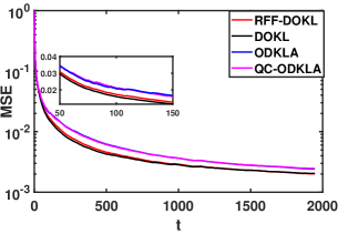
(a)

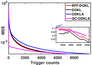
(b)

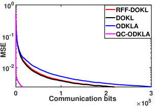
(c)

Figure 1: Learning performance on Tom’s hardware dataset. (a) MSE vs. time; (b) MSE vs. triggers; (c) MSE vs. bits.

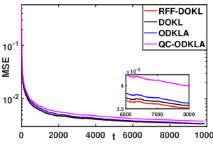
(a)

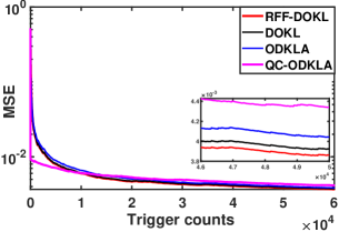
(b)

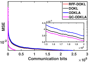
(c)

Figure 2: Learning performance on Twitter dataset. (a) MSE vs. time; (b) MSE vs. triggers; (c) MSE vs. bits.

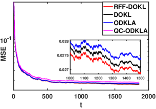
(a)

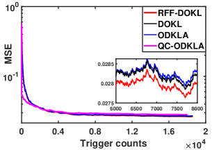
(b)

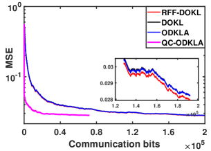
(c)

Figure 3: Learning performance on Energy dataset. (a) MSE vs. time; (b) MSE vs. triggers; (c) MSE vs. bits.

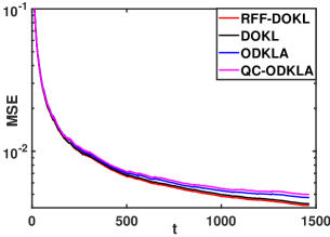
(a)

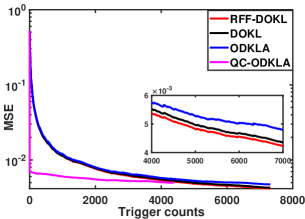
(b)

(c)

Figure 4: Learning performance on Air quality dataset. (a) MSE vs. time; (b) MSE vs. triggers; (c) MSE vs. bits.

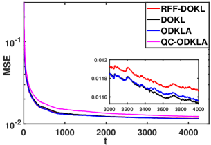
(a)

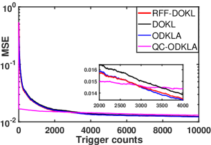
(b)

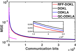
(c)

Figure 5: Learning performance on Conductivity dataset. (a) MSE vs. time; (b) MSE vs. triggers; (c) MSE vs. bits.

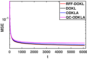
(a)

(b)

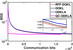
(c)

Figure 6: Learning performance on Blood dataset. (a) MSE vs. time; (b) MSE vs. triggers; (c) MSE vs. bits.

Communication efficiency. We then evaluate the communication efficiency among different algorithms. We present the MSE performance versus trigger counts in Figures 1 (b) - 6 (b) and MSE performance versus communication bits in Figures 1 (c) - 6 (c). Figures 1 (b) - 6 (b) show that QC-ODKLA triggers a few transmissions in the early learning stage, which greatly improves the communication efficiency. Further, thanks to the quantization, QC-ODKLA only needs 3 bits to transmit an element, the total number of communication bits is also greatly reduced accordingly. For other methods to transmit each element of updates, suppose the agent uses a 32-bit CPU operating mode, then the communication cost is 32 bits per iteration per agent per element. Therefore, QC-ODKLA is corroborated to greatly reduce the communication cost.

Computation efficiency. Finally, we evaluate the computation efficiency of all algorithms by their running time on six datasets, which is recorded in Table I. RFF-DOKL is a gradient descent-based first-order algorithm, which achieves the highest computation efficiency. Comparing ODKLA with the ADMM based DOKL method, we see that the linearization step reduces a large amount of computation of standard ADMM. Under the circumstance that online streaming data vary fast, a computation-efficient algorithm is preferred, reflecting the advantages of the proposed ODKLA and QC-ODKLA algorithms. Also, note that QC-ODKLA is computationally slower than ODKLA since the communication censoring and quantization steps consume computation resources.

TABLE I: The running time of four algorithms on six datasets.

Data set	RFF-DOKL	DOKL	ODKLA	QC-ODKLA
Tom’s	0.3541s	2.0613s	0.4455s	0.7247s
Twitter	4.6148s	21.8808s	6.2351s	9.4218s
Energy	0.8584s	4.2681s	1.1600s	1.7928s
Air quality	0.2760s	1.6808s	0.4717s	0.5510s
Conductivity	0.7952s	4.4285s	0.9784s	1.6201s
Blood	2.6194s	13.6249s	3.6104s	5.4290s

VII Conclusion

This paper studies the online decentralized kernel learning problem under communication constraints for multi-agent systems. We utilize RF mapping to circumvent the curse of dimensionality issue caused by the increasing size of sequentially arriving data. To efficiently solve such a challenging problem, we then develop a novel online decentralized kernel learning algorithm via linearized ADMM (ODKLA). We integrate the communication-censoring and quantization strategies into the proposed ODKAL algorithm (QC-ODKLA) to further save communication overheads. We derive the sublinear regret bound for QC-ODKLA theoretically, and verify their effectiveness in learning performance, communication and computation efficiency via simulations on various real datasets. Future work will be devoted to multi-kernel learning and dynamic kernel learning.

Appendix A Proof of Theorem V.4

Proof. Define $\bm{\Theta}^{\star}=[\bm{\theta}^{\star\top};\dots;\bm{\theta}^{\star\top}]\in\mathbb{R}^{N\times 2L}$, which is the stack of $N$ copies of $\bm{\theta}^{\star}$, and $\mathcal{L}_{t}(\bm{\Theta}^{\star}):=\sum_{i=1}^{N}\mathcal{L}_{i,t}(\bm{\theta}^{\star})$, we rewrite (23) as

$$\begin{split}\mathbf{Reg}_{T}^{S}&=\sum_{t=1}^{T}\left(\sum_{i=1}^{N}\mathcal{L}_{i,t}(\bm{\theta}_{i,t})-\sum_{i=1}^{N}\mathcal{L}_{i,t}(\bm{\theta}^{\star})\right)\\ &=\sum_{t=1}^{T}\left(\mathcal{L}_{t}(\bm{\Theta}_{t})-\mathcal{L}_{t}(\bm{\Theta}^{\star})\right).\end{split}$$ (28)

To analyze the regret bound of QC-ODKLA, we first represent the matrix form update of QC-ODKLA updates (21) - (22) as

$$\begin{split}\bm{\Theta}_{t+1}&=\bm{\Theta}_{t}-(\eta_{t}\mathbf{I}+2\rho\bm{D})^{-1}\Big{[}\partial\mathcal{L}_{t}(\bm{\Theta}_{t})\\ &\qquad\qquad\qquad\qquad\qquad+\rho(\bm{D}-\bm{W})\hat{\bm{\Theta}}_{t}+\bm{\Gamma}_{t}\Big{]},\end{split}$$ (29)

$$\begin{split}\bm{\Gamma}_{t+1}&=\bm{\Gamma}_{t}+\rho(\bm{D}-\bm{W})\hat{\bm{\Theta}}_{t+1},\end{split}$$ (30)

where $\hat{\bm{\Theta}}_{t}=[\hat{\bm{\theta}}_{1,t}^{\top};\dots;\hat{\bm{\theta}}_{N,t}^{\top}]\in\mathbb{R}^{N\times 2L}$. Note that the censoring and quantization are implemented after step (29) and before step (30).

The definitions of the introduced error in (24) and the overall introduced error $\bm{E}_{t}$ is equivalent to $\bm{E}_{t}:=\bm{\Theta}_{t}-\hat{\bm{\Theta}}_{t}$. With the equality $\mathbf{D}-\mathbf{W}=\frac{1}{2}\mathbf{S}_{-}\mathbf{S}_{-}^{\top}$, we can obtain the equivalent form of (29) and (30) respectively as

$$\begin{split}\bm{\Theta}_{t+1}&=\bm{\Theta}_{t}-(\eta_{t}\mathbf{I}+2\rho\bm{D})^{-1}\\ &\quad\Big{[}\partial\mathcal{L}_{t}(\bm{\Theta}_{t})+\frac{\rho}{2}\mathbf{S}_{-}\mathbf{S}_{-}^{\top}\bm{\Theta}_{t}-\frac{\rho}{2}\mathbf{S}_{-}\mathbf{S}_{-}^{\top}\bm{E}_{t}+\bm{\Gamma}_{t}\Big{]},\end{split}$$ (31)

$$\begin{split}\bm{\Gamma}_{t+1}&=\bm{\Gamma}_{t}+\frac{\rho}{2}\mathbf{S}_{-}\mathbf{S}_{-}^{\top}\bm{\Theta}_{t+1}-\frac{\rho}{2}\mathbf{S}_{-}\mathbf{S}_{-}^{\top}\bm{E}_{t+1}.\end{split}$$ (32)

Observe from (32) that $\bm{\Gamma}_{t+1}$ stays in the column space of $\mathbf{S}_{-}\mathbf{S}_{-}^{\top}$ if $\bm{\Gamma}_{1}$ is also initialized therein. Therefore, we introduce variables $\bm{\beta}_{t}\in\mathbb{R}^{2r\times 2L}$, which stay in the column space of $\mathbf{S}_{-}^{\top}$, and let $\bm{\Gamma}_{t}=\mathbf{S}_{-}\bm{\beta}_{t}$ for any $t\geq 1$. Then, (32) is equivalent to

$$\bm{\beta}_{t+1}=\bm{\beta}_{t}+\frac{\rho}{2}\mathbf{S}^{\top}_{-}\bm{\Theta}_{t+1}-\frac{\rho}{2}\mathbf{S}_{-}^{\top}\bm{E}_{t+1}.$$ (33)

Using (32) and $\bm{\Gamma}_{t}=\mathbf{S}_{-}\bm{\beta}_{t}$ to eliminate $\bm{\Gamma}_{t}$, we rewrite (31) as

$$\begin{split}&\bm{\Theta}_{t+1}=\bm{\Theta}_{t}-(\eta_{t}\mathbf{I}+2\rho\bm{D})^{-1}\Big{[}\partial\mathcal{L}_{t}(\bm{\Theta}_{t})+\mathbf{S}_{-}\bm{\beta}_{t+1}\\ &\quad\;\;+\frac{\rho}{2}\mathbf{S}_{-}\mathbf{S}_{-}^{\top}(\bm{E}_{t+1}-\bm{E}_{t})+\frac{\rho}{2}\mathbf{S}_{-}\mathbf{S}_{-}^{\top}(\bm{\Theta}_{t}-\bm{\Theta}_{t+1})\Big{]}.\end{split}$$ (34)

The following analysis is based on the equivalent form of the QC-ODKLA algorithm given by (34) and (33). The Karush–Kuhn–Tucker (KKT) conditions of (9) are

$$\partial\mathcal{L}_{t}(\bm{\Theta}^{\star})+\eta_{t}(\bm{\Theta}^{\star}-\bm{\Theta}_{t})+\mathbf{S}_{-}\bm{\beta}^{\star} =\mathbf{0},$$ (35a)

$$\mathbf{S}_{-}^{\top}\bm{\Theta}^{\star} =\mathbf{0},$$ (35b)

$$\frac{1}{2}\mathbf{S}_{+}^{\top}\bm{\Theta}^{\star} =\bm{Z}^{\star},$$ (35c)

where $(\bm{\Theta}^{\star},\bm{Z}^{\star},\bm{\beta}^{\star})$ is the optimal primal-dual triplet.

Rearrange terms in (34) to place $\partial\mathcal{L}_{t}(\bm{\Theta}_{t})$ at the left side, we have

$$\begin{split}\partial\mathcal{L}_{t}(\bm{\Theta}_{t})&=(\eta_{t}\mathbf{I}+2\rho\bm{D}-\frac{\rho}{2}\mathbf{S}_{-}\mathbf{S}_{-}^{\top})(\bm{\Theta}_{t}-\bm{\Theta}_{t+1})\\ &\quad+\frac{\rho}{2}\mathbf{S}_{-}\mathbf{S}_{-}^{\top}(\bm{E}_{t}-\bm{E}_{t+1})-\mathbf{S}_{-}\bm{\beta}_{t+1}\\ &=(\eta_{t}\mathbf{I}+\frac{\rho}{2}\mathbf{S}_{+}\mathbf{S}_{+}^{\top})(\bm{\Theta}_{t}-\bm{\Theta}_{t+1})\\ &\quad+\frac{\rho}{2}\mathbf{S}_{-}\mathbf{S}_{-}^{\top}(\bm{E}_{t}-\bm{E}_{t+1})-\mathbf{S}_{-}\bm{\beta}_{t+1},\end{split}$$ (36)

where the second equality utilizes $\mathbf{D}-\mathbf{W}=\frac{1}{2}\mathbf{S}_{-}\mathbf{S}_{-}^{\top}$ and $\mathbf{D}+\mathbf{W}=\frac{1}{2}\mathbf{S}_{+}\mathbf{S}_{+}^{\top}$ such that $2\mathbf{D}=\frac{1}{2}\mathbf{S}_{-}\mathbf{S}_{-}^{\top}+\frac{1}{2}\mathbf{S}_{+}\mathbf{S}_{+}^{\top}$. We consider to bound the instantaneous regret $\mathcal{L}_{t}(\bm{\Theta}_{t})-\mathcal{L}_{t}(\bm{\Theta}^{\star})$ at time $t$ first. With Assumption V.1, it holds

$$\mathcal{L}_{t}(\bm{\Theta}_{t})-\mathcal{L}_{t}(\bm{\Theta}^{\star})\leq\langle\partial\mathcal{L}_{t}(\bm{\Theta}_{t}),\bm{\Theta}_{t}-\bm{\Theta}^{\star}\rangle.$$ (37)

Substitute the expression of $\partial\mathcal{L}_{t}(\bm{\Theta}_{t})$ in (36) into (37) yields

$$\begin{split}&\quad\mathcal{L}_{t}(\bm{\Theta}_{t})-\mathcal{L}_{t}(\bm{\Theta}^{\star})\\ &\leq\langle(\eta_{t}\mathbf{I}+\frac{\rho}{2}\mathbf{S}_{+}\mathbf{S}_{+}^{\top})(\bm{\Theta}_{t}-\bm{\Theta}_{t+1}),\bm{\Theta}_{t}-\bm{\Theta}^{\star}\rangle\\ &+\langle\frac{\rho}{2}\mathbf{S}_{-}\mathbf{S}_{-}^{\top}(\bm{E}_{t}-\bm{E}_{t+1})-\mathbf{S}_{-}\bm{\beta}_{t+1},\bm{\Theta}_{t}-\bm{\Theta}^{\star}\rangle.\end{split}$$ (38)

Now we reorganize the two terms on the right-hand side of (38). For the first term, we have

$$\begin{split}&\quad\langle(\eta_{t}\mathbf{I}+\frac{\rho}{2}\mathbf{S}_{+}\mathbf{S}_{+}^{\top})(\bm{\Theta}_{t}-\bm{\Theta}_{t+1}),\bm{\Theta}_{t}-\bm{\Theta}^{\star}\rangle\\ &\leq\sigma_{\max}(\eta_{t}\mathbf{I}+\frac{\rho}{2}\mathbf{S}_{+}\mathbf{S}_{+}^{\top})\langle\bm{\Theta}_{t}-\bm{\Theta}_{t+1},\bm{\Theta}_{t}-\bm{\Theta}^{\star}\rangle\\ &=\frac{\sigma_{\max}(\eta_{t}\mathbf{I}+\frac{\rho}{2}\mathbf{S}_{+}\mathbf{S}_{+}^{\top})}{2}\Big{(}\|\bm{\Theta}_{t}-\bm{\Theta}^{\star}\|_{F}^{2}\\ &\quad-\|\bm{\Theta}_{t+1}-\bm{\Theta}^{\star}\|_{F}^{2}+\|\bm{\Theta}_{t}-\bm{\Theta}_{t+1}\|_{F}^{2}\Big{)},\end{split}$$ (39)

where $\sigma_{\max}(\eta_{t}\mathbf{I}+\frac{\rho}{2}\mathbf{S}_{+}\mathbf{S}_{+}^{\top})$ denotes the maximum singular value of $\eta_{t}\mathbf{I}+\frac{\rho}{2}\mathbf{S}_{+}\mathbf{S}_{+}^{\top}$.

For the second term, we have

$$\begin{split}&\langle\frac{\rho}{2}\mathbf{S}_{-}\mathbf{S}_{-}^{\top}(\bm{E}_{t}-\bm{E}_{t+1})-\mathbf{S}_{-}\bm{\beta}_{t+1},\bm{\Theta}_{t}-\bm{\Theta}^{\star}\rangle\\ &=\langle\frac{\rho}{2}\mathbf{S}_{-}^{\top}(\bm{E}_{t}-\bm{E}_{t+1})-\bm{\beta}_{t+1},\mathbf{S}_{-}^{\top}(\bm{\Theta}_{t}-\bm{\Theta}^{\star})\rangle\\ &\stackrel{{\scriptstyle(a)}}{{=}}\langle\frac{\rho}{2}\mathbf{S}_{-}^{\top}(\bm{E}_{t}-\bm{E}_{t+1})-\bm{\beta}_{t+1},\mathbf{S}_{-}^{\top}\bm{\Theta}_{t}\rangle\\ &\stackrel{{\scriptstyle(b)}}{{=}}\langle\frac{\rho}{2}\mathbf{S}_{-}^{\top}(\bm{E}_{t}-\bm{E}_{t+1})-\bm{\beta}_{t+1},\frac{2}{\rho}(\bm{\beta}_{t}-\bm{\beta}_{t-1})+\mathbf{S}_{-}^{\top}\bm{E}_{t}\rangle\\ &=\langle\bm{\beta}_{t-1}-2\bm{\beta}_{t}+\frac{\rho}{2}\mathbf{S}_{-}^{\top}(\bm{\Theta}_{t}-\bm{\Theta}_{t+1}),\frac{2}{\rho}(\bm{\beta}_{t}-\bm{\beta}_{t-1})+\mathbf{S}_{-}^{\top}\bm{E}_{t}\rangle\\ &\stackrel{{\scriptstyle(c)}}{{=}}-\frac{2}{\rho}\langle\bm{\beta}_{t}-\bm{\beta}_{t-1},\bm{\beta}_{t}-\bm{\beta}_{t-1}\rangle-\frac{2}{\rho}\langle\bm{\beta}_{t},\bm{\beta}_{t}-\bm{\beta}_{t-1}\rangle\\ &\quad+\langle\bm{\beta}_{t-1}-\bm{\beta}_{t},\mathbf{S}_{-}^{\top}\bm{E}_{t}\rangle+\langle\mathbf{S}_{-}^{\top}(\bm{\Theta}_{t}-\bm{\Theta}_{t+1}),\bm{\beta}_{t}-\bm{\beta}_{t-1}\rangle\\ &\quad+\frac{\rho}{2}\langle\mathbf{S}_{-}^{\top}(\bm{\Theta}_{t}-\bm{\Theta}_{t+1}),\mathbf{S}_{-}^{\top}\bm{E}_{t}\rangle-\langle\bm{\beta}_{t},\mathbf{S}_{-}^{\top}\bm{E}_{t}\rangle\\ &=-\frac{2}{\rho}\|\bm{\beta}_{t}-\bm{\beta}_{t-1}\|_{F}^{2}-\frac{2}{\rho}\|\bm{\beta}_{t}\|_{F}^{2}+\frac{2}{\rho}\langle\bm{\beta}_{t},\bm{\beta}_{t-1}\rangle-\langle\bm{\beta}_{t},\mathbf{S}_{-}^{\top}\bm{E}_{t}\rangle\\ &\quad+\langle\bm{\beta}_{t-1}-\bm{\beta}_{t},\mathbf{S}_{-}^{\top}\bm{E}_{t}\rangle+\langle\mathbf{S}_{-}^{\top}(\bm{\Theta}_{t}-\bm{\Theta}_{t+1}),\bm{\beta}_{t}-\bm{\beta}_{t-1}\rangle\\ &\quad+\frac{\rho}{2}\langle\mathbf{S}_{-}^{\top}(\bm{\Theta}_{t}-\bm{\Theta}_{t+1}),\mathbf{S}_{-}^{\top}\bm{E}_{t}\rangle,\\ \end{split}$$ (40)

where (a) comes from the KKT condition (35b), (b) and (c) are obtained by utilizing (33).

Next, we will utilize Young’s inequality to bound the inner product terms in (40), which are

$$\begin{split}&\frac{2}{\rho}\langle\bm{\beta}_{t},\bm{\beta}_{t-1}\rangle\leq\frac{2}{\rho}(\frac{1}{2\eta_{1}}\|\bm{\beta}_{t}\|_{F}^{2}+\frac{\eta_{1}}{2}\|\bm{\beta}_{t-1}\|_{F}^{2})\\ &\qquad\qquad\quad=\frac{1}{\rho\eta_{1}}\|\bm{\beta}_{t}\|_{F}^{2}+\frac{\eta_{1}}{\rho}\|\bm{\beta}_{t-1}\|_{F}^{2},\\ &\langle\bm{\beta}_{t-1}-\bm{\beta}_{t},\mathbf{S}_{-}^{\top}\bm{E}_{t}\rangle\leq\frac{1}{2\eta_{2}}\|\bm{\beta}_{t-1}-\bm{\beta}_{t}\|_{F}^{2}+\frac{\eta_{2}}{2}\|\mathbf{S}_{-}^{\top}\bm{E}_{t}\|_{F}^{2},\\ &-\langle\bm{\beta}_{t},\mathbf{S}_{-}^{\top}\bm{E}_{t}\rangle\leq\frac{1}{2\eta_{3}}\|\bm{\beta}_{t}\|_{F}^{2}+\frac{\eta_{3}}{2}\|\mathbf{S}_{-}^{\top}\bm{E}_{t}\|_{F}^{2},\\ &\langle\mathbf{S}_{-}^{\top}(\bm{\Theta}_{t}-\bm{\Theta}_{t+1}),\bm{\beta}_{t}-\bm{\beta}_{t-1}\rangle\leq\frac{1}{2\eta_{4}}\|\mathbf{S}_{-}^{\top}(\bm{\Theta}_{t}-\bm{\Theta}_{t+1})\|_{F}^{2}\\ &\qquad\qquad\quad\qquad\qquad\quad\qquad\quad+\frac{\eta_{4}}{2}\|\bm{\beta}_{t}-\bm{\beta}_{t-1}\|_{F}^{2},\\ &\frac{\rho}{2}\langle\mathbf{S}_{-}^{\top}(\bm{\Theta}_{t}-\bm{\Theta}_{t+1}),\mathbf{S}_{-}^{\top}\bm{E}_{t}\rangle\leq\frac{\rho}{4\eta_{5}}\|\mathbf{S}_{-}^{\top}(\bm{\Theta}_{t}-\bm{\Theta}_{t+1})\|_{F}^{2}\\ &\qquad\qquad\qquad\qquad\qquad\qquad+\frac{\rho\eta_{5}}{4}\|\mathbf{S}_{-}^{\top}\bm{E}_{t}\|_{F}^{2},\end{split}$$ (41)

where $\eta_{1},\eta_{2},\eta_{3},\eta_{4},\eta_{5}$ are any positive constants.

Substitute (41) into (40) gives

$$\begin{split}&\langle\frac{\rho}{2}\mathbf{S}_{-}\mathbf{S}_{-}^{\top}(\bm{E}_{t}-\bm{E}_{t+1})-\mathbf{S}_{-}\bm{\beta}_{t+1},\bm{\Theta}_{t}-\bm{\Theta}^{\star}\rangle\\ &\leq(-\frac{2}{\rho}+\frac{1}{2\eta_{2}}+\frac{\eta_{4}}{2})\|\bm{\beta}_{t}-\bm{\beta}_{t-1}\|_{F}^{2}+\frac{\eta_{1}}{\rho}\|\bm{\beta}_{t-1}\|_{F}^{2}\\ &\quad+(-\frac{2}{\rho}+\frac{1}{\rho\eta_{1}}+\frac{1}{2\eta_{3}})\|\bm{\beta}_{t}\|_{F}^{2}\\ &\quad+(\frac{1}{2\eta_{4}}+\frac{\rho}{4\eta_{5}})\|\mathbf{S}_{-}^{\top}(\bm{\Theta}_{t}-\bm{\Theta}_{t+1})\|_{F}^{2}\\ &\quad+(\frac{\eta_{2}}{2}+\frac{\eta_{3}}{2}+\frac{\rho\eta_{5}}{4})\|\mathbf{S}_{-}^{\top}\bm{E}_{t}\|_{F}^{2}\\ &=(-\frac{2}{\rho}+\frac{1}{2\eta_{2}}+\frac{\eta_{4}}{2})(\|\bm{\beta}_{t}\|_{F}^{2}+\|\bm{\beta}_{t-1}\|_{F}^{2}-2\langle\bm{\beta}_{t},\bm{\beta}_{t-1}\rangle)\\ &\quad+(-\frac{2}{\rho}+\frac{1}{\rho\eta_{1}}+\frac{1}{2\eta_{3}})\|\bm{\beta}_{t}\|_{F}^{2}+\frac{\eta_{1}}{\rho}\|\bm{\beta}_{t-1}\|_{F}^{2}\\ &\quad+(\frac{1}{2\eta_{4}}+\frac{\rho}{4\eta_{5}})\|\mathbf{S}_{-}^{\top}(\bm{\Theta}_{t}-\bm{\Theta}_{t+1})\|_{F}^{2}\\ &\quad+(\frac{\eta_{2}}{2}+\frac{\eta_{3}}{2}+\frac{\rho\eta_{5}}{4})\|\mathbf{S}_{-}^{\top}\bm{E}_{t}\|_{F}^{2}\\ &=(-\frac{4}{\rho}+\frac{1}{2\eta_{2}}+\frac{\eta_{4}}{2}+\frac{1}{\rho\eta_{1}}+\frac{1}{2\eta_{3}})\|\bm{\beta}_{t}\|_{F}^{2}\\ &\quad+(-\frac{2}{\rho}+\frac{1}{2\eta_{2}}+\frac{\eta_{4}}{2}+\frac{\eta_{1}}{\rho})\|\bm{\beta}_{t-1}\|_{F}^{2}\\ &\quad+(\frac{1}{2\eta_{4}}+\frac{\rho}{4\eta_{5}})\|\mathbf{S}_{-}^{\top}(\bm{\Theta}_{t}-\bm{\Theta}_{t+1})\|_{F}^{2}\\ &\quad+(\frac{\eta_{2}}{2}+\frac{\eta_{3}}{2}+\frac{\rho\eta_{5}}{4})\|\mathbf{S}_{-}^{\top}\bm{E}_{t}\|_{F}^{2}\\ &\quad+(\frac{2}{\rho}-\frac{1}{2\eta_{2}}-\frac{\eta_{4}}{2})\langle\bm{\beta}_{t},\bm{\beta}_{t-1}\rangle\\ &\leq\Big{(}-\frac{4}{\rho}+\frac{1}{2\eta_{2}}+\frac{\eta_{4}}{2}+\frac{1}{\rho\eta_{1}}+\frac{1}{2\eta_{3}}+\frac{2}{\rho\eta_{6}}\\ &\qquad-\frac{1}{2\eta_{2}\eta_{6}}-\frac{\eta_{4}}{2\eta_{6}}\Big{)}\|\bm{\beta}_{t}\|_{F}^{2}\\ &\quad+\Big{(}-\frac{2}{\rho}+\frac{1}{2\eta_{2}}+\frac{\eta_{4}}{2}+\frac{\eta_{1}}{\rho}+\frac{2\eta_{6}}{\rho}\\ &\qquad-\frac{\eta_{6}}{2\eta_{2}}-\frac{\eta_{4}\eta_{6}}{2}\Big{)}\|\bm{\beta}_{t-1}\|_{F}^{2}\\ &\quad+\Big{(}\frac{1}{2\eta_{4}}+\frac{\rho}{4\eta_{5}}\Big{)}\|\mathbf{S}_{-}^{\top}(\bm{\Theta}_{t}-\bm{\Theta}_{t+1})\|_{F}^{2}\\ &\quad+\Big{(}\frac{\eta_{2}}{2}+\frac{\eta_{3}}{2}+\frac{\rho\eta_{5}}{4}\Big{)}\|\mathbf{S}_{-}^{\top}\bm{E}_{t}\|_{F}^{2}.\\ \end{split}$$ (42)

With (42) and (39), we obtain an upper bound for (38), which is

$$\begin{split}&\mathcal{L}_{t}(\bm{\Theta}_{t})-\mathcal{L}_{t}(\bm{\Theta}^{\star})\\ &\leq\frac{\sigma_{\max}(\eta_{t}\mathbf{I}+\frac{\rho}{2}\mathbf{S}_{+}\mathbf{S}_{+}^{\top})}{2}\Big{(}\|\bm{\Theta}_{t}-\bm{\Theta}^{\star}\|_{F}^{2}-\|\bm{\Theta}_{t+1}-\bm{\Theta}^{\star}\|_{F}^{2}\Big{)}\\ &\quad+\frac{\sigma_{\max}(\eta_{t}\mathbf{I}+\frac{\rho}{2}\mathbf{S}_{+}\mathbf{S}_{+}^{\top})}{2}\|\bm{\Theta}_{t}-\bm{\Theta}_{t+1}\|_{F}^{2}\\ &\quad+(\frac{1}{2\eta_{2}}-\frac{4}{\rho}+\frac{\eta_{4}}{2}+\frac{1}{\rho\eta_{1}}+\frac{1}{2\eta_{3}}+\frac{2}{\rho\eta_{6}}-\frac{1}{2\eta_{2}\eta_{6}}-\frac{\eta_{4}}{2\eta_{6}})\|\bm{\beta}_{t}\|_{F}^{2}\\ &\quad+(\frac{\eta_{1}}{\rho}-\frac{2}{\rho}+\frac{1}{2\eta_{2}}+\frac{\eta_{4}}{2}+\frac{2\eta_{6}}{\rho}-\frac{\eta_{6}}{2\eta_{2}}-\frac{\eta_{4}\eta_{6}}{2})\|\bm{\beta}_{t-1}\|_{F}^{2}\\ &\quad+(\frac{1}{2\eta_{4}}+\frac{\rho}{4\eta_{5}})\|\mathbf{S}_{-}^{\top}(\bm{\Theta}_{t}-\bm{\Theta}_{t+1})\|_{F}^{2}+(\frac{\eta_{2}}{2}+\frac{\eta_{3}}{2}+\frac{\rho\eta_{5}}{4})\|\mathbf{S}_{-}^{\top}\bm{E}_{t}\|_{F}^{2}\\ &\leq\frac{\sigma_{\max}(\eta_{t}\mathbf{I}+\frac{\rho}{2}\mathbf{S}_{+}\mathbf{S}_{+}^{\top})}{2}\Big{(}\|\bm{\Theta}_{t}-\bm{\Theta}^{\star}\|_{F}^{2}-\|\bm{\Theta}_{t+1}-\bm{\Theta}^{\star}\|_{F}^{2}\Big{)}\\ &\quad+(\frac{1}{2\eta_{2}}-\frac{4}{\rho}+\frac{\eta_{4}}{2}+\frac{1}{\rho\eta_{1}}+\frac{1}{2\eta_{3}}+\frac{2}{\rho\eta_{6}}-\frac{1}{2\eta_{2}\eta_{6}}-\frac{\eta_{4}}{2\eta_{6}})\|\bm{\beta}_{t}\|_{F}^{2}\\ &\quad+(\frac{\eta_{1}}{\rho}-\frac{2}{\rho}+\frac{1}{2\eta_{2}}+\frac{\eta_{4}}{2}+\frac{2\eta_{6}}{\rho}-\frac{\eta_{6}}{2\eta_{2}}-\frac{\eta_{4}\eta_{6}}{2})\|\bm{\beta}_{t-1}\|_{F}^{2}\\ &\quad+(\frac{\sigma_{\max}(\eta_{t}\mathbf{I}+\frac{\rho}{2}\mathbf{S}_{+}\mathbf{S}_{+}^{\top})}{2}+\frac{\sigma^{2}_{\max}(\mathbf{S}_{-})}{2\eta_{4}}+\frac{\rho\sigma^{2}_{\max}(\mathbf{S}_{-})}{4\eta_{5}})\|\bm{\Theta}_{t}-\bm{\Theta}_{t+1}\|_{F}^{2}\\ &\quad+(\frac{\eta_{2}}{2}+\frac{\eta_{3}}{2}+\frac{\rho\eta_{5}}{4})\sigma^{2}_{\max}(\mathbf{S}_{-})\|\bm{E}_{t}\|_{F}^{2}.\end{split}$$ (43)

We then utilize (34) to rewrite $\bm{\Theta}_{t}-\bm{\Theta}_{t+1}$ as

$$\bm{\Theta}_{t}-\bm{\Theta}_{t+1}=(\eta_{t}\mathbf{I}+2\rho\bm{D})^{-1}\Big{(}\partial\mathcal{L}_{t}(\bm{\Theta}_{t})+2\mathbf{S}_{-}\bm{\beta}_{t}-\mathbf{S}_{-}\bm{\beta}_{t-1}\Big{)},$$ (44)

and bound $\|\bm{\Theta}_{t}-\bm{\Theta}_{t+1}\|_{F}^{2}$ as

$$\begin{split}\|\bm{\Theta}_{t}-\bm{\Theta}_{t+1}\|_{F}^{2}&=\|(\eta_{t}\mathbf{I}+2\rho\bm{D})^{-1}\Big{(}\partial\mathcal{L}_{t}(\bm{\Theta}_{t})+2\mathbf{S}_{-}\bm{\beta}_{t}-\mathbf{S}_{-}\bm{\beta}_{t-1}\Big{)}\|_{F}^{2}\\ &\leq\frac{1}{\sigma^{2}_{\min}(\eta_{t}\mathbf{I}+2\rho\bm{D})}\|\partial\mathcal{L}_{t}(\bm{\Theta}_{t})\|_{F}^{2}\\ &+\frac{4\sigma^{2}_{\max}(\mathbf{S}_{-})}{\sigma^{2}_{\min}(\eta_{t}\mathbf{I}+2\rho\bm{D})}\|\bm{\beta}_{t}\|_{F}^{2}\\ &+\frac{\sigma^{2}_{\max}(\mathbf{S}_{-})}{\sigma^{2}_{\min}(\eta_{t}\mathbf{I}+2\rho\bm{D})}\|\bm{\beta}_{t-1}\|_{F}^{2},\end{split}$$ (45)

where $\sigma_{\min}(\eta_{t}\mathbf{I}+2\rho\bm{D})$ is the lower bound of the nonzero singular values of $\eta_{t}\mathbf{I}+2\rho\bm{D}$.

Substitute (45) into (43) we obtain

$$\begin{split}\mathcal{L}_{t}(\bm{\Theta}_{t})-\mathcal{L}_{t}(\bm{\Theta}^{\star})&\leq\frac{\sigma_{\max}(\eta_{t}\mathbf{I}+\frac{\rho}{2}\mathbf{S}_{+}\mathbf{S}_{+}^{\top})}{2}\Big{(}\|\bm{\Theta}_{t}-\bm{\Theta}^{\star}\|_{F}^{2}\\ &-\|\bm{\Theta}_{t+1}-\bm{\Theta}^{\star}\|_{F}^{2}\Big{)}+(c_{1}+4c_{\mathcal{N}})\|\bm{\beta}_{t}\|_{F}^{2}\\ &+(c_{2}+c_{\mathcal{N}})\|\bm{\beta}_{t-1}\|_{F}^{2}+\frac{c_{\mathcal{N}}}{\sigma^{2}_{\max}(\mathbf{S}_{-})}\|\partial\mathcal{L}_{t}(\bm{\Theta}_{t})\|_{F}^{2}\\ &+(\frac{\eta_{2}}{2}+\frac{\eta_{3}}{2}+\frac{\rho\eta_{5}}{4})\sigma^{2}_{\max}(\mathbf{S}_{-})\|\bm{E}_{t}\|_{F}^{2},\end{split}$$ (46)

where $c_{1},c_{2}$ and $c_{\mathcal{N}}$ are defined as follows:

$$\begin{split}c_{1}&:=\frac{1}{2\eta_{2}}-\frac{4}{\rho}+\frac{\eta_{4}}{2}+\frac{1}{\rho\eta_{1}}+\frac{1}{2\eta_{3}}+\frac{2}{\rho\eta_{6}}-\frac{1}{2\eta_{2}\eta_{6}}-\frac{\eta_{4}}{2\eta_{6}},\\ c_{2}&:=\frac{\eta_{1}}{\rho}-\frac{2}{\rho}+\frac{1}{2\eta_{2}}+\frac{\eta_{4}}{2}+\frac{2\eta_{6}}{\rho}-\frac{\eta_{6}}{2\eta_{2}}-\frac{\eta_{4}\eta_{6}}{2},\\ c_{\mathcal{N}}&:=\Big{(}\frac{\sigma_{\max}(\eta_{t}\mathbf{I}+\frac{\rho}{2}\mathbf{S}_{+}\mathbf{S}_{+}^{\top})}{2}+\frac{\sigma^{2}_{\max}(\mathbf{S}_{-})}{2\eta_{4}}+\frac{\rho\sigma^{2}_{\max}(\mathbf{S}_{-})}{4\eta_{5}}\Big{)}\\ &\qquad\frac{\sigma^{2}_{\max}(\mathbf{S}_{-})}{\sigma^{2}_{\min}(\eta_{t}\mathbf{I}+2\rho\bm{D})}.\end{split}$$

Carefully choose $\eta_{1},\eta_{2},\eta_{3},\eta_{4},\eta_{5}$, and $\eta_{6}$, we can make $c_{1}+4c_{\mathcal{N}}=-(c_{2}+c_{\mathcal{N}})=-c$, where $c>0$. Then (46) can be further simplified as

$$\begin{split}&\mathcal{L}_{t}(\bm{\Theta}_{t})-\mathcal{L}_{t}(\bm{\Theta}^{\star})\\ &\leq\frac{\sigma_{\max}(\eta_{t}\mathbf{I}+\frac{\rho}{2}\mathbf{S}_{+}\mathbf{S}_{+}^{\top})}{2}\Big{(}\|\bm{\Theta}_{t}-\bm{\Theta}^{\star}\|_{F}^{2}-\|\bm{\Theta}_{t+1}-\bm{\Theta}^{\star}\|_{F}^{2}\Big{)}\\ &+c(\|\bm{\beta}_{t-1}\|_{F}^{2}-\|\bm{\beta}_{t}\|_{F}^{2})+\frac{c_{\mathcal{N}}}{\sigma^{2}_{\max}(\mathbf{S}_{-})}\|\partial\mathcal{L}_{t}(\bm{\Theta}_{t})\|_{F}^{2}\\ &+(\frac{\eta_{2}}{2}+\frac{\eta_{3}}{2}+\frac{\rho\eta_{5}}{4})\sigma^{2}_{\max}(\mathbf{S}_{-})\|\bm{E}_{t}\|_{F}^{2}.\end{split}$$ (47)

To satisfy $c_{1}+4c_{\mathcal{N}}=-(c_{2}+c_{\mathcal{N}})$, one example is to set $\eta_{4}=\frac{2\eta_{6}}{(\eta_{6}-1)^{2}}(\frac{1}{\rho}(\eta_{1}+\frac{1}{\eta_{1}}+\frac{2}{\eta_{6}}+2\eta_{6})+\frac{1}{2\eta_{2}}(2-\eta_{6}-\frac{1}{\eta_{6}})+\frac{1}{2\eta_{3}}+5c_{\mathcal{N}})$.

Summarizing both sides of (47) from $t=1$ to $t=T$ leads to the accumulated network regret $\mathcal{R}(T)$:

$$\begin{split}&\quad\mathcal{R}(T)\\ &\leq\frac{\sigma_{\max}(\eta_{t}\mathbf{I}+\frac{\rho}{2}\mathbf{S}_{+}\mathbf{S}_{+}^{\top})}{2}\Big{(}\|\bm{\Theta}_{1}-\bm{\Theta}^{\star}\|_{F}^{2}-\|\bm{\Theta}_{T+1}-\bm{\Theta}^{\star}\|_{F}^{2}\Big{)}\\ &+c(\|\bm{\beta}_{0}\|_{F}^{2}-\|\bm{\beta}_{T}\|_{F}^{2})+\sum_{t=1}^{T}\frac{c_{\mathcal{N}}}{\sigma^{2}_{\max}(\mathbf{S}_{-})}\|\partial\mathcal{L}_{t}(\bm{\Theta}_{t})\|_{F}^{2}\\ &+\sum_{t=1}^{T}(\frac{\eta_{2}}{2}+\frac{\eta_{3}}{2}+\frac{\rho\eta_{5}}{4})\sigma^{2}_{\max}(\mathbf{S}_{-})\|\bm{E}_{t}\|_{F}^{2}\\ &\leq\frac{\sigma_{\max}(\eta_{t}\mathbf{I}+\frac{\rho}{2}\mathbf{S}_{+}\mathbf{S}_{+}^{\top})}{2}\|\bm{\Theta}_{1}-\bm{\Theta}^{\star}\|_{F}^{2}+c\|\bm{\beta}_{0}\|_{F}^{2}\\ &+\sum_{t=1}^{T}\frac{c_{\mathcal{N}}}{\sigma^{2}_{\max}(\mathbf{S}_{-})}\|\partial\mathcal{L}_{t}(\bm{\Theta}_{t})\|_{F}^{2}\\ &+\sum_{t=1}^{T}(\frac{\eta_{2}}{2}+\frac{\eta_{3}}{2}+\frac{\rho\eta_{5}}{4})\sigma^{2}_{\max}(\mathbf{S}_{-})\|\bm{E}_{t}\|_{F}^{2}\\ &=\frac{\sigma_{\max}(\eta_{t}\mathbf{I}+\frac{\rho}{2}\mathbf{S}_{+}\mathbf{S}_{+}^{\top})}{2}\|\bm{\Theta}^{\star}\|_{F}^{2}\\ &+\sum_{t=1}^{T}\frac{c_{\mathcal{N}}}{\sigma^{2}_{\max}(\mathbf{S}_{-})}\|\partial\mathcal{L}_{t}(\bm{\Theta}_{t})\|_{F}^{2}\\ &+\sum_{t=1}^{T}(\frac{\eta_{2}}{2}+\frac{\eta_{3}}{2}+\frac{\rho\eta_{5}}{4})\sigma^{2}_{\max}(\mathbf{S}_{-})\|\bm{E}_{t}\|_{F}^{2}.\end{split}$$ (48)

The last equality comes from the initialization that $\bm{\Theta}_{1}=\mathbf{0}$ and $\bm{\beta}_{1}=\mathbf{0}$ and thus $\bm{\beta}_{0}=\mathbf{0}$. Assumption V.2 assumes $\|\bm{\theta}^{\star}\|_{F}\leq C_{\theta}$, which implies $\|\bm{\Theta}^{\star}\|_{F}\leq\sqrt{N}C_{\theta}$. Assumption V.1 assumes $\|\partial\mathcal{L}_{t}(\bm{\Theta}_{t})\|_{F}\leq C_{\mathcal{L}}$. Then, setting $\rho=\eta_{t}=\eta_{2}=\eta_{3}=1/\mathcal{O}(\sqrt{T})$, the sublinear regret is achieved:

$$\mathcal{R}(T)\leq(\sqrt{N}C_{\theta}+\frac{1}{\sigma^{2}_{\max}(\mathbf{S}_{-})}C_{\mathcal{L}}+\sigma^{2}_{\max}(\mathbf{S}_{-})\zeta)\mathcal{O}(\sqrt{T}),$$ (49)

where $\zeta:=\max\{\sqrt{N}\alpha\beta,\sqrt{2NL}\Delta/2\}$ with $\alpha$ and $\beta$ being the predefined censoring threshold parameters and $\Delta$ being the length of the quantization interval.

Appendix B References Section

References

• [1] Jinling Liang, Zidong Wang, Bo Shen, and Xiaohui Liu, “Distributed state estimation in sensor networks with randomly occurring nonlinearities subject to time delays,” ACM Transactions on Sensor Networks (TOSN), vol. 9, no. 1, pp. 1–18, 2012.
• [2] Wei Ren, Randal W Beard, and Ella M Atkins, “Information consensus in multivehicle cooperative control,” IEEE Control Systems Magazine, vol. 27, no. 2, pp. 71–82, 2007.
• [3] David Mateos-Núnez and Jorge Cortés, “Distributed online convex optimization over jointly connected digraphs,” IEEE Transactions on Network Science and Engineering, vol. 1, no. 1, pp. 23–37, 2014.
• [4] Hao-Feng Xu, Qing Ling, and Alejandro Ribeiro, “Online learning over a decentralized network through ADMM,” Journal of the Operations Research Society of China, vol. 3, no. 4, pp. 537–562, 2015.
• [5] Alec Koppel, Felicia Y Jakubiec, and Alejandro Ribeiro, “A saddle point algorithm for networked online convex optimization,” IEEE Transactions on Signal Processing, vol. 63, no. 19, pp. 5149–5164, 2015.
• [6] Yawei Zhao, Chen Yu, Peilin Zhao, Hanlin Tang, Shuang Qiu, and Ji Liu, “Decentralized online learning: Take benefits from others’ data without sharing your own to track global trend,” arXiv preprint arXiv:1901.10593, 2019.
• [7] Pranay Sharma, Prashant Khanduri, Lixin Shen, Donald J Bucci Jr, and Pramod K Varshney, “On distributed online convex optimization with sublinear dynamic regret and fit,” arXiv preprint arXiv:2001.03166, 2020.
• [8] Martin Zinkevich, “Online convex programming and generalized infinitesimal gradient ascent,” in International Conference on Machine Learning (ICML). PMLR, 2003, pp. 928–936.
• [9] Elad Hazan, Amit Agarwal, and Satyen Kale, “Logarithmic regret algorithms for online convex optimization,” Machine Learning, vol. 69, no. 2, pp. 169–192, 2007.
• [10] Michael Kamp, Mario Boley, Daniel Keren, Assaf Schuster, and Izchak Sharfman, “Communication-efficient distributed online prediction by dynamic model synchronization,” in Joint European Conference on Machine Learning and Knowledge Discovery in Databases. Springer, 2014, pp. 623–639.
• [11] Shahin Shahrampour and Ali Jadbabaie, “Distributed online optimization in dynamic environments using mirror descent,” IEEE Transactions on Automatic Control, vol. 63, no. 3, pp. 714–725, 2017.
• [12] Seyed Mohammad Asghari, Yi Ouyang, and Ashutosh Nayyar, “Regret bounds for decentralized learning in cooperative multi-agent dynamical systems,” in Conference on Uncertainty in Artificial Intelligence. PMLR, 2020, pp. 121–130.
• [13] Rishabh Dixit, Amrit Singh Bedi, and Ketan Rajawat, “Online learning over dynamic graphs via distributed proximal gradient algorithm,” IEEE Transactions on Automatic Control, vol. 66, no. 11, pp. 5065–5079, 2020.
• [14] Yawei Zhao, Shuang Qiu, Kuan Li, Lailong Luo, Jianping Yin, and Ji Liu, “Proximal online gradient is optimum for dynamic regret: A general lower bound,” IEEE Transactions on Neural Networks and Learning Systems, 2021.
• [15] Ping Xu, Yue Wang, Xiang Chen, and Zhi Tian, “COKE: Communication-censored decentralized kernel learning,” Journal of Machine Learning Research, vol. 22, no. 196, pp. 1–35, 2021.
• [16] Bin Gu, Miao Xin, Zhouyuan Huo, and Heng Huang, “Asynchronous doubly stochastic sparse kernel learning,” in Thirty-Second AAAI Conference on Artificial Intelligence, 2018.
• [17] Trung Le, Vu Nguyen, Tu Dinh Nguyen, and Dinh Phung, “Nonparametric budgeted stochastic gradient descent,” in Artificial Intelligence and Statistics, 2016, pp. 654–572.
• [18] Alec Koppel, Garrett Warnell, Ethan Stump, and Alejandro Ribeiro, “Parsimonious online learning with kernels via sparse projections in function space,” in 2017 IEEE International Conference on Acoustics, Speech and Signal Processing (ICASSP). IEEE, 2017, pp. 4671–4675.
• [19] Cédric Richard, José Carlos M Bermudez, and Paul Honeine, “Online prediction of time series data with kernels,” IEEE Transactions on Signal Processing, vol. 57, no. 3, pp. 1058–1067, 2008.
• [20] Bo Dai, Bo Xie, Niao He, Yingyu Liang, Anant Raj, Maria-Florina F Balcan, and Le Song, “Scalable kernel methods via doubly stochastic gradients,” in Advances in Neural Information Processing Systems, 2014, pp. 3041–3049.
• [21] Ali Rahimi and Benjamin Recht, “Random features for large-scale kernel machines,” in Advances in Neural Information Processing Systems, 2008, pp. 1177–1184.
• [22] Tu Dinh Nguyen, Trung Le, Hung Bui, and Dinh Phung, “Large-scale online kernel learning with random feature reparameterization,” in Proceedings of the 26th International Joint Conference on Artificial Intelligence (IJCAI). AAAI Press, 2017, pp. 2543–2549.
• [23] Dominic Richards, Patrick Rebeschini, and Lorenzo Rosasco, “Decentralised learning with random features and distributed gradient descent,” in International Conference on Machine Learning. PMLR, 2020, pp. 8105–8115.
• [24] Pantelis Bouboulis, Symeon Chouvardas, and Sergios Theodoridis, “Online distributed learning over networks in RKH spaces using random fourier features,” IEEE Transactions on Signal Processing, vol. 66, no. 7, pp. 1920–1932, 2018.
• [25] Yanning Shen, Saeed Karimi-Bidhendi, and Hamid Jafarkhani, “Distributed and quantized online multi-kernel learning,” IEEE Transactions on Signal Processing, vol. 69, pp. 5496–5511, 2021.
• [26] Songnam Hong and Jeongmin Chae, “Distributed online learning with multiple kernels,” IEEE Transactions on Neural Networks and Learning Systems, 2021.
• [27] Guannan Qu and Na Li, “Harnessing smoothness to accelerate distributed optimization,” IEEE Transactions on Control of Network Systems, vol. 5, no. 3, pp. 1245–1260, 2017.
• [28] Guannan Qu and Na Li, “Accelerated distributed nesterov gradient descent,” IEEE Transactions on Automatic Control, vol. 65, no. 6, pp. 2566–2581, 2019.
• [29] Shengyu Zhu, Mingyi Hong, and Biao Chen, “Quantized consensus ADMM for multi-agent distributed optimization,” in 2016 IEEE International Conference on Acoustics, Speech and Signal Processing (ICASSP). IEEE, 2016, pp. 4134–4138.
• [30] Mingrui Zhang, Lin Chen, Aryan Mokhtari, Hamed Hassani, and Amin Karbasi, “Quantized frank-wolfe: Communication-efficient distributed optimization,” arXiv preprint arXiv:1902.06332, 2019.
• [31] Sebastian U Stich, Jean-Baptiste Cordonnier, and Martin Jaggi, “Sparsified SGD with memory,” in Advances in Neural Information Processing Systems, pp. 4447–4458. 2018.
• [32] Ibrahim El Khalil Harrane, Rémi Flamary, and Cédric Richard, “On reducing the communication cost of the diffusion LMS algorithm,” IEEE Transactions on Signal and Information Processing over Networks, vol. 5, no. 1, pp. 100–112, 2018.
• [33] Mu Li, David G Andersen, Alexander J Smola, and Kai Yu, “Communication efficient distributed machine learning with the parameter server,” in Advances in Neural Information Processing Systems, 2014, pp. 19–27.
• [34] Reza Arablouei, Stefan Werner, Kutluyıl Doğançay, and Yih-Fang Huang, “Analysis of a reduced-communication diffusion LMS algorithm,” Signal Processing, vol. 117, pp. 355–361, 2015.
• [35] H Brendan McMahan, Eider Moore, Daniel Ramage, Seth Hampson, et al., “Communication-efficient learning of deep networks from decentralized data,” arXiv preprint arXiv:1602.05629, 2016.
• [36] Wotao Yin, Xianghui Mao, Kun Yuan, Yuantao Gu, and Ali H Sayed, “A communication-efficient random-walk algorithm for decentralized optimization,” arXiv preprint arXiv:1804.06568, 2018.
• [37] Yue Yu, Jiaxiang Wu, and Longbo Huang, “Double quantization for communication-efficient distributed optimization,” in Advances in Neural Information Processing Systems, pp. 4440–4451. 2019.
• [38] Tianyi Chen, Georgios Giannakis, Tao Sun, and Wotao Yin, “LAG: Lazily aggregated gradient for communication-efficient distributed learning,” in Advances in Neural Information Processing Systems, 2018, pp. 5050–5060.
• [39] Yaohua Liu, Wei Xu, Gang Wu, Zhi Tian, and Qing Ling, “Communication-censored ADMM for decentralized consensus optimization,” IEEE Transactions on Signal Processing, vol. 67, no. 10, pp. 2565–2579, 2019.
• [40] Weiyu Li, Yaohua Liu, Zhi Tian, and Qing Ling, “COLA: Communication-censored linearized ADMM for decentralized consensus optimization,” in 2019 IEEE International Conference on Acoustics, Speech and Signal Processing (ICASSP), 2019, pp. 5237–5241.
• [41] Xuanyu Cao and Tamer Başar, “Decentralized online convex optimization with event-triggered communications,” IEEE Transactions on Signal Processing, vol. 69, pp. 284–299, 2020.
• [42] Fan RK Chung and Fan Chung Graham, Spectral graph theory, Number 92. American Mathematical Soc., 1997.
• [43] Salomon Bochner, Harmonic analysis and the theory of probability, Courier Corporation, 2005.
• [44] Yaohua Liu, Gang Wu, Zhi Tian, and Qing Ling, “DQC-ADMM: Decentralized dynamic ADMM with quantized and censored communications,” IEEE Transactions on Neural Networks and Learning Systems, 2021.
• [45] Arthur Asuncion and David Newman, “UCI machine learning repository,” 2007.
• [46] François Kawala, Ahlame Douzal-Chouakria, Eric Gaussier, and Eustache Dimert, “Prédictions d’activité dans les réseaux sociaux en ligne,” 2013.
• [47] Luis M Candanedo, Véronique Feldheim, and Dominique Deramaix, “Data driven prediction models of energy use of appliances in a low-energy house,” Energy and buildings, vol. 140, pp. 81–97, 2017.
• [48] Saverio De Vito, Ettore Massera, Marco Piga, Luca Martinotto, and Girolamo Di Francia, “On field calibration of an electronic nose for benzene estimation in an urban pollution monitoring scenario,” Sensors and Actuators B: Chemical, vol. 129, no. 2, pp. 750–757, 2008.
• [49] Kam Hamidieh, “A data-driven statistical model for predicting the critical temperature of a superconductor,” Computational Materials Science, vol. 154, pp. 346–354, 2018.
• [50] Mohamad Kachuee, Mohammad Mahdi Kiani, Hoda Mohammadzade, and Mahdi Shabany, “Cuff-less high-accuracy calibration-free blood pressure estimation using pulse transit time,” in 2015 IEEE international symposium on circuits and systems (ISCAS). IEEE, 2015, pp. 1006–1009.