We study the application of a tailored quasi-Monte Carlo (QMC) method to a class
of optimal control problems subject to parabolic partial differential
equation (PDE) constraints under uncertainty: the state in our setting is
the solution of a parabolic PDE with a random thermal diffusion
coefficient, steered by a control function. To account for the presence of
uncertainty in the optimal control problem, the objective function is
composed with a risk measure. We focus on two risk measures, both
involving high-dimensional integrals over the stochastic variables: the
expected value and the (nonlinear) entropic risk measure. The
high-dimensional integrals are computed numerically using specially
designed QMC methods and, under moderate assumptions on the input random field, the error rate
is shown to be essentially linear, independently of the stochastic
dimension of the problem – and thereby superior to ordinary Monte Carlo
methods. Numerical results demonstrate the effectiveness of our method.
1 Introduction
Many problems in science and engineering, including optimal control
problems governed by partial differential equations (PDEs), are subject to
uncertainty. If not taken into account, the inherent uncertainty of such
problems has the potential to render worthless any solutions obtained using
state-of-the-art methods for deterministic problems. The careful analysis
of the uncertainty in PDE-constrained optimization is hence indispensable
and a growing field of research (see, e.g.,
[4, 5, 6, 15, 26, 27, 33, 34, 42, 44, 45]).
In this paper we consider the heat equation with an uncertain thermal
diffusion coefficient, modelled by a series in which a countably infinite
number of independent random variables enter affinely. By controlling the
source term of the heat equation, we aim to steer its solution
towards a desired target state. To study the effect of this randomness on the objective function, we consider two risk measures: the expected
value and the entropic risk measure, both involving integrals with respect
to the countably infinite random variables. The integrals are replaced by integrals over finitely many random variables by truncating the series that represents the input random field to a sum over finitely many terms and then approximated using quasi-Monte Carlo (QMC) methods.
QMC approximations are particularly well suited for optimization since
they preserve convexity due to their nonnegative (equal) cubature
weights. Moreover, for sufficiently smooth integrands it is possible to
construct QMC rules with error bounds not depending on the number of
stochastic variables while attaining faster convergence rates compared to
Monte Carlo methods. For these reasons QMC methods have been very
successful in applications to PDEs with random coefficients (see, e.g.,
[2, 9, 14, 16, 17, 21, 22, 23, 30, 31, 32, 36, 39, 40]) and especially
in PDE-constrained optimization under uncertainty, see
[19, 20]. In [29] the authors derive
regularity results for the saddle point operator, which fall within the
same framework as the QMC approximation of affine parametric operator
equation setting considered in [40].
This paper builds upon our previous work [19].
The novelty lies in the use and analysis of parabolic PDE constraints in conjunction with the nonlinear entropic risk measure, which inspired the development of an error analysis that is applicable in separable Banach spaces and thus discretization invariant.
Solely based on regularity assumptions, our novel error analysis covers a very general class of problems.
Specifically, we extend QMC error bounds in the literature (see, e.g.,
[10, 30]) to separable Banach spaces. A crucial part of our new work is the regularity analysis of the entropic risk measure, which is used to prove our main theoretical results about error estimates and convergence rates for the dimension truncation and the QMC errors. We then apply these new bounds to assess the total errors in the optimal control problem under uncertainty.
The structure of this paper is as follows. The parametric weak formulation
of the PDE problem is given in Section 2. The
corresponding optimization problem is discussed in
Section 3, with linear risk measures considered in
Subsection 3.1, the entropic risk measures in
Subsection 3.2, and optimality conditions in
Subsection 3.3. While the regularity of the adjoint PDE
problem is the topic of Section 4, the regularity analysis for
the entropic risk measure is addressed in Section 5.
Section 6 contains the main error analysis
of this paper. Subsection 6.1 covers the truncation error and
Subsection 6.2 analyzes the QMC integration error. Our
approach differs from most studies of QMC in the literature insofar as we develop
the QMC and dimension truncation error theory for the full PDE solutions
(with respect to an appropriately chosen function space norm) instead of
considering the composition of the PDE solution with a linear functional.
In Section 7 we confirm our theoretical findings with
supporting numerical experiments. Section 8 is a
concluding summary of this paper.
2 Problem formulation
Let , , denote a bounded physical
domain with Lipschitz boundary, let denote the time interval
with finite time horizon , and let
denote a space of parameters. The components of the sequence are realizations of independently and identically distributed uniform random variables in , and the corresponding probability measure is
Let
(2.1)
be an uncertain (thermal) diffusion coefficient, where we assume (i) for
a.e. we have , for all , and that ; (ii) is measurable on ; (iii) uniform ellipticity: there
exist positive constants and such that
for all ,
and a.e. . Time-varying diffusion coefficients occur
e.g., in finance, cancer tomography. However, the presented setting
clearly also includes time-constant diffusion coefficients, i.e.,
.
We consider the heat equation over the time interval , given by the partial differential equation (PDE)
(2.2)
for all . Here is the control and denotes the initial heat distribution. We denote the input functions collectively by . We have imposed homogeneous Dirichlet boundary conditions.
Given a target state , we will study the problem of minimizing the following objective function:
(2.3)
subject to the PDE (2.2) and control constraints to be defined later in the manuscript. By we denote a risk measure, which is a functional that maps a set of random variables into the extended real numbers. Specifically, will later be either the expected value or the entropic risk measure, both involving high-dimensional integrals with respect to . We will first introduce a function space setting to describe the problem properly, including the definition of the and norms.
2.1 Function space setting
We define and its (topological) dual space , and identify with its own dual. Let denotes the duality pairing between and . The norm and inner product in are defined as usual by
We shall make use of the Riesz operator defined by
(2.4)
as well as its inverse satisfying . It follows from
(2.4) that
(2.5)
In turn we define the inner product in by
The norm induced by this inner product is equal to the usual dual norm:
indeed we have
where we used (2.5) and Cauchy–Schwarz inequality; similar
arguments yield
leading to
as claimed.
We use analogous notations for inner products and duality pairings between
function spaces on the space-time cylinder . The space
consists of all measurable functions with finite
norm
Note that , with the duality pairing given by
We extend the Riesz operator to so
that
and we extend the inverse analogously.
We define the space of solutions for by
which is the space of all functions in with
(distributional) derivative in
, and which is equipped with the (graph) norm
Finally, because there are two inputs in equation (2.2), namely
and , it is convenient to define the
product space , and define its dual space
by , with the norms
In particular, we extend to as follows. For all we interpret as an element of as . This gives . We further
know from [11, Theorem 5.9.3] that and for , where depends on
only. Hence we obtain for all that
and thus we get that is continuously embedded into , i.e.,
.
2.2 Variational formulation
Based on these spaces, using integration by parts with respect to
we can write (2.2) as a variational problem as follows. Given
the input functions and , find a
function such that
(2.6)
where for all , and ,
(2.7)
with operators , , , and . For better readability we have omitted the parameter
dependence , , and . Note that a solution of
(2.6) automatically satisfies , as can
be seen by setting and allowing arbitrary .
The parametric family of parabolic evolution operators associated with this bilinear form is a family of isomorphisms
from to , see, e.g., [8]. In
[41] a shorter proof based on the characterization of
the bounded invertibility of linear operators between Hilbert spaces is
presented, together with precise bounds on the norms of the operator and
its inverse: there exist constants
such that
(2.8)
where and
with ,
and hence for all we have the a priori estimate
(2.9)
With , let
denote a multi-index, and define and . In the sequel, we
shall consider the set of multi-indices with finite support. We use the
notation to denote the mixed partial derivatives with respect to
. For any sequence of real numbers , we
define .
The following regularity result for the state was proved in
[29].
Lemma 2.1.
Let . For all and all , we have
(2.10)
where is as described in (2.8) and the sequence is defined by
(2.11)
For our later derivation of the optimality conditions for the optimal
control problem, it is helpful to write the variational form of the PDE
(2.6) as an operator equation using (2.2):
(2.12)
with and
given by
where and
are the restriction operators defined, for any ,
by
For the definition of a meaningful inverse of the operators and
, we first define the trivial extension operators
and , for any and , by
We observe that is an orthogonal projection on the
-component in and analogously
is an orthogonal projection on the -component in . This is
verified as follows. For all it is true that
where denotes the identity operator on . We
clearly have . Therefore we can write any
element in as in , and by
linearity of we get
A meaningful inverse of the operators and
are then given by and , defined
as
(2.13)
We call the operator the pseudoinverse of
and the operator the pseudoinverse of .
Clearly, the pseudoinverse operators are linear and bounded operators.
Lemma 2.2.
The pseudoinverse operators and
defined by (2.13) satisfy
(2.14)
which are the identity operators on , , and ,
respectively.
Proof.
From the definition of various operators, we have
as required. ∎
Lemma 2.3.
For and given , the solution of
the operator equation (2.12) can be written as
In the following we will need the dual operators ,
and of , and ,
respectively, which are formally defined by
for all , and , with
.
The dual problem to (2.6) (or equivalently (2.12))
is as follows. Given the input function and
, find a function such
that
(2.16)
or in operator form
which has the unique solution
Existence and uniqueness of the solution of the dual problem follow
directly from the bounded invertibility of . We know that its
inverse, , is a bounded linear operator and thus the dual
of is (uniquely) defined (see, e.g., [46, Theorem 1 and
Definition 1, Chapter VII]). The operator and its
dual operator are equal in their
operator norms (see, e.g., [46, Theorem 2, Chapter VII]), i.e.,
the operator norms of the dual operator and its inverse are
bounded by the constants and
in (2.8).
Applying integration by parts with respect to the time variable in
(2.2), the left-hand side of the dual problem
(2.16) can be written as
(2.17)
We may express the solution of the
dual problem (2.16) in terms of the dual operators of the
pseudoinverse operators and .
This is true because we get an analogous result to
Lemma 2.2 in the dual spaces.
Lemma 2.4.
The dual operators and of
the pseudoinverse operators defined in (2.13) satisfy
(2.18)
which are the identity operators on , and ,
respectively.
Given the input function and , the (unique) solution of the dual problem
(2.16) is given by
(2.19)
Proof.
Existence and uniqueness follow from the bounded invertibility of
, see Subsection 2.2. Thus, we only
need to verify that (2.19) solves the dual problem
(2.16). It follows from (2.4) that
as required. ∎
We will see in the next section that, with the correct choice of the
right-hand side , the gradient of the objective
function (2) can be computed using the solution
of the dual problem.
3 Parabolic optimal control problems under uncertainty
with control
constraints
The presence of uncertainty in the optimization problem requires the
introduction of a risk measure that maps the random variable
objective function (see (3.3) below) to the extended real
numbers. Let be a complete
probability space. A functional , for , is
said to be a coherent risk measure [1] if for
it holds
(1)
Convexity: for all .
(2)
Translation equivariance: for all .
(3)
Monotonicity: If -a.e.
then .
(4)
Positive homogeneity: for all .
Coherent risk measures are popular as numerous desirable properties can be
derived from the above conditions (see, e.g., [26] and
the references therein).
However, it can be shown (see [27, Theorem 1]) that the
only coherent risk measures that are Fréchet differentiable are linear
ones. The expected value has all of these properties, but is risk-neutral.
In order to address also risk-averse problems we focus on the (nonlinear)
entropic risk measures, which are risk-averse, Fréchet differentiable,
and satisfy the conditions (1)–(3) above, i.e., they are not positively
homogeneous (and thus not coherent). Risk measures satisfying (2) and (3)
are called monetary risk measures, and a monetary risk measure that also
satisfies (1) is called a convex risk measure (see [12]).
In this section we will first discuss the required conditions on the
risk measure under which the optimal control problem
has a unique solution. We will then present two classes of risk measures
that satisfy these conditions, namely the linear risk measures that
include the expected value, and the entropic risk measures. Finally we
derive necessary and sufficient optimality conditions for the optimal
control problem with these two risk measures.
We assume that the target state belongs to
and that the constants are nonnegative with
and .
Then we consider the following problem: minimize
defined in (2)
subject to the parabolic PDE (2.2) and constraints on the
control
(3.1)
with being nonempty, bounded, closed and convex.
We want to analyze the problem in its reduced form, i.e., expressing the
state in (2) in
terms of the control . This reformulation is possible because of the
bounded invertibility of the operator for every , see
Section 2.2 and the references therein. We therefore
introduce an alternative notation . (Of course depends also on , but we can
think of as fixed, and therefore uninteresting.) The reduced problem
is then to minimize
(3.2)
where is the bounded linear operator defined by
for some fixed terminal time .
Defining
(3.3)
we can equivalently write the reduced problem as
(3.4)
With the uniformly boundedly invertible forward operator ,
our setting fits into the abstract framework of [26]
where the authors derive existence and optimality conditions for
PDE-constrained optimization under uncertainty. In particular, the forward
operator , the regularization term
and the random variable
tracking-type objective function satisfy the assumptions of
[26, Proposition 3.12]. In order to present the result
about the existence and uniqueness of the solution of
(3.4), which is based on [26, Proposition
3.12], we recall some definitions from convex analysis
(see, e.g., [26] and the references therein):
A functional is called proper if
for all and ; it is called lower
semicontinuous or closed if its epigraph is closed in the product topology
.
Lemma 3.1.
Let and with and let be proper, closed, convex and monotonic, then there exists a unique solution of (3.4).
Proof.
The existence of the solution follows directly from [26, Proposition
3.12]. We thus only prove the strong convexity of the
objective function, which implies strict convexity and hence uniqueness of
the solution. Clearly is strongly
convex. Since the sum of a convex and a strongly convex function is
strongly convex it remains to show the convexity of . By the linearity and the bounded invertibility of the
linear forward operator , the tracking-type objective functional
is quadratic in and hence convex, i.e., we have for
and that
. Then, by the monotonicity and the
convexity of the risk measure we get as required. ∎
3.1 Linear risk measures, including the expected value
First we derive a formula for the Fréchet derivative of
(3) when is linear, which includes the
special case .
Lemma 3.2.
Let be linear. Then the Fréchet derivative
of (3) as an element of is given
by
(3.5)
for .
Proof.
For , we can write
where we used (2.15) to write . Expanding the squared norms using , we
obtain
with the Fréchet derivative
defined by
It remains to simplify the three terms.
Using the extended Riesz operator , we have
where the third equality follows since , and the fourth equality follows from
the definition of the dual operator , noting that .
Next, using the definition of the dual operator , we can write
Finally, using the definition of the inner product and the
extended inverse Riesz operator , we
obtain
Writing and collecting the terms above leads to the expression for in (3.5).
∎
We call the gradient of and show next, that can be
computed using the solution of the dual problem (2.16) with
(3.6)
We show this first for the special case when is linear.
Lemma 3.3.
Let and , with . Let and . For every , let be the solution of
(2.2) and then let be the solution of
(2.16) with given by (3.6). Then
for linear, the gradient of (3) is given as an
element of by
(3.7)
for .
Proof.
This follows immediately from (3.6),
Lemma 3.2 and Lemma 2.5. ∎
Proposition 3.4.
Under the conditions of Lemma 3.3, with given by
(3.6), the dual solution satisfies
Consequently, the left-hand side of (2.16) reduces to
(3.8)
and hence is the solution to
(3.9)
where the first equation holds for , , and the second equation holds for , , and the last equation holds for .
Proof.
Since (2.16) holds for arbitrary , it holds in
particular for the special case
with arbitrary . For given by
(3.6), the right-hand side of (2.16) becomes
Equating the two sides, letting , and noting that is arbitrary, we conclude that necessarily .
Hence, the left-hand side of (2.16) reduces to
(3.8). By analogy with the weak form of (2.2),
using the transformation , we conclude that is
the solution to (3.9). ∎
3.2 The entropic risk measure
The expected value is risk neutral. Next, we consider risk averse risk
measures such as the entropic risk measure
for an essentially bounded random variable and some
. Using in
(3), the optimal control problem becomes , with
In the following we want to compute the Fréchet derivative of
with respect to . To this end, we verify that
is uniformly bounded in for
any , i.e. the constant is independent of .
Lemma 3.5.
Let and , and let
with . Then for all
, the function defined by (3.3) satisfies
Using the preceding lemma, we compute the gradient of (3.10).
Lemma 3.6.
Let and , with , and let . Let and
. For every , let be the solution of (2.2) and then let be the solution of (2.16) with
given by (3.6). Then the gradient of
(3.10) is given as an element of for by
Lemma 3.5 implies that . Then the integral
is a bounded and linear operator and hence its Fréchet derivative is the
operator itself. Exploiting this fact, we obtain . By the chain rule it follows for each that
Recalling
from the previous subsection that and
and collecting terms gives (3.14). ∎
3.3 Optimality conditions
In the case when the feasible set of controls is a nonempty
and convex set, we know (see, e.g., [43, Lemma
2.21]) that the optimal control satisfies the
variational inequality
(3.15)
For convex objective functionals , like the ones considered in this
work, the variational inequality is a necessary and sufficient condition
for optimality. The complete optimality conditions are then given by the
following result.
Theorem 3.7.
Let be the expected value or the entropic risk measure. A
control is the unique minimizer of
(2) subject to (2.2) and
(3.1) if and only if it satisfies the optimality
system:
which holds for all , and is given by
(3.7) for the expected value, or
(3.14) for the entropic risk measure.
Observe that the optimality system in Theorem 3.7 contains
the variational formulations of the state PDE (2.6) and the
dual PDE (2.16) in the first and second equation
respectively.
It is convenient to reformulate the variational inequality
(3.15) in terms of an orthogonal projection onto . The orthogonal projection onto a nonempty, closed and convex subset
of a Hilbert space , denoted by
, is defined as
Then, see, e.g., [24, Lemma 1.11], for all and the condition , is equivalent to . Using the definition of the Riesz
operator and , we conclude that (3.15) is
equivalent to
This equivalence can then be used to develop projected descent methods to solve the optimal control problem, see, e.g., [24, Chapter 2.2.2].
Remark 3.8.
If is the closed ball with radius in a Hilbert space
, then the orthogonal projection is given by
4 Parametric regularity of the adjoint state
In this section we derive an a priori bound for the adjoint state and the
partial derivatives of the adjoint state with respect to the parametric
variables. Existing results, e.g., [29, Theorem 4], do
not directly apply to our case, since the right-hand side of the affine
linear, parametric operator equation depends on the parametric variable,
more specifically
Lemma 4.1.
Let and
, with . Let and . For every , let
be the solution of (2.2) and then let
be the solution of (2.16) with given by (3.6). Then we have
where the equality follows from [30, Formula (9.4)].
∎
5 Regularity analysis for the entropic risk measure
Our goal is to use QMC to approximate the following high-dimensional
integrals appearing in the denominator and numerator of the
gradient (3.14). To this end, we develop regularity
bounds for the integrands.
Lemma 5.1.
Let , , with . Let and . For
every , let be the solution of
(2.2) and let be as in (3.3). Then for all
we have
The case is precisely (3.11). Consider now
. We estimate the partial derivatives of by
differentiating under the integral sign and using the Leibniz product rule
in conjunction with the Cauchy–Schwarz inequality to obtain
Separating out the and terms and
utilizing (2.10), we obtain
where the sum over can be rewritten as
where we used the identity
(5.1)
which is a simple consequence of the Vandermonde
convolution [35, Equation (5.1)]. Combining the estimates
yields the required result. ∎
For future reference, we state a recursive form of Faà di Bruno’s
formula [38] for the exponential function.
Theorem 5.2.
Let . For all and
, we have
where the sequence is defined recursively by , for
, and otherwise
Proof.
This is a special case of [38, Formulas (3,1) and (3.5)] in which
is the exponential function and so that is an integer.
∎
Lemma 5.3.
Let the sequence
satisfy
, for
, and otherwise satisfy the recursion
(5.2)
for some and a nonnegative sequence . Then for all
and we have
(5.3)
The result is sharp in the sense that both inequalities can be replaced by
equalities.
Proof.
We prove (5.3) for all and by induction on . The base case
is easy to verify. Let and suppose
that (5.3) holds for all multi-indices of order and all . The case
is also straightforward to verify. We consider
therefore . Using (5.2) and the
induction hypothesis, we have
(5.4)
where we used (5.1) and then regrouped the factors as
binomial coefficients. Next we take the binomial identity
[35, Equation (5.6)]
separate out the term, and use , to rewrite as
Substituting this back into (5) and simplifying the factors, we
obtain
as required. ∎
Theorem 5.4.
Let , , with . Let and . For
every , let be the solution of
(2.2) and let be as in (3.3). Then for all
we have
where the sequence is defined by (2.11) and
is defined by (3.13).
Proof.
For we have from (3.12) that
, which satisfies the required
bound. For , from Faà di Bruno’s formula
(Theorem 5.2) we have
(5.5)
with ,
for , and
where we used Lemma 5.1. Applying Lemma 5.3 we
conclude that
(5.6)
We have
(5.7)
where we used . Combining
(5.5), (5.6), (5) and
(3.11) gives
as required. ∎
Remark 5.5.
In the proof of Theorem 5.4, a different manipulation of
(5) can yield a different bound for , leading to a tighter
upper bound for large at the expense of a bigger constant,
This then leads to a more complicated bound for
Theorem 5.6 below. We have chosen to present the current
form of Theorem 5.4 to simplify our subsequent analysis.
Interestingly, the sum in (5.6) can also be rewritten as a sum
with only positive terms: denoting ,
which is identical to the sequence [3, Proposition 7] and the sequence A181289 in the OEIS (written in slightly
different form). However, we were unable to find a closed form expression
for the sum; neither [18] nor [35] shed any
light. The hope is to obtain an alternative bound for (5)
that does not involve the factor . This is open for future
research.
Theorem 5.6.
Let , , with . Let and . For
every , let be the solution of
(2.2) and be as in (3.3), and then let
be the solution of
(2.16) with given by (3.6). Then
for all we have
where the sequence is defined by (2.11),
is defined by (3.13) and
Proof.
Using the Leibniz product rule and Theorem 5.4
with Theorem 4.2, we obtain
with the last equality due to [30, Formula (9.5)].
∎
6 Error analysis
Let denote the solution of (3.4) and let
be the minimizer of
where is
the truncated version of defined in (3.3), and
is an approximation of the risk measure ,
for which the integrals over the parameter domain are replaced by -dimensional
integrals over and then approximated
by an -point randomly-shifted QMC rule:
for , for carefully chosen QMC points ,
, involving a uniformly sampled random shift
, see Section 6.2.
We have seen in the proof of Lemma 3.1 that the risk
measures considered in this manuscript are convex and the objective
function , see (3), is thus strongly convex. It is
important to note that the -point QMC rule preserves the convexity of
the risk measure, so is a strongly convex function, because it
is a sum of a convex and a strongly convex function. Therefore we have the
optimality conditions for all
and thus in particular . Similarly, we have
, and in
particular . Adding these inequalities gives
Hence
where we used the -strong convexity of in the fourth
step, i.e.,
We will next expand this upper bound in order to split it into the
different error contributions: dimension truncation error and QMC error.
The different error contributions are then analyzed separately in the
following subsections for both risk measures.
In the case of the expected value, it follows from
(3.7) that
(6.1)
where
denotes the truncated version of , and
denotes the expected value with respect to the random shift .
In the case of the entropic risk measure, we recall that is
given by (3.14).
Let
then we have
where we used and and, using the abbreviated notation
we get
For the first term on the right-hand side of (6.2) we obtain
(6.3)
and for the second term we have
(6.4)
Remark 6.1.
Since we have for all
by definition, and thus in particular , we can replace
in (6) and
(6.4) by . In order to obtain error
bounds and convergence rates for (6) and
(6.4), it is then sufficient to derive the results in the
-norm, which is slightly stronger than the -norm.
6.1 Truncation error
In this section we derive bounds and convergence rates for the errors that
occur by truncating the dimension, i.e., for the first terms in
(6), (6.3) and (6.4).
We prove a new and very general theorem for the truncation error based
on knowledge of regularity. The idea of the proof is based on a Taylor
series expansion and is similar to the approach in
[16, Theorem 4.1].
Theorem 6.2.
Let be a separable Banach space and let be
analytically dependent on the sequence of parameters . Suppose there exist
constants , , , and a sequence for , with , such that for all and we have
Then, denoting , we have for all
for independent of .
Proof.
Let and with and define
Evidently, for all . Moreover,
For arbitrary we consider the Taylor expansion of about the point
:
Rearranging this equation and integrating over yields
(6.5)
If there is any component with , then the summand in
the first term vanishes, since (for all with )
where we used Fubini’s theorem. Taking the absolute value on both sides in (6.1) and using , we obtain
(6.6)
Furthermore, we have
which is also bounded by the last expression in (6.6).
For sufficiently large, we obtain in complete analogy to
[13] that the first term in (6.6) satisfies
since with and by assumption.
On the other hand, we can use the multinomial theorem to bound
the second term in (6.6)
where we used . (The last inequality follows directly from
[7, Lemma 5.5], which is often attributed to
Stechkin. For an elementary proof we refer to [28, Lemma
3.3].)
Taking now yields that
(6.6) is of order . Note that
for . The result can be extended to all by a trivial adjustment
of the constants. ∎
Remark 6.3.
The assumption of analyticity of the integrand can be replaced since the
Taylor series representation remains valid under the weaker assumption
that only the -th partial derivatives with for
and exist.
We now apply this general result to the first terms in
(6), (6.3) and (6.4).
Theorem 6.4.
Let , , with . Let and . For
every , let be the solution of
(2.2) and be as in (3.3), and then let
be the solution of (2.16) with given by (3.6). Suppose the sequence defined by (2.11) satisfies
(6.7)
(6.8)
Then for every , the truncated solutions , and
satisfy
In each case we have a generic constant independent of , but
depending on , , and other constants as
appropriate.
Proof.
The result is a corollary of Theorem 6.2 by applying the
regularity bounds in Lemma 2.1, Theorem 4.2,
Theorem 5.6 and Theorem 5.4. ∎
6.2 Quasi-Monte Carlo error
We are interested in computing -dimensional Bochner integrals of the form
where is an element of a separable Banach space for each .
As our estimator of , we use a cubature rule of the form
with weights and cubature points . In particular, we are interested in QMC rules (see, e.g.,
[10, 30]), which are cubature rules
characterized by equal weights and carefully chosen
points for .
We shall see that for sufficiently smooth integrands, randomly shifted
lattice rules lead to convergence rates not depending on the dimension,
and which are faster compared to Monte Carlo methods. Randomly shifted
lattice rules are QMC rules with cubature points given by
(6.9)
where is known as the generating vector,
is the random shift and
means to take the fractional part of each component in the vector. In
order to get an unbiased estimator, in practice we take the mean over
uniformly drawn random shifts, i.e., we estimate using
(6.10)
In this section we derive bounds and convergence rates for the errors that
occur by applying a QMC method for the approximation of the integrals in
the second terms in (6), (6.3) and
(6.4). We first prove a new general result which holds for
any cubature rule in a separable Banach space setting.
Theorem 6.5.
Let and let
be a Banach space of functions , which is
continuously embedded in the space of continuous functions. Consider an
-point cubature rule with weights and points
, given by
and define the worst case error of in by
Let be a separable Banach space and let denote its dual space.
Let be continuous and for all
. Then
(6.11)
Proof.
From the separability of and the continuity of we get strong
measurability of . Moreover, from the compactness of and
the continuity of we conclude that and hence , which in turn implies . Thus is Bochner integrable.
Furthermore, for every normed space , its dual space is a Banach
space equipped with the norm . Then it holds for every
that . This follows from the Hahn–Banach Theorem, see, e.g.,
[37, Theorem 4.3].
Thus we have
(6.12)
where we used the linearity of and the fact that for Bochner integrals
we can swap the integral with the linear functional, see, e.g.,
[46, Corollary V.2].
From the definition of the worst case error of in it
follows that for any we have
Applying this to the special case in (6.2) yields (6.11).
∎
Theorem 6.6.
Let the assumptions of the preceding Theorem hold. In addition,
suppose there exist constants , , and a positive
sequence such that for all and for all we have
(6.13)
Then, a randomly shifted lattice rule can be constructed using a component-by-component (CBC)
algorithm such that
where is the Euler totient function, with when is a prime power, and
(6.14)
Proof.
We consider randomly shifted lattice rules in the unanchored weighted
Sobolev space with norm
It is known that CBC construction yields a lattice generating vector
satisfying
We can now use the assumption (6.13) and combine all of the
estimates to arrive at the required bound. ∎
We now apply this general result to the second terms in
(6), (6.3) and (6.4).
Theorem 6.7.
Let , , with . Let and . For
every and , let be the
truncated solution of (2.2) and be as
in (3.3), and then let be the truncated
solution of (2.16) with given by
(3.6). Then a randomly shifted lattice rule can be
constructed using a CBC algorithm such that for all we have
(6.15)
(6.16)
(6.17)
(6.18)
where is the Euler totient function, with when is a prime power. Here
is given by (6.14), with , , defined in (2.11), and is independent of , ,
and weights but depends on , ,
and other constants.
With the choices
we have that is bounded independently of .
However, as and as . Consequently, under the assumption
(6.7), the above three mean-square errors are of
order
(6.19)
Proof.
The mean-square error bounds are a corollary of Theorem 6.6 by
applying the regularity bounds in Lemma 2.1, Theorem 4.2,
Theorem 5.6 and Theorem 5.4. For
simplicity we set , and to be the largest values arising
from the four results.
We know from [32, Lemma 6.2] that for any ,
defined in (6.14) is minimized
by . By inserting into
we can then derive the condition for which is
bounded independently of . This condition on , together with
and yields the result. ∎
6.3 Combined error bound
Combining the results in this section gives the final theorem.
Theorem 6.8.
Let and with , and let the risk measure be either the expected value or the entropic risk measure with . Denote by the unique solution of (3.4) and by the unique solution of the truncated problem using a randomly shifted lattice rule as approximation of the risk measure. Then, if (6.7) and (6.8) hold, we have
where is given in (6.19), and the constant
is independent of and but depends on , , and
other constants.
Proof.
This follows from (6)–(6.4),
Remark 6.1, Theorem 6.4 and
Theorem 6.7. ∎
7 Numerical experiments
We consider the coupled PDE system
(7.1)
and
(7.2)
where the first equations in (7.1) and (7.2) hold for , , , the second equations hold for , , , and the last equations hold for and . We fix the physical domain and the terminal time . The uncertain diffusion coefficient, defined as in (2.1), is independent of , and is parameterized in all experiments with mean field and the fluctuations
We use the implicit Euler finite difference scheme with step size to discretize the PDE system with respect to the temporal variable. The spatial part of the PDE system is discretized using a first order finite element method with mesh size and the Riesz operator in the loading term corresponding to (7.2) can be evaluated using (2.4). In all experiments, the lattice rules are generated using the fast CBC algorithm with weights chosen as in Theorem 6.7, where we used the parameter value in (2.11).
In the numerical experiments presented in Subsections 7.1–7.3, we choose
where
As the parameters appearing in the objective functional (2) and adjoint equation (7.2), we use , , and . Moreover, we always use
In Subsections 7.1 and 7.2, we fix the source term
to assess the dimension truncation and QMC errors.
All computations were carried out on the computational cluster Katana supported by Research Technology Services at UNSW Sydney [25].
7.1 Dimension truncation error
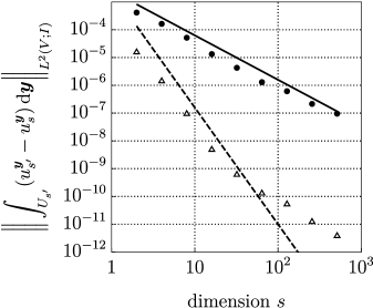
The dimension truncation errors in Theorem 6.4 are estimated by approximating the quantities
as well as
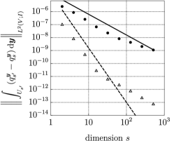
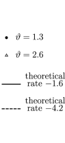
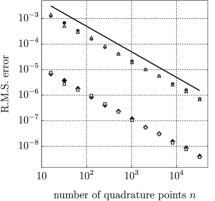
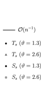
for , by using a tailored lattice cubature rule generated using the fast CBC algorithm with nodes and a single fixed random shift to compute the high-dimensional parametric integrals. The obtained results are displayed in Figures 1 and 2 for the fluctuations corresponding to decay rates and dimensions . We use in the computations corresponding to and . As the reference solution, we use the solutions corresponding to dimension .
The theoretical dimension truncation rate is readily observed in the case . We note in the case that the dimension truncation convergence rates degenerate for large values of , which is possibly due to the fact that the QMC cubature with nodes has an error around (see Figure 3 in Subsection 7.2). For smaller values of , the higher order convergence is also apparent in the case .
Figure 1: The approximate dimension truncation errors corresponding to the state and adjoint PDEs.
Figure 2: The approximate dimension truncation errors corresponding to and .
7.2 QMC error
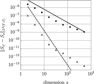
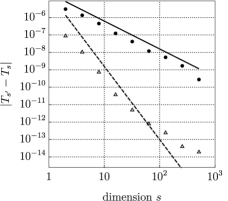
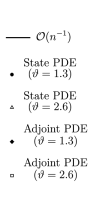
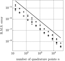
We investigate the QMC error rate by computing the root-mean-square approximations
corresponding to (6.15)–(6.18), where and are as in (6.10) for a randomly shifted lattice rule with cubature nodes (6.9), where the random shift is drawn from . As the generating vector, we use lattice rules constructed using the fast CBC algorithm with , , lattice points and random shifts, and . We carry out the experiments using two different decay rates for the input random field. The results are displayed in Figure 3. The root-mean-square error converges at a linear rate in all experiments, which is consistent with the theory.
Figure 3: Left: The approximate root-mean-square error for QMC approximation of the integrals and . Right: The approximate root-mean-square error for QMC approximation of quantities and . All computations were carried out using random shifts, , , and dimension .
We consider the problem of finding the optimal control
that minimizes (2) subject to the PDE
constraint (2.2). We consider constrained optimization over and compare our results with the reconstruction obtained by carrying out unconstrained optimization over . To this end, we define the projection operator
which is used in the constrained setting, while in the unconstrained setting we use .
To be able to handle elements of numerically, we apply the projected gradient method (see, e.g., [24]) as described in Algorithm 1 together with the projected Armijo rule stated in Algorithm 2. Note that evaluating and in Algorithms 1 and 2 requires solving the state PDE with the source term . In particular, the Riesz operator appears in the loading term after finite element discretization and can thus be evaluated using (2.4). We use the initial guess . The parameters of the gradient descent method were chosen to be , , and .
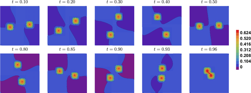
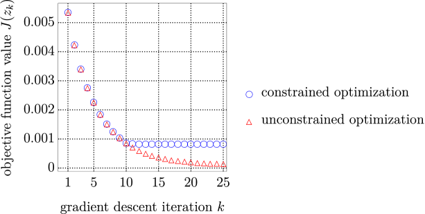
We consider the entropic risk measure with . The reconstructed optimal control obtained using the bounded set of feasible controls is displayed in Figure 4. The reconstructed optimal control at the terminal time and its pointwise difference to the control obtained without imposing control constraints are displayed in Figure 5. Finally, the evolution of the objective functional as the number of gradient descent iterations increases is plotted in Figure 6 for the constrained and unconstrained optimization problems.
Figure 4: The inverse Riesz transform of the reconstructed optimal control using the entropic risk measure for several values of in the constrained setting.
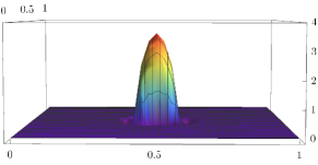
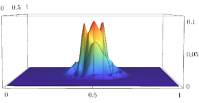
Figure 5: Left: the inverse Riesz transform of the control at time in the constrained setting after 25 iterations of the projected gradient descent algorithm using the entropic risk measure. Right: The difference between the reconstruction obtained in the constrained setting and the corresponding solution in the unconstrained setting.Figure 6: The value of the objective functional for each gradient descent iteration. The results corresponding to the constrained setting and the unconstrained setting are plotted in blue and red, respectively.
8 Conclusion
We developed a specially designed QMC method for an optimal control problem subject to a parabolic PDE with an uncertain diffusion coefficient. To account for the uncertainty, we considered as measures of risk the expected value and the more conservative (nonlinear) entropic risk measure. For the high-dimensional integrals originating from the risk measures, we provide error bounds and convergence rates in terms of dimension truncation and the QMC approximation. In particular, after dimension truncation, the QMC error bounds do not depend on the number of uncertain variables, while leading to faster convergence rates compared to Monte Carlo methods. In addition we extended QMC error bounds in the literature to separable Banach spaces, and hence the presented error analysis is discretization invariant.
Acknowledgements
P. A. Guth is grateful to the DFG RTG1953 “Statistical Modeling of Complex Systems and Processes” for funding of this research. F. Y. Kuo and I. H. Sloan acknowledge the support from the Australian Research Council (DP21010083).
References
[1]
Ph. Artzner, F. Delbaen, J.-M. Eber, and D. Heath.
Coherent measures of risk.
Math. Finance, 9:203–228, 2001.
[2]
P. Blondeel, P. Robbe, C. Van hoorickx, S. François, G. Lombaert, and
S. Vandewalle.
-refined multilevel quasi-Monte Carlo for Galerkin finite
element methods with applications in civil engineering.
Algorithms, 13(5):110, 2020.
[3]
G. Castiglione, A. Frosini, E. Munarini, A. Restivo, and S. Rinaldi.
Combinatorial aspects of -convex polyominoes.
European J. Combin., 28(6):1724–1741, 2007.
[4]
P. Chen and O. Ghattas.
Taylor approximation for chance constrained optimization problems
governed by partial differential equations with high-dimensional random
parameters.
SIAM/ASA J. Uncertain. Quantif., 9(4):1381–1410, 2021.
[5]
P. Chen and J. O. Royset.
Performance bounds for PDE-constrained optimization under
uncertainty, 2021.
Preprint at https://arxiv.org/abs/2110.10269v2.
[6]
P. Chen, U. Villa, and O. Ghattas.
Taylor approximation and variance reduction for PDE-constrained
optimal control under uncertainty.
J. Comput. Phys., 385:163–186, 2019.
[7]
A. Cohen, R. DeVore, and Ch. Schwab.
Convergence rates of best -term Galerkin approximations for a
class of elliptic sPDEs.
Found. Comput. Math., 6(10):615–646, 2010.
[8]
R. Dautray and J.-L. Lions.
Mathematical Analysis and Numerical Methods for Science and
Technology: Volume 5 Evolution Problems I.
Springer, Heidelberg, 2012.
[9]
J. Dick, R. N. Gantner, Q. T. Le Gia, and Ch. Schwab.
Higher order quasi-Monte Carlo integration for Bayesian PDE
inversion.
Comput. Math. Appl., 77(1):144–172, 2019.
[10]
J. Dick, F. Y. Kuo, and I. H. Sloan.
High-dimensional integration: The quasi-Monte Carlo way.
Acta Numer., 22:133–288, 2013.
[11]
L. C. Evans.
Partial Differential Equations.
American Mathematical Society, Providence, Rhode Island, 2010.
[12]
H. Föllmer and A. Schied.
Convex measures of risk and trading constraints.
Finance Stoch., 6:429–447, 2002.
[13]
R. N. Gantner.
Dimension truncation in QMC for affine-parametric operator
equations.
In A. B. Owen and P. W. Glynn, editors, Monte Carlo and
Quasi-Monte Carlo Methods 2016, pages 249–264, Stanford, CA, 2018.
Springer.
[14]
R. N. Gantner, L. Herrmann, and Ch. Schwab.
Quasi–Monte Carlo integration for affine-parametric, elliptic
PDEs: Local supports and product weights.
SIAM J. Numer. Anal., 56(1):111–135, 2018.
[15]
S. Garreis, T. M. Surowiec, and M. Ulbrich.
An interior-point approach for solving risk-averse PDE-constrained
optimization problems with coherent risk measures.
SIAM J. Optim., 31(1):1–29, 2021.
[16]
A. D. Gilbert, I. G. Graham, F. Y. Kuo, R. Scheichl, and I. H. Sloan.
Analysis of quasi-Monte Carlo methods for elliptic eigenvalue
problems with stochastic coefficients.
Numer. Math., 142(4):863–915, 2019.
[17]
A. D. Gilbert and R. Scheichl.
Multilevel quasi-Monte Carlo for random elliptic eigenvalue
problems I: Regularity and error analysis, 2020.
Preprint at https://arxiv.org/abs/2010.01044v3.
[18]
H. W. Gould.
Combinatorial Identities: A Standardized Set of Tables Listing
500 Binomial Coefficient Summations.
Morgantown, 1972.
[19]
P. A. Guth, V. Kaarnioja, F. Y. Kuo, C. Schillings, and I. H. Sloan.
A quasi-Monte Carlo method for optimal control under uncertainty.
SIAM/ASA J. Uncertain. Quantif., 9(2):354–383, 2021.
[20]
P. A. Guth and A. Van Barel.
Multilevel quasi-Monte Carlo for optimization under uncertainty,
2021.
Preprint at https://arxiv.org/abs/2109.14367.
[21]
H. Harbrecht, M. Peters, and M. Siebenmorgen.
On the quasi-Monte Carlo method with Halton points for elliptic
PDEs with log-normal diffusion.
Math. Comp., 86:771–797, 2017.
[22]
L. Herrmann, M. Keller, and Ch. Schwab.
Quasi-Monte Carlo Bayesian estimation under Besov priors in
elliptic inverse problems.
Math. Comp., 90:1831–1860, 2021.
[23]
L. Herrmann and Ch. Schwab.
QMC integration for lognormal-parametric, elliptic PDEs: local
supports and product weights.
Numer. Math., 141:63–102, 2019.
[24]
M. Hinze, R. Pinnau, M. Ulbrich, and S. Ulbrich.
Optimization with PDE Constraints.
Springer, Heidelberg, 2009.
[25]
Katana, 2010.
DOI:10.26190/669X-A286.
[26]
D. P. Kouri and T. M. Surowiec.
Existence and optimality conditions for risk-averse PDE-constrained
optimization.
SIAM/ASA J. Uncertain. Quantif., 6(2):787–815, 2018.
[27]
D. P. Kouri and T. M. Surowiec.
Epi-regularization of risk measures.
Math. Oper. Res., 45(2):774–795, 2020.
[28]
D. Kressner and C. Tobler.
Low-rank tensor Krylov subspace methods for parametrized linear
systems.
SIAM J. Matrix Anal. Appl., 32(4):1288–1316, 2011.
[29]
A. Kunoth and Ch. Schwab.
Analytic regularity and GPC approximation for control problems
constrained by linear parametric elliptic and parabolic PDEs.
SIAM J. Control. Optim., 51(3):2442–2471, 2013.
[30]
F. Y. Kuo and D. Nuyens.
Application of quasi-Monte Carlo methods to elliptic PDEs with
random diffusion coefficients: A survey of analysis and implementation.
Found. Comput. Math., 16:1631–1696, 2016.
[31]
F. Y. Kuo, R. Scheichl, Ch. Schwab, I. H. Sloan, and E. Ullmann.
Multilevel quasi-Monte Carlo methods for lognormal diffusion
problems.
Math. Comp., 86:2827–2860, 2017.
[32]
F. Y. Kuo, Ch. Schwab, and I. H. Sloan.
Quasi-Monte Carlo finite element methods for a class of elliptic
partial differential equations with random coefficients.
SIAM J. Numer. Anal., 50(6):3351–3374, 2012.
[33]
M. Martin, S. Krumscheid, and F. Nobile.
Complexity analysis of stochastic gradient methods for
PDE-constrained optimal control problems with uncertain parameters.
ESAIM: Math. Model. Numer. Anal., 55(4):1599–1633, 2021.
[34]
M. Martin and F. Nobile.
PDE-constrained optimal control problems with uncertain parameters
using SAGA.
SIAM/ASA J. Uncertain. Quantif., 9(3):979–1012, 2021.
[35]
J. Quaintance and H. W. Gould.
Combinatorial Identities for Stirling Numbers: The Unpublished
Notes of H. W. Gould.
World Scientific Publishing Company, River Edge, NJ, 2015.
[36]
P. Robbe, D. Nuyens, and S. Vandewalle.
Recycling samples in the multigrid multilevel (quasi-)Monte Carlo
method.
SIAM J. Sci. Comput., 41(5):S37–S60, 2019.
[37]
W. Rudin.
Functional Analysis.
McGraw-Hill, Singapore, 1991.
[38]
T. H. Savits.
Some statistical applications of Faa di Bruno.
J. Multivariate Anal., 97(10):2131–2140, 2006.
[39]
R. Scheichl, A. M. Stuart, and A. L. Teckentrup.
Quasi-Monte Carlo and multilevel Monte Carlo methods for
computing posterior expectations in elliptic inverse problems.
SIAM/ASA J. Uncertain. Quantif., 5(1):493–518, 2017.
[40]
Ch. Schwab.
QMC Galerkin discretization of parametric operator equations.
In J. Dick, F. Y. Kuo, G. W. Peters, and I. H. Sloan, editors, Monte Carlo and Quasi-Monte Carlo Methods 2012, pages 613–629, Heidelberg,
2013. Springer.
[41]
Ch. Schwab and R. Stevenson.
Space-time adaptive wavelet methods for parabolic evolution problems.
Math. Comp., 78:1293–1318, 2009.
[42]
S. Tong, E. Vanden-Eijnden, and G. Stadler.
Extreme event probability estimation using PDE-constrained
optimization and large deviation theory, with application to tsunamis.
Commun. Appl. Math. Comput. Sci., 16(2):181–225, 2021.
[43]
F. Tröltzsch.
Optimal Control of Partial Differential Equations: Theory,
Methods and Applications.
American Mathematical Society, Providence, Rhode Island, 2010.
[44]
A. Van Barel and S. Vandewalle.
Robust optimization of PDEs with random coefficients using a
multilevel Monte Carlo method.
SIAM/ASA J. Uncertain. Quantif., 7(1):174–202, 2019.
[45]
A. Van Barel and S. Vandewalle.
MG/OPT and multilevel Monte Carlo for robust optimization of
PDEs.
SIAM J. Optim., 31(3):1850–1876, 2021.
[46]
K. Yosida.
Functional Analysis.
Springer, Heidelberg, 1980.