OpenCon: Open-world Contrastive Learning

Abstract

Machine learning models deployed in the wild naturally encounter unlabeled samples from both known and novel classes. Challenges arise in learning from both the labeled and unlabeled data, in an open-world semi-supervised manner. In this paper, we introduce a new learning framework, open-world contrastive learning (OpenCon). OpenCon tackles the challenges of learning compact representations for both known and novel classes, and facilitates novelty discovery along the way. We demonstrate the effectiveness of OpenCon on challenging benchmark datasets and establish competitive performance. On the ImageNet dataset, OpenCon significantly outperforms the current best method by 11.9% and 7.4% on novel and overall classification accuracy, respectively. Theoretically, OpenCon can be rigorously interpreted from an EM algorithm perspective—minimizing our contrastive loss partially maximizes the likelihood by clustering similar samples in the embedding space. The code is available at https://github.com/deeplearning-wisc/opencon.

1 Introduction

Modern machine learning methods have achieved remarkable success (Sun et al., 2017; Van den Oord et al., 2018; Chen et al., 2020a; Caron et al., 2020; He et al., 2020; Zheng et al., 2021; Wu et al., 2021; Cha et al., 2021; Cui et al., 2021; Jiang et al., 2021; Gao et al., 2021; Zhong et al., 2021a; Zhao & Han, 2021; Fini et al., 2021; Tsai et al., 2022; Zhang et al., 2022b; Wang et al., 2022). Noticeably, the vast majority of learning algorithms have been driven by the closed-world setting, where the classes are assumed stationary and unchanged. This assumption, however, rarely holds for models deployed in the wild. One important characteristic of open world is that the model will naturally encounter novel classes. Considering a realistic scenario, where a machine learning model for recognizing products in e-commerce may encounter brand-new products together with old products. Similarly, an autonomous driving model can run into novel objects on the road, in addition to known ones. Under the setting, the model should ideally learn to distinguish not only the known classes, but also the novel categories. This problem is proposed as open-world semi-supervised learning (Cao et al., 2022) or generalized category discovery (Vaze et al., 2022). Research efforts have only started very recently to address this important and realistic problem.

Formally, we are given a labeled training dataset $\mathcal{D}_{l}$ as well as an unlabeled dataset $\mathcal{D}_{u}$. The labeled dataset contains samples that belong to a set of known classes, while the unlabeled dataset has a mixture of samples from both the known and novel classes. In practice, such unlabeled in-the-wild data can be collected almost for free upon deploying a model in the open world, and thus is available in abundance. Under the setting, our goal is to learn distinguishable representations for both known and novel classes simultaneously. While this setting naturally suits many real-world applications, it also poses unique challenges due to: (a) the lack of clear separation between known vs. novel data in $\mathcal{D}_{u}$, and (b) the lack of supervision for data in novel classes. Traditional representation learning methods are not designed for this new setting. For example, supervised contrastive learning (SupCon) (Khosla et al., 2020) only assumes the labeled set $\mathcal{D}_{l}$, without considering the unlabeled data $\mathcal{D}_{u}$. Weakly supervised contrastive learning (Zheng et al., 2021) assumes the same classes in labeled and unlabeled data, hence remaining closed-world and less generalizable to novel samples. Self-supervised learning (Chen et al., 2020a) relies completely on the unlabeled set $\mathcal{D}_{u}$ and does not utilize the availability of the labeled dataset $\mathcal{D}_{l}$.

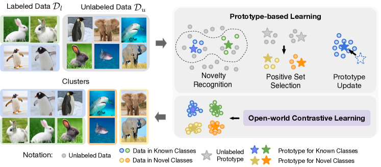
Figure 1: Illustration of our learning framework Open-world Contrastive Learning (OpenCon). The model is trained on a labeled dataset $\mathcal{D}_{l}$ of known classes, and an unlabeled dataset $\mathcal{D}_{u}$ (with samples from both known and novel classes). OpenCon aims to learn distinguishable representations for both known (blue and green) and novel (yellow and orange) classes simultaneously. See Section 3 for details.

Targeting these challenges, we formally introduce a new learning framework, open-world contrastive learning (dubbed OpenCon). OpenCon is designed to produce a compact representation space for both known and novel classes, and facilitates novelty discovery along the way. Key to our framework, we propose a novel prototype-based learning strategy, which encapsulates two components. First, we leverage the prototype vectors to separate known vs. novel classes in unlabeled data $\mathcal{D}_{u}$. The prototypes can be viewed as a set of representative embeddings, one for each class, and are updated by the evolving representations. Second, to mitigate the challenge of lack of supervision, we generate pseudo-positive pairs for contrastive comparison. We define the positive set to be those examples carrying the same approximated label, which is predicted based on the closest class prototype. In effect, the loss encourages closely aligned representations to all samples from the same predicted class, rendering a compact clustering of the representation.

Our framework offers several compelling advantages. (1) Empirically, OpenCon establishes strong performance on challenging benchmark datasets, outperforming existing baselines by a significant margin (Section 5). OpenCon is also competitive without knowing the number of novel classes in advance—achieving similar or even slightly better performance compared to the oracle (in which the number of classes is given). (2) Theoretically, we demonstrate that our prototype-based learning can be rigorously interpreted from an Expectation-Maximization (EM) algorithm perspective. (3) Our framework is end-to-end trainable, and is compatible with both CNN-based and Transformer-based architectures. Our main contributions are:

1. We propose a novel framework, open-world contrastive learning (OpenCon), tackling a largely unexplored problem in representation learning. As an integral part of our framework, we also introduce a prototype-based learning algorithm, which facilitates novelty discovery and learning distinguishable representations.

2. Empirically, OpenCon establishes competitive performance on challenging tasks. For example, on the ImageNet dataset, OpenCon substantially outperforms the current best method ORCA (Cao et al., 2022) by 11.9% and 7.4% in terms of novel and overall accuracy.

3. We provide insights through extensive ablations, showing the effectiveness of components in our framework. Theoretically, we show a formal connection with EM algorithm—minimizing our contrastive loss partially maximizes the likelihood by clustering similar samples in the embedding space.

2 Problem Setup

Table 1: Comparison of different problem settings.

Problem Setting	Labeled data	Unlabeled data
		Known classes	Novel classes
Semi-supervised learning	Yes	Yes	No
Robust semi-supervised learning	Yes	Yes	Yes (Reject)
Supervised learning	Yes	No	No
Novel class discovery	Yes	No	Yes (Discover)
Open-world Semi-supervised learning	Yes	Yes	Yes (Cluster)

The open-world setting emphasizes the fact that new classes can emerge jointly with existing classes in the wild. Formally, we describe the data setup and learning goal:

Data setup We consider the training dataset $\mathcal{D}=\mathcal{D}_{l}\cup\mathcal{D}_{u}$ with two parts:

1. The labeled set $\mathcal{D}_{l}=\left\{\mathbf{x}_{i},y_{i}\right\}_{i=1}^{n}$, with $y_{i}\in\mathcal{Y}_{l}$. The label set $\mathcal{Y}_{l}$ is known.

2. The unlabeled set $\mathcal{D}_{u}=\left\{\mathbf{x}_{i}\right\}_{i=1}^{m}$, where each sample $\mathbf{x}_{i}\in\mathcal{X}$ can come from either known or novel classes. Note that we do not have access to the labels in $\mathcal{D}_{u}$. For mathematical convenience, we denote the underlying label set as $\mathcal{Y}_{\text{all}}$, where $\mathcal{Y}_{l}\subset\mathcal{Y}_{\text{all}}$ implies category shift and expansion. Accordingly, the set of novel classes is $\mathcal{Y}_{n}=\mathcal{Y}_{\text{all}}\backslash\mathcal{Y}_{l}$, where the subscript $n$ stands for “novel”. The model has no knowledge of the set $\mathcal{Y}_{n}$ nor its size.

Goal Under the setting, the goal is to learn distinguishable representations for both known and novel classes simultaneously.

Difference w.r.t. existing problem settings Our paper addresses a practical and underexplored problem, which differs from existing problem settings (see Table 1 for a summary). In particular, (a) we consider both labeled data and unlabeled data in training, and (b) we consider a mixture of both known and novel classes in unlabeled data. Note that our setting generalizes traditional representation learning. For example, Supervised Contrastive Learning (SupCon) (Khosla et al., 2020) only assumes the labeled set $\mathcal{D}_{l}$, without considering the unlabeled data $\mathcal{D}_{u}$. Weakly supervised contrastive learning (Zheng et al., 2021) assumes the same classes in labeled and unlabeled data, i.e., $\mathcal{Y}_{l}=\mathcal{Y}_{\text{all}}$, and hence remains closed-world. Self-supervised learning (Chen et al., 2020a) relies completely on the unlabeled set $\mathcal{D}_{u}$ and does not assume the availability of the labeled dataset. The setup is also known as open-world semi-supervised learning, which is originally introduced by (Cao et al., 2022). Despite the similar setup, our learning goal is fundamentally different: Cao et al. (2022) focus on classification accuracy, but not learning high-quality embeddings. Similar to GCD Vaze et al. (2022), we aim to learning compact embeddings for both known and novel classes.

3 Proposed Method: Open-world Contrastive Learning

We formally introduce a new learning framework, open-world contrastive learning (dubbed OpenCon), which is designed to produce compact representation space for both known and novel classes. The open-world setting posits unique challenges for learning effective representations, namely due to (1) the lack of the separation between known vs. novel data in $\mathcal{D}_{u}$, (2) the lack of supervision for data in novel classes. Our learning framework targets these challenges.

3.1 Background: Generalized Contrastive Loss

We start by defining a generalized contrastive loss that can characterize the family of contrastive losses. We will later instantiate the formula to define our open-world contrastive loss (Section 3.2 and Section 3.3). Specifically, we consider a deep neural network encoder $\phi:\mathcal{X}\mapsto\mathbb{R}^{d}$ that maps the input $\mathbf{x}$ to a $L_{2}$-normalized feature embedding $\phi(\mathbf{x})$. Contrastive losses operate on the normalized feature $\mathbf{z}=\phi(\mathbf{x})$. In other words, the features have unit norm and lie on the unit hypersphere. For a given anchor point $\mathbf{x}$, we define the per-sample contrastive loss:

$$\mathcal{L}_{\phi}\big{(}\mathbf{x};\tau,\mathcal{P}(\mathbf{x}),\mathcal{N}(\mathbf{x})\big{)}=-\frac{1}{|\mathcal{P}(\mathbf{x})|}\sum_{\mathbf{z}^{+}\in\mathcal{P}(\mathbf{x})}\log\frac{\exp(\mathbf{z}^{\top}\cdot\mathbf{z}^{+}/\tau)}{\sum_{\mathbf{z}^{-}\in\mathcal{N}(\mathbf{x})}\exp(\mathbf{z}^{\top}\cdot\mathbf{z}^{-}/\tau)},$$ (1)

where $\tau$ is the temperature parameter, $\mathbf{z}$ is the $L_{2}$-normalized embedding vector of $\mathbf{x}$, $\mathcal{P}(\mathbf{x})$ is the positive set of embeddings w.r.t. $\mathbf{z}$, and $\mathcal{N}(\mathbf{x})$ is the negative set of embeddings.

In open-world contrastive learning, the crucial challenge is how to construct $\mathcal{P}(\mathbf{x})$ and $\mathcal{N}(\mathbf{x})$ for different types of samples. Recall that we have two broad categories of training data: (1) labeled data $\mathcal{D}_{l}$ with known class, and (2) unlabeled data $\mathcal{D}_{u}$ with both known and novel classes. In conventional supervised CL frameworks with $\mathcal{D}_{l}$ only, the positive sample pairs can be easily drawn according to the ground-truth labels (Khosla et al., 2020). That is, $\mathcal{P}(\mathbf{x})$ consists of embeddings of samples that carry the same label as the anchor point $\mathbf{x}$, and $\mathcal{N}(\mathbf{x})$ contains all the embeddings in the multi-viewed mini-batch excluding itself. However, this is not straightforward in the open-world setting with novel classes.

3.2 Learning from Wild Unlabeled Data

We now dive into the most challenging part of the data, $\mathcal{D}_{u}$, which contains both known and novel classes. We propose a novel prototype-based learning strategy that tackles the challenges of: (1) the separation between known and novel classes in $\mathcal{D}_{u}$, and (2) pseudo label assignment that can be used for positive set construction for novel classes. Both components facilitate the goal of learning compact representations, and enable end-to-end training.

Key to our framework, we keep a prototype embedding vector $\boldsymbol{\mu}_{c}$ for each class $c\in\mathcal{Y}_{\text{all}}$. Here $\mathcal{Y}_{\text{all}}$ contains both known classes $\mathcal{Y}_{l}$ and novel classes $\mathcal{Y}_{n}=\mathcal{Y}_{\text{all}}\backslash\mathcal{Y}_{l}$, and $\mathcal{Y}_{l}\cap\mathcal{Y}_{n}=\emptyset$. The prototypes can be viewed as a set of representative embedding vectors. All the prototype vectors $\mathbf{M}=[\boldsymbol{\mu}_{1}|...|\boldsymbol{\mu}_{c}|...]_{c\in\mathcal{Y}_{\text{all}}}$ are randomly initiated at the beginning of training, and will be updated along with learned embeddings. We will also discuss determining the cardinality $|\mathcal{Y}_{\text{all}}|$ (i.e., number of prototypes) in Section 6.

Prototype-based OOD detection

We leverage the prototype vectors to perform out-of-distribution (OOD) detection, i.e., separate known vs. novel data in $\mathcal{D}_{u}$. For any given sample $\mathbf{x}_{i}\in\mathcal{D}_{u}$, we measure the cosine similarity between its embedding $\phi(\mathbf{x}_{i})$ and prototype vectors of known classes $\mathcal{Y}_{l}$. If the sample embedding is far away from all the known class prototypes, it is more likely to be a novel sample, and vice versa. Formally, we propose the level set estimation:

$$\mathcal{D}_{n}=\{\mathbf{x}_{i}|\underset{j\in\mathcal{Y}_{l}}{\max}~{}~{}~{}\boldsymbol{\mu}_{j}^{\top}\cdot\phi(\mathbf{x}_{i})<\lambda\},$$ (2)

where a thresholding mechanism is exercised to distinguish between known and novel samples during training time. The threshold $\lambda$ can be chosen based on the labeled data $\mathcal{D}_{l}$. Specifically, one can calculate the scores $\max_{j\in\mathcal{Y}_{l}}\boldsymbol{\mu}_{j}^{\top}\cdot\phi(\mathbf{x}_{i})$ for all the samples in $\mathcal{D}_{l}$, and use the score at the $p$-percentile as the threshold. For example, when $p=90$, that means 90% of labeled data is above the threshold. We provide ablation on the effect of $p$ later in Section 6 and theoretical insights into why OOD detection helps open-world representation learning in Appendix D.

Positive and negative set selection

Now that we have identified novel samples from the unlabeled sample, we would like to facilitate learning compact representations for $\mathcal{D}_{n}$, where samples belonging to the same class are close to each other. As mentioned earlier, the crucial challenge is how to construct the positive set, denoted as $\mathcal{P}_{n}(\mathbf{x})$. In particular, we do not have any supervision signal for unlabeled data in the novel classes. We propose utilizing the predicted label $\hat{y}=\text{argmax}_{j\in\mathcal{Y}_{\text{all}}}\boldsymbol{\mu}_{j}^{\top}\cdot\phi(\mathbf{x})$ for positive set selection.

For a mini-batch $\mathcal{B}_{n}$ with samples drawn from $\mathcal{D}_{n}$, we apply two random augmentations for each sample and generate a multi-viewed batch $\tilde{\mathcal{B}}_{n}$. We denote the embeddings of the multi-viewed batch as $\mathcal{A}_{n}$, where the cardinality $|\mathcal{A}_{n}|=2|\mathcal{B}_{n}|$. For any sample $\mathbf{x}$ in the mini-batch $\tilde{\mathcal{B}}_{n}$, we propose selecting the positive and negative set of embeddings as follows:

$$\mathcal{P}_{n}(\mathbf{x}) =\{\mathbf{z}^{\prime}|\mathbf{z}^{\prime}\in\{\mathcal{A}_{n}\backslash\mathbf{z}\},\hat{y}^{\prime}=\hat{y}\},$$ (3)

$$\mathcal{N}_{n}(\mathbf{x}) =\mathcal{A}_{n}\backslash\mathbf{z},$$ (4)

where $\mathbf{z}$ is the $L_{2}$-normalized embedding of $\mathbf{x}$, and $\hat{y}^{\prime}$ is the predicted label for the corresponding training example of $\mathbf{z}^{\prime}$. In other words, we define the positive set of $\mathbf{x}$ to be those examples carrying the same approximated label prediction $\hat{y}$.

With the positive and negative sets defined, we are now ready to introduce our new contrastive loss for open-world data. We desire embeddings where samples assigned with the same pseudo-label can form a compact cluster. Following the general template in Equation 1, we define a novel loss function:

$$\mathcal{L}_{n}=\sum_{\mathbf{x}\in\tilde{\mathcal{B}}_{n}}\mathcal{L}_{\phi}\big{(}\mathbf{x};\tau_{n},\mathcal{P}_{n}(\mathbf{x}),\mathcal{N}_{n}(\mathbf{x})\big{)}.$$ (5)

For each anchor, the loss encourages the network to align embeddings of its positive pairs while repelling the negatives. All positives in a multi-viewed batch (i.e., the augmentation-based sample as well as any of the remaining samples with the same label) contribute to the numerator. The loss encourages the encoder to give closely aligned representations to all entries from the same predicted class, resulting in a compact representation space. We provide visualization in Figure 2 (right).

Prototype update

The most canonical way to update the prototype embeddings is to compute it in every iteration of training. However, this would extract a heavy computational toll and in turn cause unbearable training latency. Instead, we update the class-conditional prototype vector in a moving-average style (Li et al., 2020; Wang et al., 2022):

$$\boldsymbol{\mu}_{c}:=\operatorname{Normalize}\left(\gamma\boldsymbol{\mu}_{c}+(1-\gamma)\mathbf{z}\right),\text{for}~{}c=\begin{cases}y\text{ (ground truth label)},&\text{if }\mathbf{z}\in\mathcal{D}_{l}\\ \text{argmax}_{j\in\mathcal{Y}_{\text{n}}}\boldsymbol{\mu}_{j}^{\top}\cdot\mathbf{z},&\text{if }\mathbf{z}\in\mathcal{D}_{n}\end{cases}$$ (6)

Here, the prototype $\boldsymbol{\mu}_{c}$ of class $c$ is defined by the moving average of the normalized embeddings $\mathbf{z}$, whose predicted class conforms to $c$. $\mathbf{z}$ are embeddings of samples from $\mathcal{D}_{l}\cup\mathcal{D}_{n}$. $\gamma$ is a tunable hyperparameter.

Remark: We exclude samples in $\mathcal{D}_{u}\backslash\mathcal{D}_{n}$ because they may contain non-distinguishable data from known and unknown classes, which undesirably introduce noise to the prototype estimation. We verify this phenomenon by comparing the performance of mixing $\mathcal{D}_{u}\backslash\mathcal{D}_{n}$ with labeled data $\mathcal{D}_{l}$ for training the known classes. The results verify our hypothesis that the non-distinguishable data would be harmful to the overall accuracy. We provide more discussion on this in Appendix E.

3.3 Open-world Contrastive Loss

Putting it all together, we define the open-world contrastive loss (dubbed OpenCon) as the following:

$$\mathcal{L}_{\text{OpenCon}}=\lambda_{n}\mathcal{L}_{n}+\lambda_{l}\mathcal{L}_{l}+\lambda_{u}\mathcal{L}_{u},$$ (7)

where $\mathcal{L}_{n}$ is the newly devised contrastive loss for the novel data, $\mathcal{L}_{l}$ is the supervised contrastive loss (Khosla et al., 2020) employed on the labeled data $\mathcal{D}_{l}$, and $\mathcal{L}_{u}$ is the self-supervised contrastive loss (Chen et al., 2020a) employed on the unlabeled data $\mathcal{D}_{u}$. $\lambda$ are the coefficients of loss terms. Details of $\mathcal{L}_{l}$ and $\mathcal{L}_{u}$ are in Appendix B, along with the complete pseudo-code in Algorithm 1 (Appendix).

Remark

Our loss components work collaboratively to enhance the embedding quality in an open-world setting. The overall objective well suits the complex nature of our training data, which blends both labeled and unlabeled data. As we will show later in Section 6, a simple solution by combining supervised contrastive loss (on labeled data) and self-supervised loss (on unlabeled data) is suboptimal. Instead, having $\mathcal{L}_{n}$ is critical to encourage closely aligned representations to all entries from the same predicted class, resulting in an overall more compact representation for novel classes.

4 Theoretical Understandings

Overview

Our learning objective using wild data (c.f. Section 3.2) can be rigorously interpreted from an Expectation-Maximization (EM) algorithm perspective. We start by introducing the high-level ideas of how our method can be decomposed into E-step and M-step respectively. At the E-step, we assign each data example $\mathbf{x}\in\mathcal{D}_{n}$ to one specific cluster. In OpenCon, it is estimated by using the prototypes: $\hat{y}_{i}=\text{argmax}_{j\in\mathcal{Y}_{\text{all}}}\boldsymbol{\mu}_{j}^{\top}\cdot\phi(\mathbf{x}_{i})$. At the M-step, the EM algorithm aims to maximize the likelihood under the posterior class probability from the previous E-step. Theoretically, we show that minimizing our contrastive loss $\mathcal{L}_{n}$ (Equation 5) partially maximizes the likelihood by clustering similar examples. In effect, our loss concentrates similar data to the corresponding prototypes, encouraging the compactness of features.

4.1 Analyzing the E-step

In E-step, the goal of the EM algorithm is to maximize the likelihood with learnable feature encoder $\phi$ and prototype matrix $\mathbf{M}=[\boldsymbol{\mu}_{1}|...|\boldsymbol{\mu}_{c}|...]$, which can be lower bounded:

$$\sum_{i}^{|\mathcal{D}_{n}|}\operatorname{log}p(\mathbf{x}_{i}|\phi,\mathbf{M})\geq\sum_{i}^{|\mathcal{D}_{n}|}q_{i}(c)\operatorname{log}\sum_{c\in\mathcal{Y}_{\text{all}}}\frac{p(\mathbf{x}_{i},c|\phi,\mathbf{M})}{q_{i}(c)},$$

where $q_{i}(c)$ is denoted as the density function of a possible distribution over $c$ for sample $\mathbf{x}_{i}$. By using the fact that $\log(\cdot)$ function is concave, the inequality holds with equality when $\frac{p(\mathbf{x}_{i},c|\phi,\mathbf{M})}{q_{i}(c)}$ is a constant value, therefore we set:

$$q_{i}(c)=\frac{p(\mathbf{x}_{i},c|\phi,\mathbf{M})}{\sum_{c\in\mathcal{Y}_{\text{all}}}p(\mathbf{x}_{i},c|\phi,\mathbf{M})}=\frac{p(\mathbf{x}_{i},c|\phi,\mathbf{M})}{p(\mathbf{x}_{i}|\phi,\mathbf{M})}=p(c|\mathbf{x}_{i},\phi,\mathbf{M}),$$

which is the posterior class probability. To estimate $p(c|\mathbf{x}_{i},\phi,\mathbf{M})$, we model the data using the von Mises-Fisher (vMF) (Fisher, 1953) distribution since the normalized embedding locates in a high-dimensional hyperspherical space.

Assumption 4.1.

The density function is given by $f\left(\mathbf{x}|\boldsymbol{\mu},\kappa\right)=c_{d}(\kappa)e^{\kappa\boldsymbol{\mu}^{\top}\phi(\mathbf{x})}$, where $\kappa$ is the concentration parameter and $c_{d}(\kappa)$ is a coefficient.

With the vMF distribution assumption in  4.1, we have $p(c|\mathbf{x}_{i},\phi,\mathbf{M})=\sigma_{c}(\mathbf{M}^{\top}\cdot\phi(\mathbf{x}_{i})),$ where $\sigma$ denotes the softmax function and $\sigma_{c}$ is the $c$-th element. Empirically we take a one-hot prediction with $\hat{y}_{i}=\text{argmax}_{j\in\mathcal{Y}_{\text{all}}}\boldsymbol{\mu}_{j}^{\top}\cdot\phi(\mathbf{x}_{i})$ since each example inherently belongs to exactly one prototype, so we let $q_{i}(c)=\mathbf{1}\{c=\hat{y}_{i}\}$.

4.2 Analyzing the M-step

In M-step, using the label distribution prediction $q_{i}(c)$ in the E-step, the optimization for the network $\phi$ and the prototype matrix $\mathbf{M}$ is given by:

$$\underset{\phi,\mathbf{M}}{\operatorname{argmax\ }}\sum_{i=1}^{|\mathcal{D}_{n}|}\sum_{c\in\mathcal{Y}_{\text{all}}}q_{i}(c)\log\frac{p\left(\mathbf{x}_{i},c|\phi,\mathbf{M}\right)}{q_{i}(c)}$$ (8)

The joint optimization target in Equation 8 is then achieved by rewriting the Equation 8 according to the following Lemma 4.2 with proof in Appendix F:

Lemma 4.2.

(Zha et al., 2001) We define the set of samples with the same prediction $\mathcal{S}(c)=\{\mathbf{x}_{i}\in\mathcal{D}_{n}|\hat{y}_{i}=c\}$. The maximization step is equivalent to aligning the feature vector $\phi(\mathbf{x})$ to the corresponding prototype $\boldsymbol{\mu}_{c}$:

$$\underset{\phi,\mathbf{M}}{\operatorname{argmax\ }}\sum_{i=1}^{|\mathcal{D}_{n}|}\sum_{c\in\mathcal{Y}_{\text{all}}}q_{i}(c)\log\frac{p\left(\mathbf{x}_{i},c|\phi,\mathbf{M}\right)}{q_{i}(c)} =\underset{\phi,\mathbf{M}}{\operatorname{argmax\ }}\sum_{c\in\mathcal{Y}_{\text{all}}}\sum_{\mathbf{x}\in\mathcal{S}(c)}\phi(\mathbf{x})^{\top}\cdot\boldsymbol{\mu}_{c}$$

In our algorithm, the maximization step is achieved by optimizing $\mathbf{M}$ and $\phi$ separately.

(a) Optimizing $\mathbf{M}$:

For fixed $\phi$, the optimal prototype is given by $\boldsymbol{\mu}^{*}_{c}=\operatorname{Normalize}(\mathbb{E}_{\mathbf{x}\in\mathcal{S}(c)}[\phi(\mathbf{x})]).$ This optimal form empirically corresponds to our prototype estimation in Equation 6. Empirically, it is expensive to collect all features in $\mathcal{S}(c)$. We use the estimation of $\boldsymbol{\mu}_{c}$ by moving average: $\boldsymbol{\mu}_{c}:=\operatorname{Normalize}\left(\gamma\boldsymbol{\mu}_{c}+(1-\gamma)\phi(\mathbf{x})\right),\forall\mathbf{x}\in\mathcal{S}(c)$.

(b) Optimizing $\phi$:

We then show that the contrastive loss $\mathcal{L}_{n}$ composed with the alignment loss part $\mathcal{L}_{a}$ encourages the closeness of features from positive pairs. By minimizing $\mathcal{L}_{a}$, it is approximately maximizing the target in Equation 8 with the optimal prototypes $\boldsymbol{\mu}_{c}^{*}$. We can decompose the loss as follows:

$$\mathcal{L}_{n} =-\frac{1}{|\mathcal{P}(\mathbf{x})|}\sum_{\mathbf{z}^{+}\in\mathcal{P}(\mathbf{x})}\log\frac{\exp(\mathbf{z}^{\top}\cdot\mathbf{z}^{+}/\tau)}{\sum_{\mathbf{z}^{-}\in\mathcal{N}(\mathbf{x})}\exp(\mathbf{z}\cdot\mathbf{z}^{-}/\tau)}$$

$$=\underbrace{-\frac{1}{|\mathcal{P}(\mathbf{x})|}\sum_{\mathbf{z}^{+}\in\mathcal{P}(\mathbf{x})}(\mathbf{z}^{\top}\cdot\mathbf{z}^{+}/\tau)}_{\mathcal{L}_{a}(\mathbf{x})}+\underbrace{\frac{1}{|\mathcal{P}(\mathbf{x})|}\sum_{\mathbf{z}^{+}\in\mathcal{P}(\mathbf{x})}\log\sum_{\mathbf{z}^{-}\in\mathcal{N}(\mathbf{x})}\exp(\mathbf{z}^{\top}\cdot\mathbf{z}^{-}/\tau)}_{\mathcal{L}_{b}(\mathbf{x})}.$$

In particular, the first term $\mathcal{L}_{a}(\mathbf{x})$ is referred to as the alignment term  (Wang & Isola, 2020), which encourages the compactness of features from positive pairs. To see this, we have the following lemma 4.3 with proof in Appendix F.

Lemma 4.3.

Minimizing $\mathcal{L}_{a}(\mathbf{x})$ is equivalent to the maximization step w.r.t. parameter $\phi$.

$$\underset{\phi}{\operatorname{argmin\ }}\sum_{\mathbf{x}\in\mathcal{D}_{n}}\mathcal{L}_{a}(\mathbf{x}) =\underset{\phi}{\operatorname{argmax\ }}\sum_{c\in\mathcal{Y}_{\text{all}}}\sum_{\mathbf{x}\in\mathcal{S}(c)}\phi(\mathbf{x})^{\top}\cdot\boldsymbol{\mu}^{*}_{c},$$

Summary

These observations validate that our framework learns representation for novel classes in an EM fashion. Importantly, we extend EM from a traditional learning setting to an open-world setting with the capability to handle real-world data arising in the wild. We proceed by introducing the empirical verification of our algorithm.

5 Experimental Results

Datasets We evaluate on standard benchmark image classification datasets CIFAR-100 (Krizhevsky et al., 2009) and ImageNet (Deng et al., 2009). For the ImageNet, we sub-sample 100 classes, following the same setting as ORCA (Cao et al., 2022) for fair comparison. Results on ImageNet-1k is also provided in Appendix L. Note that we focus on these tasks, as they are much more challenging than toy datasets with fewer classes. The additional comparison on CIFAR-10 is in Appendix G. By default, classes are divided into 50% seen and 50% novel classes. We then select 50% of known classes as the labeled dataset, and the rest as the unlabeled set. The division is consistent with Cao et al. (2022), which allows us to compare the performance in a fair setting. Additionally, we explore different ratios of unlabeled data and novel classes (see Section 6).

Evaluation metrics We follow the evaluation strategy in Cao et al. (2022) and report the following metrics: (1) classification accuracy on known classes, (2) classification accuracy on the novel data, and (3) overall accuracy on all classes. The accuracy of the novel classes is measured by solving an optimal assignment problem using the Hungarian algorithm (Kuhn & Yaw, 1955). When reporting accuracy on all classes, we solve optimal assignments using both known and novel classes.

Experimental details We use ResNet-18 as the backbone for CIFAR-100 and ResNet-50 as the backbone for ImageNet-100. The pre-trained backbones (no final FC layer) are identical to the ones in  Cao et al. (2022). To ensure a fair comparison, we follow the same practice in Cao et al. (2022) and only update the parameters of the last block of ResNet. In addition, we add a trainable two-layer MLP projection head that projects the feature from the penultimate layer to a lower-dimensional space $\mathbb{R}^{d}$ ($d=128$), which is shown to be effective for contrastive loss (Chen et al., 2020a). We use the same data augmentation strategies as SimCLR (Chen et al., 2020a). Same as in  Cao et al. (2022), we regularize the KL-divergence between the predicted label distribution $p\left(\hat{y}\right)$ and the class prior to prevent the network degenerating into a trivial solution in which all instances are assigned to a few classes. We provide extensive details on the training configurations and all hyper-parameters in Appendix I.

Table 2: Main Results. Asterisk (^⋆) denotes that the original method can not recognize seen classes. Dagger (^†) denotes the original method can not detect novel classes (and we had to extend it). Results on ORCA, GCD and OpenCon (mean and standard deviation) are averaged over five different runs. The ORCA results are reported based on the official repo (Cao et al., ).

Method	CIFAR-100			ImagNet-100
	All	Novel	Seen	All	Novel	Seen
†FixMatch (Kurakin et al., 2020)	20.3	23.5	39.6	34.9	36.7	65.8
†DS3L (Guo et al., 2020)	24.0	23.7	55.1	30.8	32.5	71.2
†CGDL (Sun et al., 2020)	23.6	22.5	49.3	31.9	33.8	67.3
⋆DTC (Han et al., 2019)	18.3	22.9	31.3	21.3	20.8	25.6
⋆RankStats (Zhao & Han, 2021)	23.1	28.4	36.4	40.3	28.7	47.3
⋆SimCLR (Chen et al., 2020a)	22.3	21.2	28.6	36.9	35.7	39.5
ORCA (Cao et al., 2022)	47.2±0.7	41.0±1.0	66.7±0.2	76.4±1.3	68.9±0.8	89.1±0.1
GCD (Vaze et al., 2022)	46.8±0.5	43.4±0.7	69.7±0.4	75.5±1.4	72.8±1.2	90.9 ±0.2
OpenCon (Ours)	52.7±0.6	47.8±0.6	69.1±0.3	83.8±0.3	80.8±0.3	90.6±0.1

OpenCon achieves SOTA performance As shown in Table 1, OpenCon outperforms the rivals by a significant margin on both CIFAR and ImageNet datasets. Our comparison covers an extensive collection of algorithms, including the best-performed methods to date. In particular, on ImageNet-100, we improve upon the best baseline by 7.4% in terms of overall accuracy. It is also worth noting that OpenCon improves the accuracy of novel classes by 11.9%. Note that the open-world representation learning is a relatively new setting. Closest to our setting is the open-world semi-supervised learning (SSL) algorithms, namely ORCA (Cao et al., 2022) and GCD (Vaze et al., 2022)—that directly optimize the classification performance. While our framework emphasizes representation learning, we demonstrate the quality of learned embeddings by also measuring the classification accuracy. This can be easily done by leveraging our learned prototypes on a converged model: $\hat{y}=\text{argmax}_{j\in\mathcal{Y}_{\text{all}}}~{}\boldsymbol{\mu}_{j}^{\top}\cdot\phi(\mathbf{x})$. We discuss the significance w.r.t. existing works in detail:

• OpenCon vs. ORCA Our framework bears significant differences w.r.t. ORCA in terms of learning goal and approach. (1) Our framework focuses on the representation learning problem, whereas ORCA optimizes for the classification performance using cross-entropy loss. Unlike ours, ORCA does not necessarily learn compact representations, as evidenced in Figure 2 (left). (2) We propose a novel open-world contrastive learning framework, whereas ORCA does not employ contrastive learning. ORCA uses a pairwise loss to predict similarities between pairs of instances, and does not consider negative samples. In contrast, our approach constructs both positive and negative sample sets, which encourage aligning representations to all entries from the same ground-truth label or predicted pseudo label (for novel classes). (3) Our framework explicitly considers OOD detection, which allows separating known vs. novel data in $\mathcal{D}_{u}$. ORCA does not consider this and can suffer from noise in the pairwise loss (e.g., the loss may maximize the similarity between samples from known vs. novel classes).

• OpenCon vs. GCD There are two key differences to highlight: (1) GCD (Vaze et al., 2022) requires a two-stage training procedure, whereas our learning framework proposes an end-to-end training strategy. Specifically, GCD applies the SupCon loss (Khosla et al., 2020) on the labeled data $\mathcal{D}_{l}$ and SimCLR loss (Chen et al., 2020a) on the unlabeled data $\mathcal{D}_{u}$. The feature is then clustered separately by a semi-supervised K-means method. However, the two-stage method hinders the useful pseudo-labels to be incorporated into the training stage, which results in suboptimal performance. In contrast, our prototype-based learning strategy alleviates the need for a separate clustering process (c.f. Section 3.2), which is therefore easy to use in practice and provides meaningful supervision for the unlabeled data. (2) We propose a contrastive loss $\mathcal{L}_{n}$ better utilizing the pseudo-labels during training, which facilitates learning a more compact representation space for the novel data . From Table 2, we observe that OpenCon outperforms GCD by 8.3% (overall accuracy) on ImageNet-100, showcasing the benefits of our framework.

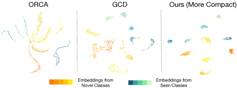
Figure 2: UMAP (McInnes et al., 2018) visualization of the feature embedding from 10 classes (5 for seen, 5 for novel) when the model is trained on ImageNet-100 with ORCA (Cao et al., 2022), GCD (Vaze et al., 2022) and OpenCon (ours).

Lastly, for completeness, we compare methods in related problem domains: (1) novel class detection: dtc (Han et al., 2019), RankStats (Zhao & Han, 2021), (2) semi-supervised learning: FixMatch (Kurakin et al., 2020), ds³l (Guo et al., 2020) and cgdl (Sun et al., 2020). We also compare it with the common representation method SimCLR (Chen et al., 2020a). These methods are not designed for the Open-SSL task, therefore the performance is less competitive.

Table 3: Comparison of accuracy on ViT-B/16 architecture (Dosovitskiy et al., 2020). Results are reported on ImageNet-100.

Methods	All	Novel	Seen
ORCA (Cao et al., 2022)	73.5	64.6	89.3
GCD (Vaze et al., 2022)	74.1	66.3	89.8
$k$-Means (MacQueen, 1967)	72.7	71.3	75.5
RankStats+ (Zhao & Han, 2021)	37.1	24.8	61.6
UNO+ (Fini et al., 2021)	70.3	57.9	95.0
OpenCon (Ours)	84.0	81.2	93.8

OpenCon is competitive on ViT Going beyond convolutional neural networks, we show in Table 3 that the OpenCon is competitive for transformer-based ViT model (Dosovitskiy et al., 2020). We adopt the ViT-B/16 architecture with DINO pre-trained weights  (Caron et al., 2021), following the pipeline used in  Vaze et al. (2022). In Table 3, we compare OpenCon’s performance with ORCA (Cao et al., 2022), GCD (Vaze et al., 2022), $k$-Means (MacQueen, 1967), RankStats+ (Zhao & Han, 2021) and UNO+ (Fini et al., 2021) on ViT-B-16 architecture. On ImageNet-100, we improve upon the best baseline by 9.9 in terms of overall accuracy.

OpenCon learns more distinguishable representations We visualize feature embeddings using UMAP (McInnes et al., 2018) in Figure 2. Different colors represent different ground-truth class labels. For clarity, we use the ImageNet-100 dataset and visualize a subset of 10 classes. We can observe that OpenCon produces a better embedding space than GCD and ORCA. In particular, ORCA does not produce distinguishable representations for novel classes, especially when the number of classes increases. The features of GCD are improved, yet with some class overlapping (e.g., two orange classes). For reader’s reference, we also include the version with a subset of 20 classes in Appendix H, where OpenCon displays more distinguishable representations.

6 A Comprehensive Analysis of OpenCon

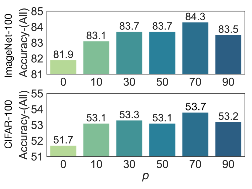
Figure 3: Effect of $p$ on ImageNet-100 and CIFAR-100, measured by the overall accuracy. $p=0$ means no OOD detection.

Prototype-based OOD detection is important In Figure 3, we ablate the contribution of a key component in OpenCon: prototype-based OOD detection (c.f. Section 3.2). To systematically analyze the effect, we report the performance under varying percentile $p\in\{0,10,30,50,70,90\}$. Each $p$ corresponds to a different threshold $\lambda$ for separating known vs. novel data in $\mathcal{D}_{u}$. In the extreme case with $p=0$, $\mathcal{D}_{n}$ becomes equivalent to $\mathcal{D}_{u}$, and hence the contrastive loss $\mathcal{L}_{n}$ is applied to the entire unlabeled data. We highlight two findings: (1) Without OOD detection ($p=0$), the unseen accuracy reduces by 2.4%, compared to the best setting ($p=70\%$). This affirms the importance of OOD detection for better representation learning. (2) A higher percentile $p$, in general, leads to better performance. We also provide theoretical insights in Appendix D showing OOD detection helps contrastive learning of novel classes by having fewer candidate classes.

Table 4: Ablation study on loss component.

Loss Components	CIFAR-100			ImageNet-100
	All	Novel	Seen	All	Novel	Seen
w/o $\mathcal{L}_{l}$	43.3	47.1	38.8	68.6	73.4	59.1
w/o $\mathcal{L}_{u}$	36.9	28.3	63.4	55.9	39.3	89.2
w/o $\mathcal{L}_{n}$	46.6	42.2	70.3	74.5	70.7	91.0
OpenCon (ours)	52.7±0.6	47.8±0.6	69.1±0.3	83.8±0.3	80.8±0.3	90.6±0.1

Ablation study on the loss components

Recall that our overall objective function in Equation 7 consists of three parts. We ablate the contributions of each component in Table 4. Specifically, we modify OpenCon by removing: (i) supervised objective (i.e., w/o $\mathcal{D}_{l}$), (ii) unsupervised objective on the entire unlabeled data (i.e., w/o $\mathcal{D}_{u}$), and (iii) prototype-based contrastive learning on novel data $\mathcal{D}_{n}$. We have the following key observations: (1) Both supervised objective $\mathcal{L}_{l}$ and unsupervised loss $\mathcal{L}_{u}$ are indispensable parts of open-world representation learning. This suits the complex nature of our training data, which requires learning on both labeled and unlabeled data, across both known and novel classes. (2) Purely combining SupCon (Khosla et al., 2020) and SimCLR (Chen et al., 2020a)—as used in GCD (Vaze et al., 2022)—does not give competitive results. For example, the overall accuracy is 9.3% lower than our method on the ImageNet-100 dataset. In contrast, having $\mathcal{L}_{n}$ encourages closely aligned representations to all entries from the same predicted class, resulting in a more compact representation space for novel data. Overall, the ablation suggests that all losses in our framework work together synergistically to enhance the representation quality.

Table 5: Accuracy on CIFAR-100 dataset with an unknown number of classes.

Methods	All	Novel	Seen
ORCA (Cao et al., 2022)	46.4	40.0	66.3
GCD (Vaze et al., 2022)	47.2	41.9	69.8
OpenCon (Known $|\mathcal{Y}_{\text{all}}|$)	53.7	48.7	69.0
OpenCon (Unknown $|\mathcal{Y}_{\text{all}}|$)	53.7	48.2	68.8

Handling an unknown number of novel classes In practice, we often do not know the number of classes $|\mathcal{Y}_{\text{all}}|$ in advance. This is the dilemma faced by OpenCon and other baselines as well. In such cases, one can apply OpenCon by first estimating the number of classes. For a fair comparison, we use the same estimation technique as in  Han et al. (2019); Cao et al. (2022). On CIFAR-100, the estimated total number of classes is 124. At the beginning of training, we initialize the same number of prototypes accordingly. Results in Table 5 show that OpenCon outperforms the best baseline ORCA (Cao et al., 2022) by 7.3%. Interestingly, despite the initial number of classes, the training process will converge to solutions that closely match the ground truth number of classes. For example, at convergence, we observe a total number of 109 actual clusters. The remaining ones have no samples assigned, hence can be discarded. Overall, with the estimated number of classes, OpenCon can achieve similar performance compared to the setting in which the number of classes is known.

OpenCon is robust under a smaller number of labeled examples, and a larger number of novel classes We show that OpenCon’s strong performance holds under more challenging settings with: (1) reduced fractions of labeled examples, and (2) different ratios of known vs. novel classes. The results are summarized in Table 6. First, we reduce the labeling ratio from $50\%$ (default) to $25\%$ and $10\%$, while keeping the number of known classes to be the same (i.e., 50). With fewer labeled samples in the known classes, the unlabeled sample set size will expand accordingly. It posits more challenges for novelty discovery and representation learning. On ImageNet-100, OpenCon substantially improves the novel class accuracy by 10% compared to ORCA and GCD, when only 10% samples are labeled. Secondly, we further increase the number of novel classes, from 50 (default) to 75 and 90 respectively. On ImageNet-100 with 75 novel classes ($|\mathcal{Y}_{l}|=25$), OpenCon improves the novel class accuracy by 16.7% over ORCA (Cao et al., 2022). Overall our experiments confirm the robustness of OpenCon under various settings.

Table 6: Accuracy on CIFAR-100 under varying different labeling ratios (for labeled data) and different numbers of known classes ($|\mathcal{Y}_{l}|$). The number of novel classes is $100-|\mathcal{Y}_{l}|$.

Labeling Ratio	$|\mathcal{Y}_{l}|$	Method	CIFAR-100			ImageNet-100
			All	Novel	Seen	All	Novel	Seen
0.5	50	ORCA	47.0	41.3	66.2	76.6	69.0	88.9
		GCD	47.2	43.6	69.4	75.1	73.2	90.9
		OpenCon	53.7	48.7	69.0	84.3	81.1	90.7
0.25	50	ORCA	47.6	42.5	61.8	72.2	64.2	87.3
		GCD	41.4	39.3	66.0	76.7	69.1	89.1
		OpenCon	51.3	44.6	65.5	82.0	77.1	90.6
0.1	50	ORCA	41.2	37.7	54.6	68.7	56.8	83.4
		GCD	37.0	38.6	62.2	69.4	56.6	85.8
		OpenCon	48.2	44.4	62.5	75.4	66.8	85.2
0.5	25	ORCA	40.4	38.8	66.0	57.8	54.0	89.4
		GCD	41.6	39.2	70.0	65.3	63.2	90.8
		OpenCon	43.9	41.9	70.2	74.5	72.7	91.2
0.5	10	ORCA	34.3	33.8	67.4	45.1	43.6	93.0
		GCD	38.4	36.8	61.3	53.3	52.9	94.2
		OpenCon	40.9	40.5	69.9	59.0	58.2	94.3

7 Related Work

Contrastive learning A great number of works have explored the effectiveness of contrastive loss in unsupervised representation learning: InfoNCE (Van den Oord et al., 2018), SimCLR (Chen et al., 2020a), SWaV (Caron et al., 2020), MoCo (He et al., 2020), SEER (Goyal et al., 2021) and  (Li et al., 2020; 2021b; Zhang et al., 2021). It motivates follow-up works to on weakly supervised learning tasks (Zheng et al., 2021; Tsai et al., 2022), semi-supervised learning (Chen et al., 2020b; Li et al., 2021a; Zhang et al., 2022b; Yang et al., 2022a), supervised learning with noise  (Wu et al., 2021; Karim et al., 2022; Li et al., 2022a), continual learning (Cha et al., 2021), long-tailed recognition (Cui et al., 2021; Tian et al., 2021; Jiang et al., 2021; Li et al., 2022b), few-shot learning (Gao et al., 2021), partial label learning (Wang et al., 2022), novel class discovery (Zhong et al., 2021a; Zhao & Han, 2021; Fini et al., 2021), hierarchical multi-label learning (Zhang et al., 2022a). Under different circumstances, all works adopt different choices of the positive set, which is not limited to the self-augmented view in SimCLR (Chen et al., 2020a). Specifically, with label information available, SupCon (Khosla et al., 2020) improved representation quality by aligning features within the same class. Without supervision for the unlabeled data,  Dwibedi et al. (2021) used the nearest neighbor as positive pair to learn a compact embedding space. Different from prior works, we focus on the open-world representation learning problem, which is largely unexplored.

Out-of-distribution detection The problem of classification with rejection can date back to early works which considered simple model families such as SVMs (Fumera & Roli, 2002). In deep learning, the problem of out-of-distribution (OOD) detection has received significant research attention in recent years. Yang et al. (2022b) survey a line of works, including confidence-based methods (Bendale & Boult, 2016; Hendrycks & Gimpel, 2017; Liang et al., 2018; Huang & Li, 2021), energy-based score (Lin et al., 2021; Liu et al., 2020; Wang et al., 2021; Sun et al., 2021; Sun & Li, 2022; Morteza & Li, 2022), distance-based approaches (Lee et al., 2018; Tack et al., 2020; Sehwag et al., 2021; Sun et al., 2022; Ming et al., 2022a; b), gradient-based score (Huang et al., 2021b), and Bayesian approaches (Gal & Ghahramani, 2016; Lakshminarayanan et al., 2017; Maddox et al., 2019; Malinin & Gales, 2018; 2019). In our framework, OOD detection is based on the distance to the prototype of the closest known class. We show in Appendix J that several popular OOD detection methods give similar performance.

Novel category discovery At an earlier stage, the problem of novel category discovery (NCD) is targeted as a transfer learning problem in DTC (Han et al., 2019), KCL (Hsu et al., 2018), MCL (Hsu et al., 2019). The learning is generally in a two-stage manner: the model is firstly trained with the labeled data and then transfers knowledge to learn the unlabeled data. OpenMix (Zhong et al., 2021b) further proposes an end-to-end framework by mixing the seen and novel classes in a joint space. In recent studies, many researchers incorporate representation learning for NCD like RankStats (Zhao & Han, 2021), NCL (Zhong et al., 2021a) and UNO (Fini et al., 2021). In our setting, the unlabeled test set consists of novel classes but also classes previously seen in the labeled data that need to be separated.

Semi-supervised learning A great number of early works (Chapelle et al., 2006; Lee et al., 2013; Sajjadi et al., 2016; Laine & Aila, 2017; Zhai et al., 2019; Rebuffi et al., 2020; Kurakin et al., 2020) have been proposed to tackle the problem of semi-supervised learning (SSL). Typically, a standard cross-entropy loss is applied to the labeled data, and a consistency loss (Laine & Aila, 2017; Kurakin et al., 2020) or self-supervised loss (Sajjadi et al., 2016; Zhai et al., 2019; Rebuffi et al., 2020) is applied to the unlabeled data. Under the closed-world assumption, SSL methods achieve competitive performance which is close to the supervised methods. Later works  (Oliver et al., 2018; Chen et al., 2020c) point out that including novel classes in the unlabeled set can downgrade the performance. In  Guo et al. (2020); Chen et al. (2020c); Yu et al. (2020); Park et al. (2021); Saito et al. (2021); Huang et al. (2021a); Yang et al. (2022a), OOD detection techniques are wielded to separate the OOD samples in the unlabeled data. Recent works (Vaze et al., 2022; Cao et al., 2022; Rizve et al., 2022) further require the model to group samples from novel classes into semantically meaningful clusters. In our framework, we unify the novelty class detection and the representation learning and achieve competitive performance.

8 Conclusion

This paper provides a new learning framework, open-world contrastive learning (OpenCon) that learns highly distinguishable representations for both known and novel classes in an open-world setting. Our open-world setting can generalize traditional representation learning and offers stronger flexibility. We provide important insights that the separation between known vs. novel data in the unlabeled data and the pseudo supervision for data in novel classes is critical. Extensive experiments show that OpenCon can notably improve the accuracy on both known and novel classes compared to the current best method ORCA. As a shared challenge by all methods, one limitation is that the prototype number in our end-to-end training framework needs to be pre-specified. An interesting future work may include the mechanism to dynamically estimate and adjust the class number during the training stage. The broader impact statement is included Appendix A.

Appendix
OpenCon: Open-world Contrastive Learning

Appendix A Broader Impacts

Our project aims to improve representation learning in the open-world setting. Our study leads to direct benefits and societal impacts for real-world applications such as e-commerce which may encounter brand-new products together with known products. Our study does not involve any human subjects or violation of legal compliance. In some rare cases, the algorithm may identify unlabeled minority sub-groups if applied to images of humans or reflect biases in the data collection. Through our study and releasing our code, we hope that our work will inspire more future works to tackle this important problem.

Appendix B Preliminaries of Supervised Contrastive Loss and Self-supervised Contrastive Loss

Recall in the main paper, we provide a general form of the per-sample contrastive loss:

$$\mathcal{L}_{\phi}\big{(}\mathbf{x};\tau,\mathcal{P}(\mathbf{x}),\mathcal{N}(\mathbf{x})\big{)}=-\frac{1}{|\mathcal{P}(\mathbf{x})|}\sum_{\mathbf{z}^{+}\in\mathcal{P}(\mathbf{x})}\log\frac{\exp(\mathbf{z}^{\top}\cdot\mathbf{z}^{+}/\tau)}{\sum_{\mathbf{z}^{-}\in\mathcal{N}(\mathbf{x})}\exp(\mathbf{z}^{\top}\cdot\mathbf{z}^{-}/\tau)},$$

where $\tau$ is the temperature parameter, $\mathbf{z}$ is the $L_{2}$ normalized embedding of $\mathbf{x}$, $\mathcal{P}(\mathbf{x})$ is the positive set of embeddings w.r.t. $\mathbf{z}$, and $\mathcal{N}(\mathbf{x})$ is the negative set of embeddings.

In this section, we provide a detailed definition of Supervised Contrastive Loss (SupCon) (Khosla et al., 2020) and Self-supervised Contrastive Loss (SimCLR) (Chen et al., 2020a).

Supervised Contrastive Loss

For a mini-batch $\mathcal{B}_{l}$ with samples drawn from $\mathcal{D}_{l}$, we apply two random augmentations for each sample and generate a multi-viewed batch $\tilde{\mathcal{B}}_{l}$. We denote the embeddings of the multi-viewed batch as $\mathcal{A}_{l}$, where the cardinality $|\mathcal{A}_{l}|$ = 2$|\mathcal{B}_{l}|$. For any sample $\mathbf{x}$ in the mini-batch $\tilde{\mathcal{B}}_{l}$, the positive and negative set of embeddings are as follows:

$$\mathcal{P}_{l}(\mathbf{x}) =\left\{\mathbf{z}^{\prime}\mid\mathbf{z}^{\prime}\in\left\{\mathcal{A}_{l}\backslash\mathbf{z}\right\},y^{\prime}=y\right\}$$

$$\mathcal{N}_{l}(\mathbf{x}) =\mathcal{A}_{l}\backslash\mathbf{z},$$

where $y$ is the ground-truth label of $\mathbf{x}$, and $y^{\prime}$ is the predicted label for the corresponding sample of $\mathbf{z}^{\prime}$. Formally, the supervised contrastive loss is defined as:

$$\mathcal{L}_{l}=\mathcal{L}_{\phi}\big{(}\mathbf{x};\tau_{l},\mathcal{P}_{l}(\mathbf{x}),\mathcal{N}_{l}(\mathbf{x})\big{)},$$

where $\tau_{l}$ is the temperature.

Self-Supervised Contrastive Loss

For a mini-batch $\mathcal{B}_{u}$ with samples drawn from unlabeled dataset $\mathcal{D}_{u}$, we apply two random augmentations for each sample and generate a multi-viewed batch $\tilde{\mathcal{B}}_{u}$. We denote the embeddings of the multi-viewed batch as $\mathcal{A}_{u}$, where the cardinality $|\mathcal{A}_{u}|$ = 2$|\mathcal{B}_{u}|$. For any sample $\mathbf{x}$ in the mini-batch $\tilde{\mathcal{B}}_{u}$, the positive and negative set of embeddings is as follows:

$$\mathcal{P}_{u}(\mathbf{x}) =\left\{\mathbf{z}^{\prime}\mid\mathbf{z}^{\prime}=\phi(\mathbf{x}^{\prime}),\mathbf{x}^{\prime}\text{ is augmented from the same sample as }\mathbf{x}\right\}$$

$$\mathcal{N}_{u}(\mathbf{x}) =\mathcal{A}_{u}\backslash\mathbf{z}$$

The self-supervised contrastive loss is then defined as:

$$\mathcal{L}_{u}=\mathcal{L}_{\phi}\big{(}\mathbf{x};\tau_{u},\mathcal{P}_{u}(\mathbf{x}),\mathcal{N}_{u}(\mathbf{x})\big{)},$$

where $\tau_{u}$ is the temperature.

Appendix C Algorithm

Below we summarize the full algorithm of open-world contrastive learning. The notation of $\mathcal{B}_{u}$, $\mathcal{B}_{l}$, $\mathcal{A}_{u}$, $\mathcal{A}_{l}$ is defined in Appendix B.

  Input: Labeled set $\mathcal{D}_{l}=\left\{\mathbf{x}_{i},y_{i}\right\}_{i=1}^{n}$ and unlabeled set $\mathcal{D}_{u}=\left\{\mathbf{x}_{i}\right\}_{i=1}^{m}$, neural network encoder $\phi$, randomly initialized prototypes $\mathbf{M}$.

  Training Stage:

  repeat

     Data Preparation:

     Sample a mini-batch of labeled data $\mathcal{B}_{l}=\{\mathbf{x}_{i},y_{i}\}_{i=1}^{b_{l}}$ and unlabeled data $\mathcal{B}_{u}=\{\mathbf{x}_{i}\}_{i=1}^{b_{u}}$

     Generate augmented batch and extract normalized embedding set $\mathcal{A}_{l},\mathcal{A}_{u}$

     OOD detection:

     Calculate OOD detection threshold $\lambda$ by $\mathcal{A}_{l}$

     Separate $\mathcal{A}_{n}$ from $\mathcal{A}_{u}$

     Positive/Negative Set Selection:

     Assign pseudo-labels $\hat{y}_{i}$ by prototypes for each sample in $\mathcal{A}_{n}$

     Obtain $\mathcal{P}_{n},\mathcal{N}_{n}$ from $\mathcal{A}_{n}$

     Back-propagation:

     Calculate loss $\mathcal{L}_{\text{OpenCon}}$

     Update network $\phi$ using the gradients.

     Prototype Update:

     Update prototype vectors with Equation 6

  until Convergence

  

Algorithm 1 Open-world Contrastive Learning

Appendix D Theoretical Justification of OOD Detection for OpenCon

In this section, we theoretically show that OOD detection helps open-world representation learning by reducing the lower bound of loss $\underset{\mathbf{x}\in\mathcal{D}_{n}}{\mathbb{E}}\mathcal{L}_{n}(\mathbf{x})$. We start with the definition of the supervised loss of the Mean Classifier, which provides the lower bound in Lemma D.2.

Definition D.1.

(Mean Classifier) the mean classifier is a linear layer with weight matrix $\mathbf{M}^{*}$ whose $c$-th row is the mean $\tilde{\boldsymbol{\mu}}_{c}$ of representations of inputs with class $c$: $\tilde{\boldsymbol{\mu}}_{c}=\underset{\mathbf{x}\in\mathcal{S}(c)}{\mathbb{E}}[\phi(\mathbf{x})]$, where $\mathcal{S}(c)$ defined in Appendix 4 is the set of samples with predicted label $c$. The average supervised loss of its mean classifier is:

$$\mathcal{L}_{sup}^{*}:=-\underset{c^{+},c^{-}\in\mathcal{Y}_{\text{all}}^{2}}{\mathbb{E}}\left[\underset{\mathbf{x}\in\mathcal{S}(c^{+})}{\mathbb{E}}\phi(\mathbf{x})(\tilde{\boldsymbol{\mu}}_{c^{+}}-\tilde{\boldsymbol{\mu}}_{c^{-}})\mid c^{+}\neq c^{-}\right]$$ (9)

Lemma D.2.

Let $\gamma=p(c^{+}=c^{-}),c^{+},c^{-}\in\mathcal{Y}_{\text{all}}^{2}$, it holds that

$$\underset{\mathbf{x}\in\mathcal{D}_{n}}{\mathbb{E}}\mathcal{L}_{n}(\mathbf{x})\geq\frac{1-\gamma}{\tau}\mathcal{L}_{sup}^{*}$$

Proof.

$$\underset{\mathbf{x}\in\mathcal{D}_{n}}{\mathbb{E}}\mathcal{L}_{n}(\mathbf{x}) =\underset{\mathbf{x}\in\mathcal{D}_{n}}{\mathbb{E}}-\frac{1}{|\mathcal{P}(\mathbf{x})|}\sum_{\mathbf{z}^{+}\in\mathcal{P}(\mathbf{x})}\log\frac{\exp(\mathbf{z}^{\top}\cdot\mathbf{z}^{+}/\tau)}{\sum_{\mathbf{z}^{-}\in\mathcal{N}(\mathbf{x})}\exp(\mathbf{z}\cdot\mathbf{z}^{-}/\tau)}$$

$$=\underset{\mathbf{x}\in\mathcal{D}_{n}}{\mathbb{E}}\left[-\frac{1}{|\mathcal{P}(\mathbf{x})|}\sum_{\mathbf{z}^{+}\in\mathcal{P}(\mathbf{x})}(\mathbf{z}^{\top}\cdot\mathbf{z}^{+}/\tau)+\frac{1}{|\mathcal{P}(\mathbf{x})|}\sum_{\mathbf{z}^{+}\in\mathcal{P}(\mathbf{x})}\log\sum_{\mathbf{z}^{-}\in\mathcal{N}(\mathbf{x})}\exp(\mathbf{z}^{\top}\cdot\mathbf{z}^{-}/\tau)\right]$$

$$\overset{\mathrm{(a)}}{\approx}-\underset{c^{+}\in\mathcal{Y}_{\text{all}}}{\mathbb{E}}\ \underset{\mathbf{x},\mathbf{x}^{+}\in\mathcal{S}^{2}(c^{+})}{\mathbb{E}}\left[\phi(\mathbf{x})^{\top}\cdot\phi(\mathbf{x}^{+})/\tau-\log\underset{c^{-}\in\mathcal{Y}_{\text{all}},\mathbf{x}\in\mathcal{S}(c^{-})}{\mathbb{E}}\exp(\phi(\mathbf{x})^{\top}\cdot\phi(\mathbf{x}^{-})/\tau)\right]$$

$$\overset{\mathrm{(b)}}{\geq}-\underset{c^{+}\in\mathcal{Y}_{\text{all}}}{\mathbb{E}}\ \underset{\mathbf{x},\mathbf{x}^{+}\in\mathcal{S}^{2}(c^{+})}{\mathbb{E}}\left[\phi(\mathbf{x})^{\top}\cdot\phi(\mathbf{x}^{+})/\tau-\underset{c^{-}\in\mathcal{Y}_{\text{all}},\mathbf{x}\in\mathcal{S}(c^{-})}{\mathbb{E}}\phi(\mathbf{x})^{\top}\cdot\phi(\mathbf{x}^{-})/\tau\right]$$

$$=-\underset{c^{+},c^{-}\in\mathcal{Y}_{\text{all}}}{\mathbb{E}}\ \underset{\mathbf{x}\in\mathcal{S}(c^{+})}{\mathbb{E}}\phi(\mathbf{x})(\tilde{\boldsymbol{\mu}}_{c^{+}}-\tilde{\boldsymbol{\mu}}_{c^{-}})/\tau$$

$$=p(c^{+}\neq c^{-})\cdot\underset{c^{+},c^{-}\in\mathcal{Y}_{\text{all}}^{2}}{\mathbb{E}}\left[-\underset{\mathbf{x}\in\mathcal{S}(c^{+})}{\mathbb{E}}\phi(\mathbf{x})(\tilde{\boldsymbol{\mu}}_{c^{+}}-\tilde{\boldsymbol{\mu}}_{c^{-}})/\tau\mid c^{+}\neq c^{-}\right]+p(c^{+}\neq c^{-})\cdot 0$$

$$=\frac{1-\gamma}{\tau}\mathcal{L}_{sup}^{*},$$

where in (a) we approximate the summation over the positive/negative set by taking the expectation over the positive/negative sample in set $\mathcal{S}(c)$ (defined in Appendix 4) and in (b) we apply the Jensen Inequality since the $\log$ is a concave function. ∎

In the first step, we show in Lemma D.2 that $\underset{\mathbf{x}\in\mathcal{D}_{n}}{\mathbb{E}}\mathcal{L}_{n}(\mathbf{x})$ is lower-bounded by a constant $\frac{1-\gamma}{\tau}$ times supervised loss $\mathcal{L}_{sup}^{*}$ defined in Definition D.1. Note that $\mathcal{L}_{sup}^{*}$ is non-positive and close to $-1$ in practice. Then the lower bound of $\underset{\mathbf{x}\in\mathcal{D}_{n}}{\mathbb{E}}\mathcal{L}_{n}(\mathbf{x})$ has a positive correlation with $\gamma=p(c^{+}=c^{-})$. Note that $\gamma$ can be reduced by OOD detection. To explain this:

When we separate novelty samples and form $\mathcal{D}_{n}$, it has fewer hidden classes than $\mathcal{D}_{u}$. With fewer hidden classes, the probability of $c^{+}$ being equal to $c^{-}$ in random sampling is decreased, and thus reduces the lower bound of the $\underset{\mathbf{x}\in\mathcal{D}_{n}}{\mathbb{E}}\mathcal{L}_{n}(\mathbf{x})$.

In summary, OOD detection facilitates open-world contrastive learning by having fewer candidate classes.

Appendix E Discussion on Using Samples in $\mathcal{D}_{u}\backslash\mathcal{D}_{n}$

We discussed in Section 3.2 that samples from $\mathcal{D}_{u}\backslash\mathcal{D}_{n}$ contain indistinguishable data from known and novel classes. In this section, we show that using these samples for prototype-based learning may be undesirable.

We first show that the overlapping between the novel and known classes in $\mathcal{D}_{u}\backslash\mathcal{D}_{n}$ can be non-trivial. In Figure 4, we show the distribution plot of the scores $\max_{j\in\mathcal{Y}_{l}}\boldsymbol{\mu}_{j}^{\top}\cdot\phi(\mathbf{x}_{i})$. It is notable that there exists a large overlapping area when $\max_{j\in\mathcal{Y}_{l}}\boldsymbol{\mu}_{j}^{\top}\cdot\phi(\mathbf{x}_{i})>\lambda$. For visualization clarity, we color the known classes in blue and the novel classes in gray.

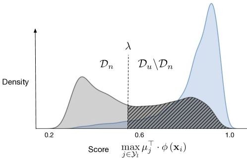
Figure 4: Distribution of OOD score $\max_{j\in\mathcal{Y}_{l}}\boldsymbol{\mu}_{j}^{\top}\cdot\phi(\mathbf{x}_{i})$ for unlabeled data $\mathcal{D}_{u}$ on CIFAR-100. For visual clarity, gray indicates samples from novel classes and blue indicates samples from known classes. The shaded area highlights samples from novel classes but misidentified as known classes.

We next show that using this part of data will be harmful to representation learning. Specifically, we replace $\mathcal{L}_{l}$ to be the following loss:

$$\mathcal{L}_{known}=\sum_{\mathbf{x}\in\tilde{\mathcal{B}}_{k}}\mathcal{L}_{\phi}\left(\mathbf{x};\tau_{k},\mathcal{P}_{k}(\mathbf{x}),\mathcal{N}_{k}(\mathbf{x})\right),$$

where we define $\mathcal{B}_{k}$ to be a minibatch with samples drawn from $\mathcal{D}_{l}\cup(\mathcal{D}_{u}\backslash\mathcal{D}_{n})$—labeled data with known classes, along with the unlabeled data predicted as known classes. And we apply two random augmentations for each sample and generate a multi-viewed batch $\tilde{\mathcal{B}}_{k}$. We denote the embeddings of the multi-viewed batch as $\mathcal{A}_{k}$. The positive set of embeddings is as follows:

$$\mathcal{P}_{k}(\mathbf{x}) =\left\{\mathbf{z}^{\prime}\mid\mathbf{z}^{\prime}\in\left\{\mathcal{A}_{k}\backslash\mathbf{z}\right\},\tilde{y}^{\prime}=\tilde{y}\right\}$$

$$\mathcal{N}_{k}(\mathbf{x}) =\mathcal{A}_{k}\backslash\mathbf{z},$$

where

$$\tilde{y}_{i}=\begin{cases}\hat{y}_{i}\text{ (pseudo-label)}&\text{ if }\mathbf{x}_{i}\in\mathcal{D}_{u}\\ y_{i}\text{ (ground-truth label)},&\text{ if }\mathbf{x}_{i}\in\mathcal{D}_{l}\end{cases}$$

Intuitively, $\mathcal{L}_{known}$ is an extension of $\mathcal{L}_{l}$, where we utilize both labeled and unlabeled data from known classes for representation learning. The final loss now becomes:

$$\mathcal{L}_{\text{Modified}}=\lambda_{n}\mathcal{L}_{n}+\lambda_{k}\mathcal{L}_{known}+\lambda_{u}\mathcal{L}_{u},$$ (10)

We show results in Table 7. Compared to the original loss, the seen accuracy drops by 6.6%. This finding suggests that using $\mathcal{D}_{u}\backslash\mathcal{D}_{n}$ for prototype-based learning is suboptimal.

Table 7: Comparison with loss $\mathcal{L}_{\text{Modified}}$ on CIFAR-100.

Method	CIFAR-100
	All	Novel	Seen
$\mathcal{L}_{\text{Modified}}$	47.7	46.4	62.4
$\mathcal{L}_{\text{OpenCon}}$	53.7	48.7	69.0

Appendix F Proof Details

Proof of Lemma 4.2

Proof.

$$\underset{\phi,\mathbf{M}}{\operatorname{argmax\ }}\sum_{i=1}^{|\mathcal{D}_{n}|}\sum_{c\in\mathcal{Y}_{\text{all}}}q_{i}(c)\log\frac{p\left(\mathbf{x}_{i},c|\phi,\mathbf{M}\right)}{q_{i}(c)} \overset{\mathrm{(a)}}{=}\underset{\phi,\mathbf{M}}{\operatorname{argmax\ }}\sum_{i=1}^{|\mathcal{D}_{n}|}\sum_{c\in\mathcal{Y}_{\text{all}}}q_{i}(c)\log p\left(\mathbf{x}_{i}|c,\phi,\mathbf{M}\right)$$

$$\overset{\mathrm{(b)}}{=}\underset{\phi,\mathbf{M}}{\operatorname{argmax\ }}\sum_{i=1}^{|\mathcal{D}_{n}|}\sum_{c\in\mathcal{Y}_{\text{all}}}\mathbf{1}\{\hat{y}_{i}=c\}\log p\left(\mathbf{x}_{i}|c,\phi,\mathbf{M}\right)$$

$$\overset{\mathrm{(d)}}{=}\underset{\phi,\mathbf{M}}{\operatorname{argmax\ }}\sum_{c\in\mathcal{Y}_{\text{all}}}\sum_{\mathbf{x}\in\mathcal{S}(c)}\log p(\mathbf{x}|c,\phi,\mathbf{M})$$

$$\overset{\mathrm{(e)}}{=}\underset{\phi,\mathbf{M}}{\operatorname{argmax\ }}\sum_{c\in\mathcal{Y}_{\text{all}}}\sum_{\mathbf{x}\in\mathcal{S}(c)}\phi(\mathbf{x})^{\top}\cdot\boldsymbol{\mu}_{c},$$

where equation $(a)$ is given by removing the constant term $q_{i}(c)\log\frac{p(c)}{q_{i}(c)}$ in $\operatorname{argmax}$, (b) is by plugging $q_{i}(c)$, (d) is by reorganizing the index, and (e) is by plugging the vMF density function and removing the constant. ∎

Proof of Lemma 4.3

Proof.

$$\underset{\phi}{\operatorname{argmin\ }}\sum_{\mathbf{x}\in\mathcal{D}_{n}}\mathcal{L}_{a}(\mathbf{x}) =\underset{\phi}{\operatorname{argmin\ }}-\sum_{\mathbf{x}\in\mathcal{D}_{n}}\frac{1}{|\mathcal{P}(\mathbf{x})|}\sum_{\mathbf{z}^{+}\in\mathcal{P}(\mathbf{x})}\phi(\mathbf{x})^{\top}\cdot\mathbf{z}^{+}$$

$$=\underset{\phi}{\operatorname{argmin\ }}-\sum_{c\in\mathcal{Y}_{\text{all}}}\sum_{\mathbf{x}\in\mathcal{S}(c)}\frac{1}{|\mathcal{S}_{c}|-1}\sum_{\boldsymbol{x^{+}}\in\mathcal{S}(c)\backslash\mathbf{x}}\phi(\mathbf{x})^{\top}\cdot\phi(\mathbf{x}^{+})$$

$$=\underset{\phi}{\operatorname{argmin\ }}-\sum_{c\in\mathcal{Y}_{\text{all}}}\sum_{\mathbf{x}\in\mathcal{S}(c)}\frac{1}{|\mathcal{S}_{c}|-1}\left(\left(\sum_{\boldsymbol{x^{+}}\in\mathcal{S}(c)}\phi(\mathbf{x})^{\top}\cdot\phi(\mathbf{x}^{+})\right)-1\right)$$

$$\overset{\mathrm{(a)}}{=}\underset{\phi}{\operatorname{argmin\ }}-\sum_{c\in\mathcal{Y}_{\text{all}}}\sum_{\mathbf{x}\in\mathcal{S}(c)}\eta_{\mathcal{S}_{c}}\phi(\mathbf{x})^{\top}\cdot\boldsymbol{\mu}^{*}_{c}$$

$$\overset{\mathrm{(b)}}{\approx}\underset{\phi}{\operatorname{argmax\ }}\sum_{c\in\mathcal{Y}_{\text{all}}}\sum_{\mathbf{x}\in\mathcal{S}(c)}\phi(\mathbf{x})^{\top}\cdot\boldsymbol{\mu}^{*}_{c},$$

where in (a) $\eta_{\mathcal{S}_{c}}=\frac{|\mathcal{S}_{c}|}{|\mathcal{S}_{c}|-1}\|\mathbb{E}_{\mathbf{x}\in\mathcal{S}(c)}[\phi(\mathbf{x})]\|_{2}$ is a constant value close to 1, and in (b) we show the approximation to the optimization target in Equation 8 with the fixed prototypes. The proof is done by using the equation in Lemma 4.2. ∎

Appendix G Results on CIFAR-10

We show results for CIFAR-10 in Table 8, where OpenCon consistently outperforms strong baselines, particularly ORCA and GCD. Classes are divided into 50% known and 50% novel classes. We then select 50% of known classes as the labeled dataset and the rest as the unlabeled set. The division is consistent with (Cao et al., 2022), which allows us to compare the performance in a fair setting.

Table 8: Results on CIFAR-10. Asterisk (^⋆) denotes that the original method can not recognize seen classes. Dagger (^†) denotes the original method can not detect novel classes (and we had to extend it). Results on GCD, ORCA, and OpenCon (mean and standard deviation) are averaged over five different runs. The ORCA results are reported by running the official repo (Cao et al., ).

Method	CIFAR-10
	All	Novel	Seen
†FixMatch (Kurakin et al., 2020)	49.5	50.4	71.5
†DS3L (Guo et al., 2020)	40.2	45.3	77.6
†CGDL (Sun et al., 2020)	39.7	44.6	72.3
⋆DTC (Han et al., 2019)	38.3	39.5	53.9
⋆RankStats (Zhao & Han, 2021)	82.9	81.0	86.6
⋆SimCLR (Chen et al., 2020a)	51.7	63.4	58.3
ORCA (Cao et al., 2022)	88.3±0.3	87.5±0.2	89.9±0.4
GCD (Vaze et al., 2022)	87.5±0.5	86.7±0.4	90.1±0.3
OpenCon (Ours)	90.4±0.6	91.1±0.1	89.3±0.2

Appendix H More Qualitative Comparisons of Embeddings

In Figure 5, we visualize the feature embeddings for a subset of 20 classes using UMAP (McInnes et al., 2018). This covers more classes than what has been shown in the main paper (Figure 2). The model is trained on ImageNet-100. OpenCon produces a more compact and distinguishable embedding space than GCD and ORCA.

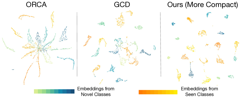
Figure 5: UMAP (McInnes et al., 2018) visualization of the feature embedding from 20 classes (10 for seen, 10 for novel). The model is trained on ImageNet-100 with ORCA (Cao et al., 2022), GCD (Vaze et al., 2022), and OpenCon (ours).

Appendix I Hyperparameters and Sensitivity Analysis

In this section, we introduce the hyper-parameter settings for OpenCon. We also show a validation strategy to determine important hyper-parameters (weight and temperature) in loss $\mathcal{L}_{OpenCon}$ and conduct a sensitivity analysis to show that the validation strategy can select near-optimal hyper-parameters. We start by introducing the basic training setting.

For CIFAR-100/ImageNet-100, the model is trained for 200/120 epochs with batch-size 512 using stochastic gradient descent with momentum 0.9, and weight decay $10^{-4}$. The learning rate starts at 0.02 and decays by a factor of 10 at the 50% and the 75% training stage. The momentum for prototype updating $\gamma$ is fixed at 0.9. The percentile $p$ for OOD detection is 70%. We fix the weight for the KL-divergence regularizer to be 0.05.

Since the label for $\mathcal{D}_{u}$ is not available, we propose a validation strategy by using labeled data $\mathcal{D}_{l}$. Specifically, we split the classes in $\mathcal{Y}_{l}$ equally into two parts: known classes and “novel” classes (for which we know the labels). Moreover, $50\%$ samples of the selected known classes are labeled. We further use the new validation dataset to select the best hyper-parameters by grid searching. The selected hyper-parameter groups are summarized in Table 9. Note that the only difference between CIFAR-100 and ImageNet-100 settings is the temperature of the self-supervised loss $\mathcal{L}_{u}$.

We show the sensitivity of hyper-parameters in Figure 6. The performance comparison in the bar plot for each hyper-parameter is reported by fixing other hyper-parameters. We see that our validation strategy successfully selects $\lambda_{l}$, $\lambda_{u}$, and $\tau_{l}$ with the optimal one, and the other three $\lambda_{n}$, $\tau_{u}$ and $\tau_{n}$ are close to the optimal (with <1% gap in overall accuracy).

Table 9: Hyperparameters in OpenCon.

	$\lambda_{n}$	$\tau_{n}$	$\lambda_{l}$	$\tau_{l}$	$\lambda_{u}$	$\tau_{u}$
ImageNet-100	0.1	0.7	0.2	0.1	1	0.6
CIFAR-100	0.1	0.7	0.2	0.1	1	0.4

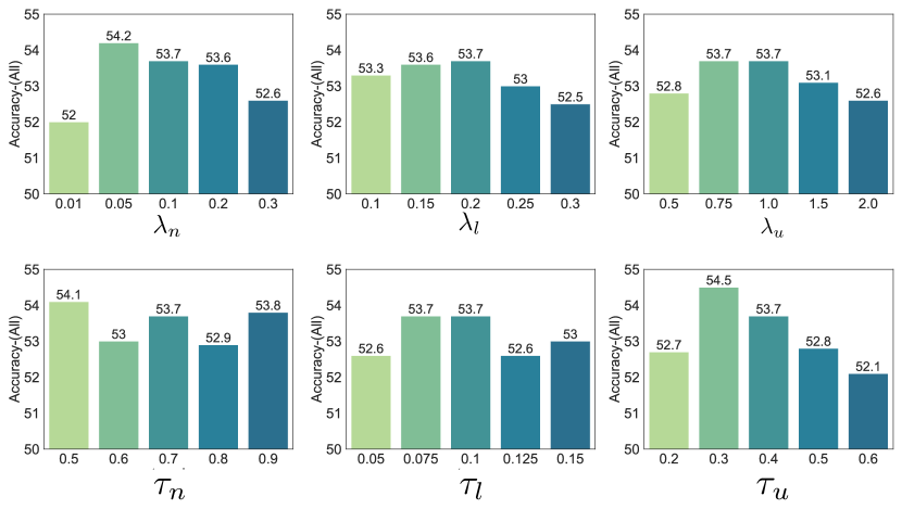
Figure 6: Sensitivity analysis of hyper-parameters on CIFAR-100. The overall accuracy is reported on three (weight, temperature) pairs: ($\lambda_{n}$, $\tau_{n}$) for loss $\mathcal{L}_{n}$, ($\lambda_{l}$, $\tau_{l}$) for loss $\mathcal{L}_{l}$, and the ($\lambda_{u}$, $\tau_{u}$) for loss $\mathcal{L}_{u}$. The middle bar in each plot corresponds to the hyperparameter value used in our main experiments.

Appendix J OOD Detection Comparison

We compare different OOD detection methods in Table 10. Results show that several popular OOD detection methods produce similar OOD detection performance. Note that Mahalanobis (Lee et al., 2018) require heavier computation which causes an unbearable burden in the training stage. Our method incurs minimal computational overhead.

Table 10: Comparison of OOD detection performance with popular methods. Results are reported on CIFAR-100. Samples from 50 known classes are treated as in-distribution (ID) data and samples from the remaining 50 classes are used as out-of-distribution (OOD) data. The OOD detection threshold is estimated on the labeled known classes $\mathcal{D}_{l}$.

Method	FPR95	AUROC
MSP (Hendrycks & Gimpel, 2017)	58.9	86.0
Energy (Liu et al., 2020)	57.1	87.4
Mahalanobis (Lee et al., 2018)	54.6	88.7
Ours	57.1	87.4

Appendix K Sensitivity Analysis on Estimated Class Number

In this section, we provide the sensitivity analysis of the estimated class number on CIFAR-100. We noticed that when the estimated class number is much larger than the actual class number (100), some prototypes will never be predicted by any of the training samples. So the training process will converge to solutions that closely match the ground truth number of classes. We show in Table 11 comparing the initial class number and the class number after converging. It shows that an overestimation of the class number has a negligible effect on the final converged class number.

Table 11: Converged class numbers under different initial class numbers.

Initial Class Number	100	110	120	130	150	200
Converged Class Number	100	106	108	109	109	109

Appendix L Performance on ImageNet-1k

To verify the effectiveness of OpenCon in a large-scale setting, we provide the results on ImageNet-1k in Table 12. The experiments are based on 500 known classes and 500 novel classes, with a labeling ratio = 0.5 for known classes. We notice that ORCA’s performance degrades significantly in a large-scale setting. OpenCon significantly outperforms the best baseline GCD by 8.8%, in terms of overall accuracy.

Table 12: Comparison of classification accuracy on ImageNet-1k.

Method	ImageNet-1k
	All	Novel	Seen
ORCA	17.6	20.5	35.3
GCD	35.8	36.9	69.0
OpenCon (ours)	44.6	42.5	73.9

Appendix M Differences w.r.t. Prototypical Contrastive Learning

Our work is inspired by yet differs substantially from unsupervised prototypical contrastive learning (PCL) (Li et al., 2021b), in terms of problem setup (Section 2), learning objective (Section 3), and theoretical insights (Section 4). Importantly, PCL relies entirely on the unlabeled data $\mathcal{D}_{u}$ and does not leverage the availability of the labeled dataset. Instead, we consider the open-world semi-supervised learning setting (Cao et al., 2022), and leverage both labeled data (from known classes) and unlabeled data (from both known and novel classes). This setting leads to unique challenges that were not considered in PCL, such as how to learn strong representations for both the known and novel classes in a unified framework; and how to perform OOD detection to separate known and novel samples in the unlabeled data. OpenCon makes new contributions by addressing these challenges in an end-to-end trainable framework, supported by theoretical analysis.

In Table 13, we show evidence that the PCL does not trivially apply in this open-world setting, and under-performs OpenCon.

Table 13: Comparison with PCL.

Method	CIFAR-100
	All	Novel	Seen
PCL (Li et al., 2021b)	42.1	44.5	39.0
OpenCon (Ours)	53.7	48.7	69.0

Appendix N Experiments on Fine-grained Datasets

The fine-grained task is more challenging since the known and novel classes can be similar. We provide the results of the fine-grained task on Stanford Cars (Krause et al., 2013), CUB-200 (Vaze et al., 2021) and Herbarium19 (Tan et al., 2019) in Table 14. We adopt the ViT-B/16 architecture with DINO pre-trained weights  (Caron et al., 2021). Results show that OpenCon outperforms the best baseline GCD by 10.1% on the Stanford Cars dataset, in terms of overall accuracy.

Table 14: Comparison on fine-grained datasets.

Method	CUB-200			Stanford Cars			Herbarium19
	All	Novel	Seen	All	Novel	Seen	All	Novel	Seen
$k$-Means (MacQueen, 1967)	34.3	32.1	38.9	13.8	10.6	12.8	12.9	12.8	12.9
RankStats+ (Zhao & Han, 2021)	33.3	24.2	51.6	28.3	12.1	61.8	27.9	12.8	55.8
UNO+ (Fini et al., 2021)	35.1	28.1	49.0	35.5	18.6	70.5	28.3	14.7	53.7
GCD (Vaze et al., 2022)	51.3	48.7	56.6	39.0	29.9	57.6	35.4	27.0	51.0
OpenCon (Ours)	54.7	52.1	63.8	49.1	32.7	78.6	39.3	28.6	58.9

Appendix O Hardware and Software

We run all experiments with Python 3.7 and PyTorch 1.7.1, using NVIDIA GeForce RTX 2080Ti GPUs.

References

- Bendale & Boult (2016) Abhijit Bendale and Terrance E Boult. Towards open set deep networks. In Proceedings of the IEEE conference on computer vision and pattern recognition, pp. 1563–1572, 2016.
- (2) Kaidi Cao, Maria Brbic, and Jure Leskovec. Open-world semi-supervised learning. URL https://github.com/snap-stanford/orca.
- Cao et al. (2022) Kaidi Cao, Maria Brbic, and Jure Leskovec. Open-world semi-supervised learning. In Proceedings of the International Conference on Learning Representations, 2022.
- Caron et al. (2020) Mathilde Caron, Ishan Misra, Julien Mairal, Priya Goyal, Piotr Bojanowski, and Armand Joulin. Unsupervised learning of visual features by contrasting cluster assignments. Proceedings of Advances in Neural Information Processing Systems, 2020.
- Caron et al. (2021) Mathilde Caron, Hugo Touvron, Ishan Misra, Hervé Jégou, Julien Mairal, Piotr Bojanowski, and Armand Joulin. Emerging properties in self-supervised vision transformers. In Proceedings of the International Conference on Computer Vision (ICCV), 2021.
- Cha et al. (2021) Hyuntak Cha, Jaeho Lee, and Jinwoo Shin. Co2l: Contrastive continual learning. In Proceedings of the IEEE/CVF International Conference on Computer Vision, pp. 9516–9525, 2021.
- Chapelle et al. (2006) Olivier Chapelle, Bernhard Schölkopf, and Alexander Zien (eds.). Semi-Supervised Learning. The MIT Press, 2006.
- Chen et al. (2020a) Ting Chen, Simon Kornblith, Mohammad Norouzi, and Geoffrey Hinton. A simple framework for contrastive learning of visual representations. In Proceedings of the international conference on machine learning, pp. 1597–1607. PMLR, 2020a.
- Chen et al. (2020b) Ting Chen, Simon Kornblith, Kevin Swersky, Mohammad Norouzi, and Geoffrey E Hinton. Big self-supervised models are strong semi-supervised learners. Proceedings of Advances in Neural Information Processing Systems, 33:22243–22255, 2020b.
- Chen et al. (2020c) Yanbei Chen, Xiatian Zhu, Wei Li, and Shaogang Gong. Semi-supervised learning under class distribution mismatch. In Proceedings of the AAAI Conference on Artificial Intelligence, volume 34, pp. 3569–3576, 2020c.
- Cui et al. (2021) Jiequan Cui, Zhisheng Zhong, Shu Liu, Bei Yu, and Jiaya Jia. Parametric contrastive learning. In Proceedings of the IEEE/CVF International Conference on Computer Vision, pp. 715–724, 2021.
- Deng et al. (2009) Jia Deng, Wei Dong, Richard Socher, Li-Jia Li, Kai Li, and Li Fei-Fei. Imagenet: A large-scale hierarchical image database. In Proceedings of the IEEE Conference on Computer Vision and Pattern Recognition, pp. 248–255, 2009.
- Dosovitskiy et al. (2020) Alexey Dosovitskiy, Lucas Beyer, Alexander Kolesnikov, Dirk Weissenborn, Xiaohua Zhai, Thomas Unterthiner, Mostafa Dehghani, Matthias Minderer, Georg Heigold, Sylvain Gelly, et al. An image is worth 16x16 words: Transformers for image recognition at scale. In International Conference on Learning Representations, 2020.
- Dwibedi et al. (2021) Debidatta Dwibedi, Yusuf Aytar, Jonathan Tompson, Pierre Sermanet, and Andrew Zisserman. With a little help from my friends: Nearest-neighbor contrastive learning of visual representations. In Proceedings of the IEEE/CVF International Conference on Computer Vision, pp. 9588–9597, 2021.
- Fini et al. (2021) Enrico Fini, Enver Sangineto, Stéphane Lathuilière, Zhun Zhong, Moin Nabi, and Elisa Ricci. A unified objective for novel class discovery. In Proceedings of the IEEE/CVF International Conference on Computer Vision, pp. 9284–9292, 2021.
- Fisher (1953) Ronald Aylmer Fisher. Dispersion on a sphere. Proceedings of the Royal Society of London. Series A. Mathematical and Physical Sciences, 217(1130):295–305, 1953.
- Fumera & Roli (2002) Giorgio Fumera and Fabio Roli. Support vector machines with embedded reject option. In International Workshop on Support Vector Machines, pp. 68–82. Springer, 2002.
- Gal & Ghahramani (2016) Yarin Gal and Zoubin Ghahramani. Dropout as a bayesian approximation: Representing model uncertainty in deep learning. In Proceedings of the International Conference on Machine Learning, pp. 1050–1059, 2016.
- Gao et al. (2021) Yizhao Gao, Nanyi Fei, Guangzhen Liu, Zhiwu Lu, and Tao Xiang. Contrastive prototype learning with augmented embeddings for few-shot learning. In Proceedings of the Thirty-Seventh Conference on Uncertainty in Artificial Intelligence, pp. 140–150, 2021.
- Goyal et al. (2021) Priya Goyal, Mathilde Caron, Benjamin Lefaudeux, Min Xu, Pengchao Wang, Vivek Pai, Mannat Singh, Vitaliy Liptchinsky, Ishan Misra, Armand Joulin, et al. Self-supervised pretraining of visual features in the wild. arXiv preprint arXiv:2103.01988, 2021.
- Guo et al. (2020) Lan-Zhe Guo, Zhen-Yu Zhang, Yuan Jiang, Yu-Feng Li, and Zhi-Hua Zhou. Safe deep semi-supervised learning for unseen-class unlabeled data. In Proceedings of the international conference on machine learning, volume 119 of Proceedings of Machine Learning Research, pp. 3897–3906. PMLR, 13–18 Jul 2020.
- Han et al. (2019) Kai Han, Andrea Vedaldi, and Andrew Zisserman. Learning to discover novel visual categories via deep transfer clustering. In Proceedings of the IEEE/CVF International Conference on Computer Vision, 2019.
- He et al. (2020) Kaiming He, Haoqi Fan, Yuxin Wu, Saining Xie, and Ross Girshick. Momentum contrast for unsupervised visual representation learning. In Proceedings of the IEEE Conference on Computer Vision and Pattern Recognition, pp. 9729–9738, 2020.
- Hendrycks & Gimpel (2017) Dan Hendrycks and Kevin Gimpel. A baseline for detecting misclassified and out-of-distribution examples in neural networks. Proceedings of International Conference on Learning Representations, 2017.
- Hsu et al. (2018) Yen-Chang Hsu, Zhaoyang Lv, and Zsolt Kira. Learning to cluster in order to transfer across domains and tasks. Proceedings of the International Conference on Learning Representations, 2018.
- Hsu et al. (2019) Yen-Chang Hsu, Zhaoyang Lv, Joel Schlosser, Phillip Odom, and Zsolt Kira. Multi-class classification without multi-class labels. Proceedings of the International Conference on Learning Representations, 2019.
- Huang et al. (2021a) Junkai Huang, Chaowei Fang, Weikai Chen, Zhenhua Chai, Xiaolin Wei, Pengxu Wei, Liang Lin, and Guanbin Li. Trash to treasure: Harvesting ood data with cross-modal matching for open-set semi-supervised learning. In Proceedings of the IEEE/CVF International Conference on Computer Vision, pp. 8310–8319, 2021a.
- Huang & Li (2021) Rui Huang and Yixuan Li. Towards scaling out-of-distribution detection for large semantic space. In Proceedings of the IEEE/CVF Conference on Computer Vision and Pattern Recognition, 2021.
- Huang et al. (2021b) Rui Huang, Andrew Geng, and Yixuan Li. On the importance of gradients for detecting distributional shifts in the wild. In Proceedings of the Advances in Neural Information Processing Systems, 2021b.
- Jiang et al. (2021) Ziyu Jiang, Tianlong Chen, Ting Chen, and Zhangyang Wang. Improving contrastive learning on imbalanced data via open-world sampling. Proceedings of Advances in Neural Information Processing Systems, 34, 2021.
- Karim et al. (2022) Nazmul Karim, Mamshad Nayeem Rizve, Nazanin Rahnavard, Ajmal Mian, and Mubarak Shah. Unicon: Combating label noise through uniform selection and contrastive learning. In Proceedings of the IEEE Conference on Computer Vision and Pattern Recognition, 2022.
- Khosla et al. (2020) Prannay Khosla, Piotr Teterwak, Chen Wang, Aaron Sarna, Yonglong Tian, Phillip Isola, Aaron Maschinot, Ce Liu, and Dilip Krishnan. Supervised contrastive learning. Proceedings of Advances in Neural Information Processing Systems, 33:18661–18673, 2020.
- Krause et al. (2013) Jonathan Krause, Michael Stark, Jia Deng, and Li Fei-Fei. 3d object representations for fine-grained categorization. In Proceedings of the IEEE international conference on computer vision workshops, pp. 554–561, 2013.
- Krizhevsky et al. (2009) Alex Krizhevsky, Geoffrey Hinton, et al. Learning multiple layers of features from tiny images. 2009.
- Kuhn & Yaw (1955) H. W. Kuhn and Bryn Yaw. The hungarian method for the assignment problem. Naval Res. Logist. Quart, pp. 83–97, 1955.
- Kurakin et al. (2020) Alex Kurakin, Chun-Liang Li, Colin Raffel, David Berthelot, Ekin Dogus Cubuk, Han Zhang, Kihyuk Sohn, Nicholas Carlini, and Zizhao Zhang. Fixmatch: Simplifying semi-supervised learning with consistency and confidence. In Proceedings of Advances in Neural Information Processing Systems, 2020.
- Laine & Aila (2017) Samuli Laine and Timo Aila. Temporal ensembling for semi-supervised learning. Proceedings of the International Conference on Learning Representations, 2017.
- Lakshminarayanan et al. (2017) Balaji Lakshminarayanan, Alexander Pritzel, and Charles Blundell. Simple and scalable predictive uncertainty estimation using deep ensembles. In Proceedings of Advances in Neural Information Processing Systems, pp. 6402–6413, 2017.
- Lee et al. (2013) Dong-Hyun Lee et al. Pseudo-label: The simple and efficient semi-supervised learning method for deep neural networks. In Workshop on challenges in representation learning, ICML, volume 3, pp. 896, 2013.
- Lee et al. (2018) Kimin Lee, Kibok Lee, Honglak Lee, and Jinwoo Shin. A simple unified framework for detecting out-of-distribution samples and adversarial attacks. In Proceedings of Advances in Neural Information Processing Systems, pp. 7167–7177, 2018.
- Li et al. (2020) Junnan Li, Caiming Xiong, and Steven Hoi. Mopro: Webly supervised learning with momentum prototypes. In International Conference on Learning Representations, 2020.
- Li et al. (2021a) Junnan Li, Caiming Xiong, and Steven C.H. Hoi. Semi-supervised learning with contrastive graph regularization. In Proceedings of the International Conference on Learning Representations, 2021a.
- Li et al. (2021b) Junnan Li, Pan Zhou, Caiming Xiong, and Steven CH Hoi. Prototypical contrastive learning of unsupervised representations. Proceedings of the International Conference on Learning Representations, 2021b.
- Li et al. (2022a) Shikun Li, Xiaobo Xia, Shiming Ge, and Tongliang Liu. Selective-supervised contrastive learning with noisy labels. In Proceedings of the IEEE Conference on Computer Vision and Pattern Recognition, 2022a.
- Li et al. (2022b) Tianhong Li, Peng Cao, Yuan Yuan, Lijie Fan, Yuzhe Yang, Rogério Feris, Piotr Indyk, and Dina Katabi. Targeted supervised contrastive learning for long-tailed recognition. In Proceedings of the IEEE Conference on Computer Vision and Pattern Recognition, 2022b.
- Liang et al. (2018) Shiyu Liang, Yixuan Li, and Rayadurgam Srikant. Enhancing the reliability of out-of-distribution image detection in neural networks. In Proceedings of the International Conference on Learning Representations, 2018.
- Lin et al. (2021) Ziqian Lin, Sreya Dutta Roy, and Yixuan Li. Mood: Multi-level out-of-distribution detection. In Proceedings of the IEEE/CVF Conference on Computer Vision and Pattern Recognition, pp. 15313–15323, June 2021.
- Liu et al. (2020) Weitang Liu, Xiaoyun Wang, John Owens, and Yixuan Li. Energy-based out-of-distribution detection. Proceedings of Advances in Neural Information Processing Systems, 33:21464–21475, 2020.
- MacQueen (1967) J MacQueen. Classification and analysis of multivariate observations. In 5th Berkeley Symp. Math. Statist. Probability, pp. 281–297, 1967.
- Maddox et al. (2019) Wesley J Maddox, Pavel Izmailov, Timur Garipov, Dmitry P Vetrov, and Andrew Gordon Wilson. A simple baseline for bayesian uncertainty in deep learning. Advances in Neural Information Processing Systems, 32:13153–13164, 2019.
- Malinin & Gales (2018) Andrey Malinin and Mark Gales. Predictive uncertainty estimation via prior networks. In Advances in Neural Information Processing Systems, pp. 7047–7058, 2018.
- Malinin & Gales (2019) Andrey Malinin and Mark Gales. Reverse kl-divergence training of prior networks: Improved uncertainty and adversarial robustness. In Advances in Neural Information Processing Systems, 2019.
- McInnes et al. (2018) Leland McInnes, John Healy, Nathaniel Saul, and Lukas Grossberger. Umap: Uniform manifold approximation and projection. The Journal of Open Source Software, 3(29):861, 2018.
- Ming et al. (2022a) Yifei Ming, Ziyang Cai, Jiuxiang Gu, Yiyou Sun, Wei Li, and Yixuan Li. Delving into out-of-distribution detection with vision-language representations. Advances in neural information processing systems, 2022a.
- Ming et al. (2022b) Yifei Ming, Yiyou Sun, Ousmane Dia, and Yixuan Li. Cider: Exploiting hyperspherical embeddings for out-of-distribution detection. arXiv preprint arXiv:2203.04450, 2022b.
- Morteza & Li (2022) Peyman Morteza and Yixuan Li. Provable guarantees for understanding out-of-distribution detection. Proceedings of the AAAI Conference on Artificial Intelligence, 2022.
- Oliver et al. (2018) Avital Oliver, Augustus Odena, Colin A Raffel, Ekin Dogus Cubuk, and Ian Goodfellow. Realistic evaluation of deep semi-supervised learning algorithms. Proceedings of Advances in Neural Information Processing Systems, 31, 2018.
- Park et al. (2021) Jongjin Park, Sukmin Yun, Jongheon Jeong, and Jinwoo Shin. Opencos: Contrastive semi-supervised learning for handling open-set unlabeled data. arXiv preprint arXiv:2107.08943, 2021.
- Rebuffi et al. (2020) Sylvestre-Alvise Rebuffi, Sebastien Ehrhardt, Kai Han, Andrea Vedaldi, and Andrew Zisserman. Semi-supervised learning with scarce annotations. In Proceedings of the IEEE/CVF Conference on Computer Vision and Pattern Recognition Workshops, pp. 762–763, 2020.
- Rizve et al. (2022) Mamshad Nayeem Rizve, Navid Kardan, Salman Khan, Fahad Shahbaz Khan, and Mubarak Shah. Openldn: Learning to discover novel classes for open-world semi-supervised learning. Proceedings of the European Conference on Computer Vision, 2022.
- Saito et al. (2021) Kuniaki Saito, Donghyun Kim, and Kate Saenko. Openmatch: Open-set consistency regularization for semi-supervised learning with outliers. Proceedings of Advances in Neural Information Processing Systems, 2021.
- Sajjadi et al. (2016) Mehdi Sajjadi, Mehran Javanmardi, and Tolga Tasdizen. Regularization with stochastic transformations and perturbations for deep semi-supervised learning. Proceedings of Advances in Neural Information Processing Systems, 29, 2016.
- Sehwag et al. (2021) Vikash Sehwag, Mung Chiang, and Prateek Mittal. Ssd: A unified framework for self-supervised outlier detection. In International Conference on Learning Representations, 2021.
- Sun et al. (2020) Xin Sun, Zhenning Yang, Chi Zhang, Keck-Voon Ling, and Guohao Peng. Conditional gaussian distribution learning for open set recognition. In Proceedings of the IEEE Conference on Computer Vision and Pattern Recognition, pp. 13480–13489, 2020.
- Sun & Li (2022) Yiyou Sun and Yixuan Li. Dice: Leveraging sparsification for out-of-distribution detection. In European Conference on Computer Vision, 2022.
- Sun et al. (2017) Yiyou Sun, Tonghua Su, and Zhiying Tu. Faster r-cnn based autonomous navigation for vehicles in warehouse. In 2017 IEEE International Conference on Advanced Intelligent Mechatronics (AIM), pp. 1639–1644. IEEE, 2017.
- Sun et al. (2021) Yiyou Sun, Chuan Guo, and Yixuan Li. React: Out-of-distribution detection with rectified activations. In Advances in Neural Information Processing Systems, 2021.
- Sun et al. (2022) Yiyou Sun, Yifei Ming, Xiaojin Zhu, and Yixuan Li. Out-of-distribution detection with deep nearest neighbors. In Proceedings of the International Conference on Machine Learning, 2022.
- Tack et al. (2020) Jihoon Tack, Sangwoo Mo, Jongheon Jeong, and Jinwoo Shin. Csi: Novelty detection via contrastive learning on distributionally shifted instances. In Advances in Neural Information Processing Systems, 2020.
- Tan et al. (2019) Kiat Chuan Tan, Yulong Liu, Barbara Ambrose, Melissa Tulig, and Serge Belongie. The herbarium challenge 2019 dataset. arXiv preprint arXiv:1906.05372, 2019.
- Tian et al. (2021) Yonglong Tian, Olivier J Henaff, and Aäron van den Oord. Divide and contrast: Self-supervised learning from uncurated data. In Proceedings of the IEEE/CVF International Conference on Computer Vision, pp. 10063–10074, 2021.
- Tsai et al. (2022) Yao-Hung Hubert Tsai, Tianqin Li, Weixin Liu, Peiyuan Liao, Ruslan Salakhutdinov, and Louis-Philippe Morency. Learning weakly-supervised contrastive representations. In International Conference on Learning Representations, 2022.
- Van den Oord et al. (2018) Aaron Van den Oord, Yazhe Li, and Oriol Vinyals. Representation learning with contrastive predictive coding. arXiv e-prints, pp. arXiv–1807, 2018.
- Vaze et al. (2021) Sagar Vaze, Kai Han, Andrea Vedaldi, and Andrew Zisserman. Open-set recognition: A good closed-set classifier is all you need. Proceedings of the International Conference on Learning Representations, 2021.
- Vaze et al. (2022) Sagar Vaze, Kai Han, Andrea Vedaldi, and Andrew Zisserman. Generalized category discovery. In Proceedings of the IEEE Conference on Computer Vision and Pattern Recognition, 2022.
- Wang et al. (2022) Haobo Wang, Ruixuan Xiao, Yixuan Li, Lei Feng, Gang Niu, Gang Chen, and Junbo Zhao. Pico: Contrastive label disambiguation for partial label learning. Proceedings of the International Conference on Learning Representations, 2022.
- Wang et al. (2021) Haoran Wang, Weitang Liu, Alex Bocchieri, and Yixuan Li. Can multi-label classification networks know what they don’t know? Proceedings of the Advances in Neural Information Processing Systems, 2021.
- Wang & Isola (2020) Tongzhou Wang and Phillip Isola. Understanding contrastive representation learning through alignment and uniformity on the hypersphere. In Proceedings of the International Conference on Machine Learning, pp. 9929–9939. PMLR, 2020.
- Wu et al. (2021) Zhi-Fan Wu, Tong Wei, Jianwen Jiang, Chaojie Mao, Mingqian Tang, and Yu-Feng Li. Ngc: A unified framework for learning with open-world noisy data. In Proceedings of the IEEE/CVF International Conference on Computer Vision, pp. 62–71, 2021.
- Yang et al. (2022a) Fan Yang, Kai Wu, Shuyi Zhang, Guannan Jiang, Yong Liu, Feng Zheng, Wei Zhang, Chengjie Wang, and Long Zeng. Class-aware contrastive semi-supervised learning. In Proceedings of the IEEE Conference on Computer Vision and Pattern Recognition, 2022a.
- Yang et al. (2022b) Jingkang Yang, Pengyun Wang, Dejian Zou, Zitang Zhou, Kunyuan Ding, Wenxuan Peng, Haoqi Wang, Guangyao Chen, Bo Li, Yiyou Sun, et al. Openood: Benchmarking generalized out-of-distribution detection. arXiv preprint arXiv:2210.07242, 2022b.
- Yu et al. (2020) Qing Yu, Daiki Ikami, Go Irie, and Kiyoharu Aizawa. Multi-task curriculum framework for open-set semi-supervised learning. In Proceedings of the European Conference on Computer Vision, pp. 438–454. Springer, 2020.
- Zha et al. (2001) Hongyuan Zha, Xiaofeng He, Chris Ding, Ming Gu, and Horst Simon. Spectral relaxation for k-means clustering. Advances in neural information processing systems, 14, 2001.
- Zhai et al. (2019) Xiaohua Zhai, Avital Oliver, Alexander Kolesnikov, and Lucas Beyer. S4l: Self-supervised semi-supervised learning. In Proceedings of the IEEE/CVF International Conference on Computer Vision, pp. 1476–1485, 2019.
- Zhang et al. (2021) Dejiao Zhang, Feng Nan, Xiaokai Wei, Shangwen Li, Henghui Zhu, Kathleen McKeown, Ramesh Nallapati, Andrew Arnold, and Bing Xiang. Supporting clustering with contrastive learning. Proceedings of the North American Chapter of the Association for Computational Linguistics, 2021.
- Zhang et al. (2022a) Shu Zhang, Ran Xu, Caiming Xiong, and Chetan Ramaiah. Use all the labels: A hierarchical multi-label contrastive learning framework. In Proceedings of the IEEE Conference on Computer Vision and Pattern Recognition, 2022a.
- Zhang et al. (2022b) Yuhang Zhang, Xiaopeng Zhang, Jie Li, Robert Qiu, Haohang Xu, and Qi Tian. Semi-supervised contrastive learning with similarity co-calibration. IEEE Transactions on Multimedia, 2022b.
- Zhao & Han (2021) Bingchen Zhao and Kai Han. Novel visual category discovery with dual ranking statistics and mutual knowledge distillation. Proceedings of Advances in Neural Information Processing Systems, 34, 2021.
- Zheng et al. (2021) Mingkai Zheng, Fei Wang, Shan You, Chen Qian, Changshui Zhang, Xiaogang Wang, and Chang Xu. Weakly supervised contrastive learning. Proceedings of the IEEE/CVF International Conference on Computer Vision, 2021.
- Zhong et al. (2021a) Zhun Zhong, Enrico Fini, Subhankar Roy, Zhiming Luo, Elisa Ricci, and Nicu Sebe. Neighborhood contrastive learning for novel class discovery. In Proceedings of the IEEE Conference on Computer Vision and Pattern Recognition, pp. 10867–10875, 2021a.
- Zhong et al. (2021b) Zhun Zhong, Linchao Zhu, Zhiming Luo, Shaozi Li, Yi Yang, and Nicu Sebe. Openmix: Reviving known knowledge for discovering novel visual categories in an open world. In Proceedings of the IEEE Conference on Computer Vision and Pattern Recognition, pp. 9462–9470, 2021b.