Globally Consistent Video Depth and Pose Estimation with Efficient Test-Time Training

Abstract

Dense depth and pose estimation is a vital prerequisite for various video applications. Traditional solutions suffer from the robustness of sparse feature tracking and insufficient camera baselines in videos. Therefore, recent methods utilize learning-based optical flow and depth prior to estimate dense depth. However, previous works require heavy computation time or yield sub-optimal depth results. We present GCVD, a globally consistent method for learning-based video structure from motion (SfM) in this paper. GCVD integrates a compact pose graph into the CNN-based optimization to achieve globally consistent estimation from an effective keyframe selection mechanism. It can improve the robustness of learning-based methods with flow-guided keyframes and well-established depth prior. Experimental results show that GCVD outperforms the state-of-the-art methods on both depth and pose estimation. Besides, the runtime experiments reveal that it provides strong efficiency in both short- and long-term videos with global consistency provided.

Introduction

Acquiring dense depth and camera pose from videos is essential for various applications including augmented reality (Holynski and Kopf 2018; Du et al. 2020), video frame interpolation (Bao et al. 2019), view synthesis (Choi et al. 2019; Yoon et al. 2020; Liu et al. 2021) and stabilization (Liu et al. 2009; Lee et al. 2021). In this paper, we propose a learning-based approach to achieve the concurrent inference of scene depth and camera pose from offline videos. Our study belongs to the research track of SfM with the videos acquired. Unlike visual SLAM (Engel, Schöps, and Cremers 2014; Mur-Artal, Montiel, and Tardos 2015; et al. 2017; Teed and Deng 2021) assuming streaming videos that should be estimated on-line, more information of batched frames stored in the video can be used for a globally consistency estimation.

Inferring both depths and poses for every frame is essentially a challenging chicken-and-egg problem. Traditional solutions rely on the established SfM tools (e.g., COLMAP (Schonberger and Frahm 2016)) to estimate the camera trajectory and then perform multi-view stereo. However, the tools often yield incomplete depth and suffer from the robustness issue due to the fragile, sparse feature tracking. Especially in the videos containing dynamic objects, motion blur, or large texture-less regions, the estimation process usually fail early even in the pre-processing step.

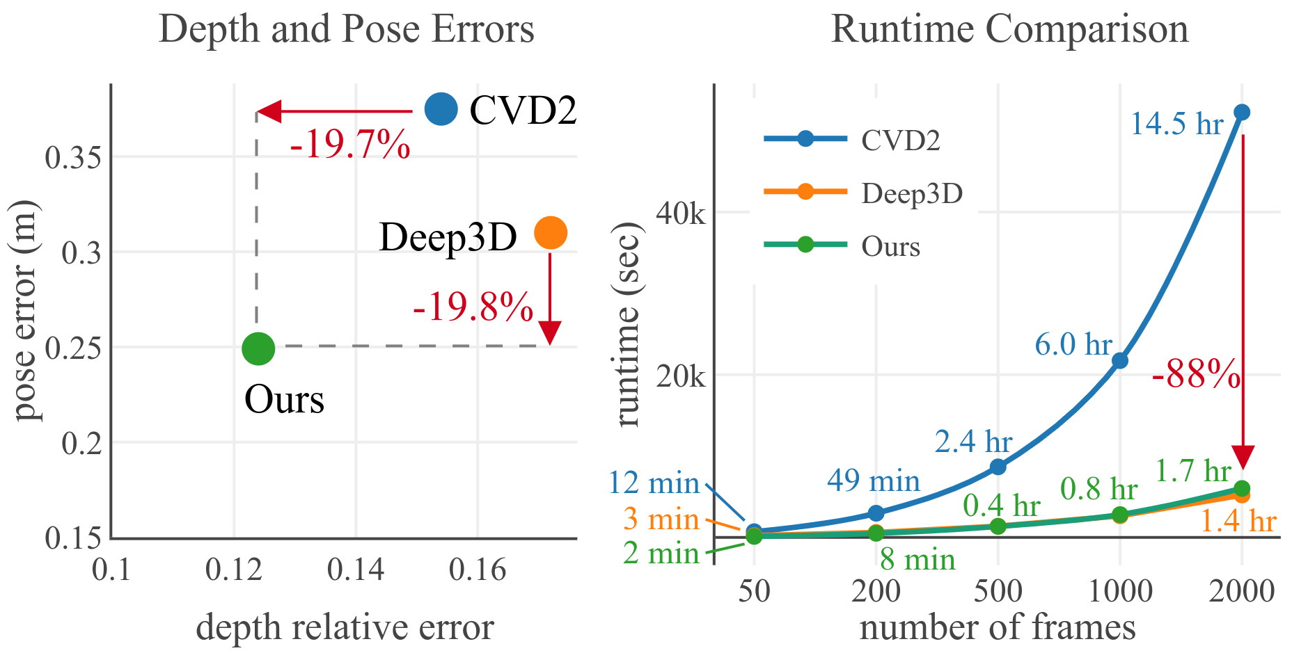
Figure 1: Comparison of estimation errors and runtime. The proposed method outperforms the state-of-the-art methods CVD2 (Kopf, Rong, and Huang 2021) and Deep3D (Lee et al. 2021) on both depth and pose estimation on 7-Scenes dataset (Shotton et al. 2013). Furthermore, our method performs the fastest in short videos; and slightly slower than Deep3D in long videos while Deep3D does not maintain global consistency.

In learning-based studies, many works (Eigen, Puhrsch, and Fergus 2014; Ranftl et al. 2020; Miangoleh et al. 2021) focus on estimating the depth using a single image (i.e., single depth estimation). Though every single depth is visually plausible in 2D, it is up-to-scale or even a projective ambiguity (Hartley and Zisserman 2003). Thus the individual depths obtained from sequential frames suffer easily from temporal and geometric inconsistency. To learn from videos, unsupervised (or self-supervised) methods (Zhou et al. 2017; Yin and Shi 2018; Godard et al. 2019; Bian et al. 2019) are proposed. They may maintain the scale consistency (Bian et al. 2019) but their capability of generalizing the pre-trained model to the testing scene is usually restricted by the training data.

To overcome these issues, test-time training video-based SfM methods are introduced (Luo et al. 2020; Kopf, Rong, and Huang 2021; Lee et al. 2021), which optimize the depth and pose of a test video directly. The solutions provide a promising way to maintain the depth and ego-motion coherence in an input video. Luo et al. propose CVD (Luo et al. 2020) to refine the single-depth network for enhancing depth consistency of a monocular video. However, it relies on the COLMAP tool in advance to obtain the camera poses and thus is still limited by the robustness issue of traditional SfM. Kopf et al. extend CVD to CVD2 (Kopf, Rong, and Huang 2021) without requiring SfM tools. CVD2 performs simultaneous depth and pose optimization with the off-the-shelf single depth network, MiDaS (Ranftl et al. 2020), as initial. An issue is that the optimization is often affected by the bias of single depths and therefore yields poor pose results. Lee et al. present Deep3D (Lee et al. 2021) to learn depth and pose of the test video to solve video stabilization problem. However, the optimization still results in sub-optimal estimations for short-camera-baseline videos due to the lack of single depth prior. Moreover, CVD2 and Deep3D ensure temporal consistency in a local range, whereas neither of them consider global consistency which is crucial especially in long videos.

Global-consistency of video depth: We argue that current test-time training methods lack of the ability to achieve global consistency between the depth and pose, which is a demanding issue for accurate and long-term SfM estimation and thus they will yield drifting outcomes for the input videos. We propose GCVD, a globally consistent test-time training method for depth and pose estimation based on offline videos. GCVD has the advantage that it can achieve robust inference without relying on traditional SfM tools. Our method integrates a keyframe-based pose graph into learning to attain the global consistency. Fig. 2 illustrates its pipeline. In our method, the keyframes are extracted from the input video to compose a pose graph with sequential and associated non-sequential edges. It estimates the depth and pose of keyframes and performs pose graph optimization to fulfill the global consistency. Then, the depth and pose of the remaining frames can be estimated efficiently leveraging the keyframes. The experimental results validate the strength of GCVD (Fig. 1) that our approach outperforms the state-of-the-art approaches, CVD2 and Deep3D, on both depth and pose estimations (7-Scenes dataset (Shotton et al. 2013)). Besides, it is significantly faster than CVD2 and achieves a good trade-off between efficiency and global consistency in contrast to Deep3D. The main characteristics of our GCVD include:

Global consistency: To tackle the challenging on joint depth and pose estimation based on video collections, to our knowledge, we introduce the first test-time-training method that enforces the global consistency with robustness.

Efficient global-pose-graph and optimizer: Our method requires merely the pose-only bundle adjustment on the keyframes, and can then leverage network learning for estimating the depths and poses for all frames efficiently.

Performance improvements and competitive speed: Our method outperforms SOTA on both depth and pose with over 19% improvement on 7-Scenes dataset (Shotton et al. 2013), and also shows strong computational efficiency.

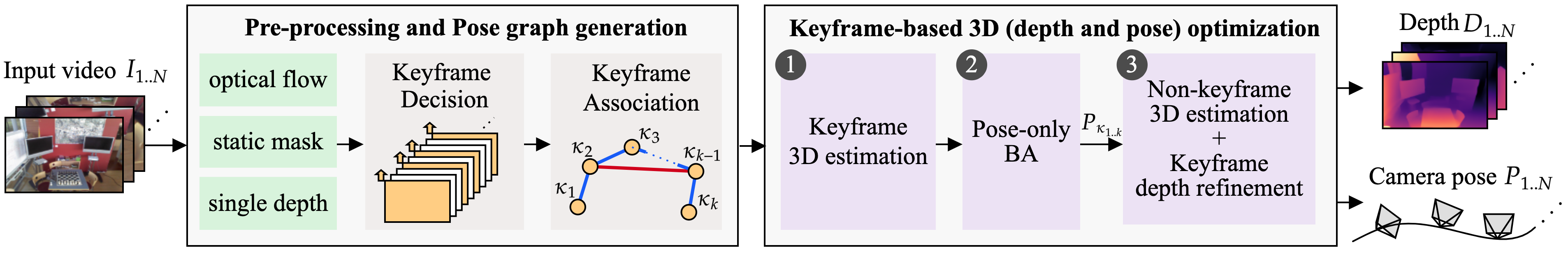
Figure 2: Pipeline overview. GCVD takes a monocular RGB video as input to estimate per-frame depth and pose. The pre-processing and pose graph generation stage (Sec. Pre-processing and Pose Graph Generation) first estimates adjacent optical flows and find static masks to filter likely-dynamic regions. It then uses single depths as prior for the optimization stage and constructs a pose graph by selecting the keyframes as vertices. The sequential (blue) and non-sequential (red) edges are thus formed via keyframe association. The optimization stage (Sec. Keyframe-based 3D Optimization) takes the estimations in the pre-processing stage as priors to optimize the depth and pose of input frames using the same Joint Optimization of Depth and Pose (Sec. Joint Optimization of Depth and Pose). The keyframe 3D estimation is followed by pose-only bundle adjustment (BA) for global consistency. The depth of keyframes and depth/pose of the remaining non-keyframes can then be optimized more efficiently through learning.

Related Work

Traditional Approach: Traditional SfM (Wu et al. 2011; Moulon et al. 2016; Schonberger and Frahm 2016) jointly estimate the 3D structure and camera poses of multi-view images via bundle adjustment (Agarwal, Mierle, and Others 2022; Kümmerle et al. 2011) on the local features. Subsequently, multi-view stereo (MVS) (Furukawa and Hernández 2015) following the estimated pose obtain dense depth but often yield holes and noises in general.

In another track, traditional visual odometry (VO) and SLAM (Klein and Murray 2007; Engel, Schöps, and Cremers 2014; Mur-Artal, Montiel, and Tardos 2015) usually maintain keyframes and a pose graph to perform efficient and consistent localization. Besides, bundle adjustment (BA) (Triggs et al. 1999) and pose graph optimization (Kümmerle et al. 2011) can be introduced to prevent drifts and enhance global consistency.

The performance of traditional methods generally rely on successful feature tracking. The sparse local features (Lowe 2004; Bay, Tuytelaars, and Van Gool 2006; Rublee et al. 2011) extracted are often fragile in various challenging conditions such as homogeneous areas, motion blur, and illumination changes. Hence, they are demanding to obtain dense depth maps and non-robust enough to handle the texture-less and blur situations for the videos in the wild.

Learning Depth Only (Given Pose): Supervised learning has been widely used for the ill-posed single depth estimation problem (Eigen, Puhrsch, and Fergus 2014; Liu et al. 2015; Eigen and Fergus 2015). Apart from acquiring real depth as groundtruth, some methods (Garg et al. 2016; Godard, Mac Aodha, and Brostow 2017; Gonzalez and Kim 2021) learn the single depth with binocular pairs. Other studies leverage synthetic data (Mayer et al. 2016) or pseudo groundrtuth (Chen et al. 2016; Li and Snavely 2018; Chen et al. 2020; Li et al. 2019b). MiDaS (Ranftl et al. 2020) obtains relative depth of stereo pairs from large-scale and diverse 3D movies. Recently, Miangoleh et al. (Miangoleh et al. 2021) integrate multi-scale depth of MiDaS to handle high-resolution images. Yin et al. (Yin et al. 2021) utilize point cloud networks to solve the perspective ambiguity of a single depth. Despite the single-depth methods show visual plausibility on individual depth maps, the issue of geometrical inconsistency among multi-views is not addressed.

With known camera poses, learning-based multi-view stereo can estimate dense depth of multiple images. In (Huang et al. 2018; Yao et al. 2018; Im et al. 2019), plane sweep algorithm is employed to estimate dense depth in a supervised manner. The methods in (Long et al. 2021; Wimbauer et al. 2021) estimate video depth with known camera pose or obtain the pose via COLMAP.

Depth and/or Pose Supervision and Joint Estimation: Approaches of this type utilize groundtruth depths and/or known-pose views for training; the obtained joint-depth/pose estimator is then applied to the test-scene sequences of unknown poses. For depth estimation, UNet-like models are used to perform per-pixel depth regression (Ummenhofer et al. 2017; et al. 2017; Zhou, Ummenhofer, and Brox 2018; Bloesch et al. 2018; Czarnowski et al. 2020). Deep cost volume with plane sweep structure are also adopted (Wei et al. 2020; Teed and Deng 2019; Wang et al. 2021). To estimate the pose, some methods directly use networks for regression (Ummenhofer et al. 2017; Zhou, Ummenhofer, and Brox 2018; Wei et al. 2020; Teed and Deng 2021); some others leverage the fundamental multi-view and epipolar geometry (et al. 2017; Bloesch et al. 2018; Teed and Deng 2019; Czarnowski et al. 2020; Wang et al. 2021). However, acquiring the groundtruth pose or depth in real world is non-trivial (e.g., requiring LiDAR (Saxena, Sun, and Ng 2008; Geiger et al. 2013) or RGB-D cameras (Sturm et al. 2012; Nathan Silberman and Fergus 2012; Shotton et al. 2013)). The demanding ability of generalization to the testing data of unknown scenes also restricts the usage in practice.

Self-Supervision for Depth and Pose: Methods in this category learn a joint depth/pose inference network in a self-supervised (or unsupervised) manner without relying on pre-given groundtruths (Zhou et al. 2017; Gordon et al. 2019; Godard et al. 2019; Chen, Schmid, and Sminchisescu 2019; Li et al. 2019a; Bian et al. 2019; Ranjan et al. 2019; Zou et al. 2020; Jiao, Tran, and Shi 2021; Watson et al. 2021; Zhou et al. 2021; Jung, Park, and Yoo 2021). They cooperatively regulate the depths and poses on monocular videos via warping-based view synthesis from the training data. Further approaches use optical flow (Yin and Shi 2018; Ranjan et al. 2019; Jiao, Tran, and Shi 2021) and segmentation (Casser et al. 2019; Ranjan et al. 2019) to improve the performance and handle dynamic objects. Yet, in test time, most networks still perform single-depth estimation and thus yield incoherent results. The methods also suffer from the generalization issue due to the domain gap between training and testing data.

Test-Time Training Approach: To avoid the difficulty of applying the inference model learned from given environment to unseen environment, test-time-training methods have been proposed more recently, making the solutions better for practical use. Despite the speed of test-time-training is slower than pure inference, the approaches meet the requirement of offline videos that need no real-time processing. CVD (Luo et al. 2020) is the first attempt toward test-time training to obtain geometrically consistent depth and pose estimation of a video. However, CVD relies on the SfM tool COLMAP which suffers from the fragile and sparse reconstruction and the computation is slow. Deep3D (Lee et al. 2021) uses a network-based optimization framework to learn video depth and pose for video stabilization, but the depth performance is restricted due to the lack of single depth prior. CVD2 (Kopf, Rong, and Huang 2021) uses a deformative mesh on single depth with a post-processing filter to show promising depth results; however, the pose performance still suffers from the bias of single depth as no fine-tuning mechanisms have been accommodated for the depth net. Besides, CVD2 requires tremendous optimization time. Its quantitative performance is only evaluated on the videos of 50 frames (Wulff et al. 2012).

Current works only ensure local consistency with nearby frames, whereas the global consistency is not tackled. We introduce GCVD that is the first test-time-training method with global consistency, which can obtain more accurate and robust results. Due to the global consistency, GCVD is scalable to long videos. In our experiments, 1000-frames videos are used to validate the performance.

Methodology

Given an $N$-frame video $I_{1..N}$, our goal is to estimate dense depth maps $D_{1..N}$ and camera poses $P_{1..N}$. Our CNN-based optimization framework utilizes the learning-based SfM to jointly estimate depth and pose of each frame. Nevertheless, applying SfM to a video may suffer from various challenges such as small camera baseline motion and lacking of co-visible scenes among frames.

Proper baselines arrangement: Current test-time-training solutions (e.g., Deep3D (Lee et al. 2021) and CVD2 (Kopf, Rong, and Huang 2021)) simply take near-to-distant neighbor frames with certain frame intervals empirically selected (e.g., 1, 2, 4, 8) to ensure a coherence baseline. The strategy does not take the real disparities between the frames into account, and does not guarantee the proper baselines among the frames for SfM. In our work, we leverage the recent progress of deep optical flow estimation, and introduce dense flow-guided keyframes to perform initial optimization with adequate baseline motions. The pipeline (Fig. 2) is introduced in Pre-processing and Pose Graph Generation and Keyframe-based 3D Optimization and the network-based optimization module is elaborated in Joint Optimization of Depth and Pose.

Pre-processing and Pose Graph Generation

Videos often contain motion blurs and large view-direction changes, yielding failures of traditional sparse features on matching. We use learning-based optical flows among video frames to overcome this difficulty and obtain dense flow maps. However, in contrast to existing approaches CVD2 and Deep3D which need the computation of flows from a target frame to many other frames, our GCVD initially estimates the depth and pose of keyframes with reliable camera baselines and then enforces global optimizations later; thus, we can only take the flow of adjacent views (i.e., $\hat{F}^{t}_{t\pm 1}$) to save the computation burden.

Besides, to prevent dynamic objects from disturbing pose estimation, semantic segmentation (e.g., Mask-RCNN in Detectron2 (Wu et al. 2019)) is used to obtain a binary mask $\hat{M}_{t}$ that filters out the likely-dynamic pixels in each frame $I_{t}$. We also take the single depths of MiDaS (Ranftl et al. 2020) as the depth prior to regularize the optimization.

The ideas of keyframe and pose graph have been widely used in traditional SLAM (Klein and Murray 2007; Engel, Schöps, and Cremers 2014; Mur-Artal, Montiel, and Tardos 2015) and SfM (Schonberger and Frahm 2016; Barath et al. 2021) to reduce the computational complexity and ensure global consistency for large-scale reconstruction. Our method constructs a pose graph. Nevertheless, unlike traditional SLAM or SfM, we use learning-based approach to provide better robustness in the optimization. The pose graph has $k$ keyframes ($\kappa_{1..k}$) as its vertices, and the edges of the graph include the sequential edges and the non-sequential co-visible edges, as depicted below.

Dense-flow-guided keyframe decision. To sample representative keyframes from videos, traditional solutions rely on sparse feature tracking while long feature tracks are challenging to obtain. Instead, the dense optical flow acquired in the pre-processing can provide a reliable reference for keyframe decision. Thus, the frame $I_{t}$ is chosen as a keyframe if the accumulated flow magnitude $\bar{F}^{\kappa^{*}}_{t}$ from the last selected keyframe $\kappa^{*}$ exceeds a movement threshold $\Delta$.

$$\bar{F}^{\kappa^{*}}_{t}=\sum^{t-1}_{i=\kappa^{*}}\left(\frac{1}{|\hat{M}_{i}|}\sum_{x\in\hat{M}_{i}}\|\hat{F}^{i}_{i+1}\|_{2}\right),$$ (1)

where we set $\Delta=0.1$ and only use the static regions $\hat{M}$ for evaluation. Then, the flow of adjacent keyframes, $\hat{F}^{\kappa_{i}}_{\kappa_{i\pm 1}}$, are established for the keyframe optimization. As we use the accumulated adjacent flows to pick just-needed frames, compared to uniform selection, a more compact and exemplary keyframe set can be built. After selecting $k$ keyframes, the sequential edges are formed by connecting the keyframes of nearby indices within a subset of $\kappa_{i\pm\alpha}$ in the pose graph to ensure local consistency. For those keyframe pairs with the index differences exceeding $\alpha$, we will consider their co-visibility of shared scenes to form the further edges of non-sequential co-visible views to enforce better the global consistency.

CNN-based keyframe association. The keyframe pairs with high image similarities are picked and geometrically verified to serve as non-sequential co-visible edges. We leverage the deep features of the $k$ keyframes and compute their cosine similarity one-by-one to form a similarity matrix $A_{k\times k}$. For each keyframe, the feature is extracted by an ImageNet-pretrained ResNet encoder (Godard et al. 2019). The output feature is then passed through a global average pooling layer and $L2$ normalization. Thus, $A_{k\times k}$ can be simply computed by the inner-product of the $k$ normalized feature vectors. Then, the associated pairs are sampled from $A$ by a similarity threshold $\delta$ ($=0.9$) and max-pooling for reducing redundant pairs.

Besides, the geometric verifications are necessary to filter the noisy associated keyframe pairs. Traditional verifications utilize the inlier ratio of estimated fundamental matrix or homography via SIFT (Lowe 2004) and RANSAC (Fischler and Bolles 1981), while it is not reliable enough. We additionally examine the forward-backward consistency of the dense optical flow of each associated pair. Moreover, to guarantee adequate co-visible areas for optimization, the associated pairs are removed if the average flow magnitude exceeds the movement threshold $\Delta$ of keyframe decision.

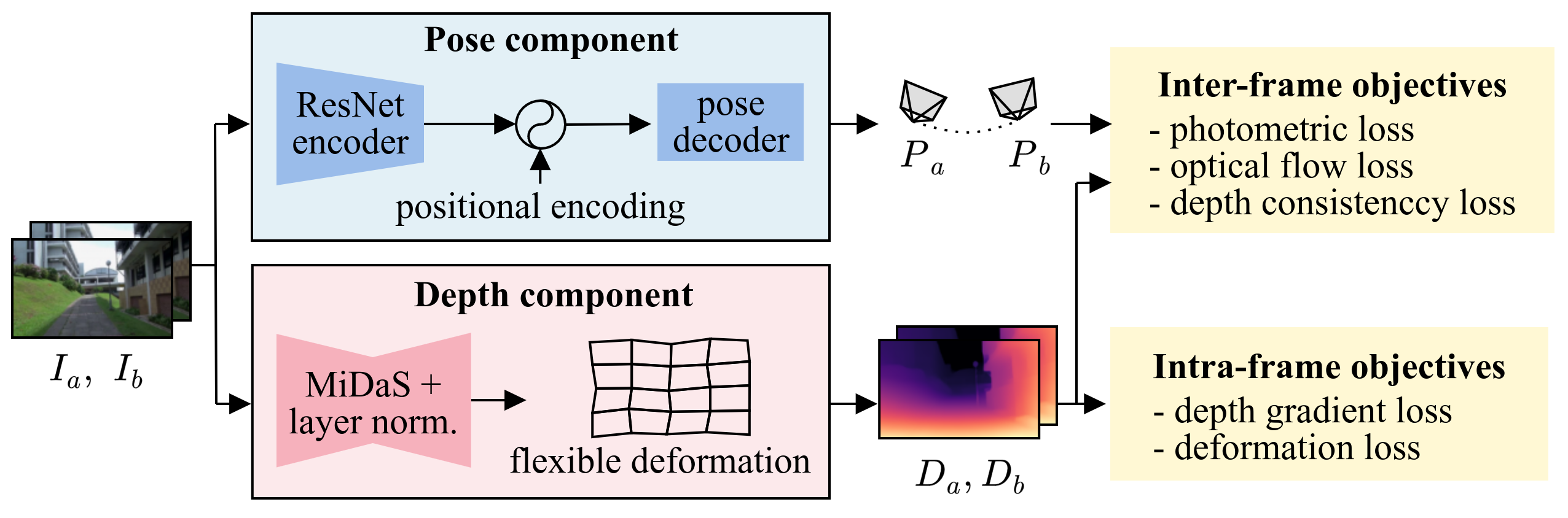
Figure 3: Joint optimization of depth and pose. The 3D optimization module takes a set of frame pairs as input to estimate the depths and poses. The depth component adopts MiDaS (Ranftl et al. 2020) with an additional layer normalization and a learnable mesh deformation (Kopf, Rong, and Huang 2021). The pose component consists of ResNet-based encoder-decoder (Godard et al. 2019) with a positional encoding (Vaswani et al. 2017) to encourage better convergence. Both Steps 1 and 3 in the Keyframe-based 3D Optimization stage of Fig. 2 use this module for learning.

Keyframe-based 3D Optimization

The proposed pipeline performs keyframe optimization with suitable camera movement to achieve robust estimation as initials. Then, pose graph optimization is utilized to retain global consistency of keyframes’ pose estimations. Finally, the depth and pose of the remaining frames are estimated efficiently according to the pose graph obtained. In the following, we give an overview of the procedures. Details of our joint depth-and-pose deep network model is depicted in Joint Optimization of Depth and Pose.

Keyframe 3D estimation via deep model. For each keyframe $\kappa_{i}$, the depth and pose are learned with multiple nearby keyframes of $\kappa_{i\pm\tau}$ (i.e., the sequential edges in pose graph) with a descending weight $\frac{1}{\tau}$ to acquire consistent results. Besides, a mini-batch of keyframes are optimized simultaneously with a GPU. Thus, the mini-batches are overlapped with the interval $\tau$ to ensure coherent solutions (Lee et al. 2021). In our work, we set $\tau\in\{1,2,4,8\}$. The relative poses obtained for sequential edges are then recorded for the next pose-only bundle adjustment. Likewise, we optimize the non-sequential co-visible keyframe pairs (without decreasing weights) and obtain the their relative poses accordingly. Hence, each edge of the pose graph is set up with an initial relative-pose transformation.

Global pose graph optimization with efficiency. The pose graph optimization (Kümmerle et al. 2011) is used to refine the pose estimations of keyframes from the above initialization. Note that we perform pose-only bundle adjustment for $P_{\kappa_{1..k}}$ rather than depth and pose bundle adjustment for efficiency. Instead, the depths of keyframes are fine-tuned in the next step leveraging the learning models. The extensive bundle-adjustment overhead can thus be shared with deep networks that are cooperated to yield a more efficient optimization.

Non-keyframe 3D optimization and keyframe depth refinement. Besides fine-tuning the keyframe depth, the remaining non-keyframes are optimized with the fixed keyframe poses (i.e., $P_{\kappa_{1..k}}$) over fewer iterations via the deep network. Likewise, $(D_{t},P_{t})$ of each frame is optimized with multiple nearby views $t\pm\tau$. We then obtain the depth $D_{1..N}$ and pose $P_{1..N}$ of the entire video.

Joint Optimization of Depth and Pose

In this section, we introduce the optimization module for 3D estimation. Our approach leverages the deep networks to save the scene information in the model weights to facilitate sequential fragments optimization. The module takes a set of frame pairs as input and estimate the depths and poses simultaneously. For simplicity, we depict the module with a pair of images $(I_{a},I_{b})$ as input. More pairs simply use the sum of respective loses. The networks learn both depth and pose to obtain the the output $D_{a}$, $D_{b}$, $P_{a}$, $P_{b}$ with the objectives designed below.

Depth and pose components. As shown in Fig. 3, the depth and pose components estimate the individual depth $D_{t}$ and 6-DoF global pose $P_{t}$, respectively, associated with an input RGB frame $I_{t}$. The depth component exploits a MiDaS-pretrained network (Ranftl et al. 2020) with an additional layer normalization to stabilize the output scale of depth estimation. Then, a learnable mesh deformation (Kopf, Rong, and Huang 2021) is adopted to achieve better alignments among sequential depths. Unlike CVD2 (Kopf, Rong, and Huang 2021) that directly takes fixed single depths as initials, we use a trainable depth network that can refine the bias of the initial depth to encourage better estimations. While due to the time and space efficiency, only the last two convolutional layers of MiDaS network are used to learn a larger span of frames at a time.

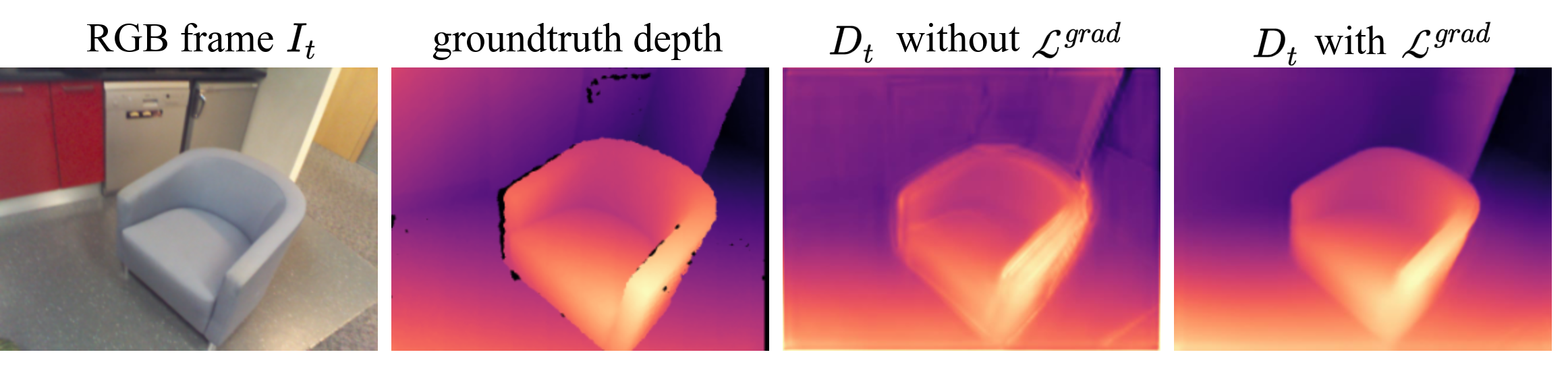
Figure 4: Depth gradient loss $\mathcal{L}^{grad}$ retains the depth prior of initial single depth (Ranftl et al. 2020). The result without $\mathcal{L}^{grad}$ may introduce blurring after updating the depth component.

The pose component adopts the PoseNet (Godard et al. 2019) based on ResNet encoder (He et al. 2016). Similar to the depth component, the pose encoder is frozen with ImageNet-pretrained weights and only the decoder can be optimized. The information saved in the learned weights of the decoder can help boost the convergence for the next optimization. Moreover, the feature map is added with a positional encoding (Vaswani et al. 2017) which encodes the chronological order of the entire sequence to enhance the learning for the sequence.

Method	known pose?	Depth Metrics				Pose Metrics
		AbsRel$\downarrow$	SqRel$\downarrow$	RMSE$\downarrow$	$\delta<$	ATE	RPE Trans	RPE Rot
					$1.25\uparrow$	(m)$\downarrow$	(m) $\downarrow$	(deg) $\downarrow$
DPSNet$\dagger$ (Im et al. 2019)	✓	0.199	0.142	0.438	0.710	-	-	-
CNMNet$\dagger$ (Long et al. 2020)	✓	0.161	0.083	0.361	0.766	-	-	-
NeuralRecon$\dagger$ (Sun et al. 2021)	✓	0.155	0.104	0.347	0.820	-	-	-
DeepV2D (Teed and Deng 2019)		0.162	0.092	0.380	0.767	0.471	1.018	60.979
DROID-SLAM (Teed and Deng 2021)		0.209	0.132	0.462	0.665	0.463	0.928	40.143
Deep3D (Lee et al. 2021)		0.172	0.105	0.406	0.748	0.310	0.306	8.665
CVD2 (Kopf, Rong, and Huang 2021)		0.154	0.085	0.379	0.795	0.375	0.517	31.102
Ours (GCVD)		0.124	0.054	0.307	0.858	0.249	0.257	8.155

Table 1: Quantitative evaluations of depth and pose on 7-Scenes dataset (Shotton et al. 2013). The standard depth evaluation measures per-frame errors and accuracy metrics. The pose evaluation computes the per-sequence pose errors. $\dagger$We also refer to the approaches of multi-view stereo and 3D reconstruction with known camera pose and compare with the results reported in NeuralRecon (Sun et al. 2021).

Objectives. The proposed objectives include inter-frame constraints for geometrical consistency and intra-frame regularization. The inter-frame objectives ensure consistent estimations between two views. The test-time learner exploits the point transformation between $(I_{a},I_{b})$ via 3D projection as formulated below:

$$\tilde{x}_{b}\sim KP_{b}P_{a}^{-1}D_{a}(x_{a})K^{-1}\tilde{x}_{a},$$ (2)

where $\tilde{x}_{a}$ and $\tilde{x}_{b}$ denote the homogeneous form of a pixel in $I_{a}$ and $I_{b}$, respectively. $K$ stands for the camera intrinsics. Accordingly, the rigid flow $F^{b}_{a}=x_{b}-x_{a}$ is used to realize the inter-frame constraints in the following three aspects.

The photometric loss computes the appearance bias between $I_{a}$ and the synthesized $I^{b}_{a}$ (warped using $F^{b}_{a}$) by $L_{1}$ and structure dissimilarity (Wang et al. 2004) losses:

$$\mathcal{L}^{photo}_{a,b}=\frac{1}{|V^{b}_{a}|}\sum_{x\in V^{b}_{a}}\|I^{b}_{a}-I_{a}\|_{1}+DSSIM(I^{b}_{a},I_{a}),$$ (3)

where $V^{b}_{a}$ denotes the valid points projected from $I_{b}$ onto the image plane of $I_{a}$ and excluding likely-dynamic pixels by $\hat{M}_{a}$.

The optical flow loss measures the displacement error in the image space. Hence, the flow $\hat{F}$ generated in the pre-processing is used as the supervision for the rigid flow $F$. We examine the forward-backward consistency between the pre-processing flows $\hat{F}^{b}_{a}$ and $\hat{F}^{a}_{b}$ to form a binary mask $\tilde{V}^{b}_{a}$, and let $\hat{V}^{b}_{a}=\tilde{V}^{b}_{a}\cap V^{b}_{a}$.

$$\mathcal{L}^{flow}_{a,b}=\frac{1}{|\hat{V}^{b}_{a}|}\sum_{x\in\hat{V}^{b}_{a}}\|F^{b}_{a}-\hat{F}^{b}_{a}\|_{1}.$$ (4)

The depth consistency loss $\mathcal{L}^{const}$ (Bian et al. 2019) assesses the inconsistency between individually estimated depth $D_{a}$ and $D_{b}$.

$$\mathcal{L}^{const}_{a,b}=\frac{1}{|V_{a}|}\sum_{x_{a}\in V_{a}}\frac{\|D^{b}_{a}-D_{a}\|_{1}}{D^{b}_{a}+D_{a}},$$ (5)

where $D^{b}_{a}$ is the transformed depth of $I_{a}$ using $D_{b}$, $P_{b}P_{a}^{-1}$.

Apart from inter-frame losses, the intra-frame objectives are utilized to regularize each depth $D_{t}$, including the dynamic areas. We conduct the depth gradient loss $\mathcal{L}^{grad}_{t}$ to preserve the depth prior from pre-computed MiDaS depth $\hat{D}_{t}$. The optimization can refine the bias of initial single depth. Thus, the single depth $\hat{D}_{t}$ obtained in the pre-processing is exploited to provide the supervision of depth edge (Fig. 4). Let $\nabla D^{s}_{t}(x)$ denote the 2D gradient vector of pixel $x$ in the downsampled depth map $D_{t}^{s},s\in\{0,1,2\}$. We measure the orientation difference of depth gradients to avoid scale difference between $\hat{D}_{t}$ and $D_{t}$.

$$\mathcal{L}^{grad}_{t}=\sum_{s}\sum_{x}\left(1-\frac{\nabla D^{s}_{t}(x)\cdot\nabla\hat{D}^{s}_{t}(x)}{\|\nabla D^{s}_{t}(x)\|_{2}\|\nabla\hat{D}^{s}_{t}(x)\|_{2}}\right)^{2}.$$ (6)

The regularization of deformation proposed by Kopf et al. (Kopf, Rong, and Huang 2021) maintains the spatial smoothness of learnable mesh for a flexible deformation. Likewise, we use the regularization loss $\mathcal{L}^{deform}_{t}$ to encourage smoothness in dynamic area $1-\hat{M}_{t}$. Finally, the total loss $\mathcal{L}$ of a pair of $(I_{a},I_{b})$ is conducted as:

$$\mathcal{L}= \lambda^{photo}\mathcal{L}^{photo}+\lambda^{flow}\mathcal{L}^{flow}+\lambda^{const}\mathcal{L}^{const}$$

$$+\lambda^{grad}\mathcal{L}^{grad}+\lambda^{deform}\mathcal{L}^{deform},$$

where the inter-frame objectives compute the bidirectional losses and the intra-frame objectives sum up the losses of individual frames. The weights $\lambda^{photo}$, $\lambda^{flow}$, $\lambda^{const}$, $\lambda^{grad}$, $\lambda^{deform}$ are set as $1,10,0.5,0.1,0.5$, respectively. Note that $\mathcal{L}^{flow}$ is used only when $I_{a}$ and $I_{b}$ are adjacent.

Figure 5: Visual comparisons with state-of-the-art on 7-Scenes (Shotton et al. 2013). The 3D point cloud is back-projected from a view with the estimated depth. Deep3D (Lee et al. 2021) produces in weak depth results and even collapse (constant value). CVD2 (Kopf, Rong, and Huang 2021) results in poor pose performance (observed via the bad alignment of the green and blue trajectories) despite the plausible depth. Our method shows the most favorable performance on both depth and pose. Zoom in for more detailed visualization is suggested.

Implementation Detail

The approach is realized in PyTorch with Adam and g2o library (Kümmerle et al. 2011). The resolution of depth and deformation mesh are 384 and 17, respectively, following CVD2 (Kopf, Rong, and Huang 2021) for the longer side of frame. RTX3090 GPU is used on the mini-batch size 40. We run the optimizations of sequential keyframes, non-sequential keyframes, and non-keyframes with 300, 100 and 100 iterations, respectively. We further perform flow-guided depth filter like CVD2 (Kopf, Rong, and Huang 2021) as post-processing. The optical flow (Teed and Deng 2020) is used. More details are given in the appendix.

Experiments

We compare the proposed method with the SOTA test-time-training methods, CVD2 (Kopf, Rong, and Huang 2021) and Deep3D (Lee et al. 2021). CVD2 jointly optimizes pose and learnable deformation from initial MiDaS (Ranftl et al. 2020) depths. Deep3D takes DepthNet and PoseNet (Godard et al. 2019) and learns from ImageNet pretrained weight to acquire depth and pose. For fair comparisons, we assume an ideal camera intrinsic and re-implement Deep3D with the same resolution of depth, optical flow estimation (Teed and Deng 2020) and static masks as CVD2 and ours. In addition, we compare our approach with the SOTA supervised SLAM systems (Teed and Deng 2019, 2021), where the SLAM mode of DeepV2D (Teed and Deng 2019) performs pose optimization in a tracking window and DROID-SLAM (Teed and Deng 2021) utilizes dense bundle adjustment to achieve global consistency.

Datasets. In contrast to CVD2 conducting evaluations on synthetic video clips (with each only 50-frames long) of Sintel dataset (Wulff et al. 2012), We conduct the experiments on long sequences (500 to 3000 frames) of real-world datasets.

$\bullet$ 7-Scenes RGB-D dataset (Shotton et al. 2013) has 46 sequences with either 500 or 1000 frames. The indoor scenes are grabbed with a Kinect camera at size 640$\times$480.

$\bullet$ TUM RGB-D dataset (Sturm et al. 2012) is gathered by a handheld Kinect camera with more demanding cases such as texture-less area and abrupt motions. Seven representative sequences (613$\sim$2965 frames) in TUM RGB-D are used for evaluation.

$\bullet$ EuRoC dataset (Burri et al. 2016) has 11 sequences (1710$\sim$3682 frames) filmed by a micro aerial vehicle. We demonstrate the comparisons in our appendix.

Evaluation metrics. We follow the standard depth evaluation (Eigen, Puhrsch, and Fergus 2014) to align the scales between the estimated and groundtruth depths by median scaling. The pose evaluation uses the metric of visual odometry (Sturm et al. 2012; Zhang and Scaramuzza 2018), including absolute trajectory error (ATE) and relative pose error (RPE) with 7-DoF alignment.

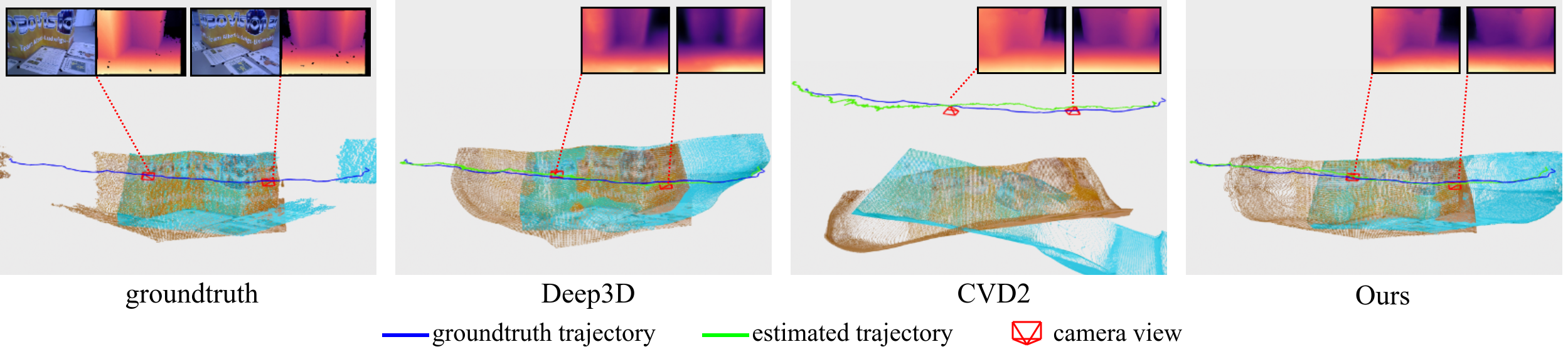
Figure 6: Visual comparisons of geometric consistency. Visualizing the geometric consistency via the point clouds between two distant views (200-frames interval). As shown in the groundtruth, the back-projected point clouds (brown and cyan) from two views are supposed to align in the co-visible area. Our GCVD and Deep3D (Lee et al. 2021) maintain better geometric consistency and show promising alignments of point clouds, while CVD2 (Kopf, Rong, and Huang 2021) results in severe misalignment between the distant views.

Sequence	Pose Error (ATE in meters) $\downarrow$				Depth Error (Abs Rel) $\downarrow$
	COLMAP	Deep3D	CVD2	GCVD	Deep3D	CVD2	GCVD
fr1_desk	0.019	0.580	0.273	0.229	0.1940	0.1090	0.0940
fr1_desk2	0.027	0.611	0.314	0.156	0.2282	0.1139	0.1305
fr2_desk	0.818	0.260	0.613	0.422	0.0973	0.1544	0.1130
fr3_cabinet	failed	1.225	0.444	0.850	0.4613	0.1236	0.1832
fr3_nstr_tex_near_loop	0.015	0.694	0.491	0.399	0.2437	0.0615	0.0352
fr3_sitting_static	0.033	0.006	0.029	0.006	0.2368	0.1260	0.1243
fr3_str_tex_far	0.008	0.089	0.169	0.131	0.0511	0.0742	0.0810
Mean	0.153	0.495	0.333	0.313	0.2160	0.1089	0.1087

Table 2: Quantitative evaluation on TUM RGB-D (Sturm et al. 2012). We present the depth and pose errors of each sequence and compare with Deep3D (Lee et al. 2021), and CVD2 (Kopf, Rong, and Huang 2021). We additionally provide the pose results of COLMAP (Schonberger and Frahm 2016) as reference.

Evaluation on 7-Scenes (Shotton et al. 2013)

Table 1 shows the quantitative comparisons of our approach to the SOTA methods. Although DeepV2D (Teed and Deng 2019) and DROID-SLAM (Teed and Deng 2021) utilize pose graph for the pose refinement and bundle adjustment in testing, they are restricted by the generalization capability of supervised learning in different datasets. Test-time training approach Deep3D (Lee et al. 2021) shows the second best pose performance; however, it results in worse depth estimation. CVD2 (Kopf, Rong, and Huang 2021) maintains more depth priors from MiDaS while the bias in the depth prior leads in poor pose estimation. Besides, we compare our GCVD with other depth-estimation approaches with known camera pose. The quantitative depth scores of DPSNet (Im et al. 2019), CNMNet (Long et al. 2020), and NeuralRecon (Sun et al. 2021) are provided by (Sun et al. 2021). Similar to DeepV2D and DROID-SLAM, the supervised methods with known pose may still suffer from the domain discrepancy between training and test data. In contrast, the proposed GCVD achieves globally consistent optimization on test data and demonstrates the best performance on both standard depth and pose metrics.

We conduct visual comparisons by displaying the back-projected point clouds and the pose estimation with the groundtruth trajectory by 7-DoF alignment (Zhang and Scaramuzza 2018). As shown in Fig. 5, although Deep3D demonstrates some promising camera estimations, it is prone to collapse on the depth estimation. CVD2 provides plausible depths with the aids of MiDaS while yields weak pose results due to the lack of global consistency. Again, our method reveals better results in 3D visualization.

Evaluation on TUM-RGBD (Sturm et al. 2012)

In this experiment, we compare our GCVD with the test-time training approaches (CVD2 and Deep3D) and also COLMAP which is a traditional representative solution having maintaining global consistency. Table 2 provides the per-sequence quantitative errors. We only present the pose results of COLMAP since its dense depths via multi-view stereo still contain holes and noises. Although COLMAP shows superior pose results, it completely fails (collapses) in a sequence (marked as red in Table 2) due to the fragile sparse reconstruction. As for test-time training, our method attains the lowest depth and pose errors in overall. We handle depth prior properly with the learnable networks to facilitate pose learning. Thus, our approach shows better pose estimation on most sequences compared with CVD2, which accumulates more pose errors for long sequences. Our GCVD can refine the long pose estimation for maintaining global consistency. On the other hand, we find the weak pose performance of some sequences affected by the unreliable pre-computed optical flow, which will be discussed in the limitations of our approach in the appendix.

Besides, we compare the geometric consistency by visualizing the alignment of point clouds from different views. The two distant frames viewing the common scenes are back-projected the 3D point clouds. Hence, the geometric inconsistency can be seen by the misalignment between the two point clouds in the co-visible area. As shown in Fig. 6, Deep3D and ours show similar point cloud alignments to the groundtruth’s because both approaches have the depth fine-tuning mechanisms. Nevertheless, the accumulated depth bias leads CVD2 to yield poor pose estimation and large misalignment between the views.

Ablation studies

We conduct ablation studies on 7-Scenes dataset (Shotton et al. 2013) in Table 3. For the depth component, the inserted layer normalization stabilizes the depth scale of MiDaS (Ranftl et al. 2020) network and hence facilitates the depth and pose performance by 35% and 40%, respectively. The flexible deformation (Kopf, Rong, and Huang 2021) regulates the spatial misalignments of each depth to improve depth estimation by 4%. Besides, the depth gradient loss retains the initial depth priors during refining the depth bias. The well-handled depth prior can encourage a better joint optimization, thus reducing the pose errors by 15% (0.327 to 0.277). Moreover, the method without the keyframe strategy raises 11% pose error (0.277 to 0.308) due to the lack of proper camera baselines for initial optimization. Finally, the pose graph optimization for global consistency further cuts down the pose error by 10% (0.277 to 0.249).

Ablation settings					Errors $\downarrow$
KF	layer	mesh	grad.	PGO	Depth	Pose
	norm	deform.	loss		AbsRel	ATE
✓					0.208	0.555
✓	✓				0.137	0.332
✓	✓	✓			0.132	0.327
✓	✓	✓	✓		0.125	0.277
	✓	✓	✓		0.127	0.308
✓	✓	✓	✓	✓	0.124	0.249

Table 3: Ablation studies on 7-Scenes (Shotton et al. 2013). We validate the effectiveness of the keyframe strategy (KF), the added layer normalization and mesh deformation in the depth component, depth gradient loss, and pose graph optimization (PGO) in our pipeline.

Runtime comparisons

We compare the runtime of our GCVD with the test-time-training methods. We select five long videos and extract the first $n$ frames of the videos to compose different lengths of sequences for runtime evaluation. The execution times of the videos are measured on an i7-11700K with a RTX3090 GPU. We present the averaged per-frame time in Table 4. Note that we do not compare with COLMAP which requires extremely expensive time (e.g., $\sim$56 secs for each frame on a 2000-frame video). CVD2 shows about 6 to 9 times slower than our method due to the preparation of multiple pairs of optical flow and the traditional optimizer with CPU. Deep3D provides strong efficiency in long videos; however, it tends to yield drifts and collapse in depth estimation. In contrast, our method performs fastest in short videos by learning few keyframes first then optimizing the non-keyframes with fewer iterations. For long videos, our GCVD is slightly slower than Deep3D due to keyframe association on more keyframes for global consistency.

# frames	50	200	500	1000	2000
CVD2	13.90	14.83	17.34	21.73	26.13
Deep3D	4.13	3.03	2.75	2.66	2.61
GCVD	2.40	2.53	2.74	2.83	3.04

Table 4: Runtime comparison. We compute the per-frame runtime (sec) in different lengths of videos. Our method shows the fastest speed in short videos and achieves a good trade-off between efficiency and global consistency compared with Deep3D.

Conclusion

We present GCVD, a learning-based method for video depth and pose estimation with global consistency and efficiency. To our knowledge, this is the first study tackling global consistency for test-time training. Based on the global poses of keyframes from the pose-only bundle adjustment, the deep networks jointly learn keyframe depth refinement and the depth and pose of the remaining frames efficiently. In addition, our proposed method can better handle single depth prior properly and fine-tune the depth network to alleviate depth bias and achieve robust and consistent 3D estimation. Experimental results show that GCVD outperforms the state-of-the-art approaches on both depth and pose evaluation. Moreover, GCVD achieves high efficiency by keeping the scene knowledge in network weights to boost the optimization of next fragment of frames. We will release our codes to public. In contrast to COLMAP that uses traditional techniques, our GCVD is a fundamental deep-learning tool for the offline-video SfM.

Appendix A Appendix

We present GCVD, a test-time training method for video-based 3D estimation based on offline videos. There are still few test-time training studies for video-based SfM. Existing approaches are, however, robust to only local consistency for video depth estimation. Our approach is the first global-consistency solution to this direction. It needs only light-weight pose-only bundle adjustment as initial, and then takes advantage of neural-networks learning for global optimization of poses and depths simultaneously. Our GCVD can serve as a generally useful tool for offline video-based SfM (like the renowned tool COLMAP using traditional approach), where it can provide dense 3D estimations instead of fragile or sparse 3D outputs for challenging conditions such as homogeneous areas and motion blurs. Compared to the representative test-time-training approaches (such as CVD2 (Kopf, Rong, and Huang 2021)), our approach can handle long videos at reasonable runtime. Unlike the approach of (Kopf, Rong, and Huang 2021) that only validates the performance using 50-frames video clips, we validate the performance for 500$\sim$3682 frames, which considerably boosts the validation to practically useful situations.

In this appendix, we present additional details to complement our main paper, including implementation details, comparisons with the state-of-the-art SLAM approaches, evaluation on EuRoC dataset (Burri et al. 2016), runtime analysis, and limitations of our GCVD.

Implementation Detail

Keyframe-based pose graph optimization. We perform pose graph optimization with g2o (Kümmerle et al. 2011) for globally consistent pose estimation. The edges of the pose graph include sequential and non-sequential edges. Each sequential edge $e_{i,i\pm\tau},\tau\in\{1,2,4,8\}$ of the pose graph connects the keyframe pair $(\kappa_{i},\kappa_{i\pm\tau})$ with the relative pose $P^{-1}_{\kappa_{i}}P_{\kappa_{i}\pm\tau}$ and the weight matrix $diag(\frac{1}{\tau})$ to ensure temporal coherence in a local range. The sequential edges contain relatively nearby views determined by the optical-flows. However, in addition to the sequential edges, there could be farther views which share co-visible scenes. Hence, we also establish the non-sequential edges via keyframe association, which connects the keyframe pairs with the index differences exceeding $\alpha=\max(\tau)$ but sharing a co-visible scene to enhance global consistency. Similarly, the non-sequential co-visible edges are constructed with the optimized relative poses and identity weight matrices. The pose graph optimization is conducted with at most 100 iterations to obtain global pose estimation $P_{\kappa_{1..k}}$. Afterward, the depth and pose of the remaining frames and the depth of keyframes are estimated simultaneously with the frozen keyframe poses to maintain global consistency. Figure 7 demonstrates the effectiveness of the pose graph optimization for achieving the global consistency.

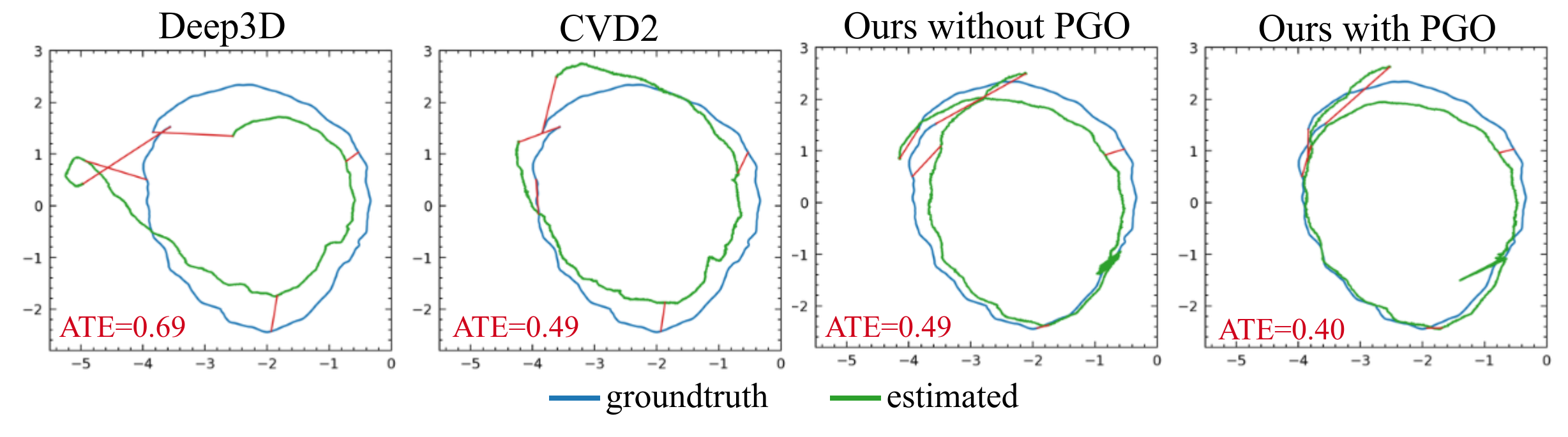
Figure 7: Visualization of global consistency. Our method reduces 18% pose error by using pose graph optimization (PGO) on the sequence fr3_nstr_tex_near_loop in TUM RGB-D dataset (Sturm et al. 2012).

Detail of joint depth and pose optimization. The test-time optimization framework is implemented in PyTorh with Adam (with $\beta_{1}=0.9$, $\beta_{2}=0.999$). The learning rates for sequential keyframes, non-sequential keyframes, and non-keyframes are $2\times 10^{-4}$, $5\times 10^{-5}$, and $1\times 10^{-4}$, respectively. To speed up the optimization, we compute the loss with a quarter scale of depth estimation in the keyframe optimization. Thus, the depth of keyframes will be further refined in the non-keyframe optimization with original scale (i.e., 384 for the longer side of the frame).

Post-processing. We follow the flow-guided depth filter proposed in CVD2 (Kopf, Rong, and Huang 2021) to further enhance the temporal consistency of edge details in depth maps. The final filtered depth $\tilde{D}_{t}$ acquires the depth details from neighboring depths $D_{t-\Omega..t+\Omega}$ ($\Omega=4$) with the chaining optical flow $\tilde{F}$.

$$\tilde{D}_{t}=\sum_{i=t-\Omega}^{t+\Omega}\omega_{i\to t}D_{i\to t},$$ (7)

where $D_{i\to t}$ is the projected depth of $I_{t}$ by transforming $D_{i}$ with $P_{t}$, $P_{i}$ and the chaining flow $\tilde{F}_{i\to t}$ to align the pixel coordinate. The maximum span $\Omega$ is set as 4 by default, and the weight term $\omega_{i\to t}$ considers both the depth reprojection error and the forward-backward inconsistent error of the chaining flow as follows:

$$\omega_{i\to t}=\exp\left(-\gamma_{1}\frac{\max(D_{t},D_{i\to t})}{\min(D_{t},D_{i\to t})}-\gamma_{2}\tilde{F}^{diff}_{i\to t}\right),$$ (8)

where $\tilde{F}^{diff}_{i\to t}$ denotes the forward-backward inconsistency between the chaining flow $\tilde{F}_{i\to t}$ and $\tilde{F}_{t\to i}$. The $\gamma_{1}=2$ and $\gamma_{2}=0.1$ balance the strength of the temporal depth filter. In the end, the final consistent depth $\tilde{D}_{1..N}$ and pose $P_{1..N}$ of the entire video $I_{1..N}$ is accomplished.

Table 5: Comparison with learning-based SLAMs on 7-Scenes (Shotton et al. 2013) and TUM RGBD dataset (Sturm et al. 2012).

Dataset	Method	Depth Metrics				Pose Metrics
		AbsRel$\downarrow$	SqRel$\downarrow$	RMSE$\downarrow$	$\delta<$	ATE	RPE Trans	RPE Rot
					$1.25\uparrow$	(m)$\downarrow$	(m) $\downarrow$	(deg) $\downarrow$
7-Scenes	DeepV2D (Teed and Deng 2019)	0.162	0.092	0.380	0.767	0.471	1.018	60.979
	DROID-SLAM (Teed and Deng 2021)	0.209	0.132	0.462	0.665	0.463	0.928	40.143
	Ours	0.124	0.054	0.307	0.858	0.249	0.257	8.155
TUM RGBD	DeepV2D (Teed and Deng 2019)	0.166	0.153	0.648	0.745	0.460	1.360	60.479
	DROID-SLAM (Teed and Deng 2021)	0.214	0.211	0.778	0.639	0.013	1.327	50.794
	Ours	0.109	0.077	0.461	0.858	0.313	0.277	15.919

Comparison with SOTA learning-based SLAMs

Although the SLAM approach reconstructs depth and pose from online (streaming) videos, which is different from our problem setting of video SfM for offline videos, we compare with the state-of-the-art supervised SLAMs (Teed and Deng 2019, 2021) which tackle global consistency. DeepV2D (Teed and Deng 2019) performs global pose optimization with a tracking window of eight frames. DROID-SLAM (Teed and Deng 2021) utilizes dense and full bundle adjustment to achieve global consistency. Table 5 presents the quantitative comparison on 7-Scenes (Shotton et al. 2013) and TUM RGBD (Sturm et al. 2012) datasets. Though DROID-SLAM achieves a superior score on the pose metric of Absolute Trajectory Error (ATE) on TUM RGBD, it shows the deficiency on the other pose metric, Relative Pose Error (RPE), which is used for measuring the drift. Both DeepV2D and DROID-SLAM are supervised methods trained on other datasets with groudtruth depth or pose. They suffer from generalization ability due to domain discrepancy and thus result in weak results on 7-Scenes dataset. In contrast, our test-time training approach directly learns on the input test video to address the generalization issue and achieves the best scores on 7-Scenes.

Comparison with ORB-SLAM2 (Mur-Artal, Montiel, and Tardos 2015)

We also compare GCVD with the traditional state-of-the-art SLAM approach ORB-SLAM2 (Mur-Artal, Montiel, and Tardos 2015), which performs loop closure to retain globally consistent poses and 3D map. Table 6 shows the pose comparisons with traditional COLMAP (Schonberger and Frahm 2016) and ORB-SLAM2 (Mur-Artal, Montiel, and Tardos 2015) on TUM RGBD dataset (Sturm et al. 2012). In general, ORB-SLAM2 shows the most accurate pose results with sparse hand-crafted features. Nonetheless, the sparse 3D reconstruction cannot provide complete dense depth for various video processing applications. Moreover, COLMAP and ORB-SLAM2 suffer from the robustness issues of the fragile hand-crafted features. They failed on reconstruction/tracking on one and two sequences as shown in Table 6, respectively. On the other hand, the test-time training-based approach can overcome the robustness issue and provide dense depths with dense flow. Note that our GCVD shows promising pose results close to COLMAP’s on average (excluding the failed sequences). Our GCVD thus provides a fundamental video SfM tool on dense depth reconstruction for video processing applications.

Table 6: Comparison of Absolute Trajectory Error (ATE) with traditional COLMAP (Schonberger and Frahm 2016) and ORB-SLAM2 (Mur-Artal, Montiel, and Tardos 2015) on TUM RGBD dataset (Sturm et al. 2012). We only show the pose results since both COLMAP and ORB-SLAM2 perform 3D reconstruction with sparse point clouds instead of dense depths.

	COLMAP	ORB-	Deep3D	CVD2	Our
Sequence		SLAM2			GCVD
fr1_desk	0.019	0.013	0.580	0.273	0.229
fr1_desk2	0.027	failed	0.611	0.314	0.156
fr2_desk	0.818	0.009	0.260	0.613	0.422
fr3_cabinet	failed	failed	1.225	0.444	0.850
fr3_nstr_tex_near_loop	0.015	0.010	0.694	0.491	0.399
fr3_sitting_static	0.033	0.023	0.006	0.029	0.006
fr3_str_tex_far	0.008	0.009	0.089	0.169	0.131
Mean
(exclude fr1_desk2,fr3_cabinet)	0.179	0.013	0.326	0.315	0.237

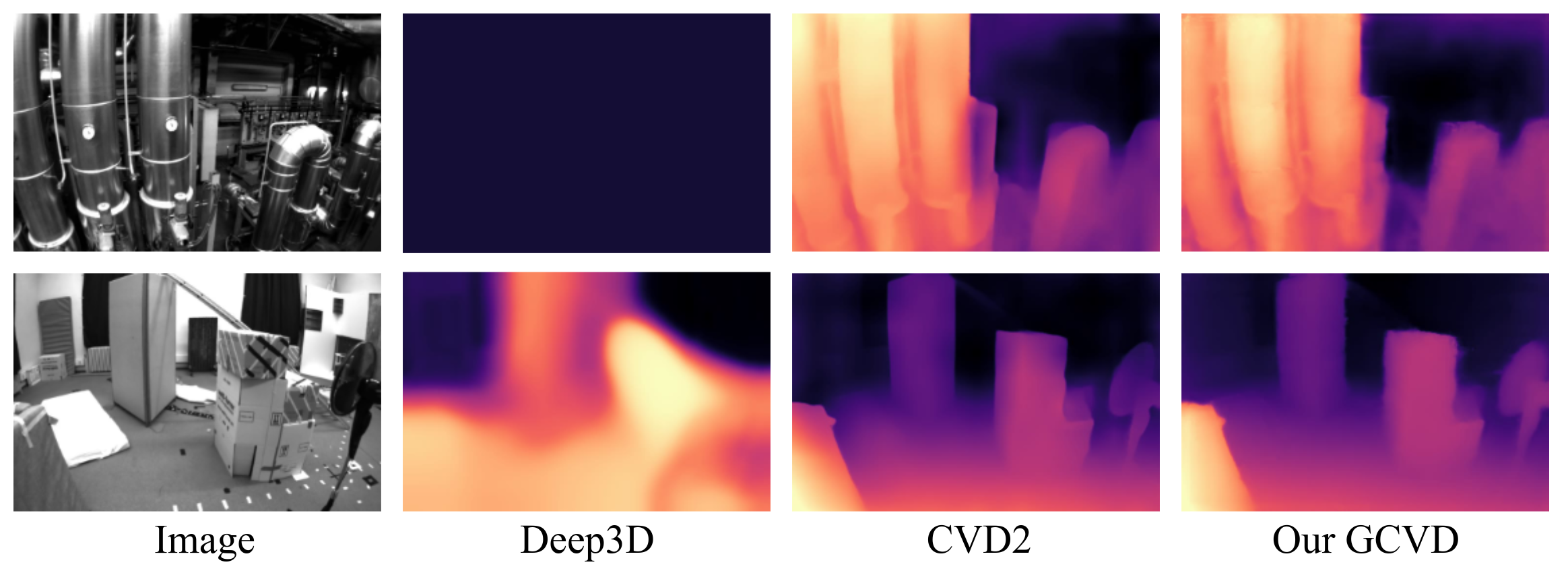
Figure 8: Depth visualization on EuRoC dataset (Burri et al. 2016). CVD2 (Kopf, Rong, and Huang 2021) and our method show plausible depths while Deep3D (Lee et al. 2021) tends to collapse with training from ImageNet pretrained weights.

Table 7: Pose evaluation on EuRoC dataset (Burri et al. 2016). The per-sequence absolute trajectory errors (ATE) are reported in meters.

Sequence	MH	MH	MH	MH	MH	V1	V1	V1	V2	V2	V2	Mean
	01	02	03	04	05	01	02	03	01	02	03
Deep3D	3.24	3.82	2.82	4.26	5.06	1.53	1.57	1.32	1.97	1.87	1.73	2.65
CVD2	1.48	1.32	2.63	4.20	4.31	0.94	1.63	1.19	1.43	1.56	1.74	2.04
Our GCVD	1.33	1.72	1.99	3.78	4.59	1.11	1.07	1.33	0.96	1.88	1.46	1.93

Evaluation on EuRoC (Burri et al. 2016)

The challenging EuRoC dataset (Burri et al. 2016) consists of 11 gray-scale sequences from a stereo camera mounted on a micro aerial vehicle in relatively large indoor environments. The groundtruth camera poses are captured by a laser tracker and motion capture system. We present the absolute trajectory error (ATE) of each sequence in Table 7 and the qualitative comparison of depth estimation in Figure 8. Our method shows the lowest pose error in average. Besides, our GCVD and CVD2 maintain the depth prior of MiDaS while Deep3D produces sub-optimal depth or collapse.

per-frame runtime on a 50-frame video
	Pre-		Main			Post-	Sum
	process.		procedure			process.
Deep3D	1.85		2.27			-	4.13
CVD2	1.73		7.08			5.09	13.90
Ours	0.97		1.40			0.04	2.40
	per-frame	KF	KF	KF association+	non-KF
	pre-process.	decision	optim.	pose graph optim.	optim.
	0.78	0.19	0.33	0.01	1.05

per-frame runtime on a 200-frame video
	Pre-		Main			Post-	Sum
	process.		procedure			process.
Deep3D	1.88		1.14			-	4.13
CVD2	1.61		8.15			5.07	14.83
Ours	0.97		1.53			0.03	2.53
	per-frame	KF	KF	KF association+	non-KF
	pre-process.	decision	optim.	pose graph optim.	optim.
	0.67	0.30	0.29	0.11	1.12

per-frame runtime on a 500-frame video
	Pre-		Main			Post-	Sum
	process.		procedure			process.
Deep3D	1.90		0.85			-	2.75
CVD2	1.60		10.69			5.05	17.34
Ours	1.00		1.71			0.03	2.74
	per-frame	KF	KF	KF association+	non-KF
	pre-process.	decision	optim.	pose graph optim.	optim.
	0.64	0.36	0.35	0.11	1.25

per-frame runtime on a 1000-frame video
	Pre-		Main			Post-	Sum
	process.		procedure			process.
Deep3D	1.91		0.75			-	2.66
CVD2	1.59		15.07			5.07	21.73
Ours	1.03		1.77			0.03	2.83
	per-frame	KF	KF	KF association+	non-KF
	pre-process.	decision	optim.	pose graph optim.	optim.
	0.64	0.39	0.37	0.13	1.28

per-frame runtime on a 2000-frame video
	Pre-		Main			Post-	Sum
	process.		procedure			process.
Deep3D	1.90		0.70			-	2.61
CVD2	1.60		19.44			5.09	26.13
Ours	1.04		1.96			0.03	3.04
	per-frame	KF	KF	KF association+	non-KF
	pre-process.	decision	optim.	pose graph optim.	optim.
	0.63	0.41	0.39	0.25	1.31

Table 8: Runtime comparisons broken down by three main steps. The per-frame runtime are reported in seconds. (KF = keyframe)

Runtime Analysis

We analyze the runtime of each stage in our algorithm in detail. The pipeline is divided into three main steps, pre-processing, main procedure, and post-processing for fair comparison with Deep3D (Lee et al. 2021) and CVD2 (Kopf, Rong, and Huang 2021). The averaged per-frame runtimes of videos of varying length are presented in Table 8. Note that Deep3D does not perform post-processing for video depth and pose estimation.

In the pre-processing step, our method takes fewer time since we only requires adjacent optical flow. In contrast, Deep3D and CVD2 requires multiple pairs of optical flow for a target frame (e.g., $F_{t\pm\gamma\to t},\gamma\in\{1,2,4,8\}$) an thus consumes more time.

In the main procedure for joint depth and pose optimization, although Deep3D takes fewer runtime by reducing the iterations for the optimization of non-first fragments, it may lead to sub-optimal results and yield global inconsistency. On the other hand, CVD2 consumes extremely long time due to the traditional optimization with CPU. The per-frame runtime of our main procedure slightly increase with the longer length of videos mainly due to the geometric verification in keyframe association and increasing non-sequential edges for pose graph optimization. Nevertheless, we emphasize the global consistency, especially in long videos. In the last post-processing step, we re-implement the post-processing proposed by CVD2 with GPU to shorten the computational time.

In sum, the proposed method shows strong efficiency by using keyframe-based pose graph and optimization. Our globally-consistent method is slightly slower than Deep3D for the videos which is greater than 500 frames, yet is able to perform the fastest for the video less than 500 frames.

Limitations

Our method can achieve globally consistent depth and pose estimation with efficient test-time training. Nevertheless, we discuss the following cases that may introduce poor performance.

Restriction by optical flow estimation. Although the dense optical flow estimation can improve the robustness of traditional sparse features, the performance of depth and pose substantially relies on the accurate optical flow. Yet, the state-of-the-art optical flow estimation could still suffer from the generalization issues and thus produce un-satisfied flow estimation in some cases. Furthermore, the forward-backward consistency check is helpful but still cannot fully guarantee the accuracy of optical flow. Hence, how to further improve the dense optical flow estimation remains a promising future direction.

Learnable camera intrinsic parameters. In this work, we assume an ideal camera intrinsic with fixed focal length to simplify the learning of scale consistency in depth and camera pose. It is still challenging on handing the videos with varying focal lengths for global consistency. Thus, we put the reconstruction of varying focal length in our future directions.

References

- Agarwal, Mierle, and Others (2022) Agarwal, S.; Mierle, K.; and Others. 2022. Ceres Solver. http://ceres-solver.org.
- Bao et al. (2019) Bao, W.; Lai, W.-S.; Ma, C.; Zhang, X.; Gao, Z.; and Yang, M.-H. 2019. Depth-aware video frame interpolation. In CVPR.
- Barath et al. (2021) Barath, D.; Mishkin, D.; Eichhardt, I.; Shipachev, I.; and Matas, J. 2021. Efficient Initial Pose-graph Generation for Global SfM. In CVPR.
- Bay, Tuytelaars, and Van Gool (2006) Bay, H.; Tuytelaars, T.; and Van Gool, L. 2006. Surf: Speeded up robust features. In ECCV.
- Bian et al. (2019) Bian, J.; Li, Z.; Wang, N.; Zhan, H.; Shen, C.; Cheng, M.-M.; and Reid, I. 2019. Unsupervised scale-consistent depth and ego-motion learning from monocular video. NeurIPS.
- Bloesch et al. (2018) Bloesch, M.; Czarnowski, J.; Clark, R.; Leutenegger, S.; and Davison, A. J. 2018. CodeSLAM—learning a compact, optimisable representation for dense visual SLAM. In CVPR.
- Burri et al. (2016) Burri, M.; Nikolic, J.; Gohl, P.; Schneider, T.; Rehder, J.; Omari, S.; Achtelik, M. W.; and Siegwart, R. 2016. The EuRoC micro aerial vehicle datasets. The International Journal of Robotics Research (IJRR).
- Casser et al. (2019) Casser, V.; Pirk, S.; Mahjourian, R.; and Angelova, A. 2019. Depth prediction without the sensors: Leveraging structure for unsupervised learning from monocular videos. In AAAI.
- Chen et al. (2016) Chen, W.; Fu, Z.; Yang, D.; and Deng, J. 2016. Single-image depth perception in the wild. NeurIPS.
- Chen et al. (2020) Chen, W.; Qian, S.; Fan, D.; Kojima, N.; Hamilton, M.; and Deng, J. 2020. Oasis: A large-scale dataset for single image 3d in the wild. In CVPR.
- Chen, Schmid, and Sminchisescu (2019) Chen, Y.; Schmid, C.; and Sminchisescu, C. 2019. Self-supervised learning with geometric constraints in monocular video: Connecting flow, depth, and camera. In ICCV.
- Choi et al. (2019) Choi, I.; Gallo, O.; Troccoli, A.; Kim, M. H.; and Kautz, J. 2019. Extreme view synthesis. In CVPR.
- Czarnowski et al. (2020) Czarnowski, J.; Laidlow, T.; Clark, R.; and Davison, A. J. 2020. Deepfactors: Real-time probabilistic dense monocular slam. IEEE Robotics and Automation Letters.
- Du et al. (2020) Du, R.; Turner, E.; Dzitsiuk, M.; Prasso, L.; Duarte, I.; Dourgarian, J.; Afonso, J.; Pascoal, J.; Gladstone, J.; Cruces, N.; Izadi, S.; Kowdle, A.; Tsotsos, K.; and Kim, D. 2020. DepthLab: Real-Time 3D Interaction With Depth Maps for Mobile Augmented Reality. In Proceedings of the 33rd Annual ACM Symposium on User Interface Software and Technology, UIST. ACM.
- Eigen and Fergus (2015) Eigen, D.; and Fergus, R. 2015. Predicting depth, surface normals and semantic labels with a common multi-scale convolutional architecture. In ICCV.
- Eigen, Puhrsch, and Fergus (2014) Eigen, D.; Puhrsch, C.; and Fergus, R. 2014. Depth Map Prediction from a Single Image using a Multi-Scale Deep Network. In NeurIPS. Curran Associates, Inc.
- Engel, Schöps, and Cremers (2014) Engel, J.; Schöps, T.; and Cremers, D. 2014. LSD-SLAM: Large-scale direct monocular SLAM. In ECCV.
- et al. (2017) et al., K. T. 2017. Cnn-slam: Real-time dense monocular slam with learned depth prediction. In CVPR.
- Fischler and Bolles (1981) Fischler, M. A.; and Bolles, R. C. 1981. Random sample consensus: a paradigm for model fitting with applications to image analysis and automated cartography. Communications of the ACM.
- Furukawa and Hernández (2015) Furukawa, Y.; and Hernández, C. 2015. Multi-View Stereo: A Tutorial. Found. Trends. Comput. Graph. Vis.
- Garg et al. (2016) Garg, R.; Bg, V. K.; Carneiro, G.; and Reid, I. 2016. Unsupervised cnn for single view depth estimation: Geometry to the rescue. In ECCV.
- Geiger et al. (2013) Geiger, A.; Lenz, P.; Stiller, C.; and Urtasun, R. 2013. Vision meets Robotics: The KITTI Dataset. International Journal of Robotics Research (IJRR).
- Godard, Mac Aodha, and Brostow (2017) Godard, C.; Mac Aodha, O.; and Brostow, G. J. 2017. Unsupervised monocular depth estimation with left-right consistency. In CVPR.
- Godard et al. (2019) Godard, C.; Mac Aodha, O.; Firman, M.; and Brostow, G. J. 2019. Digging into self-supervised monocular depth estimation. In ICCV.
- Gonzalez and Kim (2021) Gonzalez, J. L.; and Kim, M. 2021. PLADE-Net: Towards Pixel-Level Accuracy for Self-Supervised Single-View Depth Estimation With Neural Positional Encoding and Distilled Matting Loss. In CVPR.
- Gordon et al. (2019) Gordon, A.; Li, H.; Jonschkowski, R.; and Angelova, A. 2019. Depth from videos in the wild: Unsupervised monocular depth learning from unknown cameras. In ICCV.
- Hartley and Zisserman (2003) Hartley, R.; and Zisserman, A. 2003. Multiple view geometry in computer vision. Cambridge university press.
- He et al. (2016) He, K.; Zhang, X.; Ren, S.; and Sun, J. 2016. Deep residual learning for image recognition. In CVPR.
- Holynski and Kopf (2018) Holynski, A.; and Kopf, J. 2018. Fast Depth Densification for Occlusion-aware Augmented Reality. 37(6).
- Huang et al. (2018) Huang, P.-H.; Matzen, K.; Kopf, J.; Ahuja, N.; and Huang, J.-B. 2018. Deepmvs: Learning multi-view stereopsis. In CVPR.
- Im et al. (2019) Im, S.; Jeon, H.-G.; Lin, S.; and Kweon, I. S. 2019. Dpsnet: End-to-end deep plane sweep stereo. arXiv preprint arXiv:1905.00538.
- Jiao, Tran, and Shi (2021) Jiao, Y.; Tran, T. D.; and Shi, G. 2021. EffiScene: Efficient Per-Pixel Rigidity Inference for Unsupervised Joint Learning of Optical Flow, Depth, Camera Pose and Motion Segmentation. In CVPR.
- Jung, Park, and Yoo (2021) Jung, H.; Park, E.; and Yoo, S. 2021. Fine-Grained Semantics-Aware Representation Enhancement for Self-Supervised Monocular Depth Estimation. In ICCV.
- Klein and Murray (2007) Klein, G.; and Murray, D. 2007. Parallel tracking and mapping for small AR workspaces. In 2007 6th IEEE and ACM International Symposium on Mixed and Augmented Reality.
- Kopf, Rong, and Huang (2021) Kopf, J.; Rong, X.; and Huang, J.-B. 2021. Robust consistent video depth estimation. In CVPR.
- Kümmerle et al. (2011) Kümmerle, R.; Grisetti, G.; Strasdat, H.; Konolige, K.; and Burgard, W. 2011. g2o: A general framework for graph optimization. In ICRA.
- Lee et al. (2021) Lee, Y.-C.; Tseng, K.-W.; Chen, Y.-T.; Chen, C.-C.; Chen, C.-S.; and Hung, Y.-P. 2021. 3D Video Stabilization With Depth Estimation by CNN-Based Optimization. In CVPR.
- Li et al. (2019a) Li, S.; Xue, F.; Wang, X.; Yan, Z.; and Zha, H. 2019a. Sequential adversarial learning for self-supervised deep visual odometry. In ICCV.
- Li et al. (2019b) Li, Z.; Dekel, T.; Cole, F.; Tucker, R.; Snavely, N.; Liu, C.; and Freeman, W. T. 2019b. Learning the depths of moving people by watching frozen people. In CVPR.
- Li and Snavely (2018) Li, Z.; and Snavely, N. 2018. Megadepth: Learning single-view depth prediction from internet photos. In CVPR.
- Liu et al. (2021) Liu, A.; Tucker, R.; Jampani, V.; Makadia, A.; Snavely, N.; and Kanazawa, A. 2021. Infinite nature: Perpetual view generation of natural scenes from a single image. In ICCV.
- Liu et al. (2009) Liu, F.; Gleicher, M.; Jin, H.; and Agarwala, A. 2009. Content-preserving warps for 3D video stabilization. ACM TOG.
- Liu et al. (2015) Liu, F.; Shen, C.; Lin, G.; and Reid, I. 2015. Learning depth from single monocular images using deep convolutional neural fields. IEEE TPAMI.
- Long et al. (2021) Long, X.; Liu, L.; Li, W.; Theobalt, C.; and Wang, W. 2021. Multi-view Depth Estimation using Epipolar Spatio-Temporal Networks. In CVPR.
- Long et al. (2020) Long, X.; Liu, L.; Theobalt, C.; and Wang, W. 2020. Occlusion-aware depth estimation with adaptive normal constraints. In ECCV.
- Lowe (2004) Lowe, D. G. 2004. Distinctive image features from scale-invariant keypoints. IJCV.
- Luo et al. (2020) Luo, X.; Huang, J.-B.; Szeliski, R.; Matzen, K.; and Kopf, J. 2020. Consistent video depth estimation. ACM TOG.
- Mayer et al. (2016) Mayer, N.; Ilg, E.; Hausser, P.; Fischer, P.; Cremers, D.; Dosovitskiy, A.; and Brox, T. 2016. A large dataset to train convolutional networks for disparity, optical flow, and scene flow estimation. In CVPR.
- Miangoleh et al. (2021) Miangoleh, S. M. H.; Dille, S.; Mai, L.; Paris, S.; and Aksoy, Y. 2021. Boosting Monocular Depth Estimation Models to High-Resolution via Content-Adaptive Multi-Resolution Merging. In CVPR.
- Moulon et al. (2016) Moulon, P.; Monasse, P.; Perrot, R.; and Marlet, R. 2016. Openmvg: Open multiple view geometry. In International Workshop on Reproducible Research in Pattern Recognition.
- Mur-Artal, Montiel, and Tardos (2015) Mur-Artal, R.; Montiel, J. M. M.; and Tardos, J. D. 2015. ORB-SLAM: a versatile and accurate monocular SLAM system. IEEE Transactions on Robotics.
- Nathan Silberman and Fergus (2012) Nathan Silberman, P. K., Derek Hoiem; and Fergus, R. 2012. Indoor Segmentation and Support Inference from RGBD Images. In ECCV.
- Ranftl et al. (2020) Ranftl, R.; Lasinger, K.; Hafner, D.; Schindler, K.; and Koltun, V. 2020. Towards Robust Monocular Depth Estimation: Mixing Datasets for Zero-shot Cross-dataset Transfer. IEEE TPAMI.
- Ranjan et al. (2019) Ranjan, A.; Jampani, V.; Balles, L.; Kim, K.; Sun, D.; Wulff, J.; and Black, M. J. 2019. Competitive collaboration: Joint unsupervised learning of depth, camera motion, optical flow and motion segmentation. In CVPR.
- Rublee et al. (2011) Rublee, E.; Rabaud, V.; Konolige, K.; and Bradski, G. 2011. ORB: An efficient alternative to SIFT or SURF. In ICCV.
- Saxena, Sun, and Ng (2008) Saxena, A.; Sun, M.; and Ng, A. Y. 2008. Make3d: Learning 3d scene structure from a single still image. IEEE TPAMI.
- Schonberger and Frahm (2016) Schonberger, J. L.; and Frahm, J.-M. 2016. Structure-from-motion revisited. In CVPR.
- Shotton et al. (2013) Shotton, J.; Glocker, B.; Zach, C.; Izadi, S.; Criminisi, A.; and Fitzgibbon, A. 2013. Scene coordinate regression forests for camera relocalization in RGB-D images. In CVPR.
- Sturm et al. (2012) Sturm, J.; Engelhard, N.; Endres, F.; Burgard, W.; and Cremers, D. 2012. A Benchmark for the Evaluation of RGB-D SLAM Systems. In IEEE/RSJ Int. Conf. Intell. Robot. Syst. (IROS).
- Sun et al. (2021) Sun, J.; Xie, Y.; Chen, L.; Zhou, X.; and Bao, H. 2021. NeuralRecon: Real-Time Coherent 3D Reconstruction from Monocular Video. In CVPR.
- Teed and Deng (2019) Teed, Z.; and Deng, J. 2019. DeepV2D: Video to Depth with Differentiable Structure from Motion. In International Conference on Learning Representations.
- Teed and Deng (2020) Teed, Z.; and Deng, J. 2020. Raft: Recurrent all-pairs field transforms for optical flow. In ECCV.
- Teed and Deng (2021) Teed, Z.; and Deng, J. 2021. Droid-slam: Deep visual slam for monocular, stereo, and rgb-d cameras. NeurIPS.
- Triggs et al. (1999) Triggs, B.; McLauchlan, P. F.; Hartley, R. I.; and Fitzgibbon, A. W. 1999. Bundle adjustment—a modern synthesis. In International workshop on vision algorithms. Springer.
- Ummenhofer et al. (2017) Ummenhofer, B.; Zhou, H.; Uhrig, J.; Mayer, N.; Ilg, E.; Dosovitskiy, A.; and Brox, T. 2017. Demon: Depth and motion network for learning monocular stereo. In CVPR.
- Vaswani et al. (2017) Vaswani, A.; Shazeer, N.; Parmar, N.; Uszkoreit, J.; Jones, L.; Gomez, A. N.; Kaiser, Ł.; and Polosukhin, I. 2017. Attention is all you need. In NeurIPS.
- Wang et al. (2021) Wang, J.; Zhong, Y.; Dai, Y.; Birchfield, S.; Zhang, K.; Smolyanskiy, N.; and Li, H. 2021. Deep Two-View Structure-from-Motion Revisited. In CVPR.
- Wang et al. (2004) Wang, Z.; Bovik, A. C.; Sheikh, H. R.; and Simoncelli, E. P. 2004. Image quality assessment: from error visibility to structural similarity. IEEE TIP.
- Watson et al. (2021) Watson, J.; Mac Aodha, O.; Prisacariu, V.; Brostow, G.; and Firman, M. 2021. The Temporal Opportunist: Self-Supervised Multi-Frame Monocular Depth. In CVPR.
- Wei et al. (2020) Wei, X.; Zhang, Y.; Li, Z.; Fu, Y.; and Xue, X. 2020. Deepsfm: Structure from motion via deep bundle adjustment. In ECCV.
- Wimbauer et al. (2021) Wimbauer, F.; Yang, N.; von Stumberg, L.; Zeller, N.; and Cremers, D. 2021. MonoRec: Semi-supervised dense reconstruction in dynamic environments from a single moving camera. In CVPR.
- Wu et al. (2011) Wu, C.; et al. 2011. VisualSFM: A visual structure from motion system.
- Wu et al. (2019) Wu, Y.; Kirillov, A.; Massa, F.; Lo, W.-Y.; and Girshick, R. 2019. Detectron2. https://github.com/facebookresearch/detectron2.
- Wulff et al. (2012) Wulff, J.; Butler, D. J.; Stanley, G. B.; and Black, M. J. 2012. Lessons and insights from creating a synthetic optical flow benchmark. In ECCV Workshop on Unsolved Problems in Optical Flow and Stereo Estimation.
- Yao et al. (2018) Yao, Y.; Luo, Z.; Li, S.; Fang, T.; and Quan, L. 2018. Mvsnet: Depth inference for unstructured multi-view stereo. In ECCV.
- Yin et al. (2021) Yin, W.; Zhang, J.; Wang, O.; Niklaus, S.; Mai, L.; Chen, S.; and Shen, C. 2021. Learning to recover 3d scene shape from a single image. In CVPR.
- Yin and Shi (2018) Yin, Z.; and Shi, J. 2018. Geonet: Unsupervised learning of dense depth, optical flow and camera pose. In CVPR.
- Yoon et al. (2020) Yoon, J. S.; Kim, K.; Gallo, O.; Park, H. S.; and Kautz, J. 2020. Novel view synthesis of dynamic scenes with globally coherent depths from a monocular camera. In CVPR.
- Zhang and Scaramuzza (2018) Zhang, Z.; and Scaramuzza, D. 2018. A Tutorial on Quantitative Trajectory Evaluation for Visual(-Inertial) Odometry. In IEEE/RSJ Int. Conf. Intell. Robot. Syst. (IROS).
- Zhou, Ummenhofer, and Brox (2018) Zhou, H.; Ummenhofer, B.; and Brox, T. 2018. Deeptam: Deep tracking and mapping. In ECCV.
- Zhou et al. (2017) Zhou, T.; Brown, M.; Snavely, N.; and Lowe, D. G. 2017. Unsupervised learning of depth and ego-motion from video. In CVPR.
- Zhou et al. (2021) Zhou, Z.; Fan, X.; Shi, P.; and Xin, Y. 2021. R-MSFM: Recurrent Multi-Scale Feature Modulation for Monocular Depth Estimating. In ICCV.
- Zou et al. (2020) Zou, Y.; Ji, P.; Tran, Q.-H.; Huang, J.-B.; and Chandraker, M. 2020. Learning monocular visual odometry via self-supervised long-term modeling. In ECCV.