Non-destructive one-shot device testing under step-stress model with Weibull lifetime distributions

Abstract

One-shot devices are product or equipment that can be used only once, so they get destroyed when tested. However, the destructiveness assumption may not be necessary in many practical applications such as assessing the effect of temperature on some electronic components, yielding to the so called non-destructive one-shot devices. Further, one-shot devices generally have large mean lifetime to failure, and so accelerated life tests (ALTs) must be performed for inference. The step-stress ALT shorten the lifetime of the products by increasing the stress level at which units are subjected to progressively at pre-specified times. Then, the non-destructive devices are tested at certain inspection times and surviving units can continue within the experiment providing extra information. Classical estimation methods based on the maximum likelihood estimator (MLE) enjoy suitable asymptotic properties but they lack of robustness. In this paper, we develop robust inferential methods for non-destructive one-shot devices based on the popular density power divergence (DPD) for estimating and testing under the step-stress model with Weibull lifetime distributions. We theoretically and empirically examine the asymptotic and robustness properties of the minimum DPD estimators and Wald-type test statistics based on them. Moreover, we develop robust estimators and confidence intervals for some important lifetime characteristics, namely reliability at certain mission times, distribution quantiles and mean lifetime of a device. Finally, we analyze the effect of temperature in three electronic components, solar lights, medium power silicon bipolar transistors and LED lights using real data arising from an step-stress ALT.

1 Introduction

One-shot device tests involve an extreme case of interval censoring, wherein we only know if a device has failed or not when it is tested. Frequently, such products have large mean times to failure under normal operating conditions and hence accelerated life tests (ALTs), in which the life of the products is shortened by increasing the stress level at which the devices are subjected to, are commonly used to infer their lifetime distribution. The objective of these tests is to induce the devices to fail in a shorter time, so as to efficiently collect useful and sufficient information for modelling and analyzing the lifetimes of the products, depending on the stress level. After suitable inference is developed, we can extrapolate the results to normal operating conditions; see Meeter and Mecker (1994) and Meeker et al. (1998). This way, some lifetime characteristics of interest, such as reliability of the device at certain mission times, distribution quantiles or mean lifetime of the product, may be estimated.

Accelerated life-testing may be performed either at constant high stress level or linearly increasing stress levels, step-by-step over time. The multiple step-stress ALT increases the stress level at which devices are tested at pre-specified times, referred so as times of stress change. Step-stress ALTs require less samples and are more efficient and less expensive to collect lifetime data than constant-stress ALTs. Clearly, a model relating the effect of increased stress levels on the lifetime distribution of a device is needed. Three main proposals have been made in the literature: tampered random variable model (DeGroot and Goel (1979)), tampered failure-rate model (Bhattacharyya and Soejoeti (1989)), and cumulative exposure model Nelson (1980). We will adopt the cumulative exposure approach here, which relates the lifetime distribution of experimental devices at one stress level to the distributions at preceding stress levels by assuming that the residual life of the experimental devices depends only on the current cumulative exposure experienced and current stress, with no memory of how the exposure was accumulated. Therefore, the lifetime of surviving devices is modelled by to the cumulative distribution for the current stress, but adjusted by the cumulative exposure experienced so far.

Balakrishnan (2009) has reviewed inferential techniques for step-stress models and associated optimal accelerated life-tests, based on complete and censored samples. In the present work, we will assume that lifetimes of devices follow a Weibull distribution, with common shape parameter (not depending on the stress level), and scale parameter related to the current stress level through a log-linear relationship. Weibull distribution is commonly used as a lifetime model in engineering, physical and biomedical sciences. Further, by assuming common shape, it can be parameterized as a proportional hazards model, meaning that the hazard rates of any two products stay constant over time. In an accelerated life testing application, a common assumption is that the ALT does not change the failure mode of the units or materials, and so the homogeneity condition on the shape is valid in most applications and the stress level changes only the scale parameter of the life distribution. However, the homogeneity condition on the shape parameter may be violated in some practical applications, when the stress level may affect the shape parameter as well.

Destructive one-shot devices, which get destroyed when tested, have been widely studied in the literature. The data collected from such devices are either left- or right-censored, with the lifetime being less than the inspection time if the device fails when tested (resulting in left-censoring), and the lifetime being more than the inspection time for surviving devices (resulting in right-censoring). However, the destructiveness assumption may not be appropriate in some engineering applications, and so the surviving devices would continue in the experiment, providing extra-information. The proposed model would also be useful for experiments wherein the exact failure times of devices can not be recorded, but the state of the devices can only be checked at certain readout times. For example, Gouno (2001) used this experimental set up to infer the lifetime distribution of two electronic products related to medium-power silicon bipolar transistors.

Constant-stress ALT for one-shot devices have been studied extensively. Fan et al. (2009) compared three different priors in the Bayesian approach for making predictions on the reliability and the mean lifetime of electro-explosive devices at normal operating conditions under the exponential lifetime distribution, and Cai et al. (2011) suggested a Bayesian proportional hazards model for analyzing the uterine fibroid data from an epidemiological study. Balakrishnan and Ling (2012, 2013) developed an Expectation-Maximization (EM) algorithm for one-shot device accelerated life testing with exponential and Weibull lifetimes, and Ling et al. (2015) subsequently extended the techniques to general proportional hazards models. Likewise, Balakrishnan and Ling (2014) proposed optimal design plans with multiple stress factors for one-shot device testing under a Weibull distribution. Some other lifetime distributions such as Lindey, Gamma or log-normal have been similarly considered.

In contrast, little attention has been paid to step-stress ALT for one-shot devices. Ling (2018) proposed optimal design for simple step-stress ALTs for one-shot devices under exponential distribution, and Ling and Hu (2020) extended the theory to Weibull distribution lifetimes. One may refer to the recent book by Balakrishnan et al. (2021) for a detailed state-of-the-art review on inferential techniques for ALTs with one-shot devices.

Recent works on one-shot devices have shown the advantage of using divergence-based methods in terms of robustness, with an unavoidable (but not significant) loss of efficiency. Balakrishnan et al. (2019, 2020a, 2020b, 2021) developed robust estimation methods based on density power divergence (DPD) for the constant-stress model and then constructed robust test statistics for testing composite null hypothesis for different lifetime distributions, including exponential and Weibull. Recently, Castilla et al. (2022) developed robust estimators and test statistics based on the DPD for non-destructive one-shot devices tested under multiple step-stress ALT under exponential lifetimes, obtaining good empirical results. In this paper, we extend thiss work for the case of Weibull lifetime distributions.

The rest of this paper is organised as follows. Section 3 presents the multiple step-stress model for Weibull lifetime distributions. In Section 4, the classical maximum likelihood estimator (MLE) of the model and the minimum DPD estimators (MDPDE) are introduced, and their estimating equations and asymptotic properties are discussed. Section 5 investigates several lifetime characteristics, namely, reliability, distribution quantiles and mean lifetime, as well as their point estimation and confidence intervals (CIs) based on the MDPDEs. Further, transformed CIs are proposed to avoid some practical drawback of direct CIs. In Section 6, Wald-type test statistics, based on the MDPDE, for testing general composite null hypothesis are developed. Asymptotic distribution of the proposed test statistic under the null hypothesis and asymptotic behaviour of the power of the test are established. Section 7 theoretically study the robustness properties of the estimators and test statistics based on the MDPDE through the analysis of their influence function (IF). In Section 9, an extensive simulation study is carried out for examining the robustness properties of the estimators and the test statistics is carried out. Section 10 illustrates the applicability of the proposed model and the inferential methods developed here with three real datasets from the reliability literature, regarding the effect of temperature in different electronic components. Finally, some concluding remarks are made in Section 11.

2 Motivating Data Sets

We aim to analyze the influence of temperature in some electronic components such as solar lights, medium power silicon bipolar transistors and LED lights. Allowing systems to run for prolonged periods of time in high temperatures can severely decrease the longevity and reliability of some electronic devices. Therefore, in order to get the most out of an electronic component in different environments or otherwise choose the best material for a certain function, it will be interest to study its reliability based on the temperature. Recall that the step-stress model enables to obtain more accurate estimates with fewer sample sizes than constant-stress ALTs. Therefore, the model is especially accurate for the presented industrial experiments, which traditionally have small sample sizes.

2.1 Effect of temperature on solar lighting devices

Solar lights are known to be resilient and environmental-friendly by design and so they offer an attractive lighting alternative for outdoor and indoor places. Conversely, there is an unwanted effect of extreme weather on the reliability of such devices. In particular, the efficiency of solar lights generally decreases as the temperature rises, due to a voltage decrease. Under normal operating conditions, solar lighting devices are expected to last for hundreds of hours, and therefore an ALT must be carried out to infer the effect of temperature on solar lighting devices. For this purpose, Han and Kundu (2014) conducted a simple step-stress accelerated life testing experiment. A set of 35 solar light prototypes were placed on equal environmental conditions, and the temperature was increased at a pre-specified time $\tau_{1}=5$ (in hundred hours) from normal operating temperature ($293K$) to $353K.$ The experiment was terminated at $\tau_{2}=6$ (in hundred hours), when only $4$ devices were still functioning. Failure times observed during the experiment are as follows:

10.14, 0.783, 1.324, 1.582, 1.716, 1.794, 1.883, 2.293, 2.660, 2.674, 2.725, 3.085, 3.924, 4.396, 4.612, 4.892, 5.002, 5.022, 5.082, 5.112, 5.147, 5.238, 5.244, 5.247, 5.305, 5.337, 5.407, 5.408, 5.445, 5.483, 5.717.

The collected data can be easily transformed into non-destructive one-shot devices with inspection times $t=1.5,3,5,5.2,5.4,6$ (in hundred ours). Further, we can assume that the lifetime of solar light follows a Weibull distribution and that its scale parameter depends on the surrounding temperature.

2.2 Effect of temperature on medium power silicon bipolar transistors

Gouno (2001) carried out a temperature multiple step-stress ALT with 31 medium power silicon bipolar transistors. He considered the Arrhenius model with censored data to describe the temperature stress. The devices were successively exposed to 10 temperature levels of 120, 140, 160, 180, 190, 200, 210, 220, 230, 240 degrees during equal time intervals of length 168 h. At each time of stress change, the number of failures were recorded, yielding the observed vector of failures to be $n=(0,0,0,2,5,5,3,3,0,9).$ Here, all right-censored data have been removed from the dataset. We will assume that the lifetime of the medium power silicon bipolar transistors follows a Weibull distribution with common shape parameter, and that the Weibull scale parameter is affected by the temperature.

2.3 Effect of temperature on Light Emitting Diodes (LEDs)

Temperature has a tangible effect on the material and output of an LED light. Cold environments favour good functioning of LEDs, and light output diminishes with temperature increment. Zhao and Elsayed (2005) examined the effect of temperature in LEDs though a multiple step-stress ALT experiment with four levels. The LEDs are considered to be working properly as long as the change in the light intensity does not exceed a pre-fixed threshold level. Then, they placed $27$ LED units in a temperature and humidity chamber and the humidity and current in the circuit were held constant at 70% RH and 28 mA, respectively. Four temperature levels were considered during the test, According to expert engineering judgment, temperatures less than $80^{\circ}C$ are not appropriate since it is difficult to observe the LED failure in a reasonable test time. Conversely, temperatures above and above $200^{\circ}C$ are not recommended either as extrapolation can not be justified. Therefore, four temperatures levels ranging from $80$ to $200^{\circ}$ were considered for the ALT as $T=363K,413K,433K$ and $448K.$ The normal operating temperature for LEDs is $50^{\circ}C.$ The times of stress change were fixed at $t=300,500$ and $600$ hours, and the test got terminated at $t=720$ hours. Recorded failure times were as follows:

347, 397, 432, 491, 512, 567, 574, 588, 597, 603, 605, 615, 633, 634, 637, 644, 653, 675, 684, 699, 706, 718, 720.

We will transformed the data to non-destructive one-shot device data in which the inspection times coincide with the times of stress change and further we will assume Weibull lifetime distributions for the LEDs.

3 The multiple step-stress model

We consider the multiple step-stress ALT for one-shot devices with $k$ ordered stress levels $x_{1}<x_{2}<\dots<x_{k}$ and $N$ devices under test. At the start of the experiment, all devices are subjected to the same stress level, $x_{1},$ which gets increased to $x_{2}$ at a certain pre-specified time of stress change, $\tau_{1}.$ All devices are subjected to the new stress level until the next time of stress change, $\tau_{2},$ and the process is repeated until all remaining surviving devices are subjected $k$-th stress, $x_{k}.$ The termination time of the experiment is fixed at $\tau_{k}.$ In addition, we consider $L$ pre-fixed inspection times,

$$0<t_{1}<\dots<t_{l_{1}}=\tau_{1}<t_{l_{1}+1}<\dots<t_{l_{k}}=\tau_{k},$$

where $l_{i}$ denotes the number of inspection times before the $i$-th time of stress change and $l_{k}=L,$ when all the surviving devices are tested and the number of failures is recorded. We assume that all times of stress change are inspection times. The non-destructive assumption implies that all devices that did not fail until a certain time can continue on the experiment.

The cumulative exposure (CE) model forms a composite failure distribution function by assuming that the product lifetime is shifted at the time of stress change such that the survival functions of the change time are the same under two different stress levels. We will assume that the lifetime of devices at a constant stress level $x_{i}$ follow a Weibull distribution with common shape parameter $\eta>0$ (homogeneity condition) and scale parameter $\alpha_{i}>0$ depending on the stress level through the log-linear relationship

$$\alpha_{i}(\boldsymbol{\theta})=\exp(a_{0}+a_{1}x_{i}),\hskip 8.5359pti=1,..,k,$$ (1)

where $\boldsymbol{\theta}=(a_{0},a_{1},\eta)^{T}\in\Theta=\mathbb{R}\times\mathbb{R}^{-}\times\mathbb{R}^{+}.$ Note that the CE assumes that the probability of failure gets increased when the stress level increases, so that the parameter $\theta_{1}$ should be negative. Then, the cumulative distribution function (cdf) of failure time is given by

$$G_{T}(t)=\begin{cases}G_{1}(t)=1-\exp\left(-\left(\frac{t}{\alpha_{1}}\right)^{\eta}\right),&0<t<\tau_{1}\\ G_{2}\left(t+h_{1}\right)=1-\exp\left(-\left(\frac{t+h_{1}}{\alpha_{2}}\right)^{\eta}\right),&\tau_{1}\leq t<\tau_{2},\\ \vdots&\vdots\\ G_{k}\left(t+h_{k-1}\right)=1-\exp\left(-\left(\frac{t+h_{k-1}}{\alpha_{k}}\right)^{\eta}\right),&\tau_{k-1}\leq t<\infty\\ \end{cases},$$ (2)

and correspondingly the reliability function is given by

$$R_{T}(t)=1-G_{T}(t)=\begin{cases}R_{1}(t)=\exp\left(-\left(\frac{t}{\alpha_{1}}\right)^{\eta}\right),&0<t<\tau_{1}\\ R_{2}(t+h_{1})=\exp\left(-\left(\frac{t+h_{1}}{\alpha_{2}}\right)^{\eta}\right),&\tau_{1}\leq t<\tau_{2}\\ \vdots&\vdots\\ R_{K}(t+h_{k-1})=\exp\left(-\left(\frac{t+h_{k-1}}{\alpha_{k}}\right)^{\eta}\right),&\tau_{k-1}\leq t<\infty\\ \end{cases},$$

and the probability distribution function (pdf) is given by

$$g_{T}(t)=\begin{cases}g_{1}(t)=\frac{\eta}{\alpha_{1}}\left(\frac{t}{\alpha_{1}}\right)^{\eta-1}\exp\left(-\left(\frac{t}{\alpha_{1}}\right)^{\eta}\right),&0<t<\tau_{1}\\ g_{2}\left(t+h_{1}\right)=\frac{\eta}{\alpha_{2}}\left(\frac{t+h_{1}}{\alpha_{2}}\right)^{\eta-1}\exp\left(-\left(\frac{t+h_{1}}{\alpha_{2}}\right)^{\eta}\right),&\tau_{1}\leq t<\tau_{2}\\ \vdots&\vdots\\ g_{k}\left(t+h_{k-1}\right)=\frac{\eta}{\alpha_{k}}\left(\frac{t+h_{k-1}}{\alpha_{k}}\right)^{\eta-1}\exp\left(-\left(\frac{t+h_{k-1}}{\alpha_{k}}\right)^{\eta}\right),&\tau_{k-1}\leq t<\infty\\ \end{cases},$$ (3)

with

$$h_{i}=\alpha_{i+1}\sum_{k=0}^{i-1}\left(-\frac{1}{\alpha_{i+1-k}}+\frac{1}{\alpha_{i-k}}\right)\tau_{i-k},$$ (4)

for $i=1,...,k-1.$ Although the distribution function is continuous in $(0,\infty),$ the density function has $k$ points of discontinuity at each time of stress change. Further, the probability of failure at the $j$-th interval is

$$\pi_{j}(\boldsymbol{\theta})=G_{T}(t_{j})-G_{T}(t_{j-1}),\hskip 8.5359ptj=1,..,L,$$ (5)

and finally the probability of survival at the end of the experiment is given by $\pi_{L+1}(\boldsymbol{\theta})=1-G_{T}(t_{L}).$

4 Minimum density power divergence estimator

In this section, we develop robust estimators for the SSALT model under Weibull lifetimes based on the DPD introduced by Basu et al. (1998), and then study their asymptotic and robustness properties.

Let $n_{j}$ denote the number of failures within the $j$-th interval and $n_{L+1}$ denote the number of surviving devices at the end of the experiment. We introduce probability vector $\boldsymbol{\pi}(\boldsymbol{\theta})=(\pi_{1}(\boldsymbol{\theta})),...,\pi_{L+1}(\boldsymbol{\theta}))^{T}$ quantifying the probability of failure within each interval and its corresponding empirical probability vector $\widehat{\boldsymbol{p}}=\left(n_{1}/N,...,n_{L+1}/N\right)^{T}.$ Then, the likelihood function of the multinomial model with probability $\boldsymbol{\pi}(\boldsymbol{\theta})$ and $N$ trials (total number devices tested) is given by

$$\mathcal{L}(\boldsymbol{\theta};n_{1},..,n_{L+1})=\frac{N!}{n_{1}!\cdots n_{L+1}!}\prod_{j=1}^{L+1}\pi_{j}(\boldsymbol{\theta})^{n_{j}}$$

and then the MLE of the model parameter $\boldsymbol{\theta}$ for the SSALT model under Weibull lifetimes is given by

$$\boldsymbol{\widehat{\theta}}^{MLE}=\left(\widehat{a}_{0}^{MLE},\widehat{a}_{1}^{MLE},\widehat{\eta}^{MLE}\right)^{T}=\operatorname{arg}\operatorname{max}_{\boldsymbol{\theta}\in\Theta}\mathcal{L}(\boldsymbol{\theta};n_{1},..,n_{L+1}).$$

It is useful to note that the MLE can be equivalently derived from an information theory approach by using the Kullback-Leibler (KL) divergence between the empirical vector $\widehat{\boldsymbol{p}}$ and the theoretical probability $\boldsymbol{\pi}(\boldsymbol{\theta})$ of the multinomial model, since the expression of the KL divergence is related to the likelihood function as

$$d_{KL}(\boldsymbol{\widehat{p}},\boldsymbol{\pi}(\boldsymbol{\theta}))=\sum_{j=1}^{L+1}\widehat{p}_{j}\log\left(\frac{\widehat{p}_{j}}{\pi_{j}(\boldsymbol{\theta})}\right)=\sum_{i=1}^{L+1}\widehat{p}_{i}\log(\widehat{p}_{i})-\frac{1}{N}\log\mathcal{L}(\boldsymbol{\theta};n_{1},..,n_{L+1}).$$

Then, the minimizer of the KL divergence coincides with the MLE. This classical estimator is known to be asymptotically efficient in the absence of contamination, but it lacks robustness as contamination in the data could influence the parameter estimate. To overcome this, we introduce a family of estimators based on the DPD, indexed by a tuning parameter $\beta\geq 0$ controlling the trade-off between efficiency and robustness.

The DPD between the empirical and theoretical probability vectors, $\widehat{\boldsymbol{p}}$ and $\boldsymbol{\pi},$ is given by

$$d_{\beta}\left(\widehat{\boldsymbol{p}},\boldsymbol{\pi}\left(\boldsymbol{\theta}\right)\right)=\sum_{j=1}^{L+1}\left(\pi_{j}(\boldsymbol{\theta})^{1+\beta}-\left(1+\frac{1}{\beta}\right)\widehat{p}_{j}\pi_{j}(\boldsymbol{\theta})^{\beta}+\frac{1}{\beta}\widehat{p}_{j}^{\beta+1}\right)$$ (6)

and correspondingly the minimum DPD estimator (MDPPE), for $\beta>0,$ is defined as

$$\boldsymbol{\widehat{\theta}}^{\beta}=\left(\widehat{a}_{0}^{\beta},\widehat{a}_{1}^{\beta},\widehat{\eta}^{\beta}\right)^{T}=\operatorname{arg}\operatorname{min}_{\boldsymbol{\theta}\in\Theta}d_{\beta}\left(\widehat{\boldsymbol{p}},\boldsymbol{\pi}\left(\boldsymbol{\theta}\right)\right).$$ (7)

For $\beta=0,$ the DPD can be defined by taking continuos limits $\beta\rightarrow 0,$ and the resulting expression is indeed the KL divergence. Thus, the DPD family generalizes the likelihood procedure to a broader class of estimators, including the classical MLE for the case when $\beta=0.$

The following result establishes the estimating equations of the MDPDE for any $\beta\geq 0.$

Result 1

The estimating equations of the MDPDE for the SSALT model under Weibull lifetime distributions, satisfying the log-linear relation in (1), are given by

$$\boldsymbol{W}^{T}\boldsymbol{D}_{\boldsymbol{\pi}(\boldsymbol{\theta})}^{\beta-1}\left(\widehat{\boldsymbol{p}}-\boldsymbol{\pi}(\boldsymbol{\theta})\right)=\boldsymbol{0}_{3},$$

where $\boldsymbol{0}_{3}$ is the 3-dimensional null vector, $\boldsymbol{D}_{\boldsymbol{\pi}(\boldsymbol{\theta})}$ denotes a $(L+1)\times(L+1)$ diagonal matrix with diagonal entries $\pi_{j}(\boldsymbol{\theta}),$ $j=1,...,L+1,$ and $\boldsymbol{W}$ is a $(L+1)\times 3$ matrix with rows $\boldsymbol{w}_{j}=\boldsymbol{z}_{j}-\boldsymbol{z}_{j-1},$ where

$$\boldsymbol{z}_{j} =g_{T}(t_{j})\begin{pmatrix}-(t_{j}+h_{i-1})\\ -(t_{j}+h_{i-1})x_{i}+h_{i-1}^{\ast}\\ \log\left(\frac{t_{j}+h_{i-1}}{\alpha_{i}}\right)\frac{t_{j}+h_{i-1}}{\eta}\end{pmatrix},\hskip 8.5359ptj=1,...,L$$ (8)

$$h_{i}^{\ast} =h_{i}x_{i+1}+\alpha_{i+1}\sum_{k=0}^{i-1}\left(\frac{x_{i+1-k}}{\alpha_{i+1-k}}-\frac{x_{i-k}}{\alpha_{i-k}}\right)\tau_{i-k},\hskip 8.5359pti=1,..,k-1$$ (9)

with $\boldsymbol{z}_{-1}=\boldsymbol{z}_{L+1}=\boldsymbol{0}$ and $i$ being the stress level at which the units are tested before the $j-$th inspection time.

Proof. See Appendix.                                                                                                              

Note that estimating equations of the MLE are obtained ready by evaluating the previous expression at $\beta=0,$ resulting in

$$\boldsymbol{W}^{T}\boldsymbol{D}_{\boldsymbol{\pi}(\boldsymbol{\theta})}^{-1}\left(\widehat{\boldsymbol{p}}-\boldsymbol{\pi}(\boldsymbol{\theta})\right)=\boldsymbol{0}_{3}.$$

Next, we present the asymptotic distribution of the proposed estimator for any $\beta\geq 0$.

Result 2

Let $\boldsymbol{\theta}_{0}$ be the true value of the parameter $\boldsymbol{\theta}$. Then, the asymptotic distribution of the MDPDE, $\boldsymbol{\widehat{\theta}}^{\beta},$ for the SSALT model, under Weibull lifetime distribution, is given by

$$\sqrt{N}\left(\boldsymbol{\widehat{\theta}}^{\beta}-\boldsymbol{\theta}_{0}\right)\rightarrow\mathcal{N}\left(\boldsymbol{0},\boldsymbol{J}_{\beta}^{-1}(\boldsymbol{\theta}_{0})\boldsymbol{K}_{\beta}(\boldsymbol{\theta}_{0})\boldsymbol{J}_{\beta}^{-1}(\boldsymbol{\theta}_{0})\right),$$

where

$$\boldsymbol{J}_{\beta}(\boldsymbol{\theta}_{0})=\boldsymbol{W}^{T}D_{\boldsymbol{\pi}(\boldsymbol{\theta_{0}})}^{\beta-1}\boldsymbol{W},\hskip 8.5359pt\hskip 8.5359pt\boldsymbol{K}_{\beta}(\boldsymbol{\theta}_{0})=\boldsymbol{W}^{T}\left(D_{\boldsymbol{\pi}(\boldsymbol{\theta_{0}})}^{2\beta-1}-\boldsymbol{\pi}(\boldsymbol{\theta}_{0})^{\beta}\boldsymbol{\pi}(\boldsymbol{\theta}_{0})^{\beta T}\right)\boldsymbol{W},$$ (10)

$D_{\boldsymbol{\pi}(\boldsymbol{\theta_{0}})}$ denotes the diagonal matrix with entries $\pi_{j}(\boldsymbol{\theta_{0}}),$ $j=1,...,L+1,$ and $\boldsymbol{\pi}(\boldsymbol{\theta}_{0})^{\beta}$ denotes the vector with components $\pi_{j}(\boldsymbol{\theta}_{0})^{\beta}.$

Proof. The proof is similar to that of Theorem 2 in Balakrishnan et al. (2022).                                                                                                               The Fisher information matrix associated with the SSALT model under Weibull lifetime distribution is given by $\boldsymbol{I}_{F}(\boldsymbol{\theta}_{0})=\boldsymbol{W}^{T}D_{\boldsymbol{\pi}(\boldsymbol{\theta_{0}})}^{-1}\boldsymbol{W},$ and so the convergence of the MLE is obtained as a particular case at $\beta=0,$ to be

$$\sqrt{N}\left(\boldsymbol{\widehat{\theta}}^{0}-\boldsymbol{\theta}_{0}\right)\rightarrow\mathcal{N}\left(\boldsymbol{0},\boldsymbol{I}_{F}^{-1}(\boldsymbol{\theta}_{0})\right).$$

5 Point estimation and confidence intervals of reliability, distribution quantiles and mean lifetime of a device

Engineering applications often demand estimated values of some important lifetime characteristics, such as the reliability function, distribution quantiles and mean lifetime of a device under normal operating conditions. Hence, point estimation and confidence intervals (CIs) of such lifetime characteristics will be of great interest for reliability engineers. In this section, we develop point estimation and CIs for these three main lifetime characteristics based on the MDPDEs. Further, we establish asymptotic distributions of each lifetime characteristic and derive the corresponding approximate direct and transformed CIs.

Lifetime distribution characteristics are functions of the model parameter $\boldsymbol{\theta},$ and so their asymptotic distribution can be derived by using the Delta-method. In particular, the reliability of the device at a constant stress level, $x_{0},$ and at a fixed time $t,$ is given by

$$R_{t}(\boldsymbol{\theta})=\exp\left(-\left(\frac{t}{\exp(a_{0}+a_{1}x_{0})}\right)^{\eta}\right),$$ (11)

the $1-\alpha$ distribution quantile at stress level $x_{0}$ is given by the inverse distribution (or reliability) function, as

$$Q_{1-\alpha}(\boldsymbol{\theta})=R_{0}^{-1}(1-\alpha)=G_{0}^{-1}(\alpha)=\exp(a_{0}+a_{1}x_{0})\left(-\log(1-\alpha)\right)^{\frac{1}{\eta}},$$ (12)

and the mean lifetime of the device is given by

$$\operatorname{E}_{T}(\boldsymbol{\theta})=\mathbb{E}_{\boldsymbol{\theta}}[T]=\exp(a_{0}+a_{1}x_{0})\Gamma\left(1+\frac{1}{\eta}\right)$$ (13)

with $\Gamma(\cdot)$ denoting the gamma function.

Given an MDPDE, $\widehat{\boldsymbol{\theta}}^{\beta}$, its is straightforward to obtain a point estimation of the reliability at a certain time, quantile and mean lifetime of devices under normal operating conditions by substituting the estimated parameters in (11), (12) and (13), respectively. The next result presents the asymptotic distributions of these three estimated lifetime characteristics based on the MDPDE.

Result 3

Let $\boldsymbol{\theta}_{0}$ be the true value of the parameter $\boldsymbol{\theta},$ and then consider $\widehat{\boldsymbol{\theta}}^{\beta}$ as the MDPDE with tuning parameter $\beta.$ Then, the asymptotic distribution of the estimated reliability of devices at a certain time $t$ under normal operating conditions, based on the MDPDE, $R_{t}(\widehat{\boldsymbol{\theta}}^{\beta}),$ is given by

$$\sqrt{N}(R_{t}(\widehat{\boldsymbol{\theta}}^{\beta})-R_{t}(\boldsymbol{\theta}_{0}))\xrightarrow[N\rightarrow\infty]{L}\mathcal{N}\left(\boldsymbol{0},\sigma(R_{t}(\boldsymbol{\theta}_{0}))\right)$$

with

$$\sigma(R_{0}^{\beta}(t))^{2}=\nabla R_{t}\left(\boldsymbol{\theta}_{0}\right)^{T}\boldsymbol{J}_{\beta}^{-1}(\boldsymbol{\theta}_{0})\boldsymbol{K}_{\beta}(\boldsymbol{\theta}_{0})\boldsymbol{J}_{\beta}^{-1}(\boldsymbol{\theta}_{0})\nabla R_{t}\left(\boldsymbol{\theta}_{0}\right),$$

where the matrices $\boldsymbol{J}_{\beta}(\boldsymbol{\theta}_{0})$ and $\boldsymbol{K}_{\beta}(\boldsymbol{\theta}_{0})$ are as defined in (10) and $\nabla R_{t}\left(\boldsymbol{\theta}\right)^{T}=tg_{0}(t)\left(1,x_{0},-\log\left(\frac{t}{\alpha_{0}}\right)\frac{1}{\eta}\right)$ is the gradient of the function $R_{t}(\boldsymbol{\theta})$ defined in (11).

Result 4

Under the same assumptions as in Result 4, the asymptotic distribution of the estimated $1-\alpha$ quantile of the lifetime distribution of devices under normal operating conditions based on the MDPDE, $Q_{1-\alpha}(\widehat{\boldsymbol{\theta}}^{\beta}),$ is given by

$$\sqrt{N}(\widehat{Q}_{1-\alpha}(\widehat{\boldsymbol{\theta}}^{\beta})-Q_{1-\alpha}(\boldsymbol{\theta}_{0}))\xrightarrow[N\rightarrow\infty]{L}\mathcal{N}\left(\boldsymbol{0},\sigma(Q_{1-\alpha}(\boldsymbol{\theta}_{0}))\right)$$

with

$$\sigma(Q_{1-\alpha}(\boldsymbol{\theta}_{0}))^{2}=\nabla Q_{1-\alpha}\left(\boldsymbol{\theta}_{0}\right)^{T}\boldsymbol{J}_{\beta}^{-1}(\boldsymbol{\theta}_{0})\boldsymbol{K}_{\beta}(\boldsymbol{\theta}_{0})\boldsymbol{J}_{\beta}^{-1}(\boldsymbol{\theta}_{0})\nabla Q_{1-\alpha}\left(\boldsymbol{\theta}_{0}\right)$$

where the matrices $\boldsymbol{J}_{\beta}(\boldsymbol{\theta}_{0})$ and $\boldsymbol{K}_{\beta}(\boldsymbol{\theta}_{0})$ are as defined in (10) and $\nabla Q_{1-\alpha}(\boldsymbol{\theta})^{T}=Q_{1-\alpha}(\boldsymbol{\theta})\left(1,x_{0},\frac{-\log(-\log(1-\alpha))}{\eta^{2}}\right)$ is the gradient of the function $Q_{1-\alpha}(\boldsymbol{\theta})$ defined in (12).

Result 5

Under the same assumptions as in Result 3, the asymptotic distribution of the estimated mean lifetime of devices under normal operating conditions based on the MDPDE $\widehat{\boldsymbol{\theta}}^{\beta}$, $\operatorname{E}_{T}(\widehat{\boldsymbol{\theta}}^{\beta}),$ is given by

$$\sqrt{N}(\operatorname{E}_{T}(\widehat{\boldsymbol{\theta}}^{\beta})-\operatorname{E}_{T}(\boldsymbol{\theta}_{0}))\xrightarrow[N\rightarrow\infty]{L}\mathcal{N}\left(\boldsymbol{0},\sigma(\operatorname{E}_{T}(\boldsymbol{\theta}_{0}))\right)$$

with

$$\sigma(\operatorname{E}_{T}(\boldsymbol{\theta}_{0}))^{2}=\nabla\operatorname{E}_{T}(\boldsymbol{\theta}_{0})^{T}\boldsymbol{J}_{\beta}^{-1}(\boldsymbol{\theta}_{0})\boldsymbol{K}_{\beta}(\boldsymbol{\theta}_{0})\boldsymbol{J}_{\beta}^{-1}(\boldsymbol{\theta}_{0})\nabla\operatorname{E}_{T}(\boldsymbol{\theta}_{0}),$$

where the matrices $\boldsymbol{J}_{\beta}(\boldsymbol{\theta}_{0})$ and $\boldsymbol{K}_{\beta}(\boldsymbol{\theta}_{0})$ are as defined in (10) and $\nabla\operatorname{E}_{T}(\boldsymbol{\theta})^{T}=\operatorname{E}_{T}(\boldsymbol{\theta})\left(1,x_{0},\psi_{0}\left(1+\frac{1}{\eta}\right)\frac{-1}{\eta^{2}}\right)$ is the gradient of the function $\operatorname{E}_{T}(\boldsymbol{\theta})$ defined in (13), and $\psi_{0}\left(\cdot\right)$ denotes the digamma function.

As $\widehat{\boldsymbol{\theta}}^{\beta}$ is a consistent estimator of the true parameter value, $\boldsymbol{\theta}_{0}$, the diagonal entries of the matrix $\boldsymbol{J}_{\beta}^{-1}(\widehat{\boldsymbol{\theta}}^{\beta})\boldsymbol{K}_{\beta}(\widehat{\boldsymbol{\theta}}^{\beta})\boldsymbol{J}_{\beta}^{-1}(\widehat{\boldsymbol{\theta}}^{\beta})$ are consistent estimators of the asymptotic variances of the model parameters, $(\widehat{a}_{0}^{\beta},\widehat{a}_{1}^{\beta},\widehat{\eta}^{\beta})$.

Therefore, from Result 2, we can obtain asymptotic CIs for $a_{0},$ $a_{1}$ and $\eta$ with confidence level $(1-\alpha)\%,$ as

$$\widehat{a}_{i}^{\beta}\pm z_{\alpha/2}\frac{\widehat{\sigma}(a_{i}^{\beta})}{\sqrt{N}},\hskip 8.5359pti=0,1,\hskip 8.5359pt\text{ and }\hskip 8.5359pt\widehat{\eta}^{\beta}\pm z_{\alpha/2}\frac{\widehat{\sigma}(\eta^{\beta})}{\sqrt{N}},$$ (14)

with $z_{\alpha/2}$ being the upper $\alpha/2$ percentage point of the standard normal distribution and $\sigma^{2}(a_{i}^{\beta})$ and $\sigma^{2}(\eta^{\beta})$ are the estimated variances of $\widehat{a}_{i}^{\beta}$ and $\widehat{\eta}^{\beta},$ respectively. Furthermore, approximate two-sided $100(1-\alpha)\%$ CI of the reliability, $(1-\alpha)$-quantile and mean lifetime under normal condition are given, respectively, by

$$R_{t}(\widehat{\boldsymbol{\theta}}^{\beta})\pm z_{\alpha/2}\frac{\sigma(R_{t}(\widehat{\boldsymbol{\theta}}^{\beta}))}{\sqrt{N}},\hskip 8.5359ptQ_{1-\alpha}(\widehat{\boldsymbol{\theta}}^{\beta})\pm z_{\alpha/2}\frac{\sigma(Q_{1-\alpha}(\widehat{\boldsymbol{\theta}}^{\beta}))}{\sqrt{N}}\hskip 5.69046pt\text{ and }\hskip 5.69046pt\operatorname{E}_{T}(\widehat{\boldsymbol{\theta}}^{\beta})\pm z_{\alpha/2}\frac{\sigma(\operatorname{E}_{T}(\widehat{\boldsymbol{\theta}}^{\beta}))}{\sqrt{N}},$$

where $\sigma(R_{t}(\widehat{\boldsymbol{\theta}}^{\beta})),$ $\sigma(Q_{1-\alpha}(\widehat{\boldsymbol{\theta}}^{\beta}))$ and $\sigma(\operatorname{E}_{T}(\widehat{\boldsymbol{\theta}}^{\beta}))$ are as defined in Results 3, 4 and 5, respectively.

The above CIs work well for large samples. However, in the case of small samples, the interval limits may need to be truncated to satisfy some constraints, namely, positivity of the quantiles and mean lifetime and reliability lying between $(0,1)$. To avoid such truncation, Balakrishnan et al. (2022) proposed transformed CIs based on the logit function (for the reliability) and logarithmic function (for the quantile and mean lifetime). The resulting asymptotic CIs for the reliability, quantile and mean lifetime are, respectively, given by

$$\left[\frac{R_{t}(\widehat{\boldsymbol{\theta}}^{\beta})}{R_{t}(\widehat{\boldsymbol{\theta}}^{\beta})+(1-R_{t}(\widehat{\boldsymbol{\theta}}^{\beta}))S},\frac{R_{t}(\widehat{\boldsymbol{\theta}}^{\beta})}{R_{t}(\widehat{\boldsymbol{\theta}}^{\beta})+(1-R_{t}(\widehat{\boldsymbol{\theta}}^{\beta}))/S}\right],$$

$$\left[Q_{1-\alpha}(\widehat{\boldsymbol{\theta}}^{\beta})\exp\left(-\frac{z_{\alpha/2}}{\sqrt{N}}\frac{\sigma(Q_{1-\alpha}(\widehat{\boldsymbol{\theta}}^{\beta}))}{Q_{1-\alpha}(\widehat{\boldsymbol{\theta}}^{\beta})}\right),\widehat{Q}_{1-\alpha}^{\beta}\exp\left(\frac{z_{\alpha/2}}{\sqrt{N}}\frac{\sigma(Q_{1-\alpha}(\widehat{\boldsymbol{\theta}}^{\beta}))}{Q_{1-\alpha}(\widehat{\boldsymbol{\theta}}^{\beta})}\right)\right],$$

and

$$\left[\operatorname{E}_{T}(\widehat{\boldsymbol{\theta}}^{\beta})\exp\left(-\frac{z_{\alpha/2}}{\sqrt{N}}\frac{\sigma(\operatorname{E}_{T}(\widehat{\boldsymbol{\theta}}^{\beta}))}{\operatorname{E}_{T}(\widehat{\boldsymbol{\theta}}^{\beta})}\right),\operatorname{E}_{T}(\widehat{\boldsymbol{\theta}}^{\beta})\exp\left(\frac{z_{\alpha/2}}{\sqrt{N}}\frac{\sigma(\operatorname{E}_{T}(\widehat{\boldsymbol{\theta}}^{\beta}))}{\operatorname{E}_{T}(\widehat{\boldsymbol{\theta}}^{\beta})}\right)\right],$$

with $S=\exp\left(\frac{z_{\alpha/2}}{\sqrt{N}}\frac{\sigma(R_{t}(\widehat{\boldsymbol{\theta}}^{\beta}))}{\widehat{R}_{0}^{\beta}(t)(1-\widehat{R}_{0}^{\beta}(t))},\right)$ and $\sigma(R_{t}(\boldsymbol{\theta})),$ $\sigma(Q_{1-\alpha}(\boldsymbol{\theta}))$ and $\sigma(\operatorname{E}_{T}(\boldsymbol{\theta}))$ are as defined in Results 3-5.

Balakrishnan and Ling (2013) empirically showed that CIs for the reliability based on the MLE constructed by applying the logit-transformation approach are more accurate than direct CIs, but the transformation approach does not work well in the case of small samples as the MLE of the mean lifetime for Weibull distribution in (13) does not possess a near normal distribution.

6 Wald-type tests

In this section, we will consider composite null hypothesis on the model parameter $\boldsymbol{\theta}$ of the form

$$\operatorname{H}_{0}:\boldsymbol{m}(\boldsymbol{\theta})=0,$$ (15)

where $\boldsymbol{m}:\mathbb{R}^{3}\rightarrow\mathbb{R}^{r}$, with $r\in\{1,2\}.$ Choosing $\boldsymbol{m}(\boldsymbol{\theta})=a_{1},$ the null hypothesis tests if the stress level does affect the lifetime of the one-shot devices or not, and with the choice of $\boldsymbol{m}(\boldsymbol{\theta})=(m_{0},m_{1},m_{2})\boldsymbol{\theta}-d,$ with $d\in\mathbb{R},$ linear null hypothesis can be tested.

We define Wald-type test statistics based on the MDPDE and then study its robustness and asymptotic properties.

Definition 6

The Wald-type statistic based on the MDPDE, $\widehat{\boldsymbol{\theta}}^{\beta},$ for testing the null hypothesis in (15) is given by

$$W_{N}(\widehat{\boldsymbol{\theta}}^{\beta})=N\boldsymbol{m}^{T}(\widehat{\boldsymbol{\theta}}^{\beta})\left(\boldsymbol{M}^{T}(\widehat{\boldsymbol{\theta}}^{\beta})\boldsymbol{J}_{\beta}^{-1}(\widehat{\boldsymbol{\theta}}^{\beta})\boldsymbol{K}_{\beta}(\widehat{\boldsymbol{\theta}}^{\beta})\boldsymbol{J}_{\beta}^{-1}(\widehat{\boldsymbol{\theta}}^{\beta})\boldsymbol{M}(\widehat{\boldsymbol{\theta}}^{\beta})\right)^{-1}\boldsymbol{m}(\widehat{\boldsymbol{\theta}}^{\beta}),$$ (16)

where $\boldsymbol{M}(\widehat{\boldsymbol{\theta}}^{\beta})=\frac{\partial\boldsymbol{m}^{T}(\boldsymbol{\theta})}{\partial\boldsymbol{\theta}}$ is a matrix of rank $r$ and $\boldsymbol{J}_{\beta}(\boldsymbol{\theta})$ and $\boldsymbol{K}_{\beta}(\boldsymbol{\theta})$ are defined as in (10).

The following result presents the asymptotic distribution of this Wald-type statistic.

Result 7

The asymptotic distribution of the Wald-type statistic defined in (16), under the composite null hypothesis (15), is a chi-squared $(\chi^{2})$ distribution with $r$ degrees of freedom.

Proof. See Appendix                                                                                                              

Based on Result 7, for any $\beta\geq 0,$ the critical region with significance level $\alpha$ for the hypothesis test with linear null hypothesis in (15) is given by

$$\mathcal{R}_{\alpha}=\{(n_{1},...,n_{L+1})\text{ s.t. }W_{N}(\widehat{\boldsymbol{\theta}}^{\beta})>\chi^{2}_{r,\alpha}\},$$ (17)

where $\chi^{2}_{r,\alpha}$ denotes the upper $\alpha$ percentage point of a chi square distribution with $r$ degrees of freedom. The following result provides an asymptotic approximation to the power of the test.

Result 8

Let $\boldsymbol{\theta}^{\ast}\in\Theta$ be the true value of the parameter $\boldsymbol{\theta}$ with $\boldsymbol{m}(\boldsymbol{\theta}^{\ast})\neq 0.$ Then, the approximate power function of the test in (17) is given by

$$\beta_{N}\left(\boldsymbol{\theta}^{\ast}\right)\approx 1-\Phi\left(\frac{\sqrt{N}}{\sigma_{W_{N}(\boldsymbol{\theta}^{\ast})}}\left(\frac{\chi^{2}_{r,\alpha}}{N}-\ell^{\ast}(\boldsymbol{\theta}^{\ast},\boldsymbol{\theta}^{\ast})\right)\right),$$

where

$$\ell^{\ast}(\boldsymbol{\theta}_{1},\boldsymbol{\theta}_{2})=N\boldsymbol{m}^{T}(\boldsymbol{\theta}_{1})\left(\boldsymbol{M}^{T}(\boldsymbol{\theta}_{2})\boldsymbol{J}_{\beta}^{-1}(\boldsymbol{\theta}_{2})\boldsymbol{K}_{\beta}(\boldsymbol{\theta}_{2})\boldsymbol{J}_{\beta}^{-1}(\boldsymbol{\theta}_{2})\boldsymbol{M}(\boldsymbol{\theta}_{2})\right)^{-1}\boldsymbol{m}(\boldsymbol{\theta}_{1}),$$

$$\sigma_{W_{N}(\boldsymbol{\theta}^{\ast})}=\frac{\partial\ell^{\ast}(\boldsymbol{\theta},\boldsymbol{\theta}^{\ast})}{\partial\boldsymbol{\theta}^{T}}\bigg{|}_{\boldsymbol{\theta}=\boldsymbol{\theta}^{\ast}}\boldsymbol{J}_{\beta}^{-1}(\boldsymbol{\theta}^{\ast})\boldsymbol{K}_{\beta}(\boldsymbol{\theta}^{\ast})\boldsymbol{J}_{\beta}^{-1}(\boldsymbol{\theta}^{\ast})\frac{\partial\ell^{\ast}(\boldsymbol{\theta},\boldsymbol{\theta}^{\ast})}{\partial\boldsymbol{\theta}}\bigg{|}_{\boldsymbol{\theta}=\boldsymbol{\theta}^{\ast}}$$

and $\Phi(\cdot)$ denotes the distribution function of a standard normal distribution.

Proof. See Appendix.                                                                                                              

It is clear that $\lim_{N\rightarrow\infty}\beta_{N}(\boldsymbol{\theta}^{\ast})=1,$ and consequently the Wald-type statistic is consistent in the sense of Fraser (Fraser (1957)).

6.1 Contiguous alternative hypothesis

We may find a better approximation to the power function of the Wald-type test statistic, $W_{N}(\widehat{\boldsymbol{\theta}}^{\beta}),$ under contiguous alternative hypothesis of the form

$$\operatorname{H}_{1,n}:\boldsymbol{\theta}=\boldsymbol{\theta}_{n}=\boldsymbol{\theta}_{0}+\frac{\boldsymbol{d}}{\sqrt{N}}\in\Theta\setminus\Theta_{0},$$ (18)

where $\boldsymbol{\theta}_{0}\in\Theta_{0}$ is the closest element to $\boldsymbol{\theta}_{n}$ in terms of Euclidean distance and $\boldsymbol{d}\in\mathbb{R}^{3}$ indicates the direction of the difference between the true value of the vector parameter and the closest element in the null space. Further, alternative contiguous hypothesis could also be defined by relaxing the null hypothesis constraint, yielding

$$\operatorname{H}_{0} :\boldsymbol{m}(\boldsymbol{\theta})=\boldsymbol{0}_{r},$$ (19)

$$\operatorname{H}_{1,n}^{\ast} :\boldsymbol{m}(\boldsymbol{\theta})=\frac{\boldsymbol{\delta}}{\sqrt{N}},$$

for some $\boldsymbol{\delta}\in\mathbb{R}^{r}.$ Note that a Taylor series expansion of $\boldsymbol{m}(\boldsymbol{\theta}_{n})$ around $\boldsymbol{\theta}_{0}$ yields

$$\boldsymbol{m}(\boldsymbol{\theta}_{n})=\boldsymbol{M}^{T}(\boldsymbol{\theta}_{0})\left(\boldsymbol{\theta}_{n}-\boldsymbol{\theta}_{0}\right)+o\left(\parallel\boldsymbol{\theta}_{n}-\boldsymbol{\theta}_{0}\parallel\right)=\frac{\boldsymbol{M}^{T}(\boldsymbol{\theta}_{0})\boldsymbol{d}}{\sqrt{N}}+o\left(\parallel\boldsymbol{\theta}_{n}-\boldsymbol{\theta}_{0}\parallel\right)$$

and so $\operatorname{H}_{1,n}$ and $\operatorname{H}_{1,n}^{\ast}$ are asymptotically equivalent by choosing $\boldsymbol{\delta}=\boldsymbol{M}^{T}(\boldsymbol{\theta}_{0})\boldsymbol{d}.$ The following result states the asymptotic distribution of the Wald-type test statistic under both contiguous alternative hypotheses.

Result 9

The asymptotic distribution of the Wald-type test statistic based on the MDPDE, with tuning parameter $\beta$, $W_{N}(\widehat{\boldsymbol{\theta}}^{\beta}),$ is given by

• $W_{N}(\widehat{\boldsymbol{\theta}}^{\beta})\xrightarrow[n\rightarrow\infty]{L}\chi^{2}_{r}\left(\boldsymbol{d}^{T}\boldsymbol{M}(\boldsymbol{\theta}_{0})\right[\boldsymbol{M}^{T}(\boldsymbol{\theta}_{0})\boldsymbol{J}_{\beta}^{-1}(\boldsymbol{\theta}_{0})\boldsymbol{K}_{\beta}(\boldsymbol{\theta}_{0})\boldsymbol{J}_{\beta}^{-1}(\boldsymbol{\theta}_{0})\boldsymbol{M}(\boldsymbol{\theta}_{0})\left]{}^{-1}\boldsymbol{M}^{T}(\boldsymbol{\theta}_{0})\boldsymbol{d}\right)$ under the alternative hypothesis $\operatorname{H}_{1,n}$ given in (18);

• $W_{N}(\widehat{\boldsymbol{\theta}}^{\beta})\xrightarrow[n\rightarrow\infty]{L}\chi^{2}_{r}\left(\boldsymbol{\delta}^{T}\right[\boldsymbol{M}^{T}(\boldsymbol{\theta}_{0})\boldsymbol{J}_{\beta}^{-1}(\boldsymbol{\theta}_{0})\boldsymbol{K}_{\beta}(\boldsymbol{\theta}_{0})\boldsymbol{J}_{\beta}^{-1}(\boldsymbol{\theta}_{0})\boldsymbol{M}(\boldsymbol{\theta}_{0})\left]{}^{-1}\boldsymbol{\delta}\right)$ under the alternative hypothesis $\operatorname{H}_{1,n}$ given in (19).

Proof. See Theorem 3 of Basu et al. (2016)                                                                                                              

From the above result, we could approximate the power function of the test under contiguous null hypothesis as

$$\beta(\boldsymbol{\theta}_{n})=1-F_{\chi_{r}^{2}(\nu)}(\chi_{r,\alpha}^{2}),$$

where $F_{\chi_{r}^{2}}(\cdot)$ is the distribution function of a non-central chi-square with $r$ degrees of freedom and non-centrality parameter $\nu=\boldsymbol{d}^{T}\boldsymbol{M}(\boldsymbol{\theta}_{0})[\boldsymbol{M}^{T}(\boldsymbol{\theta}_{0})\boldsymbol{J}_{\beta}^{-1}(\boldsymbol{\theta}_{0})\boldsymbol{K}_{\beta}(\boldsymbol{\theta}_{0})\boldsymbol{J}_{\beta}^{-1}(\boldsymbol{\theta}_{0})\boldsymbol{M}(\boldsymbol{\theta}_{0})]^{-1}\boldsymbol{M}^{T}(\boldsymbol{\theta}_{0})\boldsymbol{d}$ and $\nu=\boldsymbol{\delta}^{T}[\boldsymbol{M}^{T}(\boldsymbol{\theta}_{0})\boldsymbol{J}_{\beta}^{-1}(\boldsymbol{\theta}_{0})\boldsymbol{K}_{\beta}(\boldsymbol{\theta}_{0})\boldsymbol{J}_{\beta}^{-1}(\boldsymbol{\theta}_{0})\boldsymbol{M}(\boldsymbol{\theta}_{0})]^{-1}\boldsymbol{\delta},$ for alternative hypothesis of the form (18) and (19), respectively.

7 Influence function analysis

In this section ,we analyze the robustness properties of the MDPDE and their associated Wald-type test statistics through their Influence Function (IF). The IF of an estimator or statistic represents the rate of change in its associated statistical functional with respect to a small amount of contamination by another distribution, i.e., it quantifies the impact of an infinitesimal perturbation in the true distribution underlying the data on the asymptotic value of the resulting estimator. Thus, Hampel’s IF (Hampel, 1974) is an important measure of robustness for examining the local stability along with the global reliability of an estimator. Therefore, robust estimators and test statistics must have bounded IF.

7.1 Influence function of the MDPDE

Let $\boldsymbol{G}$ be the true density underlying the data with mass function $\boldsymbol{g}.$ The IF of the MDPDE, $\widehat{\boldsymbol{\theta}}^{\beta},$ at a point perturbation $\boldsymbol{n}$ is computed in terms of its corresponding statistical functional, denoted by $\boldsymbol{T}_{\beta}(\boldsymbol{G}),$ as

$$\text{IF}\left(\boldsymbol{t},\boldsymbol{T},\boldsymbol{G}\right)=\lim_{\varepsilon\rightarrow 0}\frac{\boldsymbol{T}(\boldsymbol{G}_{\varepsilon})-\boldsymbol{T}(\boldsymbol{G})}{\varepsilon}=\frac{\partial\boldsymbol{T}(G_{\varepsilon})}{\partial\varepsilon}\bigg{|}_{\varepsilon=0},$$ (20)

where $\boldsymbol{G}_{\varepsilon}=(1-\varepsilon)\boldsymbol{G}+\varepsilon\Delta_{\boldsymbol{n}}$ is the contaminated version of $\boldsymbol{G},$ with $\varepsilon$ being the contamination proportion and $\Delta_{\boldsymbol{n}}$ the degenerate distribution at the contamination point $\boldsymbol{n}.$ For the SSALT model, we could consider being one cell contamination, and so the contamination point $\boldsymbol{n}$ would have all elements equal to zero except for one component.

Let us denote $F_{\boldsymbol{\theta}}$ for the assumed distribution of the multinomial model with mass function $\boldsymbol{\pi}(\boldsymbol{\theta})$ given by the SSALT model with Weibull lifetime distribution. Then, the statistical functional $\boldsymbol{T}_{\beta}(\boldsymbol{G})$ associated with the MDPDE is computed as the minimizer of the DPD between the two mass functions, $\boldsymbol{\pi}_{\boldsymbol{\theta}}$ and $\boldsymbol{g}.$ The next result presents an explicit expression of the IF function of the MDPDE for the SSALT model with Weibull lifetime distribution.

Result 10

The IF of the MDPDE of the SSALT model, $\widehat{\boldsymbol{\theta}}^{\beta},$ at a point contamination $\boldsymbol{n}$ and the assumed model distribution $F_{\boldsymbol{\theta}_{0}}$ is given by

$$\text{IF}\left(\boldsymbol{n},\boldsymbol{T}_{\beta},F_{\boldsymbol{\theta}_{0}}\right)=\boldsymbol{J}_{\beta}^{-1}(\boldsymbol{\theta}_{0})\boldsymbol{W}^{T}\boldsymbol{D}_{\boldsymbol{\pi}(\boldsymbol{\theta}_{0})}^{\beta-1}\left(-\boldsymbol{\pi}(\boldsymbol{\theta}_{0})+\Delta_{\boldsymbol{n}}\right).$$ (21)

Proof. See Appendix.                                                                                                              

Remark 11

To examine the robustness of the estimators, we should analyze the boundedness of their IFs. The matrix $\boldsymbol{J}_{\beta}(\boldsymbol{\theta}_{0})$ is usually assumed to be bounded, and so the robustness of the estimators depends on the the second factor of the IF, given by

$$\boldsymbol{W}^{T}\boldsymbol{D}_{\boldsymbol{\pi}(\boldsymbol{\theta}_{0})}^{\beta-1}\left(-\boldsymbol{\pi}(\boldsymbol{\theta}_{0})+\Delta_{\boldsymbol{n}}\right)=\sum_{j=1}^{L+1}(\boldsymbol{z}_{j}-\boldsymbol{z}_{j-1})\pi_{j}(\boldsymbol{\theta}_{0})^{\beta-1}\left(-\pi_{j}(\boldsymbol{\theta}_{0})+\Delta_{\boldsymbol{n}j}\right),$$ (22)

where $\boldsymbol{z}_{j}$ is as defined in (8).

As discussed in Balakrishnan et al. (2022), all terms in the expression in (22) are bounded for fixed stress levels and inspection times at any contamination point $\boldsymbol{n},$ and so all MDPDEs for $\beta\geq 0,$ including the MLE, are robust against vertical outliers.

Then, we should study the limiting behaviour of the IF for large inspection times or stress levels (leverage points). We first consider the situation where an inspection time, $t_{j},$ tends to infinity, for fixed $j$. We set $i$ for the fixed stress level corresponding to the $j-$th inspection time, i.e., $\tau_{i-1}<t_{j}\leq\tau_{i}.$ As the inspection times are ordered, all inspection times from $j$ onwards tend to infinity. Further, note that the values of $\alpha_{i},h_{i-1}$ and $h_{i-1}^{\ast}$ are positive constants for any $i=1,...,k$. For the $j$-th term, we can write

$$(\boldsymbol{z}_{j}-\boldsymbol{z}_{j-1})\pi_{j}(\boldsymbol{\theta}_{0})^{\beta-1}= \left(g_{i}(T_{j})\begin{pmatrix}-T_{j}\\ -T_{j}x_{i}+h_{i-1}^{\ast}\\ \log\left(\frac{T_{j}}{\alpha_{i}}\right)\frac{T_{j}}{\eta}\end{pmatrix}-g_{T}(T_{j-1})\begin{pmatrix}-T_{j-1}\\ -T_{j-1}x_{i}+h_{i-1}^{\ast}\\ \log\left(\frac{T_{j-1}}{\alpha_{i}}\right)\frac{T_{j-1}}{\eta}\end{pmatrix}\right)(G_{i}(T_{j})-G_{i}(T_{j-1}))^{\beta-1}$$

$$= \Bigg{[}\frac{\eta}{\alpha_{i}}\left(\frac{T_{j}}{\alpha_{i}}\right)^{\eta}\exp\left(-\left(\frac{T_{j}}{\alpha_{i}}\right)^{\eta}\right)\begin{pmatrix}-T_{j}\\ -T_{j}x_{i}+h_{i-1}^{\ast}\\ \log\left(\frac{T_{j}}{\alpha_{i}}\right)\frac{T_{j}}{\eta}\end{pmatrix}$$

$$-\frac{\eta}{\alpha_{i}}\left(\frac{T_{j-1}}{\alpha_{i}}\right)^{\eta}\exp\left(-\left(\frac{T_{j-1}}{\alpha_{i}}\right)^{\eta}\right)\begin{pmatrix}-T_{j-1}\\ -T_{j-1}x_{i}+h_{i-1}^{\ast}\\ \log\left(\frac{T_{j-1}}{\alpha_{i}}\right)\frac{T_{j-1}}{\eta}\end{pmatrix}\Bigg{]}$$

$$\times\left(-\exp\left(-\left(\frac{T_{j}}{\alpha_{i}}\right)^{\eta}\right)+\exp\left(-\left(\frac{T_{j-1}}{\alpha_{i}}\right)^{\eta}\right)\right)^{\beta-1}$$

with $T_{j}=t_{j}+h_{i-1}.$ All terms depending on times before $t_{j}$ are bounded and so taking limits on $T_{j}\rightarrow\infty,$ we get

$$\lim_{t_{j}\rightarrow\infty}(\boldsymbol{z}_{j}-\boldsymbol{z}_{j-1})\pi_{j}(\boldsymbol{\theta}_{0})^{\beta-1}=\begin{cases}+\infty&\text{if }\beta=0,\\ <\infty&\text{if }\beta>0.\\ \end{cases}$$

Hence, the IF of the MDPDEs for positives values of $\beta$ is bounded when increasing any inspection time, whereas the IF of the MLE is unbounded for this class of leverage points.

Similarly, let us consider a stress level $x_{i}$ and let $x_{i}\rightarrow\infty.$ We choose $t_{j}$ such that $t_{j}=\tau_{i-1},$ the time of stress change for the $i$-th stress level. Again, since the stress levels are ordered, all subsequent stress levels tend to infinity, and we then need to establish the boundedness of all terms from $j$ onwards. Here, the quantities depending on the stress level, such as $\alpha_{l},h_{l-1}$ and $h_{l-1}^{\ast}$ for $l=i,...,k,$ are not constant. In particular, taking limits on the relations in (1), (4) and (9), we have

$$\lim_{x_{i}\rightarrow\infty}\alpha_{l}=\lim_{x_{i}\rightarrow\infty}h_{l-1}=\lim_{x_{i}\rightarrow\infty}h^{\ast}_{l-1}=\begin{cases}0&\text{if }a_{1}\leq 0\\ \infty&\text{if }a_{1}>0,\\ \end{cases}$$

for $l=i,...,k.$ As the parameter $a_{1}$ is assumed to be negative, all these quantities tend to zero. Note that times of stress change are points of discontinuity of the lifetime density function. We discuss the boundedness of each term in the summation (22) from $j$ onwards. For the $j$-th term, we have that all $\alpha_{i-1},h_{i-2}$ and $h_{i-2}^{\ast}$ are bounded and so we get

$$(\boldsymbol{z}_{j}-\boldsymbol{z}_{j-1})\pi_{j}(\boldsymbol{\theta}_{0})^{\beta-1}= \left(g_{i}(t_{j}+h_{i-1})\begin{pmatrix}-(t_{j}+h_{i-1})\\ -(t_{j}+h_{i-1})x_{i}+h_{i-1}^{\ast}\\ \log\left(\frac{t_{j}+h_{i-1}}{\alpha_{i}}\right)\frac{t_{j}+h_{i-1}}{\eta}\end{pmatrix}-g_{i-1}(t_{j-1}+h_{i-2})\begin{pmatrix}-(t_{j-1}+h_{i-2})\\ -(t_{j-1}+h_{i-2})x_{i}+h_{i-2}^{\ast}\\ \log\left(\frac{t_{j-1}+h_{i-2}}{\alpha_{i-1}}\right)\frac{t_{j-1}+h_{i-2}}{\eta}\end{pmatrix}\right)$$

$$\times(G_{i}(t_{j}+h_{i-1})-G_{i-2}(t_{j-1}+h_{i-2}))^{\beta-1}$$

$$= \Bigg{[}\frac{\eta}{\alpha_{i}}\left(\frac{t_{j}+h_{i-1}}{\alpha_{i}}\right)^{\eta}\exp\left(-\left(\frac{t_{j}+h_{i-1}}{\alpha_{i}}\right)^{\eta}\right)\begin{pmatrix}-(t_{j}+h_{i-1})\\ -(t_{j}+h_{i-1})x_{i}+h_{i-1}^{\ast}\\ \log\left(\frac{t_{j}+h_{i-1}}{\alpha_{i}}\right)\frac{t_{j}+h_{i-1}}{\eta}\end{pmatrix}$$

$$-\frac{\eta}{\alpha_{i-1}}\left(\frac{t_{j-1}+h_{i-2}}{\alpha_{i-1}}\right)^{\eta}\exp\left(-\left(\frac{t_{j-1}+h_{i-2}}{\alpha_{i-1}}\right)^{\eta}\right)\begin{pmatrix}-(t_{j-1}+h_{i-2})\\ -(t_{j-1}+h_{i-2})x_{i}+h_{i-1}^{\ast}\\ \log\left(\frac{t_{j-1}+h_{i-2}}{\alpha_{i-1}}\right)\frac{t_{j-1}+h_{i-2}}{\eta}\end{pmatrix}\Bigg{]}$$

$$\times\left(-\exp\left(-\left(\frac{t_{j}+h_{i}}{\alpha_{i}}\right)^{\eta}\right)+\exp\left(-\left(\frac{t_{j-1}+h_{i-2}}{\alpha_{i-1}}\right)^{\eta}\right)\right)^{\beta-1}$$

$$\xrightarrow[x_{i}\rightarrow\infty]{} \begin{cases}+\infty&\text{if }\beta=0,\\ <\infty&\text{if }\beta>0.\\ \end{cases}$$

Now, choosing $t_{j}$ any time of stress change such that $t_{j}\geq\tau_{i},$ we have

$$(\boldsymbol{z}_{j}-\boldsymbol{z}_{j-1})\pi_{j}(\boldsymbol{\theta}_{0})^{\beta-1}= \Bigg{[}\frac{\eta}{\alpha_{i}}\left(\frac{t_{j}+h_{i-1}}{\alpha_{i}}\right)^{\eta}\exp\left(-\left(\frac{t_{j}+h_{i-1}}{\alpha_{i}}\right)^{\eta}\right)\begin{pmatrix}-(t_{j}+h_{i-1})\\ -(t_{j}+h_{i-1})x_{i}+h_{i-1}^{\ast}\\ \log\left(\frac{t_{j}+h_{i-1}}{\alpha_{i}}\right)\frac{t_{j}+h_{i-1}}{\eta}\end{pmatrix}$$

$$-\frac{\eta}{\alpha_{i-1}}\left(\frac{t_{j-1}+h_{i-2}}{\alpha_{i-1}}\right)^{\eta}\exp\left(-\left(\frac{t_{j-1}+h_{i-2}}{\alpha_{i-1}}\right)^{\eta}\right)\begin{pmatrix}-(t_{j-1}+h_{i-2})\\ -(t_{j-1}+h_{i-2})x_{i}+h_{i-1}^{\ast}\\ \log\left(\frac{t_{j-1}+h_{i-2}}{\alpha_{i-1}}\right)\frac{t_{j-1}+h_{i-2}}{\eta}\end{pmatrix}\Bigg{]}$$

$$\times\left(-\exp\left(-\left(\frac{t_{j}+h_{i}}{\alpha_{i}}\right)^{\eta}\right)+\exp\left(-\left(\frac{t_{j-1}+h_{i-2}}{\alpha_{i-1}}\right)^{\eta}\right)\right)^{\beta-1}$$

$$\xrightarrow[x_{i}\rightarrow\infty]{} \begin{cases}+\infty&\text{if }\beta=0,\\ <\infty&\text{if }\beta>0.\\ \end{cases}$$

Finally, if $t_{j}$ is any inspection time different than any time of stress change, then the previous limit vanishes, and thus the IF of the proposed MDPDE is bounded only for $\beta>0.$ That is, the proposed estimators are also robust for all type of outliers, whereas the MLE lacks robustness against these leverage points.

7.2 Influence function of Wald-type test statistics

The influence function of a test statistic can be similarly derived as the first derivative of the statistic viewed as a functional, and it therefore measures the approximate impact on an additional observation to the underlying data. We first determine the functional associated with the proposed Wald-type test statistic, $W_{N}(\widehat{\boldsymbol{\theta}}^{\beta}),$ under the null hypothesis in (15 ):

$$W_{N}(\boldsymbol{T}_{\beta}(G))=N\boldsymbol{m}^{T}(\boldsymbol{T}_{\beta}(G))\left(\boldsymbol{M}^{T}(\boldsymbol{T}_{\beta}(G))\boldsymbol{J}_{\beta}^{-1}(\boldsymbol{T}_{\beta}(G))\boldsymbol{K}_{\beta}(\boldsymbol{T}_{\beta}(G))\boldsymbol{J}_{\beta}^{-1}(\boldsymbol{T}_{\beta}(G))\boldsymbol{M}(\boldsymbol{T}_{\beta}(G))\right)^{-1}\boldsymbol{m}(\boldsymbol{T}_{\beta}(G)).$$

Therefore, the IF of the proposed Wald-type test statistic can be easily derived from the IF of the MDPDE, as

$$\text{IF}\left(\boldsymbol{n},W_{N},G\right)= \frac{\partial W_{N}(\boldsymbol{T}_{\beta}(G_{\varepsilon}))}{\partial\varepsilon}\bigg{|}_{\varepsilon=0}$$

$$= 2N\boldsymbol{m}^{T}(\boldsymbol{T}_{\beta}(G))\left(\boldsymbol{M}^{T}(\boldsymbol{T}_{\beta}(G))\boldsymbol{J}_{\beta}^{-1}(\boldsymbol{T}_{\beta}(G))\boldsymbol{K}_{\beta}(\boldsymbol{T}_{\beta}(G))\boldsymbol{J}_{\beta}^{-1}(\boldsymbol{T}_{\beta}(G))\boldsymbol{M}(\boldsymbol{T}_{\beta}(G))\right)^{-1}$$

$$\cdot\boldsymbol{M}^{T}(\boldsymbol{T}_{\beta}(G))\text{IF}\left(\boldsymbol{n},T_{\beta},G\right).$$

Under the null hypothesis in (15), the above expression vanishes and so the second order influence function becomes necessary.

$$\text{IF}\left(\boldsymbol{n},W_{N},G\right)= \frac{\partial^{2}W_{N}(\boldsymbol{T}_{\beta}(G_{\varepsilon}))}{\partial\varepsilon^{2}}\bigg{|}_{\varepsilon=0}$$

$$= 2N\text{IF}^{T}\left(\boldsymbol{n},T_{\beta},G\right)\boldsymbol{M}^{T}(\boldsymbol{T}_{\beta}(G))$$

$$\times\left(\boldsymbol{M}^{T}(\boldsymbol{T}_{\beta}(G))\boldsymbol{J}_{\beta}^{-1}(\boldsymbol{T}_{\beta}(G))\boldsymbol{K}_{\beta}(\boldsymbol{T}_{\beta}(G))\boldsymbol{J}_{\beta}^{-1}(\boldsymbol{T}_{\beta}(G))\boldsymbol{M}(\boldsymbol{T}_{\beta}(G))\right)^{-1}$$

$$\times\boldsymbol{M}^{T}(\boldsymbol{T}_{\beta}(G))\text{IF}\left(\boldsymbol{n},T_{\beta},G\right).$$

As the second-order IFs of the proposed Wald-type tests are quadratic functions of the corresponding IFs of the MDPDEs, the boundedness of the IF of the Wald-type test statistic at a contamination point $\boldsymbol{n}$ and true distribution $F_{\boldsymbol{\theta}_{0}}$ can be discussed by the boundedness of the IF of the corresponding MDPDE and thus, the robust estimators do produce robust test statistics.

8 Optimal tuning parameter

As discussed in the previous sections, the tuning parameter of the MDPDEs controls the trade-off between efficiency and robustness: large values are more robust, although less efficient. Therefore, there is not an overall optimal value of the tuning parameter, but it depends on the amount of contamination in data, which is generally difficult to assess in real data. Moderately large values of $\beta$, over 0.3, generally produce MDPDEs with a suitable compromise between efficiency and robustness, although the selection of such tuning parameter could greatly influence the performance of the estimator or statistic. Warwick and Jones (2005) introduced an useful data-based procedure for the choice of the tuning parameter for the MDPDE, depending on a pilot estimator, $\boldsymbol{\theta}_{P}$. They assumed that optimal values of $\beta$ would produce estimators with the smallest estimation error, ans so they propose to minimize the estimated mean squared error (MSE) in the estimation given by

$$\widehat{\operatorname{MSE}}\left(\beta\right)=\left(\widehat{\boldsymbol{\theta}}^{\beta}-\boldsymbol{\theta}_{P}\right)^{T}\left(\widehat{\boldsymbol{\theta}}^{\beta}-\boldsymbol{\theta}_{P}\right)+\frac{1}{N}\operatorname{Tr}\left\{\boldsymbol{J}_{\beta}(\widehat{\boldsymbol{\theta}}^{\beta})^{-1}\boldsymbol{K}_{\beta}(\widehat{\boldsymbol{\theta}}^{\beta})\boldsymbol{J}_{\beta}(\widehat{\boldsymbol{\theta}}^{\beta})^{-1}\right\}$$ (23)

The previous MSE strongly depends on the pilot estimator through the bias term, and so it could influence the election of the optimal value. Indeed, Castilla et al. (2019) implemented the Warwick and Jones algorithm for choosing the optimal tuning parameter of the MDPDE, for constant-stress ALTs under Weibull lifetime distribution for one-shot devices. They found that the algorithm is strongly dependent on the pilot estimator, as the resulting optimal estimators were very close to the pilot. Thus, the optimal estimators were biased by that initial choice, and an alternative algorithm alleviating this strong pilot-dependence is needed. The Warwick and Jones algorithm was improved in Basak et al.(2021) by removing the strong dependency of the initial estimator. They proposed an iterative algorithm that replaces at each step the pilot estimator with the optimal MDPDE computed in the previous step. This way, the dependency of the initial estimator fades as the algorithm proceeds. The algorithm iterates until choice of the tuning parameter (or equivalently, the pilot estimator) is stabilized. Basak et al. (2021) empirically showed that, in many statistical models, when the pilot estimators are within the MDPDE class, all robust pilots lead to the same iterated optimal value, and moreover the performance of the algorithm improves even with pure data. Since the pilot-dependency of the original algorithm is especially strong for the proposed model, this behaviour is transferred to Basak et al.’s algorithm, although the latter manages to eliminate the bias to a great extent. The above description is summarized in the following algorithm.

Algorithm 1 Choice of the tuning parameter

1. Fix the convergence rate $\varepsilon$ and choose a pilot estimator $\boldsymbol{\theta}_{P};$

2. Compute the optimal value of the tuning parameter, $\beta^{\ast},$ minimizing the estimated MSE in (23);

3. When the optimal estimate $\widehat{\boldsymbol{\theta}}^{\beta^{\ast}}$ differs from the pilot estimator more than the convergence rate,

   1. Set $\boldsymbol{\theta}_{P}=\widehat{\boldsymbol{\theta}}^{\beta^{\ast}};$

   2. Minimize $\widehat{\operatorname{MSE}}\left(\beta\right)$ in (23) and update the optimal value of the tuning parameter, $\beta^{\ast}.$

Balakrishnan et al. (2022) compared optimal values obtained using different initial tuning parameters, $\beta_{0},$ for the step-stress ALT with non-destructive one-shot devices under exponential lifetimes, and showed empirically the independency of that initial choice for the exponential model. For Weibull lifetimes, the pilot-dependency is slightly preserved, and so the initial estimator is crucial for a proper performance. We use as pilot estimator an average of MDPDEs obtained with different values of $\beta$. It is of interest to note that large values of the optimal tuning parameter could imply high contamination in data, and so the proposed algorithm is also useful in assessing the amount of contamination in the data.

9 Simulation study

In this section, we examine the behaviour of the proposed robust MDPDEs and Wald-type tests for the SSALT model with Weibull lifetime distribution in terms of efficiency and robustness.

To evaluate the robustness of the estimators and tests, we introduce contamination to the multinomial data by increasing (or decreasing) the probability of failure in (5) for (at least) one interval (i.e., one cell); that is, we consider “outlying cells” instead of “outlying devices” (see Balakrishnan et al. (2019a)). The probability of failure at the contaminated cell is computed as

$$\tilde{\pi}_{j}(\boldsymbol{\theta})=G_{\boldsymbol{\tilde{\theta}}}(\textit{IT}_{j})-G_{\boldsymbol{\tilde{\theta}}}(\textit{IT}_{j-1})$$ (24)

for some $j=2,...,L$, where $\boldsymbol{\tilde{\theta}}=(\widetilde{a}_{0},\widetilde{a}_{1},\widetilde{\eta})$ is a contaminated parameter with $\tilde{a}_{0}\geq a_{0},$ $\tilde{a}_{1}\geq a_{1}$ and $\tilde{\eta}\geq\eta.$ After increasing (or decreasing) the probability of failure at one cell, the probability vector of the multinomial model, $\tilde{\pi}(\boldsymbol{\theta}),$ must be normalised to add up to 1.

We will consider a 2-step stress ALT experiment with $L=13$ inspection times and a total of $N=200$ devices under test. At the start of the experiment, all the devices are tested at a stress level $x_{1}=30$ until the first time of stress change $\tau_{1}=18.$ Then, the surviving units are subjected to an increased stress level, $x_{2}=40$ until the end of the experiment at $\tau_{2}=52.$ During the experiment, the numbers of failures are recorded at $\text{IT}=(6,10,14,18,20,24,28,32,36,40,44,48,52).$

The value of the true parameter is set to be $\boldsymbol{\theta}_{0}=(5.3,-0.05,1.5)$ and the data are generated from the corresponding multinomial model described in Section 3, by assuming Weibull lifetime distributions. Moreover, we contaminate the data by increasing the probability of failure in the third interval using (24). We consider three scenarios of contamination corresponding to the increase of each of the three model parameters, $a_{0},a_{1}$ and $\eta,$ respectively.

9.1 Minimum density power divergence estimators

We examine the accuracy of the proposed MDPDEs in different scenarios of contamination by means of a Monte Carlo simulation study. We calculate the root mean square error (RMSE) of the MDPDE for different values of $\beta\in\{0,0.2,0.4,0.6,0.8,1\},$ including the MLE for $\beta=0,$ over $R=500$ repetitions. Figure 1 presents the results when contaminating each of the model parameters. The abscissa axis indicates the value of the corresponding contaminated parameter, while the remaining two model parameters are not contaminated. The grid of contaminated parameters are chosen to increase the value of failure on the third cell of the model. As shown, the MLE is the most efficient estimator in the absence of contamination, but it is high sensitive to outliers and then, when introducing contamination in any of the model parameters, the MDPDEs (with large values of the tuning parameter) outperform the classical estimator.

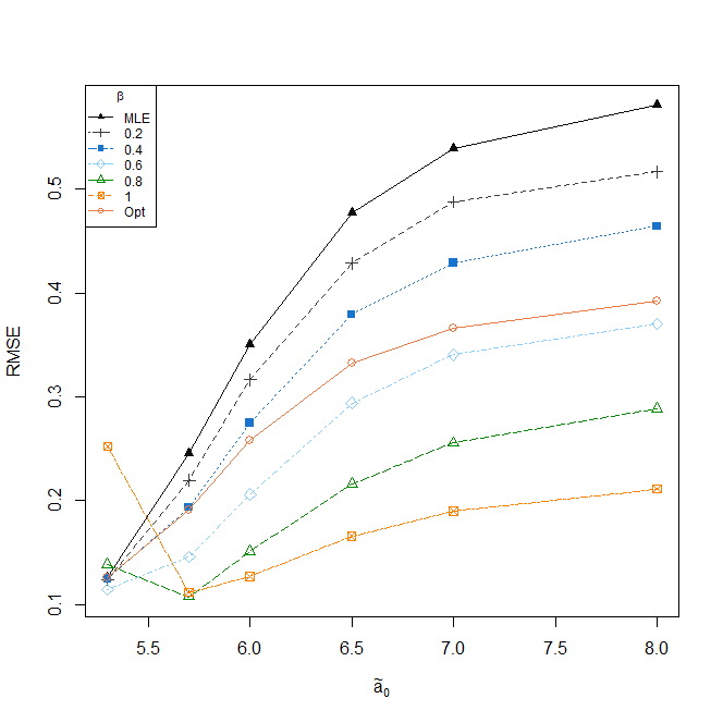
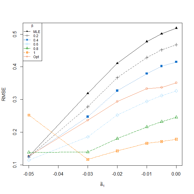
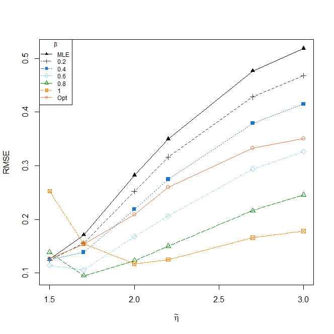
Figure 1: RMSE of the estimates under three types of contamination

We additionally compute the mean square error (MSE) of the estimates of reliability and mean lifetime of devices under a lower stress level $x_{0}=20.$ As expected, the estimated reliability and mean lifetime under contaminated scenarios are more accurate for positive values of $\alpha$.

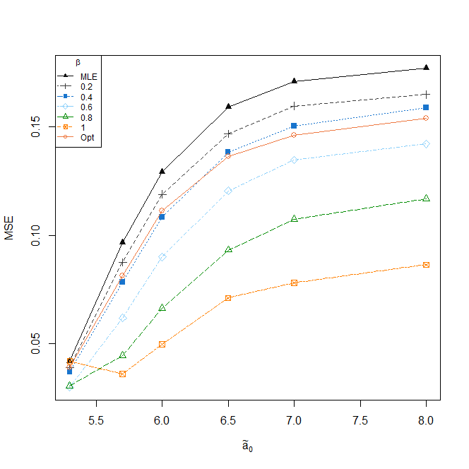
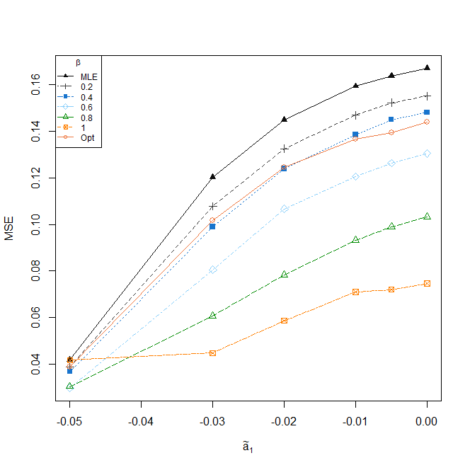
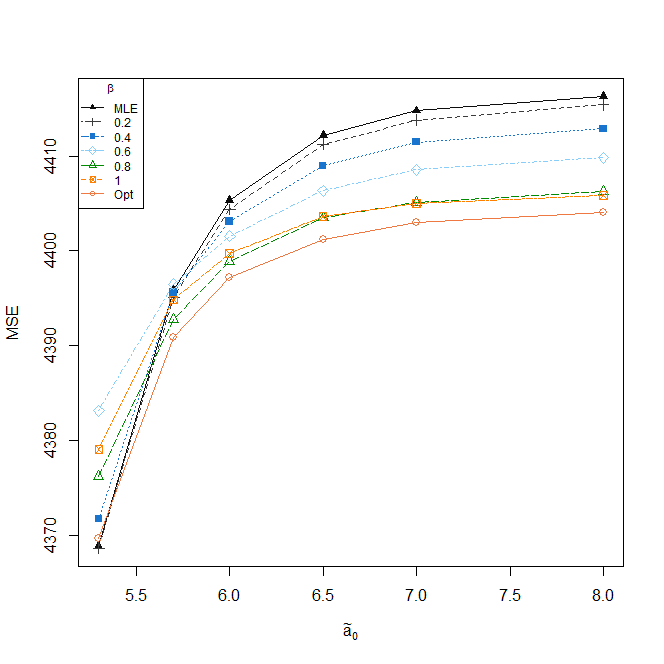
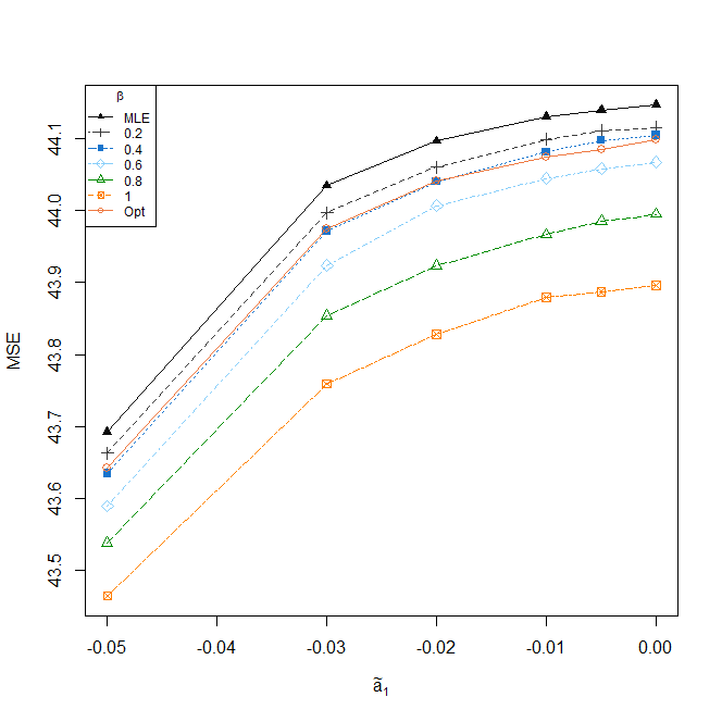
Figure 2: MSE of the reliability for $t=40$ (top) and mean lifetime ($\times 10^{2})$ (bottom) under normal operating conditions $x_{0}=20$ when the contamination is introduced on the first (left) and second (right) model parameters.

Further, we compare the direct and transformed asymptotic CIs of reliability and mean lifetime under a constant stress level $x_{0}=20$ in terms of coverage probability of the resulting intervals, in the three different scenarios of contamination. CIs based on MDPDEs with large values of the tuning parameter are more robust than CIs based on the classical MLE. Further, the transformed CI has slightly higher coverage probability in all scenarios, but the difference is especially striking in highly contaminated scenarios.

Table 1: Coverage of the direct and transformed CIs for reliability under contamination in the first parameter, for different values of the tuning parameter.

$a_{0}$	5.3	5.7	6	6.5	7	8
Direct CI
MLE	0.756	0.462	0.288	0.164	0.124	0.108
$\beta=$ 0.2	0.776	0.520	0.338	0.234	0.180	0.156
$\beta=$ 0.4	0.796	0.564	0.384	0.254	0.204	0.162
$\beta=$ 0.6	0.820	0.656	0.498	0.326	0.246	0.220
$\beta=$ 0.8	0.778	0.750	0.634	0.478	0.382	0.344
$\beta=$ 1	0.686	0.784	0.726	0.596	0.568	0.518
Optimal	0.772	0.536	0.370	0.232	0.204	0.158
Transformed CI
MLE	0.908	0.740	0.556	0.376	0.272
$\beta=$ 0.2	0.900	0.758	0.598	0.424	0.348	0.296
$\beta=$ 0.4	0.892	0.796	0.652	0.488	0.398	0.346
$\beta=$ 0.6	0.896	0.862	0.750	0.588	0.504	0.434
$\beta=$ 0.8	0.854	0.910	0.832	0.704	0.642	0.578
$\beta=$ 1	0.728	0.900	0.856	0.780	0.748	0.722
Optimal	0.896	0.780	0.640	0.468	0.384	0.332

Table 2: Coverage of the direct and transformed CIs for reliability under contamination in the second parameter, for different values of the tuning parameter.

$a_{1}$	-0.05	-0.03	-0.02	-0.01	-0.005	0
Direct CI
MLE	0.756	0.332	0.228	0.164	0.150	0.142
$\beta=$ 0.2	0.776	0.404	0.286	0.234	0.200	0.186
$\beta=$ 0.4	0.796	0.462	0.320	0.254	0.222	0.202
$\beta=$ 0.6	0.820	0.548	0.404	0.326	0.290	0.270
$\beta=$ 0.8	0.778	0.654	0.570	0.478	0.438	0.398
$\beta=$ 1	0.686	0.764	0.660	0.596	0.600	0.580
Optimal	0.772	0.410	0.290	0.232	0.224	0.202
Transformed CI
MLE	0.908	0.596	0.462	0.376	0.336	0.312
$\beta=$ 0.2	0.900	0.654	0.506	0.424	0.392	0.380
$\beta=$ 0.4	0.892	0.698	0.562	0.488	0.448	0.432
$\beta=$ 0.6	0.896	0.796	0.658	0.588	0.544	0.526
$\beta=$ 0.8	0.854	0.842	0.778	0.704	0.678	0.670
$\beta=$ 1	0.728	0.874	0.826	0.780	0.758	0.750
Optimal	0.896	0.686	0.552	0.468	0.436	0.418

Table 3: Coverage of the direct and transformed CIs for reliability under contamination in the third parameter, for different values of the tuning parameter.

$\eta$	1.5	1.7	2	2.2	2.7	3
Direct CI
MLE	0.756	0.620	0.400	0.290	0.164	0.144
$\beta=$ 0.2	0.776	0.690	0.458	0.344	0.234	0.186
$\beta=$ 0.4	0.796	0.714	0.518	0.388	0.256	0.202
$\beta=$ 0.6	0.820	0.780	0.590	0.498	0.326	0.270
$\beta=$ 0.8	0.778	0.824	0.718	0.634	0.478	0.398
$\beta=$ 1	0.686	0.782	0.770	0.728	0.596	0.582
Optimal	0.772	0.678	0.478	0.366	0.232	0.204
Transformed CI
MLE	0.908	0.856	0.678	0.556	0.376	0.312
$\beta=$ 0.2	0.900	0.862	0.700	0.598	0.426	0.380
$\beta=$ 0.4	0.892	0.888	0.752	0.652	0.492	0.432
$\beta=$ 0.6	0.896	0.916	0.818	0.750	0.588	0.526
$\beta=$ 0.8	0.854	0.906	0.874	0.828	0.704	0.670
$\beta=$ 1	0.728	0.858	0.884	0.860	0.780	0.750
Optimal	0.896	0.862	0.738	0.638	0.470	0.418

Table 4: Coverage of the direct and transformed CIs for mean lifetime under contamination in the first parameter, for different values of the tuning parameter.

$a_{0}$	5.3	5.7	6	6.5	7	8
Direct CI
MLE	0.756	0.462	0.288	0.164	0.124	0.108
$\beta=$ 0.2	0.776	0.520	0.338	0.234	0.180	0.156
$\beta=$ 0.4	0.796	0.564	0.384	0.254	0.204	0.162
$\beta=$ 0.6	0.820	0.656	0.498	0.326	0.246	0.220
$\beta=$ 0.8	0.778	0.750	0.634	0.478	0.382	0.344
$\beta=$ 1	0.686	0.784	0.726	0.596	0.568	0.518
Optimal	0.772	0.536	0.370	0.232	0.204	0.158
Transformed CI
MLE	0.932	0.726	0.546	0.366	0.276	0.234
$\beta=$ 0.2	0.938	0.754	0.598	0.416	0.348	0.304
$\beta=$ 0.4	0.952	0.792	0.642	0.496	0.412	0.354
$\beta=$ 0.6	0.970	0.868	0.760	0.584	0.510	0.476
$\beta=$ 0.8	0.954	0.926	0.832	0.716	0.656	0.596
$\beta=$ 1	0.880	0.944	0.888	0.794	0.756	0.730
Optimal	0.948	0.770	0.616	0.454	0.390	0.332

Table 5: Coverage of the direct and transformed CIs for mean lifetime under contamination in the second parameter, for different values of the tuning parameter.

$a_{1}$	-0.05	-0.03	-0.02	-0.01	-0.005	0
Direct CI
MLE	0.756	0.332	0.228	0.164	0.150	0.142
$\beta=$ 0.2	0.776	0.404	0.286	0.234	0.200	0.186
$\beta=$ 0.4	0.796	0.462	0.320	0.254	0.222	0.202
$\beta=$ 0.6	0.820	0.548	0.404	0.326	0.290	0.270
$\beta=$ 0.8	0.778	0.654	0.570	0.478	0.438	0.398
$\beta=$ 1	0.686	0.764	0.660	0.596	0.600	0.580
Optimal	0.772	0.410	0.290	0.232	0.224	0.202
Transformed CI
MLE	0.932	0.574	0.452	0.366	0.340	0.318
$\beta=$ 0.2	0.938	0.642	0.516	0.416	0.388	0.374
$\beta=$ 0.4	0.952	0.702	0.572	0.496	0.454	0.440
$\beta=$ 0.6	0.970	0.790	0.654	0.584	0.554	0.530
$\beta=$ 0.8	0.954	0.856	0.790	0.716	0.684	0.682
$\beta=$ 1	0.880	0.896	0.856	0.794	0.788	0.782
Optimal	0.948	0.666	0.556	0.454	0.436	0.418

Table 6: Coverage of the direct and transformed CIs for mean lifetime under contamination in the third parameter, for different values of the tuning parameter.

$\eta$	1.5	1.7	2	2.2	2.7	3
Direct CI
MLE	0.756	0.620	0.400	0.290	0.164	0.144
$\beta=$ 0.2	0.776	0.690	0.458	0.344	0.234	0.186
$\beta=$ 0.4	0.796	0.714	0.518	0.388	0.256	0.202
$\beta=$ 0.6	0.820	0.780	0.590	0.498	0.326	0.270
$\beta=$ 0.8	0.778	0.824	0.718	0.634	0.478	0.398
$\beta=$ 1	0.686	0.782	0.770	0.728	0.596	0.582
Optimal	0.772	0.678	0.478	0.366	0.232	0.204
Transformed CI
MLE	0.932	0.840	0.660	0.544	0.368	0.318
$\beta=$ 0.2	0.938	0.860	0.706	0.598	0.418	0.374
$\beta=$ 0.4	0.952	0.898	0.754	0.642	0.498	0.440
$\beta=$ 0.6	0.970	0.944	0.820	0.762	0.584	0.530
$\beta=$ 0.8	0.954	0.966	0.892	0.830	0.716	0.682
$\beta=$ 1	0.880	0.940	0.924	0.892	0.794	0.782
Optimal	0.948	0.878	0.748	0.614	0.456	0.418

In addition, we test different scenarios of contamination. In the first scenario, we generate an outlying cell in the third interval by decreasing the value of the first parameter, $\theta_{0},$ and at the second we perform similarly, but decreasing the second parameter $\theta_{1}$. In both cases, the lifetime rate $\lambda(\widetilde{\boldsymbol{\theta}})$ gets decreased; the smaller is the contaminated parameter, greater is the contamination.

9.2 Wald-type tests

We empirically evaluate the performance of the Wald-type test statistics based on the MDPDEs for different values of the tuning parameter in terms of empirical level and power. We set the simple step-stress model presented in Section 9, with $N=200$ devices and $L=13$ inspection times. We consider the hypothesis testing problem

$$\operatorname{H}_{0}:a_{2}=-0.05\hskip 14.22636pt\text{vs}\hskip 14.22636pt\operatorname{H}_{1}:a_{2}\neq-0.05.$$ (25)

and we fix the true value of the model parameter as $\boldsymbol{\theta}_{0}=(5.3,-0.05,1.5)$ verifying the null hypothesis (when computing the empirical level) and $\boldsymbol{\theta}_{0}=(5.3,-0.06,1.5)$ when computing the empirical power. The Wald-type test statistic associated with the test in (25) based on the MDPDE, $\widehat{\boldsymbol{\theta}}^{\beta},$ is defined using (16) with $\boldsymbol{m}(\boldsymbol{\theta})=a_{2}-0.05$ and the critical region of the test is as given in (17).

Moreover, to examine the robustness of the test, we contaminate the third cell following the three contamination scenarios discussed in Section 9. Figure 3 shows the empirical level (left) and power (right) of the test against cell contamination, when introducing contamination in the first parameter, $a_{1},$ (left), the second parameter, $a_{2}$ (middle), are the third (right). The empirical level and power are computed as the proportion of rejected Wald-type test statistics over $R=500$ replications of the model under the null hypothesis for a significance level of $\alpha=0.05$.

All Wald-type tests, based on MDPDEs with different values of the tuning parameter, perform similarly in the absence of contamination. However, Wald-type test statistics based on MDPDEs with large values of the tuning parameter are clearly more robust than the classical MLE in terms of empirical level, showing strong robustness in all contaminated scenarios. Conversely, the overall performance of all Wald-type test statistics, based on different values of the tuning parameter, is quite similar in terms of power. When the contamination is introduced in the two parameters which are not under test, $a_{0}$ and $\eta,$ the power of the test is higher for low values of the tuning parameter $\beta$, including the MLE. However, when introducing contamination on the second parameter, $a_{1},$ Wald-type test statistics with large values of $\beta$ outperform the classical MLE in terms of robustness. So, Wald-type test statistics based on the MDPDE with moderately large value of the tuning parameter offer an appealing alternative for the classical Wald-type test statistic based on the MLE, with a clear gain in robustness in terms of level while remaining competitive in terms of power.

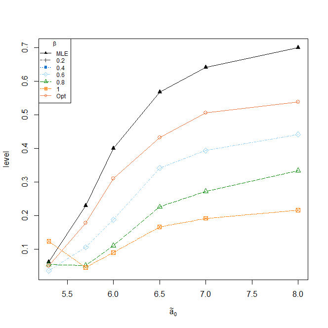
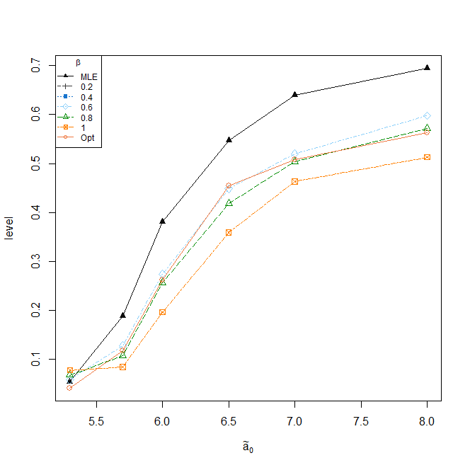
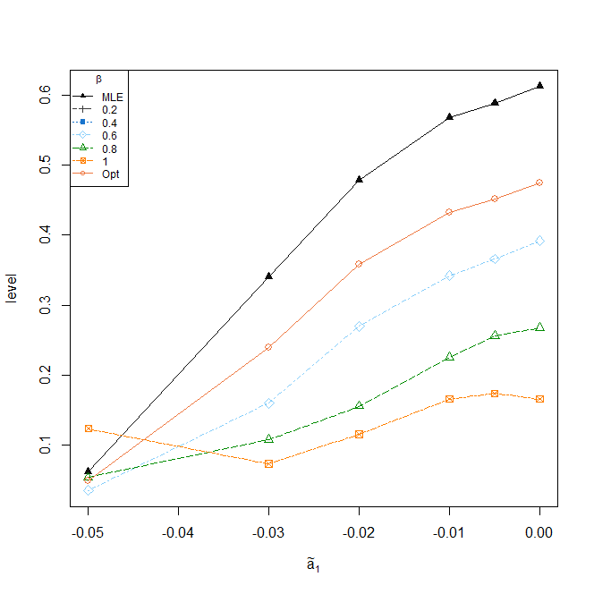
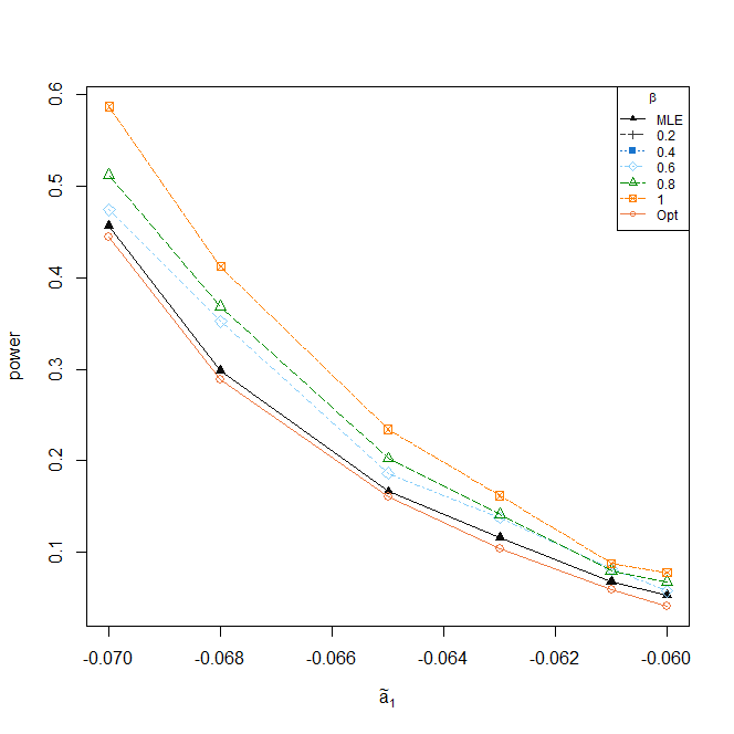
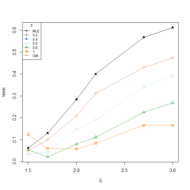
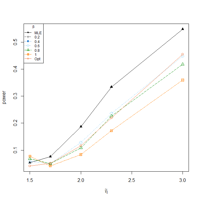
Figure 3: Empirical level(left) and power (right) of the Wald-type test

10 Real data analyses

We now illustrate the performance of the proposed robust methods in analyzing the influence of temperature in solar lighting devices (dataset 2.1) medium power silicon bipolar transistors (dataset 2.2) and LED lights (dataset 2.3).

10.1 Effect of temperature on solar lighting devices

We fit the step-stress ALT model with Weibull lifetime distributions for the first dataset 2.1 introduced in Section 2. Before fitting the model, the stress levels were normalized to $(0,1).$

Table 7 shows the estimated values of the model parameters with different values of the tuning parameter $\beta.$ Note that robust estimators tend to estimate slightly higher scale and shape parameters than the classical MLE. In addition, approximate CIs for the model parameters related to the scale, $a_{0}$ and $a_{1},$ are not too wide, indicating low variance of the estimators. The CI of the shape parameter $\eta$ includes the value of 1, and therefore we could not reject the null hypothesis of exponential lifetime distributions, at a confidence level of $95\%$. However, the estimated value of the shape parameter is away from 1 and so the Weibull lifetime would be more appropriate.

Table 7: Estimated values and approximate $95\%$ CIs for the model parameters with solar light data for different values of $\beta$

	$\widehat{a}_{0}^{\beta}$	IC($a_{0}^{\beta}$)	$\widehat{a}_{1}^{\beta}$	IC($a_{1}^{\beta}$)	$\widehat{\eta}^{\beta}$	IC($\eta^{\beta}$)
MLE	1.804	[1.697, 1.919]	-2.388	[-3.070, -1.707]	1.535	[0.882, 2.187]
$\beta=$ 0.2	1.812	[1.706, 1.924]	-2.380	[-3.060, -1.700]	1.497	[0.858, 2.137]
$\beta=$ 0.4	1.820	[1.712, 1.934]	-2.375	[-3.056, -1.695]	1.467	[0.836, 2.098]
$\beta=$ 0.6	1.826	[1.714, 1.946]	-2.372	[-3.055, -1.690]	1.441	[0.816, 2.066]
$\beta=$ 0.8	1.831	[1.711, 1.960]	-2.370	[-3.055, -1.685]	1.420	[0.799, 2.041]
$\beta=$ 1	1.836	[1.706, 1.976]	-2.370	[-3.057, -1.682]	1.401	[0.782, 2.020]

Table 8 presents the estimated mean lifetime, reliability at $t=400$ hours and $95\%$ distribution quantile for the solar light data with different values of the tuning parameter. Robust methods yield larger mean lifetimes (and consequently, smaller quantiles) than the classical MLE. However, all methods agree on the reliability of devices at 400 hours.

Table 8: Estimated mean lifetime (in hundred hours), reliability at $t=400$ hours and $95\%$ distributional quantile (in hundred hours) at a constant stress level $x_{0}=293K$ for solar light devices for different values of $\beta$

	$\operatorname{E}_{T}(\widehat{\boldsymbol{\theta}}^{\beta})$	$R_{4}(\widehat{\boldsymbol{\theta}}^{\beta})$	$Q_{0.95}(\widehat{\boldsymbol{\theta}}^{\beta})$
MLE	5.468	0.591	0.877
$\beta=$ 0.2	5.531	0.590	0.842
$\beta=$ 0.4	5.585	0.589	0.814
$\beta=$ 0.6	5.633	0.588	0.791
$\beta=$ 0.8	5.679	0.588	0.770
$\beta=$ 1	5.717	0.587	0.752

10.2 Effect of temperature on medium power silicon bipolar transistors

We now apply the proposed methods to the medium power silicon bipolar transistors dataset 2.2. To fit the multiple step-stress model, the temperature levels where normalized and the censored observations were removed.

Table 9 presents the estimated model parameters and the corresponding approximate CIs at $95\%$ confidence. In this case, the approximate CIs are very wide, implying high variance in the estimators. Robust estimators with large values of the tuning parameter of the first parameter $a_{0}$ are less than the classical one, and the behaviour is opposite when estimating $a_{1}$ and the shape $\eta.$ That difference is intensified when estimating the mean lifetime, reliability and $95\%$ quantile of devices, presented in Table 10. The estimated reliability of the transistors, mean lifetime and quantiles are clearly lower for robust methods. Applying Arrhenius model to the data, the estimated mean lifetime was over 90 years, a value reached by MDPDEs with large values of the tuning parameter.

Table 9: Estimated values and approximate $95\%$ CIs for the model parameters with medium power silicon transistors data for different values of $\beta$

	$\widehat{a}_{0}^{\beta}$	IC($a_{0}^{\beta}$)	$\widehat{a}_{1}^{\beta}$	IC($a_{1}^{\beta}$)	$\widehat{\eta}^{\beta}$	IC($\eta^{\beta}$)
MLE	16.434	[0.173, 1560.802]	-5.162	[-44.409, 34.085]	0.871	[0.000, 6.140]
$\beta=$ 0.2	14.981	[0.188, 1194.181]	-4.412	[-39.245, 30.421]	0.939	[0.000, 6.630]
$\beta=$ 0.4	14.880	[0.173, 1277.432]	-4.371	[-39.654, 30.913]	0.906	[0.000, 6.497]
$\beta=$ 0.6	14.823	[0.160, 1374.620]	-4.354	[-40.205, 31.497]	0.875	[0.000, 6.370]
$\beta=$ 0.8	14.068	[0.162, 1223.771]	-3.968	[-37.838, 29.903]	0.911	[0.000, 6.704]
$\beta=$ 1	13.452	[0.161, 1124.664]	-3.653	[-36.058, 28.753]	0.944	[0.000, 7.029]

Table 10: Estimated mean lifetime (in years), reliability at $t=80$ years and $95\%$ distribution quantile (in years) at a constant stress level $x_{0}=25\circ C$ for the medium power silicon transistors for different values of $\beta$

	$\operatorname{E}_{T}(\widehat{\boldsymbol{\theta}}^{\beta})$	$R_{80}(\widehat{\boldsymbol{\theta}}^{\beta})$	$Q_{0.95}(\widehat{\boldsymbol{\theta}}^{\beta})$
MLE	1678.749	0.928	51.657
$\beta=$ 0.2	376.774	0.787	15.507
$\beta=$ 0.4	346.944	0.759	12.463
$\beta=$ 0.6	334.164	0.738	10.469
$\beta=$ 0.8	153.596	0.563	5.648
$\beta=$ 1	81.490	0.365	3.410

10.3 Effect of temperature on Light Emitting Diodes (LEDs)

Finally, we report the performance of the proposed estimators in the dataset 2.3. The data are transformed to one-shot devices set-up and the stress levels are normalized as usual.

Table 11 presents the estimated coefficients for different values of the tuning parameter $\beta.$ Here, the shape parameter is moderately high, pointing out the appropriateness of using the Weibull lifetime distribution, instead of the exponential distribution. However, we must mention that approximate CIs are wide and that the value of 1 is included in the approximate CI for the shape parameter. Table 12 contains the estimated mean life, reliability at $t=2.88\times 10^{4}$ hours, and $95\%$ quantile based on the MDPDE for different values of $\beta$ under normal operating temperature. In this case, estimated mean lifetimes based on MDPDE with large values of $\beta$ are larger, implying higher reliability of the devices, and the same is true for the estimated reliability and quantiles. Note that the increment of such quantities gradually increases with $\beta,$ which is more in line with the results obtained in Zhao and Elsayed (2005).

Table 11: Estimated values and approximate $95\%$ CIs for the model parameters with LEDs data for different values of $\beta$.

	$\widehat{a}_{0}^{\beta}$	IC($a_{0}^{\beta}$)	$\widehat{a}_{1}^{\beta}$	IC($a_{1}^{\beta}$)	$\widehat{\eta}^{\beta}$	IC($\eta^{\beta}$)
MLE	10.093	[1.038, 98.179]	-4.894	[-33.559, 23.772]	1.882	[0.000, 8.794]
$\beta=$ 0.2	10.089	[1.026, 99.182]	-4.889	[-33.678, 23.901]	1.876	[0.000, 8.796]
$\beta=$ 0.4	10.092	[1.011, 100.770]	-4.890	[-33.875, 24.096]	1.883	[0.000, 8.853]
$\beta=$ 0.6	10.395	[0.907, 119.195]	-5.247	[-36.570, 26.076]	1.791	[0.000, 8.525]
$\beta=$ 0.8	10.166	[0.971, 106.458]	-4.970	[-34.671, 24.730]	1.897	[0.000, 8.953]
$\beta=$ 1	10.147	[0.972, 105.931]	-4.943	[-34.553, 24.667]	1.929	[0.000, 9.098]

Table 12: Estimated mean lifetime (in hours $\times 10^{4}$), reliability at $t=2.88\times 10^{4}$ hours and $95\%$ distributional quantile (in hours $\times 10^{4}$) at normal operating temperature $x_{0}=50\circ C$ for LEDs data with different values of $\beta$

	$\operatorname{E}_{T}(\widehat{\boldsymbol{\theta}}^{\beta})$	$R_{2.88}(\widehat{\boldsymbol{\theta}}^{\beta})$	$Q_{0.95}(\widehat{\boldsymbol{\theta}}^{\beta})$
MLE	2.146	0.249	0.499
$\beta=$ 0.2	2.138	0.247	0.495
$\beta=$ 0.4	2.143	0.248	0.499
$\beta=$ 0.6	2.908	0.451	0.623
$\beta=$ 0.8	2.308	0.297	0.544
$\beta=$ 1	2.264	0.283	0.547

11 Concluding remarks

In this paper, we have developed robust estimators and Wald-type test statistics for testing general composite null hypothesis based on the popular density power divergence (DPD) approach. We have examined the robustness properties of the proposed estimators and the test statistics theoretically as well as empirically, showing the clear improvement in terms of robustness with a small loss of efficiency in the absence of contamination. Further, point estimation and approximate CIs for the model parameters and some lifetime characteristics of interest based on the MDPDEs are derived, and their robustness in terms of accuracy (for the point estimation) and coverage probability (for the CIs) are empirically examined. Direct and transformed approximate CIs are also compared. Transformed CIs outperform the direct CIs, especially so in heavily contaminated scenarios. Finally, three real datasets from the reliability engineering field have been analyzed to illustrate the use of the proposed robust estimators and test statistics in practical situations.

Proof of the main results

Proof of the Result 1

Proof. As the MDPDE is a minimizer, it must satisfy the equation

$$\frac{\partial d_{\beta}\left(\widehat{\boldsymbol{p}},\boldsymbol{\pi}\left(\boldsymbol{\theta}\right)\right)}{\partial\boldsymbol{\theta}}=(\beta+1)\sum_{j=1}^{L+1}\left(\pi_{j}(\boldsymbol{\theta})^{\beta-1}\left(\pi_{j}(\boldsymbol{\theta})-\widehat{p}_{j}\right)\frac{\partial\pi_{j}(\boldsymbol{\theta})}{\partial\boldsymbol{\theta}}\right)=\boldsymbol{0}_{2}.$$

where

$$\frac{\partial\pi_{j}(\boldsymbol{\theta})}{\partial\boldsymbol{\theta}}=\frac{\partial G_{T}(t_{j})}{\partial\boldsymbol{\theta}}-\frac{G_{T}(t_{j-1})}{\partial\boldsymbol{\theta}}.$$

Now, setting as $x_{i}$ the stress level at which the units are tested before the $\tau_{i}-$th inspection time, with $\tau_{i-1}<t_{j}\leq\tau_{i},$ we have

$$\boldsymbol{z}_{j}=\frac{\partial G_{T}(t_{j})}{\partial\boldsymbol{\theta}} =g_{T}(t_{j})\begin{pmatrix}-(t_{j}+h_{i-1})\\ -(t_{j}+h_{i-1})x_{i}+h_{i-1}^{\ast}\\ \log\left(\frac{t_{j}+h_{i-1}}{\alpha_{i}}\right)\frac{t_{j}+h_{i-1}}{\eta}\end{pmatrix}$$

with $h_{i-1}^{\ast}$ as in (9). Defining the matrix $\boldsymbol{W}$ with rows $\boldsymbol{w}_{j}=\boldsymbol{z}_{j}-\boldsymbol{z}_{j-1},$ we obtain the desired result.

 

Proof of the Result 7

Proof. Let $\boldsymbol{\theta}_{0}$ be the true value of the model parameter satisfying the null hypothesis in (15). From Theorem 2, we know that

$$\sqrt{N}\left(\widehat{\boldsymbol{\theta}}^{\beta}-\boldsymbol{\theta}_{0}\right)\rightarrow\mathcal{N}\left(\boldsymbol{0},\boldsymbol{J}_{\beta}^{-1}(\boldsymbol{\theta}_{0})\boldsymbol{K}_{\beta}(\boldsymbol{\theta}_{0})\boldsymbol{J}_{\beta}^{-1}(\boldsymbol{\theta}_{0})\right)$$

from which it follows that

$$\sqrt{N}\boldsymbol{m}(\widehat{\boldsymbol{\theta}}^{\beta})\rightarrow\mathcal{N}\left(\boldsymbol{0},\boldsymbol{M}^{T}(\boldsymbol{\theta}_{0})\boldsymbol{J}_{\beta}^{-1}(\boldsymbol{\theta}_{0})\boldsymbol{K}_{\beta}(\boldsymbol{\theta}_{0})\boldsymbol{J}_{\beta}^{-1}(\boldsymbol{\theta}_{0})\boldsymbol{M}^{T}(\boldsymbol{\theta}_{0})\right).$$

Now, the covariance matrix $\boldsymbol{M}^{T}(\boldsymbol{\theta}_{0})\boldsymbol{J}_{\beta}^{-1}(\boldsymbol{\theta}_{0})\boldsymbol{K}_{\beta}(\boldsymbol{\theta}_{0})\boldsymbol{J}_{\beta}^{-1}(\boldsymbol{\theta}_{0})\boldsymbol{M}^{T}(\boldsymbol{\theta}_{0})$ has maximum rank, and then by transforming the variable $\sqrt{N}\boldsymbol{m}(\widehat{\boldsymbol{\theta}}^{\beta}),$ we obtain

$$N\boldsymbol{m}^{T}(\widehat{\boldsymbol{\theta}}^{\beta})\left(\boldsymbol{M}^{T}(\boldsymbol{\theta}_{0})\boldsymbol{J}_{\beta}^{-1}(\boldsymbol{\theta}_{0})\boldsymbol{K}_{\beta}(\boldsymbol{\theta}_{0})\boldsymbol{J}_{\beta}^{-1}(\boldsymbol{\theta}_{0})\boldsymbol{M}(\boldsymbol{\theta}_{0})\right)^{-1}\boldsymbol{m}(\widehat{\boldsymbol{\theta}}^{\beta})\rightarrow\chi^{2}_{r}.$$

As $\widehat{\boldsymbol{\theta}}^{\beta}$ is a consistent estimator of $\boldsymbol{\theta}_{0},$ the stated result follows.                                                                                                              

Proof of the Result 8

Proof. A first-order Taylor expansion of $\ell(\boldsymbol{\theta})=\ell^{\ast}(\boldsymbol{\theta},\boldsymbol{\theta}^{\ast})$ at $\widehat{\boldsymbol{\theta}}^{\beta}$ around $\boldsymbol{\theta}^{\ast}$ gives

$$\ell(\widehat{\boldsymbol{\theta}}^{\beta})-\ell(\boldsymbol{\theta}^{\ast})=\frac{\partial\ell(\boldsymbol{\theta})}{\partial\boldsymbol{\theta}^{T}}\bigg{|}_{\boldsymbol{\theta}=\boldsymbol{\theta}^{\ast}}\left(\widehat{\boldsymbol{\theta}}^{\beta}-\boldsymbol{\theta}^{\ast}\right)+o_{p}\left(\parallel\widehat{\boldsymbol{\theta}}^{\beta}-\boldsymbol{\theta}^{\ast}\parallel\right)$$

and therefore, from Result 2, it follows that

$$\sqrt{N}\left(\ell(\widehat{\boldsymbol{\theta}}^{\beta})-\ell(\boldsymbol{\theta}^{\ast})\right)\rightarrow\mathcal{N}\left(0,\sigma_{W_{N}(\boldsymbol{\theta}^{\ast})}\right).$$

Further, as $\widehat{\boldsymbol{\theta}}^{\beta}$ is a consistent estimator of the true parameter $\boldsymbol{\theta}^{\ast}$, we have

$$\sqrt{N}\left(W_{N}(\widehat{\boldsymbol{\theta}}^{\beta})-\ell(\boldsymbol{\theta}^{\ast})\right)\rightarrow\mathcal{N}\left(0,\sigma_{W_{N}(\boldsymbol{\theta}^{\ast})}\right).$$

Now, the power function is the probability of rejection given the critical region (17), and so we have

$$\beta_{N}\left(\boldsymbol{\theta}^{\ast}\right) =\mathbb{P}\left(W_{N}(\widehat{\boldsymbol{\theta}}^{\beta})>\chi_{r,\alpha}^{2}|\boldsymbol{\theta}=\boldsymbol{\theta}^{\ast}\right)$$

$$=1-\Phi\left(\frac{\sqrt{N}}{\sigma_{W_{N}(\boldsymbol{\theta}^{\ast})}}\left(\frac{\chi^{2}_{r,\alpha}}{N}-\ell^{\ast}(\boldsymbol{\theta}^{\ast},\boldsymbol{\theta}^{\ast})\right)\right).$$

 

Proof of the Result 10

Proof. Let us denote $\boldsymbol{F}_{\boldsymbol{\theta},\varepsilon}=(1-\varepsilon)F_{\boldsymbol{\theta}_{0}}+\varepsilon\Delta_{\boldsymbol{n}}$ for the perturbed distribution function with mass function $\boldsymbol{\pi}_{\varepsilon}(\boldsymbol{\theta}),$ and $\boldsymbol{\theta}_{\varepsilon}=\boldsymbol{T}_{\beta}(\boldsymbol{F}_{\boldsymbol{\theta},\varepsilon}).$ The MDPDE satisfies the estimating equations

$$\sum_{j=1}^{L+1}\pi_{j}(\boldsymbol{\theta}_{\varepsilon})^{\beta-1}\left[(\pi_{j}(\boldsymbol{\theta}_{\varepsilon})-\boldsymbol{\pi}_{\varepsilon,j}(\boldsymbol{\theta}))\frac{\partial\pi_{j}(\boldsymbol{\theta}_{\varepsilon})}{\partial\boldsymbol{\theta}}\right]=\boldsymbol{0}.$$ (26)

Now, differentiating (26), we get

$$\sum_{j=1}^{L+1} (\beta-1)\pi_{j}(\boldsymbol{\theta}_{\varepsilon})^{\beta-2}\frac{\partial\pi_{j}(\boldsymbol{\theta}_{\varepsilon})}{\partial\boldsymbol{\theta}}\frac{\partial\boldsymbol{\theta}_{\varepsilon}}{\partial\varepsilon}\left[(\pi_{j}(\boldsymbol{\theta}_{\varepsilon})-\boldsymbol{\pi}_{\varepsilon,j}(\boldsymbol{\theta}))\frac{\partial\pi_{j}(\boldsymbol{\theta}_{\varepsilon})}{\partial\boldsymbol{\theta}}\right]$$

$$+\pi_{j}(\boldsymbol{\theta}_{\varepsilon})^{\beta-1}\left[\left(\frac{\partial\pi_{j}(\boldsymbol{\theta}_{\varepsilon})}{\partial\boldsymbol{\theta}}\frac{\partial\boldsymbol{\theta}_{\varepsilon}}{\partial\varepsilon}-\frac{\boldsymbol{\pi}_{\varepsilon,j}(\boldsymbol{\theta})}{\partial\varepsilon}\right)\frac{\partial\pi_{j}(\boldsymbol{\theta}_{\varepsilon})}{\partial\boldsymbol{\theta}}+\left(\pi_{j}(\boldsymbol{\theta}_{\varepsilon})-\boldsymbol{\pi}_{\varepsilon,j}(\boldsymbol{\theta})\right)\frac{\partial^{2}\pi_{j}(\boldsymbol{\theta}_{\varepsilon})}{\partial\boldsymbol{\theta}^{2}}\frac{\partial\boldsymbol{\theta}_{\varepsilon}}{\partial\varepsilon}\right]=\boldsymbol{0}.$$

Then, using the fact that $\boldsymbol{\pi}_{0}(\boldsymbol{\theta})=\boldsymbol{\pi}(\boldsymbol{\theta}_{0})$ and evaluating at $\varepsilon=0$, we obtain

$$\sum_{j=1}^{L+1}\pi_{j}(\boldsymbol{\theta}_{0})^{\beta-1}\left[\left(\frac{\partial\pi_{j}(\boldsymbol{\theta}_{0})}{\partial\boldsymbol{\theta}}\right)^{2}\text{IF}\left(\boldsymbol{n},\boldsymbol{T}_{\beta},\boldsymbol{F}_{\boldsymbol{\theta}}\right)-\left(\frac{\partial\pi_{j}(\boldsymbol{\theta}_{0})}{\partial\boldsymbol{\theta}}\right)(-\pi_{j}(\boldsymbol{\theta}_{0})+\Delta_{\boldsymbol{n}})\right]=\boldsymbol{0}.$$

Now, rewriting this equation in matrix form, we get

$$\boldsymbol{W}^{T}D_{\boldsymbol{\pi}(\boldsymbol{\theta_{0}})}^{\beta-1}\boldsymbol{W}\cdot\text{IF}\left(\boldsymbol{n},\boldsymbol{T}_{\beta},\boldsymbol{F}_{\boldsymbol{\theta}}\right)-\boldsymbol{W}^{T}\boldsymbol{D}_{\boldsymbol{\pi}(\boldsymbol{\theta}_{0})}^{\beta-1}\left(-\boldsymbol{\pi}(\boldsymbol{\theta}_{0})+\Delta_{\boldsymbol{n}}\right)$$

and finally solving for $\text{IF}\left(\boldsymbol{n},\boldsymbol{T}_{\beta},\boldsymbol{F}_{\boldsymbol{\theta}}\right),$ we obtain the stated expression.

References

• [1] Balakrishnan, N. (2009). A synthesis of exact inferential results for exponential step-stress models and associated optimal accelerated life-tests. Metrika, 69(2), 351-396.
• [2] Balakrishnan, N., Castilla, E., Jaenada, M., & Pardo, L. (2022). Robust inference for non-destructive one-shot device testing under step-stress model with exponential lifetimes. arXiv preprint arXiv:2204.11560.
• [3] Balakrishnan, N., Castilla, E., Martin, N., $\&$ Pardo, L. (2019a). Robust estimators and test statistics for one-shot device testing under the exponential distribution. IEEE Transactions on Information Theory, 65(5), 3080–3096.
• [4] Balakrishnan, N., Castilla, E., Martin N. $\&$ Pardo, L. (2020a). Robust inference for one-shot device testing data under exponential lifetime model with multiple stresses. Quality and Reliability Engineering International, 36, 1916–1930.
• [5] Balakrishnan, N., Castilla, E., Martin, N., $\&$ Pardo, L. (2020b). Robust inference for one-shot device testing data under Weibull lifetime model. IEEE Transactions on Reliability, 69(3), 937–953.
• [6] Balakrishnan, N., Castilla, E. $\&$ Pardo, L. (2021). Robust statistical inference for one-shot devices based on density power divergences- An overview. In B. C. Arnold et al. (eds.), Methodology and Applications of Statistics, A Volume in Honor of C.R. Rao on the Occasion of his 100th Birthday. Springer, New York
• [7] Balakrishnan, N., & Ling, M. H. (2012). EM algorithm for one-shot device testing under the exponential distribution. Computational Statistics & Data Analysis, 56(3), 502-509.
• [8] Balakrishnan N. $\&$ Ling M.H. (2013). Expectation maximization algorithm for one shot device accelerated life testing with Weibull lifetimes, and variable parameters over stress. IEEE Transaction Reliability, 62(2), 537–551.
• [9] Balakrishnan, N., & Ling, M. H. (2012). Multiple-stress model for one-shot device testing data under exponential distribution. IEEE Transactions on Reliability, 61(3), 809-821.
• [10] Balakrishnan, N., & Ling, M. H. (2014). Best constant-stress accelerated life-test plans with multiple stress factors for one-shot device testing under a Weibull distribution. IEEE Transactions on Reliability, 63(4), 944-952.
• [11] Balakrishnan, N., Ling, M. H., $\&$ So, H. Y. (2021). Accelerated life testing of one-shot devices: Data Collection and Analysis. John Wiley $\&$ Sons, Hoboken, New Jersey.
• [12] Basak, S., Basu, A., & Jones, M. C. (2021). On the “optimal” density power divergence tuning parameter. Journal of Applied Statistics, 48(3), 536-556.
• [13] Basu, A., Harris, I. R., Hjort, N. L., & Jones, M. C. (1998). Robust and efficient estimation by minimising a density power divergence. Biometrika, 85(3), 549-559.
• [14] Basu, A., Mandal, A., Martin, N., & Pardo, L. (2016). Generalized Wald-type tests based on minimum density power divergence estimators. Statistics, 50(1), 1-26.
• [15] Bhattacharyya, G. K., & Soejoeti, Z. (1989). A tampered failure rate model for step-stress accelerated life test. Communications in Statistics-Theory and Methods, 18(5), 1627-1643.
• [16] Cai, B., Lin, X., & Wang, L. (2011). Bayesian proportional hazards model for current status data with monotone splines. Computational Statistics & Data Analysis, 55(9), 2644-2651.
• [17] DeGroot, M. H., & Goel, P. K. (1979). Bayesian estimation and optimal designs in partially accelerated life testing. Naval research logistics quarterly, 26(2), 223-235.
• [18] Fan, T. H., Balakrishnan, N., $\&$ Chang, C. C. (2009). The Bayesian approach for highly reliable electro-explosive devices using one-shot device testing. Journal of Statistical Computation and Simulation, 79(9), 1143-1154.
• [19] Gouno, E. (2001). An inference method for temperature step‐stress accelerated life testing. Quality and Reliability Engineering International, 17(1), 11-18.
• [20] Han, D., & Kundu, D. (2014). Inference for a step-stress model with competing risks for failure from the generalized exponential distribution under type-I censoring. IEEE Transactions on Reliability, 64(1), 31-43.
• [21] Hampel, F.R., Ronchetti, E., Rousseeuw, P.J., & Stahel, W. (1986). Robust Statistics: The Approach Based on Influence Functions John Wiley & Sons, New York.
• [22] Ling, M. (2019). Optimal design of simple step-stress accelerated life tests for one-shot devices under exponential distributions. Probability in the Engineering and Informational Sciences, 33(1), 121-135.
• [23] Ling, M. H. & Hu, X. W. (2020). Optimal design of simple step-stress accelerated life tests for one-shot devices under Weibull distributions. Reliability Engineering $\&$ System Safety, 193, 106630.
• [24] Meeter, C. A. & Meeker, W. Q. (1994). Optimum accelerated life tests with a nonconstant scale parameter. Technometrics, 36(1), 71–83.
• [25] Ling, M. H., So, H. Y., & Balakrishnan, N. (2015). Likelihood inference under proportional hazards model for one-shot device testing. IEEE Transactions on Reliability, 65(1), 446-458.
• [26] Meeker, W. Q., Escobar, L. A., $\&$ Lu, C. J. (1998). Accelerated degradation tests: modeling and analysis. Technometrics, 40(2), 89–99.
• [27] Nelson, W. (1980). Accelerated life testing-step-stress models and data analyses. IEEE Transactions on Reliability, 29(2), 103-108.
• [28] Warwick, J., $\&$ Jones, M. C. (2005). Choosing a robustness tuning parameter. Journal of Statistical Computation and Simulation, 75(7), 581-588.
• [29] Zhao, W., & Elsayed, E. A. (2005). A general accelerated life model for step-stress testing. IEEE Transactions, 37(11), 1059-1069.