Makespan Scheduling of Unit Jobs with Precedence Constraints in $O(1.995^{n})$ time

Abstract

In a classical scheduling problem, we are given a set of $n$ jobs of unit length along with precedence constraints and the goal is to find a schedule of these jobs on $m$ identical machines that minimizes the makespan. This problem is well-known to be NP-hard for an unbounded number of machines. Using standard 3-field notation, it is known as $P|\text{prec},p_{j}=1|C_{\max}$.

We present an algorithm for this problem that runs in $\mathcal{O}(1.995^{n})$ time. Before our work, even for $m=3$ machines the best known algorithms ran in $\mathcal{O}^{\star}(2^{n})$ time. In contrast, our algorithm works when the number of machines $m$ is unbounded. A crucial ingredient of our approach is an algorithm with a runtime that is only single-exponential in the vertex cover of the comparability graph of the precedence constraint graph. This heavily relies on insights from a classical result by Dolev and Warmuth (Journal of Algorithms 1984) for precedence graphs without long chains.

1 Introduction

Scheduling of precedence constrained jobs on identical machines is a central challenge in the algorithmic study of scheduling problems. In this problem, we have $n$ jobs, each one of unit length along with $m$ identical parallel machines on which we can process the jobs. Additionally, the input contains a set of precedence constraints of jobs; a precedence constraint $j^{\prime}\prec j$ states that job $j^{\prime}$ has to be completed before job $j$ can be started. The goal is to schedule the jobs non-preemptively so that the makespan is minimized. Here, the makespan is the time when the last job is completed. In the 3-field notation of Graham [19] this problem is denoted as $P\,|\,\mathrm{prec},p_{j}=1|\,C_{\max}$ .

Despite the extensive interest in the community [8, 13, 32] and plenty of practical applications [22, 24, 33] the exact complexity of the problem is still very far from being understood. Since the ’70s, it has been known that the problem is $\mathsf{NP}$-hard when the number of machines is the part of the input [34]. However, the computational complexity remains unknown even when $m=3$:

Open Problem 1 ([15]).

Is $P3|\text{prec},p_{j}=1|C_{\max}$ solvable in polynomial time?

In fact, this is one of the four unresolved open questions from the book by Garey and Johnson [15] and remains one of the most notorious open question in the area (see, e.g., [28, 26, 5]). While papers that solve different special cases of $P\,|\,\mathrm{prec},p_{j}=1|\,C_{\max}$ in polynomial time date back to 1961 [20], substantial progress on the problem was made very recently as well. In particular, a line of research initiated by Levey and Rothvoß [26, 27, 17], gives a quasi-polynomial approximation scheme for $Pm|\text{prec},p_{j}=1|C_{\max}$. In contrast to this, the exact (exponential time) complexity of the general problem has hardly been considered at all, to the best of our knowledge. We initiate such a study in this paper.

Natural dynamic programming over subsets of the jobs solves the problem in $\mathcal{O}^{\star}(2^{n}\binom{n}{m})$ time, and an obvious question is whether this can be improved. It is hypothesized that not all problems can be solved strictly faster than $\mathcal{O}^{\star}(2^{n})$ (where $n$ is some natural measure of the input size): the Strong Exponential Time Hypothesis (SETH) conjectures that $k$-SAT cannot be solved in $\mathcal{O}^{\star}(c^{n})$ time for any constant $c<2$. Breaking the $\mathcal{O}^{\star}(2^{n})$ barrier has been active research over the last years, with results including $\mathcal{O}^{\star}((2-\varepsilon)^{n})$ algorithms with $\varepsilon>0$ for Hamiltonian Cycle in undirected graphs [3], Bin Packing with a constant number of bins ([29]), and single machine scheduling with precedence constraints minimizing the total completion time [9]. We show that $P\,|\,\mathrm{prec},p_{j}=1|\,C_{\max}$ can be added to this list of problems:

Theorem 1.1.

$P\,|\,\mathrm{prec},p_{j}=1|\,C_{\max}$ admits an $\mathcal{O}(1.995^{n})$ time algorithm.

Note that Theorem 1.1 works even when the number of machines is given on the input. In that case, decreasing the base of the exponent is the best we can hope for with contemporary techniques. Namely, any $2^{o(n)}$ algorithm for $P\,|\,\mathrm{prec},p_{j}=1|\,C_{\max}$ would result in unexpected breakthrough for Densest $\kappa$-Subgraph-problem (see Appendix A) and a $2^{o(n)}$ time algorithm for the Biclique problem [21] on $n$-vertex graphs.

The starting point of our approach are two previous algorithms for $Pm|\text{prec},p_{j}=1|C_{\max}$. Recall that an (anti-)chain is a set of vertices that are pairwise (in-)comparable.

• Algorithm (A): An $\mathcal{O}(n^{h(m-1)+1})$ algorithm by Dolev and Warmuth [11], where $h$ is the maximum length of a chain (called the height).

• Algorithm (B): An $\mathcal{O}^{\star}(\#\mathrm{AC}\cdot\binom{n}{m})$ time folklore algorithm, where $\#\mathrm{AC}$ is the number of anti chains (see Theorem 5.7).

Algorithm (B) is a simple improvement of the aforementioned $\mathcal{O}^{\star}(2^{n}\binom{n}{m})$ time algorithm, where the dynamic programming table is indexed by only the elements of a subset that are maximal in the precedence order $\prec$. Algorithm (A) will be described in more detail below.

Intriguingly, Algorithm (A) and Algorithm (B) solve very different sets of instances quickly: A long chain cannot contribute much to the number of antichains since a chain and antichain can only overlap in one element. Optimistically, one may hope that a combination of (the ideas behind) these algorithms could make substantial progress on Open Problem 1 (by, for example, solving $P3|\text{prec},p_{j}=1|C_{\max}$ in $2^{o(n)}$).

In particular, a straightforward consequence of Dilworth’s theorem guarantees that $\#\mathrm{AC}$ is at most $\left(1+\frac{n}{a}\right)^{a}$, where $a$ is the cardinality of the largest antichain (see Claim 6). Focusing on the case when $m$ is a fixed constant, Algorithm (B) runs fast enough to achieve Theorem 1.1 whenever $a<0.97n$. This allows us to assume that the maximum antichain is of size at least $0.97n$ and therefore there are no chains of length more than $h=0.03n$. Unfortunately, even for constant $m$ this is still not good enough as Algorithm (A) would run in $n^{\Omega(n)}$ time.

However, the above argument gives us a stronger property: If we define $G^{\mathsf{comp}}$ as the comparability graph of the partial order, then in fact $G^{\mathsf{comp}}$ has a vertex cover of size at most $0.03n$. Our main technical contribution is that, when we parameterize $\prec$ by the size of the vertex cover of $G^{\mathsf{comp}}$ instead of by $h$, we can get a major improvement in the runtime. In particular, we get an algorithm with a single-exponential run time and polynomial dependence on $n$ and $m$:

Theorem 1.2.

$P\,|\,\mathrm{prec},p_{j}=1|\,C_{\max}$ admits $\mathcal{O}^{\star}(169^{|C|})$ time algorithm where $C$ is a vertex cover of the comparability graph of the precedence constraints.

Note that the fixed-parameter tractability in $|C|$ alone is not necessarily surprising or useful. To get that, one could for example guess the order in which the jobs from $C$ are processed and schedule the rest of the jobs in a greedy manner. This, unfortunately, would yield only a $|C|^{\mathcal{O}(|C|)}\cdot\mathrm{poly}(n)$ algorithm which is not enough to give any improvement over an exact $\mathcal{O}^{\star}(2^{n})$ algorithm in the general setting.

Since the runtime in Theorem 1.2 does not depend on the number of machines, Theorem 1.1 follows per the above discussion even when $m=\varepsilon n$ for some small constant $\varepsilon>0$: In such cases the binomial coefficient $\binom{n}{m}$ of Algorithm (B) is still small enough to yield an $\mathcal{O}(1.995^{n})$ time algorithm. For large $m>\varepsilon n$, we use a combination of the Subset Convolution technique and simple structural observations to design an $\mathcal{O}^{\star}(\#\mathrm{AC}+2^{n-m})$ time algorithm for $P\,|\,\mathrm{prec},p_{j}=1|\,C_{\max}$ . See also Figure 1.

Figure 1: Overview of use of algorithms for proving Theorem 1.1.

In the next paragraph, we sketch our insights behind the proof of Theorem 1.2.

Our approach for Theorem 1.2

The central inspiration of our algorithm is the following structural insight of the aforementioned $\mathcal{O}(n^{h(m-1)+1})$ time algorithm by Dolev and Warmuth [11]: let $z$ be the first time slot a sink (i.e., a job $v$ for which there is no precedence constraint $v\prec w$) is scheduled. Then, there exists an optimal schedule (which is called a zero-adjusted schedule) for which the set of jobs before and after timeslot $z$ can be reconstructed in polynomial time from the set of jobs scheduled at $z$. Equipped with this observation, Dolev and Warmuth [11] partition the schedule at timeslot $z$, (non-deterministically) guess the set of jobs scheduled at $z$ and construct two subproblems by deducing the set of jobs scheduled before and after $z$. Then, they show that each of these subproblems consists of a graph of height at least one less than the original graph and solve the subproblems recursively.

We extend the definition of zero-adjusted schedules and apply it to the setting of a small vertex cover. We let a sink moment be a moment in the schedule where at least one sink and at least one non-sink are scheduled. We define a sink-adjusted schedule where we require that after every sink moment only successors of the jobs in the sink moment and some sinks are processed. We also show that there always exists an optimal schedule that is sink-adjusted.

Key Insight: In a sink-adjusted schedule, for each non-sink $j$ processed at time $t$ there is a chain of predecessors of $j$ intersecting all the sink moments before $t$.

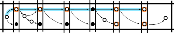
Figure 2: Illustration of Key Insight with an example of a sink-adjusted schedule. Sink-moments are distinguished between two bars. Jobs in the vertex cover are filled white (the remaining jobs are filled black). In a chain (highlighted blue) only one job is not in the vertex cover. If the set jobs of the vertex cover scheduled at sink moments (the orange jobs) are known, then the position of a job that is not a sink is roughly determined, due to the Key Insight.

Note that any chain can contain at most one vertex not from the vertex cover. Since we are allowed to make guesses about jobs in the vertex cover, we can guess which jobs of the vertex cover are in sink moments. Subsequently, for each non-sink job $j$ we can compute the maximum length of a chain of predecessors of $j$ that are processed in sink moments, and this maximum length indicates at or in between which sink moments $j$ is scheduled (up to a small error due to the unknown existence and location of one vertex not from the vertex cover in this chain).

We split the schedule at the moment $T^{\prime}$ where roughly half of the vertex cover jobs are processed. This creates two subproblems: one formed by all jobs scheduled before $T^{\prime}$ and one formed by all jobs scheduled after $T^{\prime}$. Then, we use that both of these subproblems admit a sink-adjusted schedule. For the vertex cover jobs we guess in which subproblem they are processed. We are left to partition the jobs that are not in $C$ and are sinks in the first subproblem or sources in the second subproblem (since for the remaining jobs, this is guessed or implied by the precedence constraints).

To determine this, we find a perfect matching on a bipartite graph. One side of this graph consists of the jobs for which it is still undetermined in which subproblem they are processed. On the other side we put the possible positions for these jobs in the subproblems. Edges of this graph indicate that a job can be processed at a given position. There are no precedence constraints between these unassigned jobs since all such jobs are not in the vertex cover, and therefore a perfect matching will correspond to a feasible schedule. How to find these positions and how to define the edges of this graph is not directly clear and will be explained in Section 4.

Related Work

The $P\,|\,\mathrm{prec},p_{j}=1|\,C_{\max}$ problem has been studied extensively from multiple angles throughout the last decades. Ullman [34] showed that it is $\mathsf{NP}$-complete via a reduction from $3$-SAT. Later, Lenstra and Rinnooy Kan [25] gave a somewhat simpler reduction from $k$-Clique.

The $P\,|\,\mathrm{prec},p_{j}=1|\,C_{\max}$ problem is known to be solvable in polynomial time for certain structured inputs. Hu [20] gave a polynomial time algorithm when precedence graph is a tree. This was later improved by Sethi [32] who showed that these instances can be solved in $\mathcal{O}(n)$ time. Garey et al. [16] considered a generalization when the precedence graph is an opposing forest, i.e., the disjoint union of an in-forest and out-forest. They showed that the problem is $\mathsf{NP}$-hard when $m$ is given as an input, and that the problem can be solved in polynomial time when $m$ is a fixed constant. Papadimitriou and Yannakakis [31] gave an $\mathcal{O}(n+m)$ time algorithm when the precedence graph is an interval order. Fujii et al. [12] presented the first polynomial time algorithm when $m=2$. Later, Coffman and Graham [8] gave an alternative $\mathcal{O}(n^{2})$ time algorithm for two machines. The runtime was later improved to near-linear by Gabow [13] and finally to truly linear by Gabow and Tarjan [14]. For a more detailed overview and other variants of $P\,|\,\mathrm{prec},p_{j}=1|\,C_{\max}$ , see the survey of Lawler et al [23].

Exponential Time / Parameterized Algorithms

A natural parameter for $P\,|\,\mathrm{prec},p_{j}=1|\,C_{\max}$ is the number of machines $m$. However, even showing that this parameterized problem is in $\mathsf{XP}$ would resolve Open Problem 1. Bodlaender and Fellows [5] show that problem is at least $\mathsf{W[2]}$-hard parameterized by $m$. Recently, Bodlaender et al. [6] showed that $P\,|\,\mathrm{prec},p_{j}=1|\,C_{\max}$ parameterized by $m$ is $\mathsf{XNLP}$-hard, which implies $\mathsf{W[t]}$-hardness for every $t$. Hence, a fixed-parameter tractable algorithm is unlikely.

Bessy and Giroudeau [2] showed that a problem called “Scheduling Couple Tasks” is FPT parameterized by the vertex cover of a certain associated graph. To the best of our knowledge, this is the only other result on the parameterized complexity of scheduling when the size of the vertex cover is considered to be a parameter.

Cygan et al. [9] study scheduling jobs of arbitrary length with precedence constraints on one machine and proposed an $\mathcal{O}((2-\varepsilon)^{n})$ time algorithm (for some constant $\varepsilon>0$). Similarly to our work, Cygan et al. [9] consider a dynamic programming algorithm over subsets and observe that a small maximum matching in the precedence graph can be exploited to significantly reduce the number of subsets that need to be considered.

Approximation

The $P\,|\,\mathrm{prec},p_{j}=1|\,C_{\max}$ problem was extensively studied through the lens of approximation algorithms, where the aim is to approximate the makespan. Recently, researchers analysed the problem in the important case when $m=\mathcal{O}(1)$. In a breakthrough paper, Levey and Rothvoß [26] developed a $(1+\varepsilon)$-approximation in $\exp\left(\exp\left(\mathcal{O}(\frac{m^{2}}{\varepsilon^{2}}\log^{2}\log n)\right)\right)$ time. This was subsequently improved by [17]. The currently fastest algorithm is due to Li [27] who improved the runtime to $n^{\mathcal{O}\left(\frac{m^{4}}{\varepsilon^{3}}\log^{3}\log(n)\right)}$. Interestingly, a key step in these approaches is that approximation is easy for instances of low height. A prominent open question is to give a PTAS even when the number of machines is fixed (see the recent survey of Bansal [1]).

Organization

In Section 2 we give short preliminaries. In Section 3 we extend the definition of zero-adjusted schedules from Dolev and Warmuth [11] to sink-adjusted schedules and discuss the structural insights of sink-adjusted schedules (with respect to a vertex cover). We prove Theorem 1.2 in Section 4 and subsequently we show how Theorem 1.2 implies Theorem 1.1 in Section 5. We provide concluding remarks in Section 6. Finally, we discuss (rather standard) lower bound for the problem in Appendix A.

2 Preliminaries

If $B$ is a Boolean, then $\llbracket B\rrbracket=1$ if $B$ is true and $\llbracket B\rrbracket=0$ if $B$ is false. We let $[N]$ denote the set of all integers $\{1,\dots,N\}$. We use $\widetilde{\mathcal{O}}(\cdot)$ notation to hide polylogarithmic factors and $\mathcal{O}^{\star}(\cdot)$ notation to hide polynomial factors in the input size.

Definitions related to the precedence constraints.

Let the input graph $G=(V,A)$ be a precedence graph. Importantly, throughout the paper we will assume that $G$ is its transitive closure, i.e. if $(u,v)\in A$ and $(v,w)\in A$ then $(u,w)\in A$. We will interchangeably use the notations for arcs in $G$ and the partial order, i.e. $(v,w)\in A\iff v\prec w$. Similarly, we use jobs to refer to the vertices of $G$.

The comparability graph $G^{\mathsf{comp}}=(V,E)$ of $G$ is the undirected graph obtained by replacing all directed arcs of $G$ with undirected edges. In other words, $v$ and $w$ are neighbors in $G^{\mathsf{comp}}$ if and only if they are comparable to each other. A set $X\subseteq V$ of jobs is a chain (antichain) if all jobs in $X$ are pairwise comparable (incomparable). For a job $v$, we denote $\textsf{pred}(v)\coloneqq\{u:u\prec v\}$ as the set of all predecessors of $v$ and $\textsf{pred}[v]\coloneqq\textsf{pred}(v)\cup v$. For a set of jobs $X$, we let $\textsf{pred}(X)\coloneqq\cup_{v\in X}\textsf{pred}(v)$ and $\textsf{pred}[X]\coloneqq\cup_{v\in X}\textsf{pred}[v]$. Similarly, we define $\textsf{succ}(v)\coloneqq\{u:v\prec u\}$, $\textsf{succ}[v]\coloneqq\textsf{succ}(v)\cup\{v\}$, $\textsf{succ}(X)\coloneqq\cup_{v\in X}\textsf{succ}(v)$ and $\textsf{succ}[X]\coloneqq\cup_{v\in X}\textsf{succ}[v]$.

The height $h(j)$ of a job $j$ is the length of the longest chain starting at job $j$, where length indicates the number of arcs in that chain. For example, the height of a job that has no successors is $0$. The height $h(G)$ of a precedence graph $G$ is equal to the maximum height of its jobs, i.e. $h(G)=\max_{j\in V}h(j)$. We call all jobs that have no successors sinks and all jobs that have to predecessors sources. For a set of jobs $X\subseteq V$ we denote $\textsf{sinks}(X)$ as all jobs of $X$ that have no successor within $X$ and $\textsf{sources}(X)$ as all jobs of $X$ that have no predecessor within $X$.

Schedules, dual graphs and dual schedules.

A schedule $\sigma=(S_{1},\dots,S_{T})$ for precedence graph $G=(V,A)$ on $m$ machines is a partition of $V$ such that $|S_{t}|\leq m$ for all $t\in[T]$ and for all $v\prec w$, if $v\in S_{t}$, $w\in S_{t^{\prime}}$, then $t<{t^{\prime}}$. We omit $G$ whenever it is clear from context. For a precedence graph $G=(V,A)$ we say that graph $\overleftarrow{G}=(V,\overleftarrow{A})$ is its dual if all the arcs of $G$ are directed in the opposite direction. We often explicitly use the fact that $\sigma=(S_{1},\dots,S_{T})$ is a schedule for $G$ if and only if the dual schedule $\overleftarrow{\sigma}=(S_{T},\dots,S_{1})$ is a schedule for $\overleftarrow{G}$.

Claim 1.

Let $\sigma=(S_{1},\dots,S_{T})$ be an optimal schedule for $G$. Then $\overleftarrow{\sigma}=(S_{T},\dots,S_{1})$ is an optimal schedule for $\overleftarrow{G}$.

Proof 2.1.

For any jobs $u,v\in V$ with $u\prec v$, we have that $v$ is processed after $u$ in $\sigma$. Hence, $v$ is processed before $u$ in $\overleftarrow{\sigma}$. Furthermore, any time slot in $\overleftarrow{\sigma}$ contains as most $m$ jobs. Hence, $\overleftarrow{\sigma}$ is a feasible schedule for $\overleftarrow{G}$. Schedule $\overleftarrow{\sigma}$ is also optimal: if not we could reverse $\overleftarrow{\sigma}$ and find a schedule with lower makespan for the original instance.

3 Sink-adjusted Schedules

We define a schedule $\sigma$ as a sequence of disjoint sets of jobs $S_{1},\dots,S_{T}$, such that a job in set $S_{i}$ is processed at time slot $i$; note that we do not need to know on which machine a job is scheduled since the machines are identical. Naturally, if $\sigma$ is feasible then $|S_{i}|\leq m$ for every $i\in[T]$. The makespan of such a schedule is $T$. For notation purposes, we use $S_{[a,b]}=\bigcup_{a\leq i\leq b}S_{i}$ to denote the set of jobs that are processed at a time-slot between $a$ and $b$.

Let us stress that we do not require that all input jobs to be in $S_{[1,T]}$. In fact, in the next sections, we will apply a divide-and-conquer technique and split the schedule into partial schedules. To be explicit about this, we use $V(\sigma)$ to denote the set $S_{[1,T]}$ of jobs assigned by $\sigma$. Naturally, a final feasible schedule needs to assign all the input jobs.

We prove that we can restrict our search to schedules with certain properties, by reusing and extending the definition of a zero-adjusted schedule from [11]. The definitions in the Section 3.1 will also be used to get an $\mathcal{O}^{\star}(2^{n-m}+\#\mathrm{AC})$ algorithm in Section 5. Next, in Section 3.2 we will consider properties of vertex cover of sink-adjusted schedules.

3.1 Definition and existence of sink-adjusted schedules

First, let us define the following sets for any schedule $\sigma=(S_{1}\dots,S_{T})$.

Definition 3.1 (Sets $Z_{t}$ and $H_{t}$).

For any time-slot $S_{t}$ of schedule $\sigma$, we define $Z_{t}\coloneqq S_{t}\cap\textsf{sinks}(V(\sigma))$ as all its jobs with zero height. We define set $H_{t}\coloneqq S_{t}\setminus\textsf{sinks}(V(\sigma))$ as all jobs in $S_{t}$ that have a height strictly greater than $0$.

We then define a sink-adjusted schedule as follows (see Figure 3):

Definition 3.2 (Sink-adjusted schedule and sink moments).

Let $\sigma=(S_{1},\ldots,S_{T})$. An integer $t\in[T]$ is a sink moment in the schedule $\sigma$ if $0<|H_{t}|<m$.

We say that schedule $\sigma$ is sink-adjusted if $(i)$ for every sink moment $t\in[T]$ all jobs in $S_{t+1},\ldots,S_{T}$ are either successors of some job in $S_{t}$, or are sinks (i.e., $S_{[t+1,T]}\subseteq\textsf{succ}(S_{t})\cup\textsf{sinks}(V(\sigma))$, and $(ii)$ all moments containing only sinks ($S_{i}\subseteq\textsf{sinks}(V(\sigma))$) are scheduled after every non-sink is scheduled.

Figure 3: Examples of three schedules with makespan $4$ and $m=2$. The sink-moments are highlighted in blue. Only the left schedule is sink-adjusted. The middle schedule is not sink-adjusted because the red jobs are sinks and are scheduled before a non-sink. The right schedule is not sink-adjusted because the red job is not a predecessor of any job in a trailing sink-moment.

Next, we prove that we can restrict our search for optimal schedules to sink-adjusted ones. The strategy behind the proof is to swap jobs until our schedule is sink-adjusted.

Theorem 3.3.

For every instance of $P\,|\,\mathrm{prec},p_{j}=1|\,C_{\max}$ , there exists an optimal schedule that is sink-adjusted.

Proof 3.4.

Take $\sigma=(S_{1},\dots,S_{T})$ to be an optimal schedule that is not sink-adjusted. First we prove property (ii). Let $t\in[T]$ be such that $S_{t}\subseteq\textsf{sinks}(V(\sigma))$, but there are non-sinks processed after $t$. Then take schedule $\sigma^{\prime}=(S_{1},\dots,S_{t-1},S_{t+1},\dots,S_{T},S_{t})$. In other words, we put the jobs from $S_{t}$ at the end of the schedule. Since $\sigma$ is optimal and the jobs in $S_{t}$ do not have any successors, $\sigma^{\prime}$ is also optimal. So take $\sigma=\sigma^{\prime}$. This step can be repeated until the second property holds.

Now we prove property (i). Let $\sigma$ be an optimal schedule that is not sink-adjusted and has the earliest $z\leq T$ such that $z$ is a sink moment, but $S_{[z+1,T]}\not\subseteq\textsf{succ}(S_{z})\cup\textsf{sinks}(V(\sigma))$. Note that all the jobs in $\textsf{succ}(S_{z})$ should be processed at or after $z+1$. Hence, there is a job $j$ with the following properties: (1) $j\in S_{i}$ for some $i\in[z+1,T]$, (2) $j$ is not a sink, (3) $j\not\in\textsf{succ}(S_{z})$ and (4) $\textsf{pred}(j)\cap S_{[z+1,T]}=\emptyset$. Property (4) holds because we can simply take the earliest job with properties (1-3).

Next, let us look at sink moment $z$. By definition it holds that $|H_{z}|<m$. This can happen because either $|Z_{z}|>0$ or $|S_{z}|<m$. In the first case $|Z_{z}|>0$, let $j^{\prime}$ be some job in $Z_{z}$. Observe that we can swap positions of $j$ and $j^{\prime}$ in the schedule. This new schedule is still feasible: $j^{\prime}$ can be processed later because it does not have any successors and $j$ can be processed earlier, because it does not have any predecessors at or after time $z$. Similarly, when $|S_{z}|<m$, job $j$ can be moved to empty slot in $S_{z}$. We can repeat this procedure until either $|S_{z}|=m$, $|S_{z}|=0$, or $S_{[z+1,T]}\subseteq\textsf{succ}(S_{z})\cup\textsf{sinks}(V(\sigma))$. Note that after this modification $\sigma$ remains an optimal schedule and none of the time slots before $z$ was changed. Because $z$ is not a sink moment anymore, the first sink moment is now after $z$. We can repeat this step until all sink moments satisfy the property (i).

The reader should think about these sink moments as guidelines in the sink-adjusted schedule that help us determine the positions of the jobs. Take for example the first sink moment $z$. If we know the $H_{z}$, then directly from Definition 3.2 we can deduce all the jobs that are processed before $z$ and all the jobs that are processed after $z$ (except some edge cases, see Section 4). Let us remark that the deduction of locations of jobs based on the $H_{z}$ was also used by Dolev and Warmuth [11].

3.2 The structure of sink-adjusted schedules versus the vertex cover

Now we assume that $C$ is a vertex cover of $G^{\mathsf{comp}}[V(\sigma)]$. We start with a simple observation about $C$:

Claim 2.

Any chain in $G[V(\sigma)]$ contains at most one vertex from $V(\sigma)\setminus C$.

Proof 3.5.

For the sake of contradiction, assume that there is a chain with two different jobs $v,w\in V\setminus C$. These jobs are comparable to each other, hence there exists an edge $\{v,w\}$ in the graph $G^{\mathsf{comp}}[V(\sigma)]$. However, this edge is not covered by $C$, which contradicts the fact that $C$ is a vertex cover of $G^{\mathsf{comp}}[V(\sigma)]$.

Recall that we assumed that $G$ is equal to its transitive closure. We define the depth of a vertex.

Definition 3.6 (Depth).

For a set $X\subseteq V$, the depth $0pt{X}{v}$ of a job $v\in V$ with respect to $X$ is the length of the longest chain in $G[X\cup\{v\}]$ that ends in $v$.

Recall, that we measure the length of a chain in its number of edges. Note that any source has depth $0$. For the remainder of this section, we assume that $\sigma=(S_{1},\dots,S_{T})$ is a sink-adjusted schedule. Next, we define the sinks moments of $\sigma$.

Definition 3.7 (Sink Moments of the Schedule).

Let $1\leq z(1)<\ldots<z(\ell)\leq T$ be the consecutive sink moments of $\sigma$. We let $\textsf{Imp}\coloneqq\bigcup_{i\in[\ell]}S_{z(i)}$ to be the set of all jobs in the sink moments of $\sigma$ (we set $z(0)\coloneqq 0$ and $z(\ell+1)\coloneqq T+1$ for convenience).

Define $\textsf{Low}\coloneqq C\cap\textsf{sinks}(V(\sigma))$ and let $\textsf{High}\coloneqq(C\cap\textsf{Imp})\setminus\textsf{Low}$. In other words, Low is the set of jobs from the vertex cover $C$ that are sinks and High is the set of jobs from $C$ that are processed during sink moments $z(1),\ldots,z(\ell)$, but are not sinks. Now, we show the following properties of jobs in High.

Property 3.8 (Jobs in High are almost determined).

If $v\in\textsf{High}$ is scheduled at timeslot $t$ (i.e., $v\in S_{t}$), then it must be that $t=z(0pt{\textsf{High}}{v}+1)$ or $t=z(0pt{\textsf{High}}{v}+2)$.

Proof 3.9.

Let us fix an arbitrary $v\in\textsf{High}$. By definition of High, we know that $v\in C$, $v\notin\textsf{sinks}(\sigma(V))$ and there exists $i\in[\ell]$ such that $v\in S_{z(i)}$. Because we assumed that the schedule $\sigma$ is sink-adjusted, for any sink moment $z(j)$ it holds that $S_{[z(j)+1,T]}\subseteq\textsf{succ}(S_{z(j)})\cup\textsf{sinks}(V(\sigma))$ where $j\in[\ell]$. This implies that $t=z(0pt{\textsf{Imp}}{v}+1)$. Note that $0pt{\textsf{Imp}}{v}\geq 0pt{\textsf{High}}{v}$ since $\textsf{High}\subseteq\textsf{Imp}$. Moreover, $0pt{\textsf{Imp}}{v}\leq 0pt{\textsf{High}}{v}+1$ since any chain in $G[\textsf{Imp}]$ can contain at most one vertex in $\textsf{Imp}\setminus\textsf{High}$ since such a vertex is either a sink or not in $C$, and in the last case Claim 2 applies.

Property 3.10 (Jobs in $C\setminus(\textsf{High}\cup\textsf{Low})$ are roughly determined).

Let $v\in C\setminus(\textsf{High}\cup\textsf{Low})$ be a vertex that is scheduled at moment $t\in[T]$ (i.e., $v\in S_{t}$), then $z(0pt{\textsf{High}}{v})<t<z(0pt{\textsf{High}}{v}+1)$ or $z(0pt{\textsf{High}}{v}+1)<t<z(0pt{\textsf{High}}{v}+2)$

Proof 3.11.

The proof is similar to that of Property 3.8. Let $v\in C\setminus(\textsf{High}\cup\textsf{Low})$. Hence, $v\in C$, $v\notin\textsf{sinks}(\sigma(V))$ and $v$ is not processed at any sink moment. Because we assumed that the schedule $\sigma$ is sink-adjusted, for any sink moment $z(j)$ it holds that $S_{[z(j)+1,T]}\subseteq\textsf{succ}(S_{z(j)})\cup\textsf{sinks}(V(\sigma))$ where $j\in[\ell]$. This implies that $z(0pt{\textsf{Imp}}{v})<t<z(0pt{\textsf{Imp}}{v}+1)$. Note that $0pt{\textsf{Imp}}{v}\geq 0pt{\textsf{High}}{v}$ since $\textsf{High}\subseteq\textsf{Imp}$. Moreover, $0pt{\textsf{Imp}}{v}\leq 0pt{\textsf{High}}{v}+1$ since any chain in $G[\textsf{Imp}]$ can contain at most one vertex in $\textsf{Imp}\setminus\textsf{High}$ since such a vertex is either a sink or not in $C$, and in the last case Claim 2 applies. Note that $v\in\textsf{High}\cup\textsf{Low}$, so $v$ cannot be processed at any sink moment. Hence the boundaries on $t$ follow.

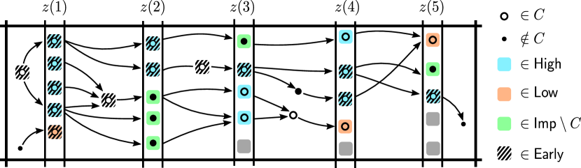
Figure 4: Figure presents a schedule with five sink moments $z(1),\ldots,z(5)$. Jobs from Vertex Cover are marked with a black ring (the remaining jobs are depicted with a black-filled circle). Set Imp contains every job in the sink-moment (highlighted either blue, green or red). Jobs from High are highlighted in blue. Jobs from Low are highlighted red. Jobs from $\textsf{Imp}\setminus C$ are highlighted green. Early jobs are wrapped with a solid black border. Gray rectangles are empty slots in the schedule. Observe that for a fixed chain there exists a single moment after which every job in it is late. This moment corresponds to the job from $\textsf{Imp}\setminus C$ on this chain.

Next, we define Early Jobs. See Figure 4 for example of High, Low and intuition behind Early jobs.

Definition 3.12 (Early Jobs).

We say a job $v\in S_{t}$ is early if either

$$v \in\textsf{High}\cup\textsf{Low} t =z(0pt{\textsf{High}}{v}+1),$$ and or

$$v \in C\setminus(\textsf{High}\cup\textsf{Low}) z(0pt{\textsf{High}}{v}))< t <z(0pt{\textsf{High}}{v}+1).$$ and

If a job is not early, we call it late. By Property 3.8, a late job $v$ in High is scheduled at $z(0pt{\textsf{High}}{v}+2)$. By Property 3.10 a late job $v$ in $C\setminus(\textsf{High}\cup\textsf{Low})$ is scheduled in between $z(0pt{\textsf{High}}{v}+1)$ and $z(0pt{\textsf{High}}{v}+2)$. Additionally it will be useful in Section 4 to know which jobs in Low are early and late in order to ensure that precedence constraints $v\prec w$ with $w\in\textsf{Low}$ and $v$ are not scheduled at the same sink moment.

Crucially, if we guess the set High of a sink-adjusted schedule $\sigma$, and which non-sink jobs are early and which non-sink jobs are late we can already deduce for each job in

$$\textsf{High}\cup(C\setminus(\textsf{High}\cup\textsf{Low}))\cup(V(\sigma)\setminus(C\cup\textsf{sinks}(V(\sigma)))=V(\sigma)\setminus\textsf{sinks}(V(\sigma))$$

on (or in between) which sink-moment it is scheduled.

Property 3.13 (Jobs in $V(\sigma)\setminus(C\cup\textsf{sinks}(V(\sigma)))$ are also roughly determined).

Let $v\in V(\sigma)\setminus(C\cup\textsf{sinks}(V(\sigma)))$ be a vertex that is scheduled at moment $t\in[T]$ (i.e., $v\in S_{t}$). Then $z(0pt{\textsf{High}}{v})<t\leq z(0pt{\textsf{High}}{v}+1)$.

Proof 3.14.

The proof is similar to that of Property 3.8. Let $v\in V(\sigma)\setminus(C\cup\textsf{sinks}(V(\sigma))$. Hence, $v\not\in C$, $v\notin\textsf{sinks}(V(\sigma))$. Note that $v$ might or might not be scheduled at a sink moment. Because we assumed that the schedule $\sigma$ is sink-adjusted, for any sink moment $z(j)$ it holds that $S_{[z(j)+1,T]}\subseteq\textsf{succ}(S_{z(j)})\cup\textsf{sinks}(V(\sigma))$ where $j\in[\ell]$. This implies that $z(0pt{\textsf{Imp}}{v})<t\leq z(0pt{\textsf{Imp}}{v}+1)$. Note that $0pt{\textsf{Imp}}{v}\geq 0pt{\textsf{High}}{v}$ since $\textsf{High}\subseteq\textsf{Imp}$. Moreover, $0pt{\textsf{Imp}}{v}\leq 0pt{\textsf{High}}{v}$ because $v\not\in C$ and thus $v$ is the only element in a chain ending in $v$ that is not in $C$ by Claim 2.

4 Single Exponential FPT Algorithm when Parameterized by Vertex Cover of the Comparability Graph

In this section we prove Theorem 1.2 and give an $\mathcal{O}^{\star}(169^{|C|})$ time algorithm for $P\,|\,\mathrm{prec},p_{j}=1|\,C_{\max}$ . We assume that the vertex cover $C\subseteq V$ of the comparability graph is given as input (if not, we can easily find it with the standard algorithm in $\mathcal{O}^{\star}(2^{|C|})$ time). Also, we assume that the deadline is $T$ and that there are exactly $m\cdot T$ jobs to be processed; this can be ensured by adding $m\cdot T-n$ jobs without any precedence constraints. Note that this operation does not increase the size of the vertex cover of $G^{\mathsf{comp}}$, as no edge is added to the precedence graph. Moreover, the number of added jobs is bounded by $n\cdot m\leq n^{2}$, which is only an additional polynomial factor in the running time. For convenience we use the following notation throughout this section:

Definition 4.1.

We call $(S_{1},\ldots,S_{T})$ a tight $m$-schedule for $G$ if the $S_{i}$’s partition $V(G)$ and for all $i\in[T]$ we have $|S_{i}|=m$.

If $G$ is clear from the context, it will be omitted. By the above discussion, we can restrict attention to detecting tight $m$-schedules.

4.1 Middle-adjusting schedules and their fingerprints

We will split the schedule at some time slot $T^{\prime}$ into two subproblems and solve them recursively. The issue with this approach is that even if we know which jobs are scheduled at time slot $T^{\prime}$ we still need to determine which jobs are scheduled before and after $T^{\prime}$. To assist us with this task, we restrict our search to schedules with a specific structure. We call these structure middle-adjusted schedule.

Definition 4.2 (Middle-adjusted Schedule).

We say that a schedule $\sigma=(S_{1},\ldots,S_{T})$ is middle-adjusted at timeslot $T^{\prime}$ if $\sigma_{L}\coloneqq(S_{1},\ldots,S_{T^{\prime}-1})$ and $\overleftarrow{\sigma_{R}}\coloneqq(S_{T},\ldots,S_{T^{\prime}+1})$ are both sink-adjusted.

Lemma 4.3.

For any tight $m$-schedule $\sigma=(S_{1},\ldots,S_{T})$ and time $T^{\prime}\in[T]$, there is a tight $m$-schedule $\sigma^{\prime}=(S^{\prime}_{1},\ldots,S^{\prime}_{T})$ middle-adjusted at timeslot $T^{\prime}$ such that $S^{\prime}_{T^{\prime}}=S^{\prime}_{T^{\prime}}$, $S^{\prime}_{[1,T^{\prime}-1]}=S_{[1,T^{\prime}-1]}$ and $S^{\prime}_{[T^{\prime}+1,T]}=S_{[T^{\prime}+1,T]}$.

Proof 4.4.

Let $\sigma_{L}:=(S_{1},\dots,S_{T^{\prime}-1})$ and $\overleftarrow{\sigma_{R}}:=(S_{T},\dots,S_{T^{\prime}+1})$. By Theorem 3.3, there are tight $m$-schedules of the instances $G[V(\sigma_{L})]$ and $G[V(\sigma_{R})]$ (with precedence constraints reversed) of $P\,|\,\mathrm{prec},p_{j}=1|\,C_{\max}$ that are sink-adjusted. Concatenating these schedules with $S_{T^{\prime}}$ in between results in a middle-adjusted schedule.

Our goal is to deduce the set of jobs processed at $\sigma_{L}$ and $\sigma_{R}$ based on the fact that our schedule is middle-adjusted and properties of the vertices of $C$ with respect to the schedule. Since $C$ is small, we can guess these properties with few guesses. The aforementioned properties are formalized in the following definition:

Definition 4.5 (Fingerprint).

Let $\sigma=(\sigma_{L},S_{T^{\prime}},\sigma_{R})$ be middle-adjusted schedule at $T^{\prime}$. Let

$$C_{L} \coloneqq V(\sigma_{L})\cap C,$$

$$C_{R} \coloneqq V(\sigma_{R})\cap C,$$

$$\textsf{Low}_{L} \coloneqq\textsf{sinks}(V(\sigma_{L}))\cap C_{L},$$

$$\textsf{Low}_{R} \coloneqq\textsf{sinks}(V(\overleftarrow{\sigma_{R}}))\cap C_{R},$$

$$\textsf{High}_{L} \coloneqq\{v\in C_{L}\setminus\textsf{sinks}(V(\sigma_{L})):v\textnormal{ scheduled at a sink moment of $\sigma_{L}$}\},$$

$$\textsf{High}_{R} \coloneqq\{v\in C_{R}\setminus\textsf{sinks}(V(\overleftarrow{\sigma_{R}})):v\textnormal{ scheduled at a sink moment of $\overleftarrow{\sigma_{R}}$}\},$$

$$\textsf{Early}_{L} \coloneqq\{v\in C_{L}:v\textnormal{ is early in $\sigma_{L}$}\},$$

$$\textsf{Early}_{R} \coloneqq\{v\in C_{R}:v\textnormal{ is early in $\overleftarrow{\sigma_{R}}$}\}.$$

We call $8$-tuple $(C_{L},C_{R},\textsf{Low}_{L},\textsf{Low}_{R},\textsf{High}_{L},\textsf{High}_{R},\textsf{Early}_{L},\textsf{Early}_{R})$ the fingerprint of $\sigma$.

The following will be useful to bound the runtime of our algorithm and is easy to check by case analysis:

Claim 3.

There are at most $13^{|C|}$ different fingerprints.

Proof 4.6.

Let $e\in C$. If $e\in C_{M}$ it cannot be in any of the other sets. If $e\in C_{L}$, it can be in $\textsf{High}_{L}$ and $\textsf{Low}_{L}$, but not in both. Additionally, independently it could be in $\textsf{Early}_{L}$. Thus, there are $3\cdot 2=6$ possibilities (see $C_{L}$ cell in Figure 5). Similarly, there are $6$ possibilities if $e\in C_{R}$. Thus in total there are $1+6+6=13$ possibilities per element in $C$.

Figure 5: Venn diagram of the sets often used in Section 4. Recall that by definition $I_{L}=\textsf{pred}(C_{L})\setminus C_{L}$ and $I_{R}=\textsf{succ}(C_{R})\setminus C_{R}$. The dashed area is equal to $U^{\prime}$, defined in Subsection 4.3.

4.2 The algorithm

An overview of the algorithm is described in Algorithm 1. It is given a precedence graph $G$, number of machines $m$, and a vertex cover $C$ of $G^{\mathsf{comp}}$ as input. The Algorithm outputs a tight $m$-schedule if it exists, and “False” otherwise.

Algorithm $\mathtt{schedule}(G,C,m)$

1 foreach $T^{\prime}\in[1,T]$ do

2       foreach fingerprint $f=(C_{L},C_{R},\textsf{Low}_{L},\textsf{Low}_{R},\textsf{High}_{L},\textsf{High}_{R},\textsf{Early}_{L},\textsf{Early}_{R})$ do

3             if $|C_{L}|,|C_{R}|\leq|C|/2$ then

4                   $(X_{L},X_{M},X_{R})\leftarrow\mathtt{divide}(G,m,T^{\prime},C,f)$

5                   $\sigma_{L}\leftarrow\mathtt{schedule}(G[C_{L}\cup X_{L}],C_{L},m)$

6                   $\sigma_{R}\leftarrow\mathtt{schedule}(G[C_{R}\cup X_{R}],C_{R},m)$

7                   if $\sigma=(\sigma_{L},C_{M}\cup X_{M},\sigma_{R})$ is a tight $m$-schedule for $G$ then

8                         return $\sigma$

return False

Algorithm 1 Algorithm for Theorem 1.2.

The first step of the algorithm is to guess integer $T^{\prime}\in[T]$ such that at most half of the jobs from $C$ are processed before $T^{\prime}$ and at most half of the jobs from $C$ are processed after $T^{\prime}$. Subsequently, we guess the fingerprint $f$ of a middle-adjusted schedule $(\sigma_{L},S_{T^{\prime}},\sigma_{R})$ Effectively, we guess for every job in $C$ whether it is processed in $\sigma_{L}$, at $T^{\prime}$ or in $\sigma_{R}$, and whether it is in Low, High and Early.

If we have guessed correctly, then we can deduce that jobs $\textsf{pred}(C_{L})\setminus C_{L}$ must be in $\sigma_{L}$ and the jobs in $\textsf{succ}(C_{R})\setminus C_{R}$ are in $\sigma_{R}$. We are not done yet, as the position of the remaining jobs from $V\setminus C$ is still not known. To solve this, we employ a subroutine $\mathtt{divide}$ that tells us for all jobs in $V\setminus C$ whether they are scheduled in $\sigma_{L}$, at $T^{\prime}$ or $\sigma_{R}$, by making use of the fingerprint. Formally:

Lemma 4.7.

There is a polynomial time algorithm $\mathtt{divide}$ that, given as input precedence graph $G$, integers $m,T^{\prime}\in\mathbb{N}$, vertex cover $C$ of $G^{\mathsf{comp}}$, and a fingerprint

$$f=(C_{L},C_{R},\textsf{Low}_{L},\textsf{Low}_{R},\textsf{High}_{L},\textsf{High}_{R},\textsf{Early}_{L},\textsf{Early}_{R}),$$

finds a partition $X_{L},X_{M},X_{R}$ of $V\setminus C$ with the following property: If $f$ is the fingerprint of a tight $m$-schedule $\sigma$ of $G$ that is middle-adjusted at time $T^{\prime}$, then $G[C_{L}\cup X_{L}]$ and $G[C_{R}\cup X_{R}]$ have tight $m$-schedules, $|X_{M}\cup(C\setminus(C_{L}\cup C_{R}))|=m$, $\textsf{pred}(C\setminus C_{R})\subseteq C_{L}\cup X_{L}$, and $\textsf{succ}(C\setminus C_{L})\subseteq C_{R}\cup X_{R}$.

This lemma will be proved in the next subsection.

With the partition of $V\setminus C$ into $X_{L},X_{M},X_{R}$ in hand, we can solve the associated two subproblems with substantially smaller vertex covers $C_{L}$ and $C_{R}$ recursively. If the combination results in a tight $m$-schedule we return it, and if such a schedule is never found we return “False” . This concludes the description of the algorithm, except the description of the subroutine $\mathtt{divide}$.

Run time analysis.

There are $13^{|C|}$ guesses for fingerprint $f$ in Algorithm 1. Additionally, there are at most $n$ possible guesses of $T^{\prime}$. After all guesses are successful, then in polynomial time we determine the set of jobs in $X_{L}$, $X_{M}$ and $X_{R}$ by Lemma 4.7 and with that, the jobs for the two subproblems: $C_{L}\cup X_{L}$ and $C_{R}\cup X_{R}$. Subsequently, we recurse, and solve these two instances of $P\,|\,\mathrm{prec},p_{j}=1|\,C_{\max}$ : one with jobs $C_{L}\cup X_{L}$ and one with $C_{R}\cup X_{R}$. Observe that by definition $C_{L}$ is a vertex cover of $C_{L}\cup X_{L}$ and $C_{R}$ is a vertex cover of $C_{R}\cup X_{R}$. Moreover $|C_{L}|,|C_{R}|\leq|C|/2$. Therefore, the total runtime $T(|C|)$ of the algorithm is bounded by:

$$T(|C|)\leq 13^{|C|}\cdot T\left(\frac{|C|}{2}\right)\cdot n^{\mathcal{O}(1)}.$$

Therefore, the total runtime of the algorithm is $T(|C|)\leq\mathcal{O}^{\star}(169^{|C|})$ as claimed.

Correctness.

We claim that $\mathtt{schedule}(G,C,m)$ returns a tight $m$-schedule if it exists, and that it returns “False” otherwise. Note that Algorithm 1 checks for feasibility in Line 1, so if there is no tight $m$-schedule it will always return “False”.

Thus, let us focus on the first part. Let $(S_{1},\ldots,S_{T})$ be a tight $m$-schedule. Let $T^{\prime}$ be the smallest integer such that $|S_{[1,T^{\prime}]}\cap C|\geq|C|/2$. Then by Lemma 4.3, there is a tight $m$-schedule $\sigma=(\sigma_{L},S_{T^{\prime}},\sigma_{R})$ that is middle adjusted at time $T^{\prime}$ such that $V(\sigma_{L})=S_{[1,T^{\prime}-1]}$. Consider the iteration of the loop at Line 1 where we pick the fingerprint of $\sigma$. By the choice $T^{\prime}$ we have that $|V(\sigma_{L})\cap C|,|V(\sigma_{R})\cap C|\leq|C|/2$, and hence the check at Line 1 is verified. Let $C_{M}=C\setminus(C_{L}\cup C_{R})$. By Lemma 4.7, we find $X_{L},X_{M},X_{R}$ such that $|X_{M}\cup C_{M}|=m$, there is a tight $m$-schedule $\sigma_{L}^{\prime}$ for $G[C_{L}\cup X_{L}]$ and a tight $m$-schedule $\sigma_{R}^{\prime}$ for $G[C_{R}\cup X_{R}]$. We claim that $\sigma^{\prime}=(\sigma_{L}^{\prime},(X_{M}\cup C_{M}),\sigma_{R}^{\prime})$ is a tight $m$-schedule and hence it will be output at Line 1. To see this, note we only need to check whether precedence constraints between vertices from different parts of the partition $V(\sigma_{L}^{\prime}),X_{M}\cup C_{M},V(\sigma_{R}^{\prime})$ are satisfied. Let $v\preceq w$ be such a constraint. Note that either $v\in C$ or $w\in C$ (or both), since $C$ is a vertex cover of $G^{\mathsf{comp}}$. If $v\in C$ then the constraint $v\prec w$ is satisfied since $v\in C_{L}$ or $\textsf{succ}(v)\subseteq V(\sigma_{R})$ by Lemma 4.7. Similarly, if $w\in C$ then the constraint $v\prec w$ is satisfied since $w\in C_{R}$ or $\textsf{pred}(v)\subseteq V(\sigma_{L})$. Thus $\sigma^{\prime}$ is a tight $m$-schedule and the correctness follows.

4.3 Dividing the jobs: The proof of Lemma 4.7

In this subsection we prove Lemma 4.7. Let us assume that $f$ is a fingerprint of a middle-adjusted schedule $\sigma\coloneqq(\sigma_{L},S_{T^{\prime}},\sigma_{R})$ at $T^{\prime}$ (hence $\sigma_{L}$ and $\overleftarrow{\sigma_{R}}$ are both sink-adjusted).

First of all, we can deduce that jobs in $I_{L}\coloneqq\textsf{pred}(C_{L})\setminus C_{L}$ must be processed in $\sigma_{L}$ because their successors are in $\sigma_{L}$. Similarly every job in $I_{R}\coloneqq\textsf{succ}(C_{R})\setminus C_{R}$ needs to be in $\sigma_{R}$. It remains to assign jobs in $U\coloneqq V\setminus(C\cup I_{R}\cup I_{L})$. For this, we will actually assign jobs from $U^{\prime}$ using a perfect matching on a bipartite graph, where

$$U^{\prime}\coloneqq U\cup(\textsf{Low}_{L}\setminus\textsf{Early}_{L})\cup(\textsf{Low}_{R}\setminus\textsf{Early}_{R}).$$

We show that for the jobs that are not in $U^{\prime}$, we know roughly where they are using the fingerprint and Properties 3.8, 3.10 and 3.13 for schedules $\sigma_{L}$ and $\overleftarrow{\sigma_{R}}$.

We will determine where the jobs from $U^{\prime}$ go using a perfect matching on a bipartite graph $H=((U^{\prime},P),F)$. The set $P\subset[T]\times[m]$ consists of positions at which the jobs of $U^{\prime}$ are processed in $\sigma$ and an edge $(u,(t,j))\in F$ will indicate that $u\in U^{\prime}$ can be processed at time $t\in[T]$. The ‘$j$’ indicates that it is the $j$th machine that will process the job.

We will claim later that we can independently determine for each job in $U^{\prime}$ whether it can be processed at a specific position in $P$. As such, finding a perfect matching of graph $H$ will determine the position of each job in $U^{\prime}$. Note that jobs in $U^{\prime}$ need not be assigned at their positions in $\sigma$ with this method, but they will be assigned at a position that will make an $m$-tight schedule.

Construction of $P$.

To construct this bipartite graph, we first find the set of possible positions $P$ where jobs from $U^{\prime}$ are processed. At $T^{\prime}$ the jobs from $C_{M}$ are processed, so there are $m-|C_{M}|$ jobs from $U^{\prime}$ processed there. We add positions $(T^{\prime},j)$ for $j\in[m-|C_{M}|]$ to $P$.

Let us now define the positions in $P$ for $t<T^{\prime}$, i.e. the positions in $\sigma_{L}$. Let $z_{L}$ be the first timeslot in $\sigma_{L}$ at which only sinks are processed. Since all jobs from $U^{\prime}$ are sinks in $\sigma_{L}$, they can only be processed at a sink moment of $\sigma_{L}$ or at or after $z_{L}$. Hence, to find the correct positions, we need the value of $z_{L}$ and the number of jobs from $U^{\prime}$ at each sink moment of $\sigma_{L}$. For this we first define blocks:

Definition 4.8.

Let $z(1),\dots,z(\ell)$ be the sink moments of $\sigma_{L}$. Then for $i\in[1,\ell]$ we define the $i$th block $B_{i}\coloneqq[z(i-1)+1,z(i)]$ and we let $B_{\ell+1}=[z(\ell)+1,T^{\prime}-1]$. Recall that $z(0)=0$. The length of a block $[l,r]$ is defined as $r-l+1$ (i.e., the length of the interval).

We will show that for many jobs, we can determine in which block they are processed.

Claim 4.

Let $\sigma$ be a middle-adjusted tight $m$-schedule. Given as input the precedence graph $G$, integer $m$, and fingerprint $f$ of $\sigma$ we can determine in polynomial time:

1. for $v\in\textsf{High}_{L}\cup(\textsf{Low}_{L}\cap\textsf{Early}_{L})$ at which time they are processed, and

2. for $v\in\textsf{pred}[C_{L}]\setminus(\textsf{Low}_{L}\setminus\textsf{Early}_{L})$ at which block they are processed,

3. the length of each block,

4. the value of $z_{L}$.

Proof 4.9.

For each job in $\textsf{High}_{L}$ we know whether it is early or late, so using Property 3.8 we know the exact sink moment it is processed, and as a consequence also in which block. For a job in $\textsf{Low}_{L}\cap\textsf{Early}_{L}$, we know by Definition 3.12 at which sink moment it is processed and as a consequence also in which block. Thus, to establish Item (1) we only need to determine when all sink moments are exactly (or in other words the length of each block).

For jobs in $C_{L}\setminus(\textsf{High}_{L}\cup\textsf{Low}_{L})$, we know whether it is early or late and we use Property 3.10 to find in which block it is processed. Recall that $I_{L}\coloneqq\textsf{pred}(C_{L})\setminus C_{L}$, so $I_{L}\subseteq V(\sigma_{L})\setminus(C_{L}\cup\textsf{sinks}(V(\sigma_{L}))$ as all jobs in $I_{L}$ are not in $C_{L}$ and they have some successor in $C_{L}$. Hence for any job in $I_{L}$, Property 3.13 tells us exactly in which block it is processed. This concludes the proof of Item (2).

Note that, by Item (2), all jobs from $V(\sigma_{L})$ for which we have not determined the block in which they are processed yet are all sinks in $\sigma_{L}$. Recall that $z_{L}$ is the first time slot such that $S_{z_{L}}\subseteq\textsf{sinks}(V(\sigma_{L}))$. Hence sinks from $\sigma_{L}$ can only be processed at sink moments of $\sigma_{L}$ or after or at $z_{L}$. Therefore, for each block $B_{i}$ with $i\leq\ell$ the only jobs that have not been assigned to it are at the sink moment $z(i)$. Hence, we can determine the length of each block as follows: If $n_{i}$ is the number of jobs from $\textsf{pred}[C_{L}]\setminus(\textsf{Low}_{L}\setminus\textsf{Early}_{L})$ in block $i$, then the length of block $i$ must be $\lceil n_{i}/m\rceil$. As a consequence, we do not only know at which sink moment the jobs from $\textsf{High}_{L}$ and $\textsf{Low}\cap\textsf{Early}$ are processed, but also at which time. This established Item (1) and Item (3).

Finally, for Item (4), we can compute the value $z_{L}$ by computing how many jobs from $\textsf{pred}[C_{L}]\setminus(\textsf{Low}_{L}\setminus\textsf{Early}_{L})$ are processed in the $(\ell+1)$th block; if the number of such jobs is $x$ then $z_{L}$ will be equal to $z(\ell)+\lceil x/m\rceil$, by the same reasoning as above.

We need to decide for each vertex in $U^{\prime}$ whether it is scheduled in $\sigma_{L}$, at $T^{\prime}$ or in $\sigma_{R}$. Note that the set $U^{\prime}\cap V(\sigma_{L})$ is equal to the set of jobs for which we do not know by Claim 4 at which block they are processed. As a consequence, if $u\in U^{\prime}$ is processed in $\sigma_{L}$, then it is a sink and it can only be processed at a sink moment or after or at $z_{L}$.

Let $z(i)$ be a sink moment of $\sigma_{L}$, we will describe how to compute $|S_{z(i)}\cap U^{\prime}|$, i.e. the number of positions that we need to create in the bipartite graph for time $z(i)$. Claim 4 gives the number of non-$U^{\prime}$ jobs within that block, say $n_{i}$. Hence, the number of positions at $z(i)$ for jobs from $U^{\prime}$ is equal to $(m-n_{i})\bmod m$. Therefore, we add $(z(i),j)$ to $P$ for all $j\in[(m-n_{i})\bmod m]$.

For all $t\in[z_{L},T^{\prime}-1]$ we create positions $(t,j)$ for every $j\in[m]$; each of these moments only contains sinks of $\sigma_{L}$. Note that all jobs processed at or after $z_{L}$ are jobs from $U^{\prime}$, as any job in $\textsf{Low}_{L}\cap\textsf{Early}_{L}$ is processed at some sink moment by definition of Early.

For the positions $t>T^{\prime}$ in $P$, we can use the same strategy. Note that by symmetry Claim 4 holds also for $\overleftarrow{\sigma_{R}}$. This way, we can find all possible positions for jobs of $U^{\prime}$ in a middle-adjusted schedule $\sigma$ in polynomial time, given $m$, the input graph and the fingerprint $f$ of $\sigma$.

Construction of edges $F$.

To define the edges of the bipartite graph $H$ and prove that any perfect matching on this bipartite graph relates to a feasible schedule, we will use the following claim.

Claim 5.

Given $T^{\prime}$, the fingerprint $f$ and precedence graph $G$, we can determine in polynomial time for each $v\in U^{\prime}$ an interval $[l_{v},r_{v}]$ such that

1. $\textsf{pred}(v)\setminus U^{\prime}$ is scheduled before $l_{v}$,

2. $\textsf{succ}(v)\setminus U^{\prime}$ is scheduled after $r_{v}$,

3. $v$ is scheduled in interval $[l_{v},r_{v}]$ in $\sigma$.

Furthermore if $u,v\in U^{\prime}$ and $u\prec v$ then $r_{u}<l_{v}$. Finally, if $u\in U^{\prime}$, $v\in C_{M}$ and $u\prec v$ then $r_{u}<T^{\prime}$ and similarly if $u\in U^{\prime}$, $v\in C_{M}$ and $v\prec u$ then $T^{\prime}<l_{u}$.

Proof 4.10.

Recall that $U^{\prime}$ is the union of $U$, $(\textsf{Low}_{L}\setminus\textsf{Early}_{L})$, and $(\textsf{Low}_{R}\setminus\textsf{Early}_{R})$. We will prove the claim for each of these three sets separately. The cases $v\in(\textsf{Low}_{L}\setminus\textsf{Early}_{L})$ and $v\in(\textsf{Low}_{R}\setminus\textsf{Early}_{R})$ are symmetric and we consider them first.

As before, let $\ell$ be the number of sink moments in $\sigma_{L}$ and $z(i)$ the time of the $i$th sink moment of $\sigma_{L}$. Let $k$ be the number of sink moments in $\overleftarrow{\sigma_{R}}$ and $y(i)$ the time of the $i$th sink moment of $\overleftarrow{\sigma_{R}}$ in $\sigma$. Let $z_{R}\in[T^{\prime}+1,T]$ be the first moment of $\sigma$ where a non-source of $V(\sigma_{R})$ is processed (see Figure 6 for schematic definition of positions $z(i),y(i)$ and $z_{L}$ and $z_{R}$). Define $z^{\prime}(i)$ as $z(i)$ for $i\in[\ell]$ and $z^{\prime}(\ell+1)=z_{L}$ and similarly $y^{\prime}(i)$ as $y(i)$ for $i\in[k]$ and $y^{\prime}(k+1)=z_{R}$.

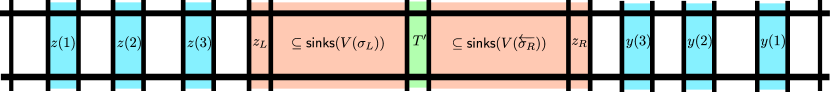
Figure 6: Definition of $z(i),y(i),z_{L}$ and $z_{R}$. Here $\ell$ and $k$ are equal $3$. Sink moments of $\sigma_{L}$ and $\overleftarrow{\sigma_{R}}$ are highlighted blue. Green is highlighted the moment $T^{\prime}$. In timeslots $[z_{L},T^{\prime}-1]$ and $[T^{\prime}+1,z_{R}]$ only sinks of $\sigma_{L}$ and $\overleftarrow{\sigma_{R}}$ are scheduled.

Case 1:

Let $v\in(\textsf{Low}_{L}\setminus\textsf{Early}_{L})$, in other words, $v\in C$, $v\in\textsf{sinks}(\sigma_{L})$ and $v$ is not early. For such a $v$ we take $l_{v}=z^{\prime}(0pt{\textsf{High}_{L}}{v}+2)$ and $r_{v}=T^{\prime}-1$. It is easy to see that all successors of $v$ are processed after $r_{v}$: $v$ is a sink in $\sigma_{L}$, so it has no successors in $\sigma_{L}$ and (2) follows.

Since $\sigma_{L}$ is sink-adjusted, we know that at any sink moment $t$ of $\sigma_{L}$ it holds that $S_{[t+1,T^{\prime}-1]}\subseteq\textsf{succ}(S_{t})\cup\textsf{sinks}(V(\sigma_{L}))$. Also, any chain can contain at most one vertex from $V\setminus C$ (Claim 2). Hence after $z^{\prime}(0pt{\textsf{High}_{L}}{v}+2)$ all predecessors of $v$ must be processed and (1) is indeed true.

By definition of earliness, $v$ is not processed at the $(0pt{\textsf{High}_{L}}{v}+1)$th sink moment of $\sigma_{L}$. Additionally, $v$ cannot be processed at a sink moment before $z^{\prime}(0pt{\textsf{High}_{L}}{v}+1)$, as at this sink moment its predecessors from $\textsf{High}_{L}$ are processed. Thus, since $v$ is processed in $\sigma_{L}$, (3) follows as well.

For $v\in(\textsf{Low}_{R}\setminus\textsf{Early}_{R})$ we define $l_{v}$ and $r_{v}$ in a similar way, using the properties of $\sigma_{R}$.

Case 2:

If $v\in U=V\setminus(C\cup I_{L}\cup I_{R})$, the definition of $l_{v}$ and $r_{v}$ is a bit less straightforward. We do this by defining four possible lower bounds. For notational simplicity, we let $\max\{\emptyset\}=0$.

$$l^{1}_{v} =\max\{z^{\prime}(i):\exists u\in(C_{L}\setminus(\textsf{High}_{L}\cup\textsf{Low}_{L}))\cap\textsf{pred}(v)\text{ in $i$th block of $\sigma_{L}$}\},$$

$$l^{2}_{v} =\max\{z(i)+1:\exists u\in\textsf{High}_{L}\cap\textsf{pred}(v)\text{ in $i$th sink moment of $\sigma_{L}$}\},$$

$$l^{3}_{v} =\begin{cases}T^{\prime}&\text{if }v\in\textsf{succ}(\textsf{Low}_{L}),\\ 0&\text{else,}\end{cases}\qquad l^{4}_{v}=\begin{cases}T^{\prime}+1&\text{if }v\in\textsf{succ}(C_{M}),\\ 0&\text{else.}\end{cases}$$

Similarly, for $r_{v}$ we define four upper bounds.

$$r^{1}_{v} =\min\{y^{\prime}(i):\exists u\in(C_{R}\setminus(\textsf{High}_{R}\cup\textsf{Low}_{R}))\cap\textsf{succ}(v)\text{ in $i$th block of $\overleftarrow{\sigma_{R}}$}\},$$

$$r^{2}_{v} =\min\{y(i)-1:\exists u\in\textsf{High}_{R}\cap\textsf{succ}(v)\text{ in $i$th sink moment of $\overleftarrow{\sigma_{R}}$ \}},$$

$$r^{3}_{v} =\begin{cases}T^{\prime}&\text{if }v\in\textsf{pred}(\textsf{Low}_{R}),\\ 0&\text{else,}\end{cases}\qquad r^{4}_{v}=\begin{cases}T^{\prime}-1&\text{if }v\in\textsf{pred}(C_{M}),\\ 0&\text{else.}\end{cases}$$

We then take $l_{v}=\max\{l^{1}_{v},l^{2}_{v},l^{3}_{v},l^{4}_{v}\}$ and $r_{v}=\min\{r^{1}_{v},r^{2}_{v},r^{3}_{v},r^{4}_{v}\}$. Note that the values of $l_{v}$ and $r_{v}$ can clearly be computed in polynomial time, as they are simple expressions that only depend on $f$ and $G$. See Figure 7 for schematic overview of lower and upper bounds.

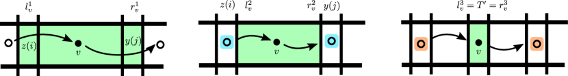
Figure 7: Schematic picture of determining lower bounds $l_{v}^{1},l_{v}^{2},l_{v}^{3}$ and $r_{v}^{1},r_{v}^{2},r_{v}^{3}$. We highlighted green the available intervals (e.g., $[l_{v}^{1},r_{v}^{1}]$) of job $v$. The first schema determines $l_{v}^{1}$ and $r_{v}^{1}$. For example, if vertex $u$ is in block $B_{i}$ then $l_{v}^{1}\geq z(i)$. Middle schema says that if $v$ has predecessor from High in sink-moment $z(i)$ then $l_{v}^{2}>z(i)$. Last condition simply says that if a sink in $V(\sigma_{L})$ is predecessor of $v$ then it needs to be processed at $T^{\prime}$ or later. Inequalities for $l_{v}^{4}$ and $r_{v}^{4}$ are similar to the last figure.

First we prove (1), the proof of (2) is similar. Let $u\in\textsf{pred}(v)\setminus U^{\prime}$, as a consequence $v\in\textsf{succ}(u)$. Because $v\not\in C$ we know $u\in C$. The vertex $u$ cannot be in $C_{R}$, as then we would have $v\in\textsf{succ}(C_{R})$, i.e. $v\in I_{R}$ and thus $v\not\in U^{\prime}$. If $u\in C_{M}$, then $u$ is processed at $T^{\prime}$ and before $l^{4}_{v}$. If $u\in C_{L}\setminus(\textsf{High}_{L}\cup\textsf{Low}_{L})$, $u$ cannot be processed at a sink moment of $\sigma_{L}$. If $u$ is processed at some $i$th block of $\sigma_{L}$ for $i<\ell$, it is therefore always processed before the $i$th sink moment because of bound $l_{v}^{1}$. If $u$ is processed at the $(\ell+1)$th block of $\sigma_{L}$, then it is definitely processed before $z^{\prime}(\ell+1)=z_{L}$ as it is not a sink in $\sigma_{L}$. Therefore, it is also processed before $l_{v}^{1}$. If $u\in\textsf{High}_{L}$, then $u$ is processed at a sink moment and before $l^{2}_{v}$. If $u\in\textsf{Low}_{L}$, then $u$ is processed in $\sigma_{L}$ and therefore before $l^{3}_{v}$.

For (3); we have to prove that $v$ is scheduled in interval $[l_{v},r_{v}]$ in $\sigma$. We show that $u$ is processed at or after $l_{v}$. To this end, it is sufficient to show that $u$ is processed after all lower bounds $l^{1}_{v}$, $l^{2}_{v}$, $l^{3}_{v}$ and $l^{4}_{v}$ separately. For $l^{1}_{v}$; if there is some $u\in(C_{L}\setminus(\textsf{High}_{L}\cup\textsf{Low}_{L}))\cap\textsf{pred}(v)$ at the $i$th block of $\sigma_{L}$, then it is processed somewhere strictly before $z^{\prime}(i)$ as it is not a sink of $\sigma_{L}$. Because $v$ must be processed at a sink moment or after $z_{L}$, it is processed at or after $z^{\prime}(i)$ in $\sigma$. For $l^{2}_{v}$; if there is some $u\in\textsf{High}_{L}\cap\textsf{pred}(v)$ at the $i$th sink moment, $v$ is processed after at some sink moment after $z(i)$ or after $z_{L}$. If $l^{3}_{v}=T^{\prime}$, then there is some $u\in\textsf{Low}_{L}$ such that $u\prec v$. Because $u$ is by definition a sink in $\sigma_{L}$, $v$ cannot be processed in $\sigma_{L}$. Therefore, $v$ is processed at or after $T^{\prime}$. If $l^{4}_{v}=T^{\prime}+1$, then there is some $u\in C_{M}$ such that $u\prec v$. Clearly, $v$ has to be processed at or after $T^{\prime}+1$. Hence $v$ is processed after of at $l_{v}$. The proof that $u$ is processed before or at $r_{v}$ is similar. This concludes the proof of Items (1-3).

It remains to show that condition $r_{u}<l_{v}$ holds if $u\prec v$ for every $u,v\in U^{\prime}$. Let $u,v\in U^{\prime}$ and $u\prec v$. At least one of $u$ or $v$ is in $C$. Recall that any job from $U^{\prime}$ in $\sigma_{L}$ is a sink in $\sigma_{L}$ and any job in $U^{\prime}$ is $\sigma_{R}$ is a sink in $\overleftarrow{\sigma_{R}}$. Therefore, when $u$ and $v$ are both in $C$, then $u\in\textsf{Low}_{L}$ and $v\in\textsf{Low}_{R}$ and by definition $l_{u}<r_{v}$. Now, let us assume that $u\in C$ and $v\not\in C$ (the proof is analogous when $u\notin C$ and $v\in C$). Then $u$ cannot be in $\textsf{Low}_{R}$ as $u\in\textsf{Low}_{R}$ and $u\prec v$ would imply $v\in I_{R}$ and thus $v\not\in U^{\prime}$. So, $u\in\textsf{Low}_{L}$ and $r_{u}=T^{\prime}-1$. Because $u\in\textsf{Low}_{L}$ and $u\in U^{\prime}$, by definition then $l_{v}\geq l^{3}_{v}=T^{\prime}>r_{u}$.

Note that if $u\in U^{\prime}$, $v\in C_{M}$ and $u\prec v$ then $r_{u}<T^{\prime}$ and similarly if $u\in U^{\prime}$, $v\in C_{M}$ and $v\prec u$ then $T^{\prime}<l_{u}$, because of the lower and upper bounds $l^{4}_{v}$ and $r^{4}_{v}$.

Given these $l_{v}$ and $r_{v}$ for each $v\in U^{\prime}$, we add an edge $(v,(t,j))$ to $F$ if and only if $(t,j)\in P$ and $l_{v}\leq t\leq r_{v}$.

The algorithm $\mathtt{divide}$.

We will now finish the proof of Lemma 4.7 by giving the algorithm $\mathtt{divide}$ in Algorithm 2 and proving that it has all properties of Lemma 4.7.

Algorithm $\mathtt{divide}(G,m,T^{\prime},C,f)$

1 $I_{L}\leftarrow\textsf{pred}(C_{L})\setminus C_{L}$, $I_{R}\leftarrow\textsf{succ}(C_{R})\setminus C_{R}$, $U\leftarrow(V\setminus(C\cup I_{L}\cup I_{R})$.

2 $U^{\prime}\leftarrow U\cup(\textsf{Low}_{L}\setminus\textsf{Early}_{L})\cup(\textsf{Low}_{R}\setminus\textsf{Early}_{R})$

3 Compute $P$ and $F$

4  // as discussed in Section 4.3

5 Construct bipartite graph $H=((P,U^{\prime}),F)$

6 $\mathcal{M}\leftarrow\mathtt{MaximumMatching}(H)$

7 if $\mathcal{M}$ is a perfect matching then

8       $X_{L}\coloneqq I_{L}\cup\{v\in U:\{v,(t,j)\}\in\mathcal{M},t\in[1,T^{\prime}-1]\}$

9       $X_{M}\coloneqq\{v\in U:\{v,(t,j)\}\in\mathcal{M},t=T^{\prime}\}$

10       $X_{R}\coloneqq I_{R}\cup\{v\in U:\{v,(t,j)\}\in\mathcal{M},t\in[T^{\prime}+1,T]\}$

11       return $(X_{L},X_{M},X_{R})$

return False

Algorithm 2 Algorithm for Lemma 4.7.

Clearly, $\mathtt{divide}$ runs in polynomial time as it construct graph $H$ using Claims 4 and 5 (which both take polynomial time) and then computes a perfect matching of $H$. We are left to show that if $f=(C_{L},C_{R},\textsf{Low}_{L},\textsf{Low}_{R},\textsf{High}_{L},\textsf{High}_{R},\textsf{Early}_{L},\textsf{Early}_{R})$ is the fingerprint of a tight $m$-schedule $\sigma$ of $G$ that is middle-adjusted at time $T^{\prime}$, then the partition $X_{L},X_{M},X_{R}$ of $V\setminus C$ returned by $\mathtt{divide}$ has the following properties: $G[C_{L}\cup X_{L}]$ and $G[C_{R}\cup X_{R}]$ have tight $m$-schedules, $|X_{M}\cup C_{M}|=m$, $\textsf{pred}(C\setminus C_{R})\subseteq C_{L}\cup X_{L}$, and $\textsf{succ}(C\setminus C_{L})\subseteq C_{R}\cup X_{R}$.

First, we prove that $\mathtt{divide}$ returns a partition at all. In other words, we show that the bipartite graph $H$ has a perfect matching. We claim there is a perfect matching of $H$ based on $\sigma$. By matching vertices to any position at the time slot they are processed in $\sigma$, we get a perfect matching. These edges must exist in $H$ because of (3) in Claim 5.

Because by construction there are $m-|C_{M}|$ position in $P$ with $t=T^{\prime}$ and $\mathcal{M}$ is a perfect matching, $|X_{M}\cup C_{M}|=m$.

Next, we prove $G[C_{L}\cup X_{L}]$ has a tight $m$-schedule. Take $\sigma_{L}$ and remove any jobs from $U^{\prime}$. This leaves exactly the positions in the set $P$ to be empty by Claim 4. Then construct the schedule $\sigma_{L}^{\prime}$ by processing each job $v\in U^{\prime}$ at the timeslot a job $v$ is matched to in the matching $\mathcal{M}$. More precisely, let $v\in U^{\prime}$ be matched to some position $(t,j)$ for $t<T^{\prime}$ by $\mathcal{M}$, then process $v$ at time $t$ in $\sigma_{L}^{\prime}$. Because of properties (1-2) of Claim 5, we know that all jobs in $\textsf{pred}(v)\setminus U^{\prime}$ are scheduled before $l_{v}\leq t$ and all jobs in $\textsf{succ}(v)\setminus U^{\prime}$ are processed after $r_{v}\geq t$. Furthermore, if there is some $u\in U^{\prime}$ that is comparable to $v$, then we know that their intervals imply the precedence constraints. Finally, since $\mathcal{M}$ is a perfect matching, all positions are filled. Hence, we have a tight $m$-schedule. With similar arguments $G[C_{R}\cup X_{R}]$ has a tight $m$-schedule.

It remains to show $\textsf{pred}(C\setminus C_{R})\subseteq C_{L}\cup X_{L}$. Take $v\in\textsf{pred}(C\setminus C_{R})=\textsf{pred}(C_{L}\cup C_{M})$. If $v\in\textsf{pred}(C_{L})$ then $v\in C_{L}\cup I_{L}\subseteq C_{L}\cup X_{L}$. If $v\in\textsf{pred}(C_{M})$, then by Claim 5 we have $r_{v}<T^{\prime}$ and so $v\in C_{L}\cup X_{L}$. Similarly we can show that $\textsf{succ}(C\setminus C_{L})\subseteq C_{R}\cup X_{R}$.

This concludes the proof of Lemma 4.7.

5 Getting below $2^{n}$: Proof of Theorem 1.1

In this section we give the present the two exact algorithms needed to prove our main result, Theorem 1.1. We first give an $\mathcal{O}^{\star}(2^{n})$ time algorithm using Fast Subset Convolution for $P\,|\,\mathrm{prec},p_{j}=1|\,C_{\max}$ in Subsection 5.1. We then improve this result and give an $\mathcal{O}^{\star}(\#\mathrm{AC}+2^{n-m})$ algorithm in Subsection 5.2. In Subsection 5.3 we present a natural Dynamic Programming algorithm that runs in $\mathcal{O}^{\star}(\#\mathrm{AC}\binom{n}{m})$. In Subsection 5.4 we prove that these algorithms together with Theorem 1.2 can be combined into an algorithm solving $P\,|\,\mathrm{prec},p_{j}=1|\,C_{\max}$ in $\mathcal{O}(1.995^{n})$ time.

5.1 An $\mathcal{O}^{\star}(2^{n})$ algorithm using Fast Subset Convolution

In this subsection, we show how to use Fast Subset Convolution to solve $P\,|\,\mathrm{prec},p_{j}=1|\,C_{\max}$ in $\mathcal{O}^{\star}(2^{n})$ time.

Theorem 5.1.

$P\,|\,\mathrm{prec},p_{j}=1|\,C_{\max}$ can be solved in time $\mathcal{O}^{\star}(2^{n})$.

This is a base-line of our methods. Later, we will then use this algorithm to get a faster than $\mathcal{O}^{\star}(2^{n})$ algorithm in the case $m\geq n/236$ in Subsection 5.2. To prove Theorem 5.1 let us first recall what we can do with fast subset convolutions.

Theorem 5.2 (Fast subset convolution with Zeta/ Möbius transform [4]).

Given functions $f,g:2^{U}\rightarrow\mathbb{N}$. There is an algorithm that computes

$$(f\circledast g)(S)\coloneqq\sum_{T\subseteq S}f(T)\cdot g(S\setminus T)$$

for every $S\subseteq U$ in $2^{|U|}\cdot|U|^{\mathcal{O}(1)}$ ring operations.

We will use this convolution multiple times in our algorithm. The plan is to encode the set of jobs $V$ as the universe $U$. Then the $f$ function will encode whether it is possible to process the jobs of $X\subseteq V$ within a given time frame. Function $g$ will be used to check whether the set of jobs $Y\subseteq V$can be processed at the last time-slot. We define these function formally.

For any $X\subseteq V$ and $t\in[T]$ let

$$f_{t}(X)\coloneqq\begin{cases}1&\text{if jobs $\textsf{pred}[X]$ can be processed within first $t$ time slots, and $X=\textsf{pred}[X]$},\\ 0&\text{otherwise.}\end{cases}$$

For any $Y\subseteq V$ define

$$g(Y)\coloneqq\begin{cases}1&\text{ if }|Y|\leq m\text{ and }Y\text{ is an antichain },\\ 0&\text{ otherwise,}\end{cases}$$

Note that the value $f_{T}(V)$ tells us whether the set of jobs can be processed within $T$ time units and is therefore the solution to our problem. Additionally, observe that the base-case $f_{0}(X)$ can be efficiently determined for all $X\subseteq V$ because $f_{0}(X)=1$ if $X=\emptyset$ and $f_{0}(X)=0$ otherwise. Moreover, for a fixed $Y\subseteq V$, the value of $g(Y)$ can be found in polynomial time.

It remains to compute $f_{t}(X)$ for every $t>0$. To achieve this, we define an auxiliary function $h_{t}:2^{V}\rightarrow{\rm Nature}$. For every $Z\subseteq V$, let

$$h_{t}(Z)\coloneqq\sum_{X\subseteq Z}f_{t-1}(X)\cdot g(Z\setminus X).$$

Once all values of $f_{t-1}(X)$ are known, the values of $h_{t}(Z)$ for $Z\subseteq V$ can be computed in time $\mathcal{O}(2^{n})$ time using Theorem 5.2. Next, for every $X\subseteq V$ we determine the value of $f_{t}(X)$ from $h_{t}(X)$ as follows:

$$f_{t}(X)=\llbracket h_{t-1}(X)\geq 1\rrbracket\cdot\llbracket X=\textsf{pred}[X]\rrbracket.$$

For every $X\subseteq V$ this transformation can be done in polynomial time. Therefore, the total runtime of computing $f_{t}$ is $2^{n}\cdot n^{\mathcal{O}(1)}$ To prove correctness of our algorithm and finish a proof of Theorem 5.1, it suffices to prove the following lemma:

Lemma 5.3 (Correctness).

Let $X,Z\subseteq V$ be such that $Z=\textsf{pred}[Z]$ and let $Y\coloneqq X\setminus Z$. Then, the following statements are equivalent:

• $X=\textsf{pred}[X]$ and $Y$ is an antichain.

• $Y\subseteq\textsf{sinks}(Z)$.

Proof 5.4.

($\Uparrow$): Assume that $Y\subseteq\textsf{sinks}(Z)$. Then automatically $Y$ is an antichain. It remains to check that for all $v\in X$ it holds that $\textsf{pred}(v)\subseteq X$. Because $\textsf{pred}(v)\subseteq\textsf{pred}[Z]=Z$ and $Y$ contains only sinks. This means that $X=\textsf{pred}[X]$.

($\Downarrow$): Assume that $Y$ is an antichain and $X=\textsf{pred}(X)$. Take any $v\in Y$ and assume $v\not\in\textsf{sinks}(Z)$. However then there is a successor $v^{\prime}\in Z$ of $v$, i.e., $v\prec v^{\prime}$. However $Y$ is an antichain and $v^{\prime}\not\in Y$. Hence it must be that $v^{\prime}\in X$. But then $\textsf{pred}(v^{\prime})\not\subseteq X$, which contradicts the that $\textsf{pred}[X]=X$.

This concludes the proof of Theorem 5.1. Note, that the above algorithm computes all the values of dynamic programming.

Remark 5.5.

Given an instance of $P\,|\,\mathrm{prec},p_{j}=1|\,C_{\max}$ , we can compute in $\mathcal{O}^{\star}(2^{n})$ time the value of $f_{t}(X)$ for every $t\in[T]$ and $X\subseteq V$.

5.2 An $\mathcal{O}^{\star}(2^{n-m}+\#\mathrm{AC})$ algorithm for Theorem 5.6

Now, we will use Theorem 5.1 as a subroutine and show that $P\,|\,\mathrm{prec},p_{j}=1|\,C_{\max}$ can be solved in $\mathcal{O}^{\star}(2^{n-m}+\#\mathrm{AC})$ time.

Theorem 5.6.

$P\,|\,\mathrm{prec},p_{j}=1|\,C_{\max}$ can be solved in time $\mathcal{O}^{\star}(2^{n-m}+\#\mathrm{AC})$.

As usual, we use $T$ to denote the makespan. First, we assume that $n\leq mT$ because otherwise the answer is trivial no. Our algorithm uses the following reduction rules exhaustively.

Reduction Rule 1.

Remove every isolated vertex from the graph.

Reduction Rule 2.

If there are $\leq m$ sources (or $\leq m$ sinks), we remove these sources (or sinks) from the graph and decrease $T$ by $1$.

For the correctness of 1 assume that a schedule after application of 1 has $n^{\prime}$ jobs and makespan $T$. It means that the schedule has $mT-n^{\prime}$ available slots. We can schedule the deleted jobs at any these slots because these jobs do not have any predecessor and successor constraints. The makespan of the schedule remains $T$, because we assumed that the initial number of jobs is $\leq mT$.

For correctness of 2 observe that if a dependency graph has $\leq m$ sources then there exists an optimal schedule that processes these sources at the first time slot. By symmetry if the dependency graph has $\leq m$ sinks then in some optimal schedule these sinks are processed at the last timeslot. Moreover only sources can be processed at the first timeslot and only sinks can be processed at the last timeslot.

Therefore, we may assume that there are at least $m$ sources and at least $m$ sinks in the dependency graph and there are no isolated vertices in the dependency graph. Now, let us use Theorem 5.1 as a subroutine.

Let $\sigma$ be an optimal sink-adjusted schedule and let $z$ be the first moment a sink is processed in $\sigma$. By definition of sink-adjusted schedule either $z$ is a sink moment, or $S_{[z,T]}\subseteq\textsf{sinks}(V)$. We may assume that no sources are processed after $z$; otherwise we could switch the sink at time $z$ with such a source (observe that by 1 we know that no job can be source and sink at the same time).

Now we use Remark 5.5 and compute the values of $f_{t}(X)$ for all $X\subseteq(V\setminus\textsf{sinks}(V))$ and $t\in[T]$ on graph $G[V\setminus\textsf{sinks}(V)]$. Observe that graph $G\setminus\textsf{sinks}(V)$ contains at most $n-m$ jobs. Therefore, computing all these values takes $\mathcal{O}^{\star}(2^{n-m})$ time. Next, we take graph $G[V\setminus\textsf{sources}(V)]$. We reverse all its arcs and use Theorem 5.6 to compute the values $\overleftarrow{f}_{t}(X)$ for all $X\subseteq(V\setminus\textsf{sources}(V))$ and $t\in[T]$ in time $\mathcal{O}^{\star}(2^{n-m})$.

After this preprocessing, we guess set $S_{z}\subseteq V$. Observe that the jobs in $S_{z}$ form an antichain. Moreover we can enumerate all the anti-chains of $G$ in $\widetilde{\mathcal{O}}(\#\mathrm{AC})$ time with the following folklore algorithm: start with a minimal anti-chain. Then guess the next vertex that you want to add to to your current anti-chain and remove all the elements that are comparable to the guessed vertex. Finally add the current anti-chain to your list and branch on the next element. In total, in order to guess $S_{z}$ and to compute functions $f_{t}$ and $\overleftarrow{f_{t}}$ we need $\mathcal{O}^{\star}(2^{n-m}+\#\mathrm{AC})$ time. It remains to argue that with $S_{z}$, $f_{t}$ and $\overleftarrow{f_{t}}$ in hand we can solve $P\,|\,\mathrm{prec},p_{j}=1|\,C_{\max}$ in polynomial time. First, recall that $z$ is either the first sink moment or $S_{[z,T]}\subseteq\textsf{sinks}(V)$. This means that we can identify set $S_{[z+1,T]}\coloneqq(\textsf{succ}({S_{z}})\cup\textsf{sinks}(V))\setminus S_{z}$ of jobs processed after $z$. Similarly, we can deduce set $S_{[1,z-1]}\coloneqq V\setminus S_{[z,T]}$ of jobs that are processed before $z$. It remains to verify (by inspecting the functions $f_{z-1}$ and $\overleftarrow{f}_{T-z-1}$) that jobs $S_{[1,z-1]}$ can be processed in the first $z-1$ timeslots and jobs $S_{[z+1,T]}$ can be processed within the $T-z-1$ last timeslots. This concludes the description of the algorithm and proof of Theorem 5.6.

5.3 An $\mathcal{O}^{\star}(\#AC\cdot\binom{n}{m})$ algorithm using Dynamic Programming

The natural Dynamic Program for the problem is as follows. We emphasize that this algorithm is folklore (for example it was also mentioned in [21] and [30]).

Theorem 5.7.

Let $\#\mathrm{AC}$ denote the number of different antichains of $G$. Then $P\,|\,\mathrm{prec},p_{j}=1|\,C_{\max}$ can be solved in time $\mathcal{O}^{\star}(\#\mathrm{AC}\cdot\binom{n}{m})$.

Proof 5.8.

Our algorithm is based on dynamic programming. For every antichain $B\subseteq V$ of graph $G=(V,A)$ and integer $t\in[0,T]$ we define the states of dynamic programming $\mathsf{DP}_{t}[B]$ as follows:

$$\mathsf{DP}_{t}[B]\coloneqq\begin{cases}1&\text{ if jobs of }\textsf{pred}[B]\text{ can be scheduled within the first $t$ timeslots},\\ 0&\text{ otherwise}.\end{cases}$$

Clearly, $\mathsf{DP}_{0}[\emptyset]=1$ and $\mathsf{DP}_{0}[B]=0$ for any nonempty antichain $B$. We use the following recurrence relation to compute the subsequent entries of dynamic programming table for every $t$ from $1$ to $T$:

$$\mathsf{DP}_{t}[B]=\max_{X\subseteq B}\Big{(}\mathsf{DP}_{t-1}[\textsf{sinks}(\textsf{pred}[B]\setminus X)]\Big{)}.$$

We show correctness of the recurrence above. First, note that $\textsf{sinks}(\textsf{pred}[B]\setminus X)$ is always an antichain as it is a set of sinks, which are by definition incomparable. Furthermore, $\textsf{pred}[\textsf{sinks}(\textsf{pred}[B]\setminus X)]=\textsf{pred}[B]\setminus X$. Now assume $\sigma$ is a schedule that processes the jobs in $\textsf{pred}[B]$ of makespan $t$. Then at time $t$ the only jobs from $\textsf{pred}[B]$ that can be processed are the jobs from $B$ itself; they are the sinks of $\sigma$. Let $X=S_{t}$, then there is a schedule $\sigma^{\prime}$ that can process $\textsf{pred}[B]\setminus X$ in time $t-1$. Hence, $\mathsf{DP}_{t-1}[\textsf{sinks}(\textsf{pred}[B]\setminus X)]=1$ and so $\mathsf{DP}_{t}[B]=1$.

For the other direction, assume that for an antichain $B$, $X\subseteq B$ and $t\in[T]$ we find $\mathsf{DP}_{t-1}[\textsf{sinks}(\textsf{pred}[B]\setminus X)]=1$. Then we also find that there is a schedule for $\textsf{pred}[B]$ with makespan $t$: take the schedule for $\textsf{pred}[B]\setminus X$ and process $X$ at timeslot $t$. Because $B$ is an antichain, all jobs in $X$ are incomparable. Furthermore, all predecessors of jobs in $X$ were already processed before $t$. This concludes the proof of correctness.

As for the runtime, observe there there are $\mathcal{O}(n\cdot\#\mathrm{AC})$ entries in the table $\mathsf{DP}$ and number of possibilities for $X\subseteq B$ is $\binom{n}{m}$. Moreover all the anti-chains of $G$ can be computed in $\widetilde{\mathcal{O}}(\#\mathrm{AC})$ time (see Section 5).

5.4 Combining all parts

It remains to prove Theorem 1.1, i.e. give an algorithm that solves $P\,|\,\mathrm{prec},p_{j}=1|\,C_{\max}$ in $\mathcal{O}(1.995^{n})$ time. To do this, we first need the following claim that follows from Dilworth’s Theorem.

Claim 6.

Let $G$ be a poset with $n$ vertices. If the minimum vertex cover of its comparability graph $G^{\mathsf{comp}}$ has size at least $(1-\alpha)n$ for some constant $\alpha\in(0,1)$, then

$$\#\mathrm{AC}(G)\leq\left(1+\frac{1}{\alpha}\right)^{\alpha n}.$$

Proof 5.9.

Assume that the size of minimum vertex cover of $G^{\mathsf{comp}}$ is at least $(1-\alpha)n$. By duality, $G^{\mathsf{comp}}$ has an maximum independent $I$ set of size at most $\alpha n$. Because there are no edges in $G^{\mathsf{comp}}[I]$, the set $I$ is an antichain in $G$. Next, we use the Dilworth’s Theorem [10] that states the graph $G$ can be decomposed into $\ell\leq|I|=\alpha n$ chains $C_{1},\dots,C_{\ell}$.

Observe that every antichain can be succinctly described by either (i) selecting one of its vertex, or (ii) deciding to select none. Hence $\#\mathrm{AC}(G)\leq\prod_{i=1}^{\ell}(|C_{i}|+1)$. Next, we use the AM-GM inequality. We get that:

$$\prod_{i=1}^{\ell}(|C_{i}|+1)\leq\left(\frac{\sum_{i=1}^{\ell}(|C_{i}|+1)}{\ell}\right)^{\ell}$$

Observe that $\sum_{i=1}^{\ell}|C_{i}|=n$. Hence $\#\mathrm{AC}(G)\leq(n/\ell+1)^{\ell}\leq\left(1+\frac{1}{\alpha}\right)^{\alpha n}$.

We note that Claim 6 is tight, as $G$ could simply consist of $\alpha n$ chains each of length $1/\alpha$.

We are now ready to prove our main Theorem. See Figure 1 for an overview of the algorithm.

Proof 5.10 (Proof of Theorem 1.1).

First, we compute the vertex cover $C$ of the comparability graph. This step can be done in $\mathcal{O}^{\star}(1.3^{n})$ (see [7]).

If $|C|\leq\frac{n}{7.5}$, we observe that Theorem 1.2 is fast enough as $169^{|C|}<1.995^{n}$. Hence we can assume that the vertex cover is large, i.e. $|C|>\frac{n}{7.5}$. Claim 6 then guarantees that the number of antichains is $\#\mathrm{AC}\leq\mathcal{O}(1.9445^{n})$. For that case, we propose two algorithms based on the number of machines.

When the number of machines $m\leq n/258$, we use the standard the dynamic programming from Subsection 5.3 that runs in $\mathcal{O}^{\star}(\#\mathrm{AC}\cdot\binom{n}{m})$ time. As for $m\leq n/258$, we can bound $\binom{n}{m}\leq 1.0257^{n}$, we find that this is fact enough.

In the remaining case $m>n/258$, we apply the modified Fast Subset Convolution algorithm described in Subsection 5.2, running in $\mathcal{O}^{\star}(\#\mathrm{AC}+2^{n-m})$. This is fast enough because $m>n/258$. This concludes the proof.

6 Conclusion and Further Research

In this paper, we analyse $P\,|\,\mathrm{prec},p_{j}=1|\,C_{\max}$ from the perspective of exact exponential time algorithms. We break the $2^{n}$ barrier by presenting a $\mathcal{O}(1.995^{n})$ time algorithm for $P\,|\,\mathrm{prec},p_{j}=1|\,C_{\max}$ . This result is based on a tradeoff between the number of antichains of the input graph and the size of the vertex cover of its comparability graph. Our main technical contribution is a $\mathcal{O}^{\star}(169^{|C|})$ time algorithm where $C$ is a vertex cover of the comparability graph. To achieve this, we extend the techniques introduced by Dolev and Warmuth [11].

It would be interesting to improve our main theorem for a fixed number of machines. Since $Pm|\text{prec},p_{j}=1|C_{\max}$ is not known to be $\mathsf{NP}$-complete for fixed $m$, one might even aim for subexponential time algorithms. Even for $m=3$, this would be a breakthrough.

We note that fixed-parameter tractable algorithms for non-trivial parameterizations are rare in the field of scheduling problems (see, e.g., survey by [28]). The constant $169$ in the base of the exponent is relatively large and any improvement to it would ultimately lead to a faster algorithm for $P\,|\,\mathrm{prec},p_{j}=1|\,C_{\max}$ . We believe that even reducing the runtime below $\mathcal{O}^{\star}(10^{|C|})$ requires a significantly new insight into the problem. Note however that even if one could somehow assume that $\#\mathrm{AC}\approx 1.1^{n}$ the current best algorithms from Section 5 would guarantee only $\mathcal{O}(1.993^{n})$ time algorithm. To improve our algorithm below $\mathcal{O}(1.9^{n})$ one likely needs completely new ideas.

Another interesting approach would be to find fixed-parameter tractable algorithms for other parameters. One such parameter is $h$, the height of the input graph. Even for fixed height, $P\,|\,\mathrm{prec},p_{j}=1|\,C_{\max}$ is $\mathsf{NP}$-hard. However, for fixed number of machines, the problem is in $\mathsf{XP}$ when parameterized by the height, thanks to the algorithm of Dolev and Warmuth [11]. We wonder whether a fixed-parameter tractable algorithm is also possible, even for $m=3$.

Finally, while there is ample evidence that no $2^{o(n)}$ time algorithm exists for $P\,|\,\mathrm{prec},p_{j}=1|\,C_{\max}$ , it remains a somewhat embarrassing open problem to show that such an algorithm would violate the Exponential Time Hypothesis.

Appendix A Lower Bound

Lenstra and Rinnooy Kan [25] proved $\mathsf{NP}$-hardness of $P\,|\,\mathrm{prec},p_{j}=1|\,C_{\max}$ . They reduced from an instance of Clique with $n$ vertices to an instance of $P\,|\,\mathrm{prec},p_{j}=1|\,C_{\max}$ with $\mathcal{O}(n^{2})$ jobs. Upon a close inspection their reduction gives $2^{\Omega(\sqrt{n})}$ lower bound (assuming the Exponential Time Hypothesis). Jansen, Land and Kaluza [21] improve this to $2^{\Omega(\sqrt{n\log n})}$. To the best of our knowledge this the currently best lower bound based on the Exponential Time Hypothesis. They also show that a $2^{o(n)}$ time algorithm for $P\,|\,\mathrm{prec},p_{j}=1|\,C_{\max}$ would imply a $2^{o(n)}$ time algorithm for the Biclique problem on graphs on $n$ vertices.

We modify the reduction form [25] and start from an instance of Densest $\kappa$-Subgraph on sparse graphs.

In the Densest $\kappa$-Subgraph problem (D$\kappa$S), we are given a graph $G=(V,E)$ and a positive integer $\kappa$. The goal is to select a subset $S\subseteq V$ of $\kappa$ vertices that induce as many edges as possible. We use $\mathrm{den}_{\kappa}(G)$ to denote $\max_{S\subseteq V,|S|=\kappa}|E(S)|$, i.e. the optimum of D$\kappa$S. Recently, Goel et al. [18] formulated the following Hypothesis about the hardness of D$\kappa$S.

Hypothesis A.1 ([18]).

There exists $\delta>0$ and $\Delta\in{\rm Nature}$ such that the following holds. Given an instance $(G,\kappa,\ell)$ of D$\kappa$S, where each one of $N$ vertices of graph $G$ has degree at most $\Delta$, no $\mathcal{O}(2^{\delta N})$ time algorithm can decide if $\mathrm{den}_{\kappa}(G)\geq\ell$.

In fact Goel et al. [18] formulated much stronger hypothesis about a hardness of approximation of D$\kappa$S. A.1 is a special case of [18, Hypothesis 1] with $C=1$. Now we exclude $2^{o(n)}$ time algorithm for $P\,|\,\mathrm{prec},p_{j}=1|\,C_{\max}$ assuming A.1. To achieve this we modify the $\mathsf{NP}$-hardness reduction of [25].

Theorem A.2.

There is no algorithm that solves $P\,|\,\mathrm{prec},p_{j}=1|\,C_{\max}$ in $2^{o(n)}$ time assuming A.1.

Proof A.3.

We reduce from an instance $(G,\kappa,\ell)$ of D$\kappa$S as in A.1. We assume that graph $G$ does not contain isolated vertices (note that if any isolated vertex is part of the optimum solution to D$\kappa$S then an instance is trivial). We are promised that $G$ is $N$ vertices graph with $M\leq\Delta N$ many edges for some constant $\Delta\in{\rm Nature}$. Based on $(G,\kappa,\ell)$ we construct the instance of $P\,|\,\mathrm{prec},p_{j}=1|\,C_{\max}$ as follows.

• For each vertex $v\in V(G)$ create job $j_{v}^{(1)}$.

• For each edge $e=\{u,v\}\in E(G)$ create job $j_{e}^{(2)}$ with precedence constraints $j_{u}^{(1)}\prec j_{e}^{(2)}$ and $j_{v}^{(1)}\prec j_{e}^{(2)}$.

Next, we set the number of machines $m\coloneqq 2\Delta N+1$ and create filler jobs. Namely, we create three layers of jobs: Layer $L_{1}$ consists of $m-\kappa$ jobs, layer $L_{2}$ consists of $m+\kappa-\ell-N$ jobs and layer $L_{3}$ consists of $m+\ell-M$ jobs. Finally, we set all the jobs in $L_{1}$ to be predecessors of every job in $L_{2}$ and all jobs in $L_{2}$ to be predecessors of $L_{3}$. This concludes the construction of the instance. At the end we invoke an oracle to $P\,|\,\mathrm{prec},p_{j}=1|\,C_{\max}$ and declare that the $\mathrm{den}_{\kappa}(G)\geq\ell$ if the makespan of the schedule is $T=3$.

Now we argue that the constructed instance of $P\,|\,\mathrm{prec},p_{j}=1|\,C_{\max}$ is equivalent to the original instance of D$\kappa$S.

$\mathbb{(\Rightarrow)}$: Assume that an answer to D$\kappa$S is true and there exist set $S\subseteq V$ of $\kappa$ vertices that induce $\geq\ell$ edges. Then we can construct a schedule of makespan $3$ as follows. In the first timeslot take jobs $j^{(1)}_{v}$ for all $v\in S$ and all jobs from layer $L_{1}$. In the second timeslot take (i) jobs $j^{(1)}_{u}$ for all $v\in V\setminus S$, (ii) arbitrary set of $\ell$ jobs $j^{(2)}_{e}$ where $e=\{u,v\}$ and $u,v\in S$, and (iii) all the jobs from $L_{2}$. In the third timeslot take all the remaining jobs. Note that all precedence constraints are satisfied and the sizes of $L_{1},L_{2}$ and $L_{3}$ are selected such that all of timeslots fit $\leq m$ jobs.

$\mathbb{(\Leftarrow)}$: Assume that there exists a schedule with makespan $3$. Because the total number of jobs $n$ is $3m$ every timeslot must be full, i.e., exactly $m$ jobs are scheduled in every timeslot. Observe that jobs from from layers $L_{1},L_{2}$ and $L_{3}$ must be processed consecutively in timeslots $1$, $2$ and $3$ because every triple in $L_{1}\times L_{2}\times L_{3}$ forms a chain with $3$ vertices. Next, let $S\subseteq V$ be the set of vertices such that jobs $j^{(1)}_{s}$ with $s\in S$ are processed in the first timeslot. Observe that (other than jobs from $L_{1}$) only $\kappa$ jobs of the form $j^{(1)}_{v}$ for some $v\in V$ can be processed in the first timeslot (as these are the only remaining sources in the graph). Now, consider a second timeslot. It must be filled by exactly $m$ jobs. There is exactly $N-\kappa$ jobs of the form form $j^{(1)}_{v}$ for $v\in V\setminus S$ and exactly $m-\ell-(N-\kappa)$ jobs in $L_{2}$. Therefore, $\ell$ jobs of the form $j^{(2)}_{e}$ for some $e\in E(G)$ must be scheduled in second timeslot. These jobs correspond to the edges of $G$ with both endpoints in $S$. Hence $\mathrm{den}_{\kappa}(G)\geq\ell$.

This concludes the equivalence between the instances. For the running time observe that the number of jobs $n$ in the constructed instance is $3m$. This is $\mathcal{O}(N)$ because $\Delta$ is constant. Hence an algorithm that runs in $2^{o(n)}$ time and solves $P\,|\,\mathrm{prec},p_{j}=1|\,C_{\max}$ contradicts A.1.

References

- [1] Nikhil Bansal. Scheduling open problems: Old and new. MAPSP 2017, 2017.
- [2] Stéphane Bessy and Rodolphe Giroudeau. Parameterized complexity of a coupled-task scheduling problem. Journal of Scheduling, 22(3):305–313, 2019.
- [3] Andreas Björklund. Determinant sums for undirected hamiltonicity. SIAM Journal on Computing, 43(1):280–299, 2014.
- [4] Andreas Björklund, Thore Husfeldt, Petteri Kaski, and Mikko Koivisto. Counting paths and packings in halves. In Amos Fiat and Peter Sanders, editors, Algorithms - ESA 2009, 17th Annual European Symposium, Copenhagen, Denmark, September 7-9, 2009. Proceedings, volume 5757 of Lecture Notes in Computer Science, pages 578–586. Springer, 2009.
- [5] Hans L. Bodlaender and Michael R. Fellows. [2]-hardness of precedence constrained -processor scheduling. Operations Research Letters, 18(2):93–97, 1995.
- [6] Hans L. Bodlaender, Carla Groenland, Jesper Nederlof, and Céline M.F. Swennenhuis. Parameterized Problems Complete for Nondeterministic FPT time and Logarithmic Space. In 62nd IEEE Annual Symposium on Foundations of Computer Science, FOCS 2021, Denver, CO, USA, February 7-10, 2022, pages 193–204, 2021.
- [7] Jianer Chen, Iyad A. Kanj, and Ge Xia. Improved upper bounds for vertex cover. Theoretical Computer Science, 411(40-42):3736–3756, 2010.
- [8] Edward G. Coffman and Ronald L. Graham. Optimal scheduling for two-processor systems. Acta informatica, 1(3):200–213, 1972.
- [9] Marek Cygan, Marcin Pilipczuk, Michał Pilipczuk, and Jakub Onufry Wojtaszczyk. Scheduling partially ordered jobs faster than . Algorithmica, 68(3):692–714, 2014.
- [10] Robert P. Dilworth. A decomposition theorem for partially ordered sets. In Classic Papers in Combinatorics, pages 139–144. Springer, 2009.
- [11] Danny Dolev and Manfred K. Warmuth. Scheduling precedence graphs of bounded height. Journal of Algorithms, 5(1):48–59, 1984.
- [12] M. Fujii, T. Kasami, and K. Ninomiya. Optimal sequencing of two equivalent processors. SIAM Journal on Applied Mathematics, 17(4):784–789, 1969.
- [13] Harold N. Gabow. An almost-linear algorithm for two-processor scheduling. J. Assoc. Comput. Mach., 29(3):766–780, 1982.
- [14] Harold N. Gabow and Robert Endre Tarjan. A linear-time algorithm for a special case of disjoint set union. Journal of computer and system sciences, 30(2):209–221, 1985.
- [15] Michael R. Garey and David S. Johnson. Computers and Intractability: A Guide to the Theory of -Completeness. W. H. Freeman, 1979.
- [16] Michael R. Garey, David S. Johnson, Robert E. Tarjan, and Mihalis Yannakakis. Scheduling opposing forests. SIAM Journal on Algebraic Discrete Methods, 4(1):72–93, 1983.
- [17] Shashwat Garg. Quasi-PTAS for Scheduling with Precedences using LP Hierarchies. In 45th International Colloquium on Automata, Languages, and Programming (ICALP 2018). Schloss Dagstuhl-Leibniz-Zentrum fuer Informatik, 2018.
- [18] Surbhi Goel, Adam Klivans, Pasin Manurangsi, and Daniel Reichman. Tight Hardness Results for Training Depth-2 ReLU Networks. In James R. Lee, editor, 12th Innovations in Theoretical Computer Science Conference (ITCS 2021), volume 185 of Leibniz International Proceedings in Informatics (LIPIcs), pages 22:1–22:14, Dagstuhl, Germany, 2021. Schloss Dagstuhl–Leibniz-Zentrum für Informatik.
- [19] Ronald L. Graham. Bounds on multiprocessing timing anomalies. SIAM journal on Applied Mathematics, 17(2):416–429, 1969.
- [20] Te C. Hu. Parallel sequencing and assembly line problems. Operations research, 9(6):841–848, 1961.
- [21] Klaus Jansen, Felix Land, and Maren Kaluza. Precedence Scheduling with Unit Execution Time is Equivalent to Parametrized Biclique. In Rusins Martins Freivalds, Gregor Engels, and Barbara Catania, editors, SOFSEM 2016: Theory and Practice of Computer Science - 42nd International Conference on Current Trends in Theory and Practice of Computer Science, Harrachov, Czech Republic, January 23-28, 2016, Proceedings, volume 9587 of Lecture Notes in Computer Science, pages 329–343. Springer, 2016.
- [22] Safia Kedad-Sidhoum, Florence Monna, and Denis Trystram. Scheduling tasks with precedence constraints on hybrid multi-core machines. In 2015 IEEE International Parallel and Distributed Processing Symposium Workshop, pages 27–33. IEEE, 2015.
- [23] Eugene L. Lawler, Jan Karel Lenstra, Alexander H.G. Rinnooy Kan, and David B. Shmoys. Sequencing and scheduling: Algorithms and complexity. Handbooks in operations research and management science, 4:445–522, 1993.
- [24] Young Choon Lee and Albert Y. Zomaya. Minimizing energy consumption for precedence-constrained applications using dynamic voltage scaling. In 2009 9th IEEE/ACM International Symposium on Cluster Computing and the Grid, pages 92–99. IEEE, 2009.
- [25] Jan Karel Lenstra and Alexander H.G. Rinnooy Kan. Complexity of scheduling under precedence constraints. Operations Research, 26(1):22–35, 1978.
- [26] Elaine Levey and Thomas Rothvoß. A (1+epsilon)-Approximation for Makespan Scheduling with Precedence Constraints Using LP Hierarchies. SIAM J. Comput., 50(3), 2021.
- [27] Shi Li. Towards PTAS for precedence constrained scheduling via combinatorial algorithms. In Proceedings of the 2021 ACM-SIAM Symposium on Discrete Algorithms (SODA), pages 2991–3010. SIAM, 2021.
- [28] Matthias Mnich and René van Bevern. Parameterized complexity of machine scheduling: 15 open problems. Computers & Operations Research, 2018.
- [29] Jesper Nederlof, Jakub Pawlewicz, Céline M.F. Swennenhuis, and Karol Węgrzycki. A faster exponential time algorithm for bin packing with a constant number of bins via additive combinatorics. In Proceedings of the 2021 ACM-SIAM Symposium on Discrete Algorithms (SODA), pages 1682–1701. SIAM, 2021.
- [30] Jesper Nederlof and Céline M.F. Swennenhuis. On the fine-grained parameterized complexity of partial scheduling to minimize the makespan. Algorithmica, pages 1–26, 2022.
- [31] Christos H. Papadimitriou and Mihalis Yannakakis. Scheduling interval-ordered tasks. SIAM Journal on Computing, 8(3):405–409, 1979.
- [32] Ravi Sethi. Scheduling graphs on two processors. SIAM J. Comput., 5(1):73–82, 1976.
- [33] Mohsen Sharifi, Saeed Shahrivari, and Hadi Salimi. PASTA: a power-aware solution to scheduling of precedence-constrained tasks on heterogeneous computing resources. Computing, 95(1):67–88, 2013.
- [34] Jeffrey D. Ullman. -complete scheduling problems. Journal of Computer and System sciences, 10(3):384–393, 1975.