Visually Evaluating Generative Adversarial Networks Using Itself under Multivariate Time Series

Abstract

Visually evaluating the goodness of generated Multivariate Time Series (MTS) are difficult to implement, especially in the case that the generative model is Generative Adversarial Networks (GANs). We present a general framework named Gaussian GANs to visually evaluate GANs using itself under the MTS generation task. Firstly, we attempt to find the transformation function in the multivariate Kolmogorov–Smirnov (MKS) test by explicitly reconstructing the architecture of GANs. Secondly, we conduct the normality test of transformed MST where the Gaussian GANs serves as the transformation function in the MKS test. In order to simplify the normality test, an efficient visualization is proposed using the $\chi^{2}$ distribution. In the experiment, we use the UniMiB dataset and provide empirical evidence showing that the normality test using Gaussian GANs and $\chi^{2}$ visualization is effective and credible.

1 Introduction

In the generative models, GANs has achieved great success in image, audio, and text generation tasks karras2021alias mao2019mode dong2018musegan . One of the significant reasons is that the goodness of the generated samples can be judged by human intuition, such as visual, auditory, and reading skills. Obstacles, however, arise under the task of time series generation, especially that of Multivariate Time Series (MTS), because it is impracticable for human beings to judge the goodness of generated MTS. In other words, our intuition fails to help us directly evaluate the quality of generated samples under the MTS generation task.

Driven by the obstacle, a question arises: is there an indirect visualization way to make it easier for people to perceive the goodness of generated MTS. An obstacle to answering this question was the notorious problem of how to effectively reduce the dimension of MTS park2010dimension pena2006dimension . Principle Component Analysis (PCA) is, in most papers, used to reduce the dimension of MTS into two dimensions before plotting the 2D visualization yoon2019time ttsgan . Otherwise, down-streaming tasks, such as MTS classification tasks, are used to verify whether the generated data is good or not yoon2019time ttsgan .

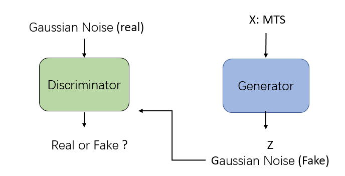
Figure 1: The general framework of Gaussian GANs.

In this paper, we address the visualization problem by introducing a transformation function using GANs instead of following the dimension reduction or down-streaming task verification. Inspired by the uniform transformation theory rosenblatt1952remarks and Kolmogorov–Smirnov test justel1997multivariate under the multivariate case, we construct a transformation function that is able to transform target distribution into standard multivariate Gaussian distribution using GANs. (We call this GANs as Gaussian GANs). With the transformation function, various normality tests can be used to evaluate the goodness of generated samples. Formally, denoting $G_{n}()$ as the generator and $D_{n}()$ as the discriminator of the Gaussian GANs, we let MTS, denoted as $\mathbf{X}$, be the input to the generator, and Gaussian noise, denoted as $\mathbf{Z}$ as its output, that is $\mathbf{Z}=G_{n}(\mathbf{X})$. Then, we use $D_{n}()$ to distinguish whether the $Z$ is standard multivariate Gaussian noise or not.

We present two experiments on a real dataset, the UniMiB dataset , to show the effectiveness of our visualization methods. Our results show that the generated MTS are visually acceptable under both normality test using Gaussian distribution and PCA visualization if two datasets come from the same distribution. If two datasets, however, come from different distributions, the generated MTS are visually terrible from the normality test using Gaussian distribution but acceptable from PCA visualization. The Gaussian GANs can be constructed based on most GANs’ architecture, and we expect that it is applicable to other MTS evaluation problems.

2 Related Work

Similarity in MTS In time-series data mining, similarity measures can be classified into four categories, shape-based, edit-based, feature-based, and model-based distances esling2012time . The shape-based distance compares the whole shape of time series sequences and aims to measure the similarity from points to points, such as the Euclidean distance, Dynamic Time Warping (DTW)berndt1994using and Spatial Assembling Distance chen2007spade . The edit-based distances compare the minimum number of operations needed to transform one series into another one. The proper algorithm is the core to the edit-based distances, such as Longest Common SubSequence algorithm das1997finding , Constraint Continuous Editing Distancechhieng2007adaptive If used in measuring similarity between groups, the shape-based distance and the edit-based distance would be computationally expensive, even more than $O(n^{3})$. The feature-based similarity uses constructed statistical features to measure the similarity, such as a likelihood ratio for DFT coefficients janacek2005likelihood , a combination of periodogram and autocorrelation functions vlachos2005periodicity , and copula-based similarity measures safaai2018information . There is plenty of mathematics behind the feature-based similarity compared to the first two methods, but it is a more efficient measure way. Model-based distance methods usually have an assumption that the time series can be well captured by the proposed model, and then estimate the parameters in the model and lastly calculate the distance, such as ARMA model xiong2004time . The disadvantage is the difficulty of verifying the assumptions. Note that the similarity measures can be extended to measure groups although they are formulated in two single time series sequences.

Uniform Transformation The uniform transformation theory provides that there exists a transformation function $F()$ which can transform any distribution into uniform distribution at interval $[0,1]$ rosenblatt1952remarks . With the transformation function, the Kolmogorov–Smirnov test was used to test the divergence of two distributions justel1997multivariate . The $F()$ is the Cumulative Density Function (CDF) of random variables to be transformed. Under the univariate case, any random variable with continuous CDF $F()$ can be transformed into a uniform random variate on the interval $[0,1]$. In higher dimensions, however, it would be computationally expensive or even impossible to estimate the continuous CDF because the probability integral transformation is a much richer tool that is also far less understood genest2001multivariate .

In our work, we model a transformation function $f()$ with regards to Probability Density Function (PDF) instead of CDF $F()$ and thus skip the high dimension’s integration. Meanwhile, we replace the targeted uniformed distribution at interval $[0,1]$ with standard multivariate Gaussian distribution to make the output of $f()$ more statistically reasonable.

3 Background

3.1 Generative Adversarial Networks

Two parts contained in the GANs: Generator (G) and Discriminator (D), and they play the following two-player minimax game with value function V (G, D) gans :

$$\min_{G}\max_{D}V(D,G)=\mathbb{E}_{\mathbf{x}\sim p_{data(\mathbf{x})}}[logD(\mathbf{x})]+\mathbb{E}_{\mathbf{z}\sim p_{N(\mathbf{z})}}[log(1-D(G(\mathbf{z})))]$$ (1)

, where $\mathbf{z}\sim p_{N}(\mathbf{z})$ means the $\mathbf{z}$ is sampled from the Normal distribution, $\mathbf{x}\sim p_{data(\mathbf{x})}$ means the $\mathbf{x}$ is sampled from the real dataset, $G(\mathbf{z})$ is the mapping from Gaussian noise to generated data, and $D(\mathbf{x})$ or $D(G(\mathbf{z}))$ is to tell whether the input data is fake (generated) or real. The Equation. 1 can be reformulated into two circular steps:

$$arg\max_{\theta_{D}} \mathbb{E}_{\mathbf{x}\sim p_{data(\mathbf{x})}}[logD_{\theta_{D}}(\mathbf{x})]+\mathbb{E}_{\mathbf{z}\sim p_{N(\mathbf{z})}}[log(1-D_{\theta_{D}}(G(\mathbf{z})))]$$ (2)

$$arg\min_{\theta_{G}} \mathbb{E}_{\mathbf{z}\sim p_{N(\mathbf{z})}}[log(1-D(G_{\theta_{G}}(\mathbf{z})))]$$

3.2 Problem Description

Given a dataset $\mathbf{X}_{real}=\{\mathbf{x}_{i},i=1,2,\dots,n\}$, generative models attempts to find a fake distribution $p_{fake}(\mathbf{x})$ to approximate the real distribution $p_{real}(\mathbf{x})$. Specifically, GANs trains a generator $G$, $G(\mathbf{z})\sim p_{fake}(\mathbf{x})$, to reduce the divergence between distribution $p_{real}(\mathbf{x})$ and $p_{fake}(\mathbf{x})$ by minimax games. The generated samples set $\mathbf{X}_{fake}$ are obtained from the $G(\mathbf{z})$. The paper’s aim is to find a metrics $M(\mathbf{X}_{fake},\mathbf{X}_{real})$ to visually and numerically and evaluate the quality of generated samples.

4 GaussianGANs

4.1 Gaussian Transformation using GANs

Let us consider a GANs task, mapping the real data into Gaussian noise. The input for generator and discriminator is MTS, the output of generator is Gaussian noise and the output of discriminator is True/False, that is, to train a GANs which transforms the distribution of MTS into standard multivariate Gaussian distribution. The task could be represented by the following assumption,

Assumption 1.

There exists a Gaussian GANs, $G_{n}()$, which is able to map the real data (high dimensions) to Gaussian noise (low dimensions),

$$\mathbf{z}=G_{n}(\mathbf{x}),\;\;\mathbf{z}\sim N(\boldsymbol{0},\mathbf{I}),\;\mathbf{x}\sim f_{real}(\mathbf{x})$$ (3)

, where $\mathbf{x}$ is data sampled from the real dataset $\mathbf{X}_{real}$, and $\mathbf{z}$ is sampled from the standard multivariate Normal distribution. Moreover, the dimension of $X$ is more than that of $Z$.

With the Gaussian generator, the real data in the high dimensions could be transformed into the low dimension Gaussian noise. In other words, the transformed real data could be regarded to be sampled from the standard normal distribution, $G_{n}(\mathbf{x})\sim N(\boldsymbol{0},\mathbf{I})$. If the distribution of fake data (or generated data) is similar to that of real data enough, the transformed fake data should follow the normal distribution, that is, $G_{n}(G(\mathbf{z}))\sim N(\boldsymbol{0},\mathbf{I})$. With a convincing Gaussian generator, $G_{n}()$, we could construct the new dataset as follows to evaluate the quality of the generated data,

Theorem 1.

Given a well-trained generator $G_{n}$, that is $G_{n}(\mathbf{X}_{real})\sim N(\boldsymbol{0},\mathbf{I})$, the dataset $\mathbf{U}=\{u_{k}|k=1,2,...,n\}$ is sampled from the $\chi^{2}(c*s)$ distribution,

$$u_{k}=\sum_{i=1}^{c}\sum_{j=1}^{s}y_{fake,ijk}^{2},\;k=1,2,...,n,$$ (4)

, where $n$ is the number of fake samples, $c$ means the dimensions of time series, $s$ represents the length of time series, $\mathbf{y}_{fake,k}=G_{n}(\mathbf{x}_{fake,k})$, $x_{fake,ijk}$ is the value of the $\mathbf{x}_{fake,k}$ at its location of (i, j).

Note: Theorem.1 provides a sufficient condition but is not necessary. Moreover, the Theorem.1 also applies to the $\mathbf{U}$ computed from $\mathbf{X}_{real}$, because of the hypothesis that both $\mathbf{X}_{real}$ and $\mathbf{X}_{fake}$ come from the same distribution.

The method of evaluating the quality of generated time series is summarized as follows:

• Train a well-performed Gaussian GANs;

• Evaluate the quality of generated MTS with our proposed metrics and visualization.

The section 4.2provides how to train the Gaussian GANs; the section 4.3 4.4 are the proposed metric and visualization method.

4.2 General Architecture

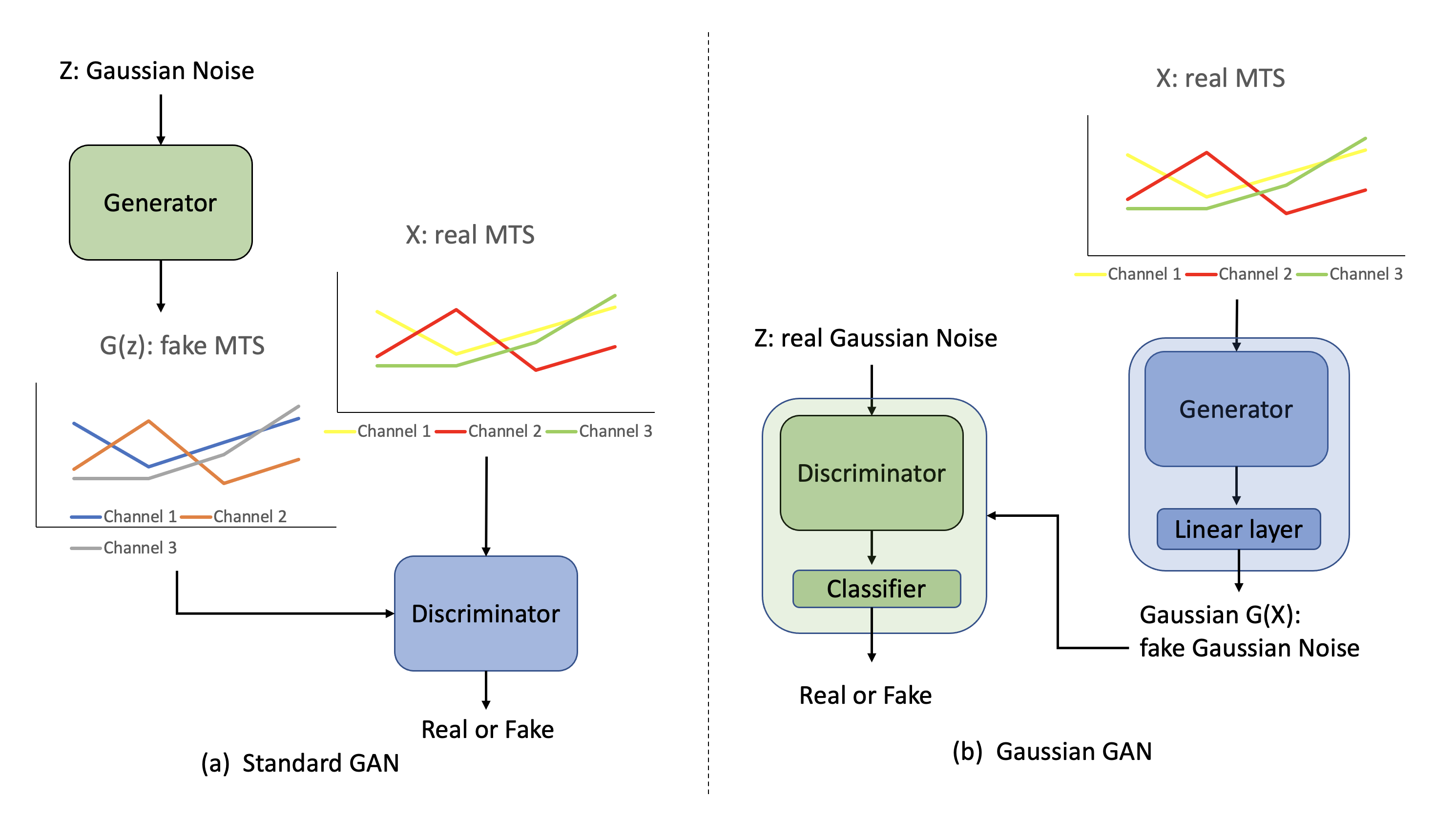
Figure 2: GaussianGANs architecture. The (a) is a standard architecture for GANs, the input to the generator is Gaussian noise and the output is generated MTS; the input to the discriminator is the real and fake MTS and the output is a scalar (real or fake). The (b) is the general framework for Gaussian GANs, where there are only 2 modifications compared to the standard architecture

There is no specific architecture for Gaussian GANs but it has a general architecture in which different models have their own different architectures. That is because the Gaussian GANs can be used in most scenarios of MTS generation tasks when the following two points are satisfied: (1) the generative model is GANs and (2) the generator and discriminator use the same blocks in their own architecture. In figure 2, the (a) contains a standard architecture for GANs, the input to the generator is Gaussian noise and the output is generated MTS; the input to the discriminator is the real and fake MTS and the output is a scalar (real or fake). The (b) is the general framework to Gaussian GANs, where there are only 2 modifications compared to the standard architecture,

• The generator of the Gaussian GANs uses the discriminator of the standard GANs, but changes the output from a scalar to the dimension of Gaussian noise at the last layer;

• The discriminator of the Gaussian GANs uses the generator of the standard GANs, but changes the output from the dimension of MTS to the dimension of Gaussian noise at the last layer;

4.3 Normality Metrics - Sufficient and Necessary

As Assumption 1 indicates, the fake data (or real data) transformed by Gaussian GANs, $G_{n}(\mathbf{X}_{fake})$, follows the standard multivariate normal distribution if the $G_{n}()$ has been well trained. Considering the properties of standard multivariate normal distribution, it would be simple and efficient to use heatmap for correlation matrix and univariate normality test to examine the quality of generated data. Because in the multivariate normal distribution, the independence among features (random variables) would be equivalent to that of the correlation between any two features is equal to 0. Moreover, with the independence among features, the multivariate normality test (difficult and computationally expensive) could be replaced by a univariate normality test (simple and computationally efficient).

Correlation heatmap. Let $\mathbf{Y}=G_{n}(\mathbf{X}_{fake})$, (or $\mathbf{Y}=G_{n}(\mathbf{X}_{real})$). The correlation matrix, $\mathbf{R}=\{r_{ij}\}_{p\times p}$, for transformed data could be estimated by following estimation method,

$$r_{ij}=\frac{\mathbf{y}_{i}^{T}\times\mathbf{y}_{j}}{||\mathbf{y}_{i}|||\mathbf{y}_{j}||},i,j=1,2,..,p,$$ (5)

where the $\times$ means the dot product for two vectors, and the ||$\mathbf{y}_{i}$|| is the L1 norm for vector $\mathbf{y}_{i}$. If the a well trained GANs satisfies the Assumption 1, the values off the diagonal should be close to 0 and the values alone the diagonal should be close to 1.

Normality test. Shapiro-Wilk test shapiro1965analysis and D’Agostino’s K-squared test normaltest are used to identify whether the transformed data follows the normal distribution. The Shapiro-Wilk test statistics is,

$$W=\frac{(\sum_{i=1}^{n}a_{i}x_{(i)})^{2}}{\sum_{i=1}^{n}(x_{i}-\bar{x})^{2}}$$ (6)

$$(a_{1},...,a_{n})=\frac{\mathbf{m}^{T}V^{-1}}{C}$$ (7)

$$C=||V^{-1}\mathbf{m}||=(\mathbf{m}^{T}V^{-1}V^{-1}\mathbf{m})^{\frac{1}{2}},$$ (8)

where $W$ is the Shapiro-Wilk test statistics, $x_{(i)}$ is order statistics, which is different than the $x_{i}$. $\bar{x}=\frac{\sum_{i=1}^{n}x_{i}}{n}$, $\mathbf{a}$ is weighted coefficient determined by both standard normal distribution and the dataset. $\mathbf{m}=(m_{1},m_{2},...,m_{n})^{T}=(\mathbb{E}x^{\prime}_{(1)},\mathbb{E}x^{\prime}_{(2)},...,\mathbb{E}x^{\prime}_{(n)})=\mathbb{E}(\mathbf{x^{\prime}})$, where $x^{\prime}_{(i)}$ is the identically and independently distributed random variables which follow the standard normal distribution. $V$ is covariance matrix of those normal order statistics shapiro1965analysis . D’Agostino’s K-squared statistics proposed the revised skewness and kurtosis to make the original skewness and kurtosis converge as fast as possible. The details of the statistics are contained in the normaltest normaltest2

Note: the ideal quality of a generated dataset should have a small p-value and correlation matrix as close as to the identity matrix.

4.4 Visualization - Sufficient

Let’s consider the hypothesis in the Assumption 1 that the Gaussian GANs and the generative model is well trained, then the transformed dataset (generated or real dataset) would be samples from $\chi^{2}(c\times s)$ distribution according to the Theorem.1. Thus, both of the $\mathbf{u}_{real}=(u_{real,1},...,u_{real,n})$ and $\mathbf{u}_{fake}=(u_{fake,1},...,u_{fake,n})$ could visualized through QQ plot, which is used to identify whether the hypothesis is true or not. But $\chi^{2}$ Visualization is not a necessary condition as normality metrics in Section 4.3 to test the quality of the generated data. The simplicity and efficiency, however, is the advantage of $\chi^{2}$ Visualization.

5 Experiments

5.1 Transformer GaussianGANs

To illustrate how our method works, the transformer-based time series GANs (ttsGANs) ttsgan is used because of its better results under PCA visualizations. In addition, the model is trained on the 1 GV100 32G with 4 hours. There are merely 2 modifications for the corresponding Gaussian GANs based on the ttsGANs. In the figure 3, the ttsGANs is light blue shadowed, and its corresponding Gaussian GANs is light green shadowed. The 2 modifications are shadowed with dark blue and dark green separately: the architecture switch between generator and discriminator and their output layer, specifically,

• The generator in Gaussian GANs uses the discriminator architecture in the ttsGANs; and the discriminator in Gaussian GANs uses the generator architecture in the ttsGANs;

• The output layers of generator in Gaussian GANs and ttsGANs are both Conv2D channels reduction; and the output layers of generator in Gaussian GANs and ttsGANs are both classification head.

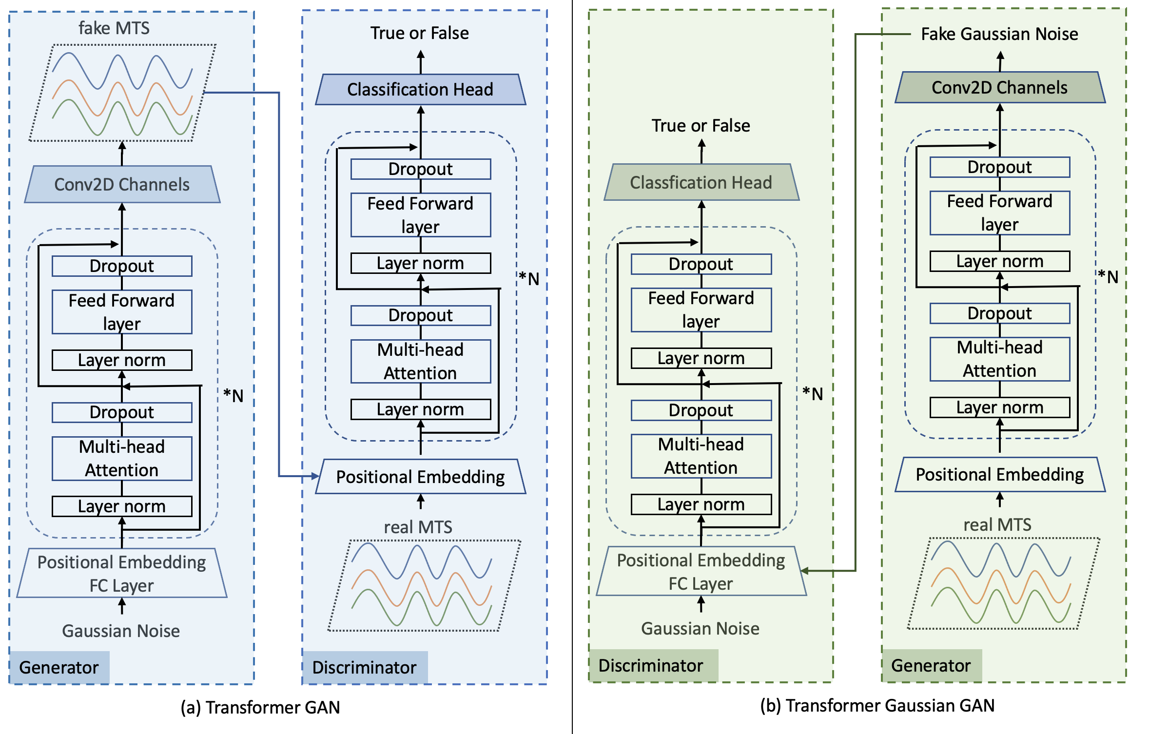
Figure 3: Gaussian GAN based on transformer-based time series GANs. (a) the ttsGANs is light blue shadowed, and (b) its corresponding Gaussian GANs is light green shadowed. The 2 modifications are shadowed with dark blue and dark green separately, that is, the architecture switch between generator and discriminator and their output layer.

5.2 Datasets

We adopt the same datasets used in the ttsGANs paper ttsgan , the UniMiB dataset dataset , where two categories are selected: Jumping and Running because the effect of ttsGAN is different under the two categories. Thus, it can be observed how the normality metrics and $\chi^{2}$ visualization would change while results change from good to bad. The sample size for the two classes in the training dataset is 600 and 1572 respectively, that in testing dataset is 167 and 416 respectively. Both of the classes have 150 timestamps and 3 channels. Additionally, all of the recordings are channel-wisely normalized to a mean of 0 and a variance of 1.

5.3 Results

Training Gaussian GANs In order to select the best Gaussian GANs during the training epochs, a comprehensive metric is designed:

$$S =S_{1}+S_{2}+S_{3},\;\;\;$$ (9)

$$S_{1} =\frac{1}{n\times c}\sum_{j=1}^{c}|\sum_{i=1}^{n}x_{ij}|+\frac{1}{c}\sum_{j=1}^{c}(|\frac{1}{n}\sum_{i=1}^{n}(x_{ij}-\bar{x}_{i\cdot})^{2}-1|)^{\frac{1}{2}}$$ (10)

$$S_{2} =\frac{1}{c\times c}sum(|\mathbf{r}-\mathbf{I}|)$$ (11)

$$S_{3} =\frac{1}{n}\sum_{i=1}^{n}S_{3i}$$ (12)

$$S_{3i} =\begin{cases}1,&p_{i1}>0.9\;and\;p_{i2}>0.9\\ 0,&otherwise\\ \end{cases},$$ (13)

where c is the number of dimensions of the multivariate normal distribution; and n is the number of samples. S is constructed by three features of the dataset: $S_{1}$ moment distance, $S_{2}$ correlation matrix distance, and $S_{3}$ normality distance. In detail, $S_{1}$ is composed of the mean and variance of the dataset; in the $S_{2}$, the $sum$ means the sum of all points in the matrix, which represents the distance of two matrices; $S_{3}$ is determined by the p-values of two normality test, which represents the percentage of how many dimensions that do not follow a normal distribution.

For the Running dataset, the training process of Gaussian GANs at epochs 0, 400 and 630 is shown in figure 4. At epoch 0, it is seen that the generated MTS cannot cover the region of the real dataset under PCA visualization, although the correlation matrix is close to the identity matrix with a small value of $S3$ and the QQ plot is almost a straight line. It is because the output of the neural network is close to white noise when the whole network has not been trained, under which circumstance any type of dataset could be transformed into a normal distribution. That is not what we expected because Gaussian GANs is aimed to transform the dataset from a certain distribution into samples from the standard multivariate normal distribution. (, which is discussed in Section 6).

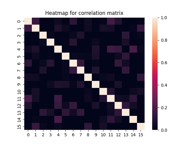
(a) Heatmap: epoch 0 ($S_{3}=0.25$)

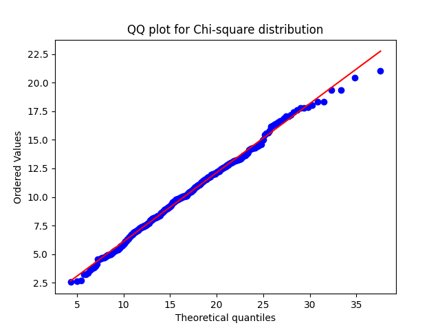
(b) QQ plot: epoch 0

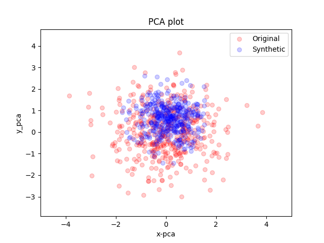
(c) PCA visualization: epoch 0

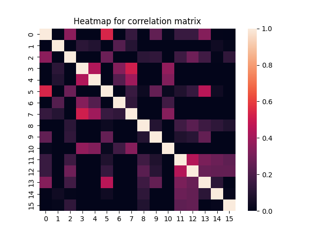
(d) Heatmap: epoch 400 ($S_{3}=0.125$)

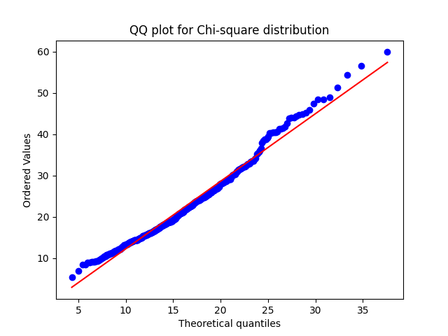
(e) QQ plot: epoch 400

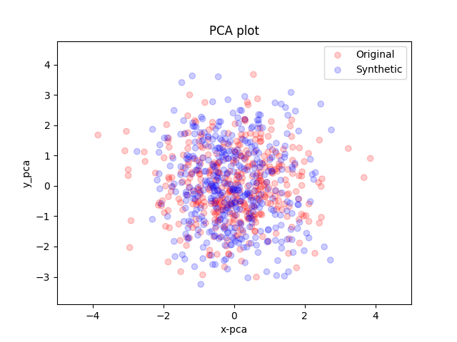
(f) PCA visualization: epoch 400

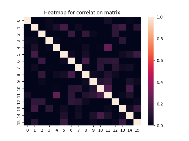
(g) Epoch 630 ($\mathbf{S_{3}=0.1875}$)

(h) QQ plot: epoch 630

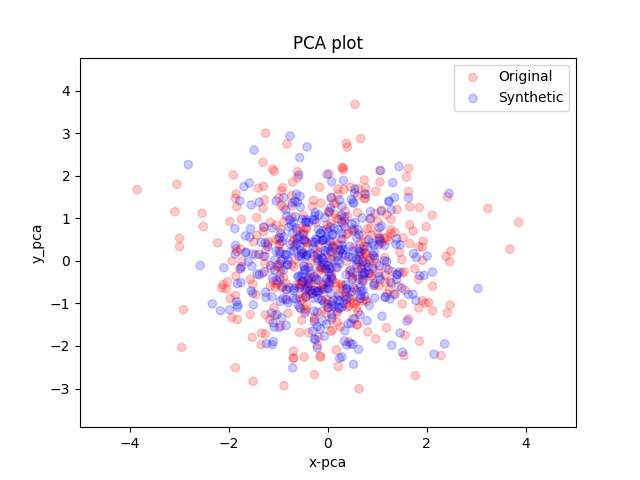
(i) PCA visualization: epoch 630

Figure 4: Running dataset for Gaussian GANs. At epoch 0, the generated MTS cannot cover the region of the real dataset under PCA visualization, in spite of a good normality test and $\chi^{2}$ visualization. Because the output of neural network is close to white noise when the whole network has not been trained. In the following training epochs, the correlation matrix is transitioning to the identity matrix with a small $S_{3}$ values, moreover, the QQ plot is almost a straight line, and the generated MTS and the real MTS overlap under PCA visualization. In addition, the best Gaussian GANs is in bold with $S=4.034$

In the following training epochs, we could see at epoch 400 that the correlation matrix is not close to the identity matrix, but $S_{3}$ = 0.125 represents that 87.5% dimensions follows normal distribution, which indicates the generated data are not sampled from the real distribution. PCA visualization and QQ plot, however, indicates a completely different conclusion based on that the generated MTS and the real MTS overlap under most of area and QQ plot is transitioning to a straight line. It is because normality test using Gaussian GANs is able to retain more information than PCA and QQ plot in theory. According to the comprehensive metric $S$, the best Gaussian GANs is in bold in the figure 4 (g,h,i) with the value of 4.034. Moreover, it is clear that Gaussian GANs well pass the normality test, QQ plot and PCA visualization. Therefore, we argue that Gaussian GANs successfully transform the Jumping dataset from its distribution into white noise from the standard multivariate normal distribution.

Evaluating quality of generated MTS

With the best Gaussian GANs, the training process could be monitored, that is to say, the quality of the generative MTS could be visualized at every training process epoch.

Firstly, it is necessary to verify that the Gaussian GANs really works by feeding the test dataset into the Gaussian GANs, and the results is shown in figure 5 and it indicates that the testing dataset and training dataset comes from the same distribution. From the perspective of normality test, the heatmap is close to identity matrix and $S_{3}=0.06$ close to 0, and thus the assumption 1 is satisfied. The line is nearly straight, which satisfies Theorem 1. Moreover, the testing and training dataset almost overlaps in their regions.

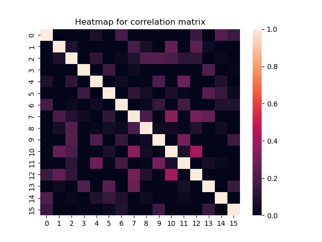
(a) Heatmap ($S_{3}=0.06$)

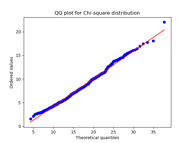
(b) QQ plot

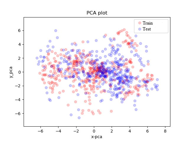
(c) PCA visualization

Figure 5: Verification for Gaussian GANs by feeding the test dataset.

Secondly, ttsGANs is trained to generate MTS and then use Gaussian GANs to evaluate the quality of the generated MTS. The results of the Running dataset is shown in figure 6, from which PCA visualization and QQ plot point to a good quality of the generated dataset. The normality test using Gaussian GANs, however, leads to the opposite side (correlation matrix is not close to identity matrix), because the normality test can capture more information between two groups, which experimentally signifies that normality test using Gaussian GANs is more robust than $\chi^{2}$ and PCA visualization.

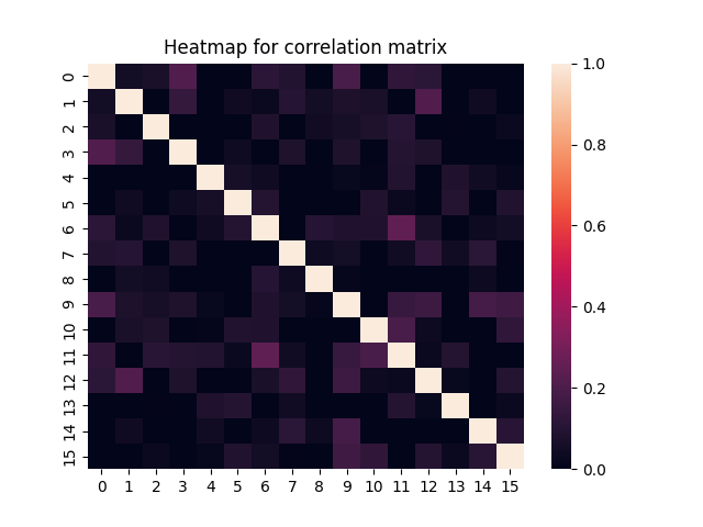
(a) Heatmap: epoch 0 ($S_{3}=0.0625$)

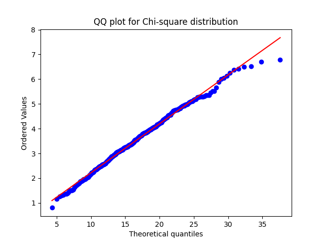
(b) QQ plot: epoch 0

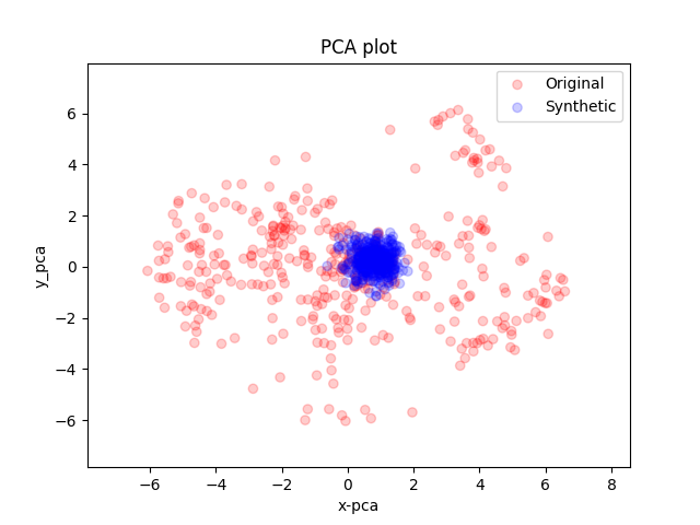
(c) PCA visualization: epoch 0

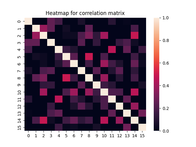
(d) Heatmap: epoch 1000 ($S_{3}=0.125$)

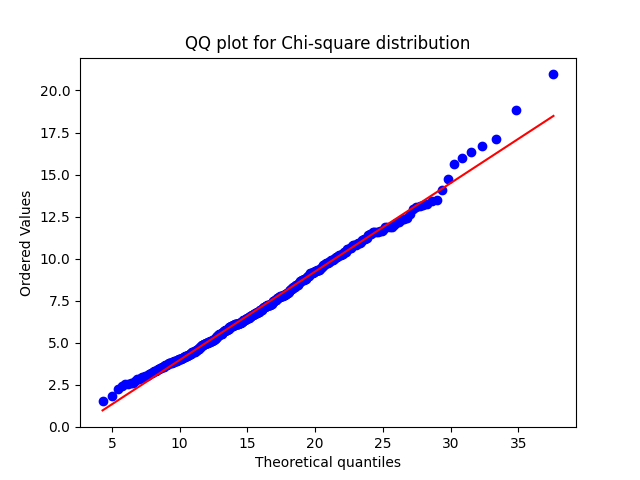
(e) QQ plot: epoch 1000

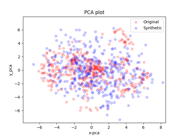
(f) PCA visualization: epoch 1000

Figure 6: Running dataset training process. At the epoch 1000, the good performance under PCA visualization is reflected on QQ plot, but not for heatmap, because the heatmap retains more information than the PCA does. That is, the generated MTS is not as good as PCA visualization shows.

6 Limitations

The normality test using Gaussian GANs is an effective tool to verify whether the generated data and real data come from the same distribution. However, there are some points that need to be address in future work:

• Why does the normality test using Gaussian GANs fails at the initial training stage and how to fix it. From the perspective of experiments, the output of the generator in the Gaussian GANs is nearly white noise at the initial training epoch, thus making the normality test for the multivariate normal distribution fail.

• Is there an effective and simple method which is necessary and sufficient condition for assumption 1 to test the normality. Normality test using Gaussian in the Assumption 1 is compound, where both correlation matrix and $S_{3}$ should be measured simultaneously. The QQ plot, on the other hand, is not a necessary condition for assumption 1.

• If there is not such a GANs architecture when generating new data, such as the VAE, flow-based generative model, or statistical models, is it possible to establish an architecture to evaluate the quality of generated data.

7 Conclusion

We theoretically and experimentally discussed the effectiveness of our proposed evaluation methods, the normality test using Gaussian GANs, which captures more information than PCA does. Importantly, the Gaussian GANs is the general framework that can be easily constructed from most types of GANs under the MTS task. Moreover, in order to simplify the normality test using Gaussian GANs, the QQ-plot in theorem.1 is attempted as a tentative exploration.

Appendix A Appendix - Gaussian GANs over Jumping dataset

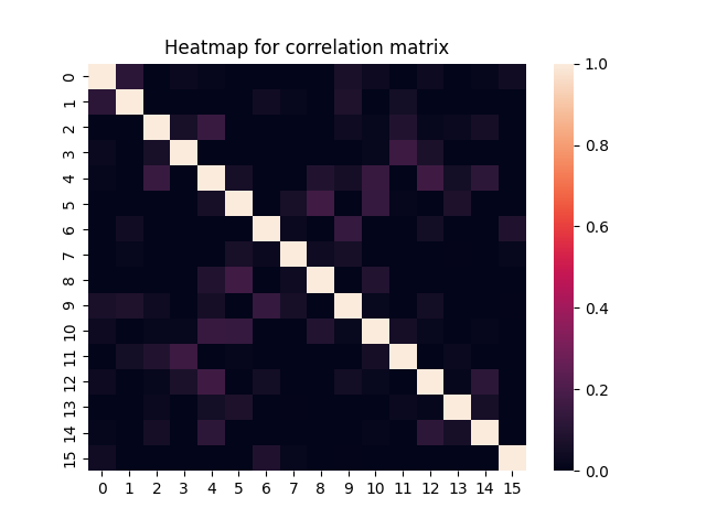
(a) Heatmap: epoch 0 ($S_{3}=0.125$)

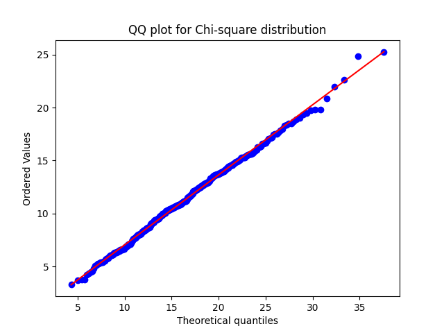
(b) QQ plot: epoch 0

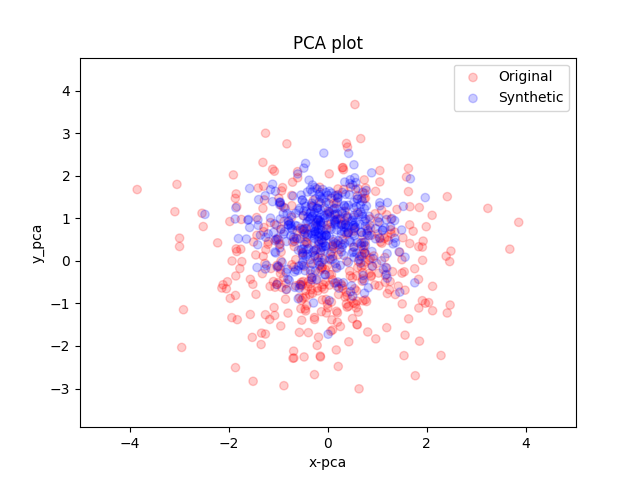
(c) PCA visualization: epoch 0

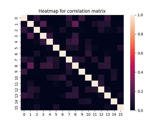
(d) Heatmap: epoch 560 ($S_{3}=0.375$)

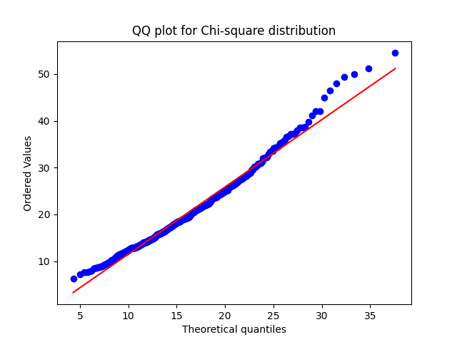
(e) QQ plot: epoch 560

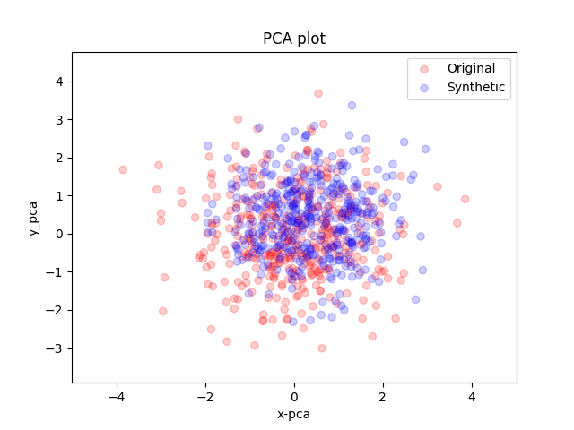
(f) PCA visualization: epoch 560

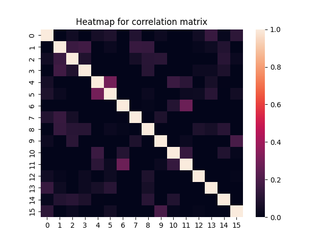
(g) Epoch 930 ($\mathbf{S_{3}=0.125}$)

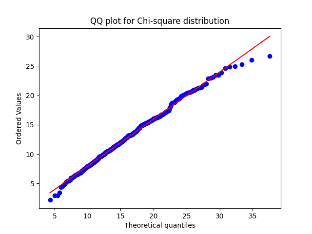
(h) QQ plot: epoch 930

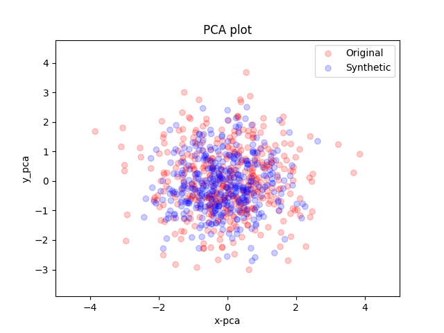
(i) PCA visualization: epoch 930

Figure 7: Jumping dataset for Gaussian GANs.

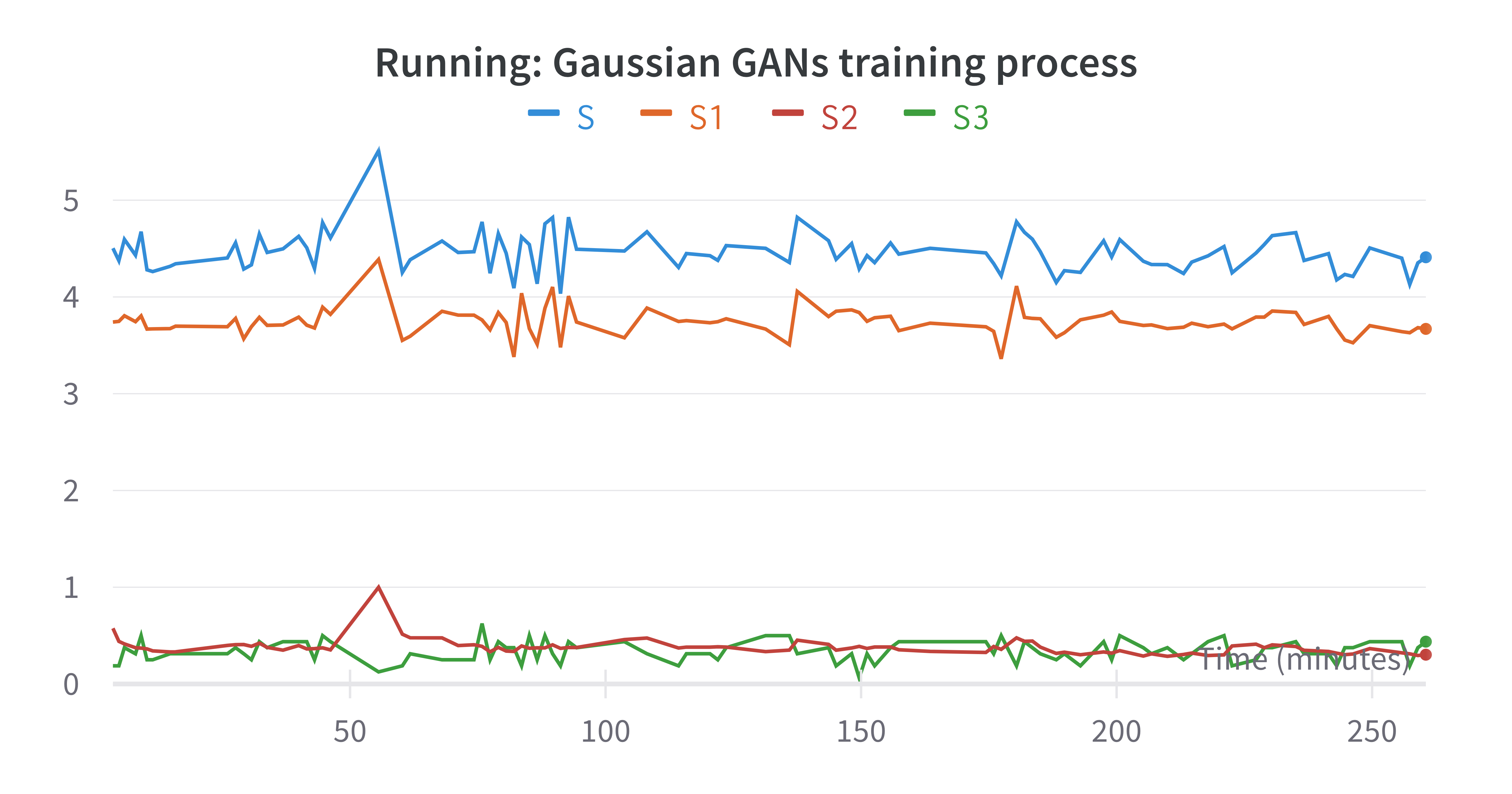
(a) Gaussian GANs for Running dataset

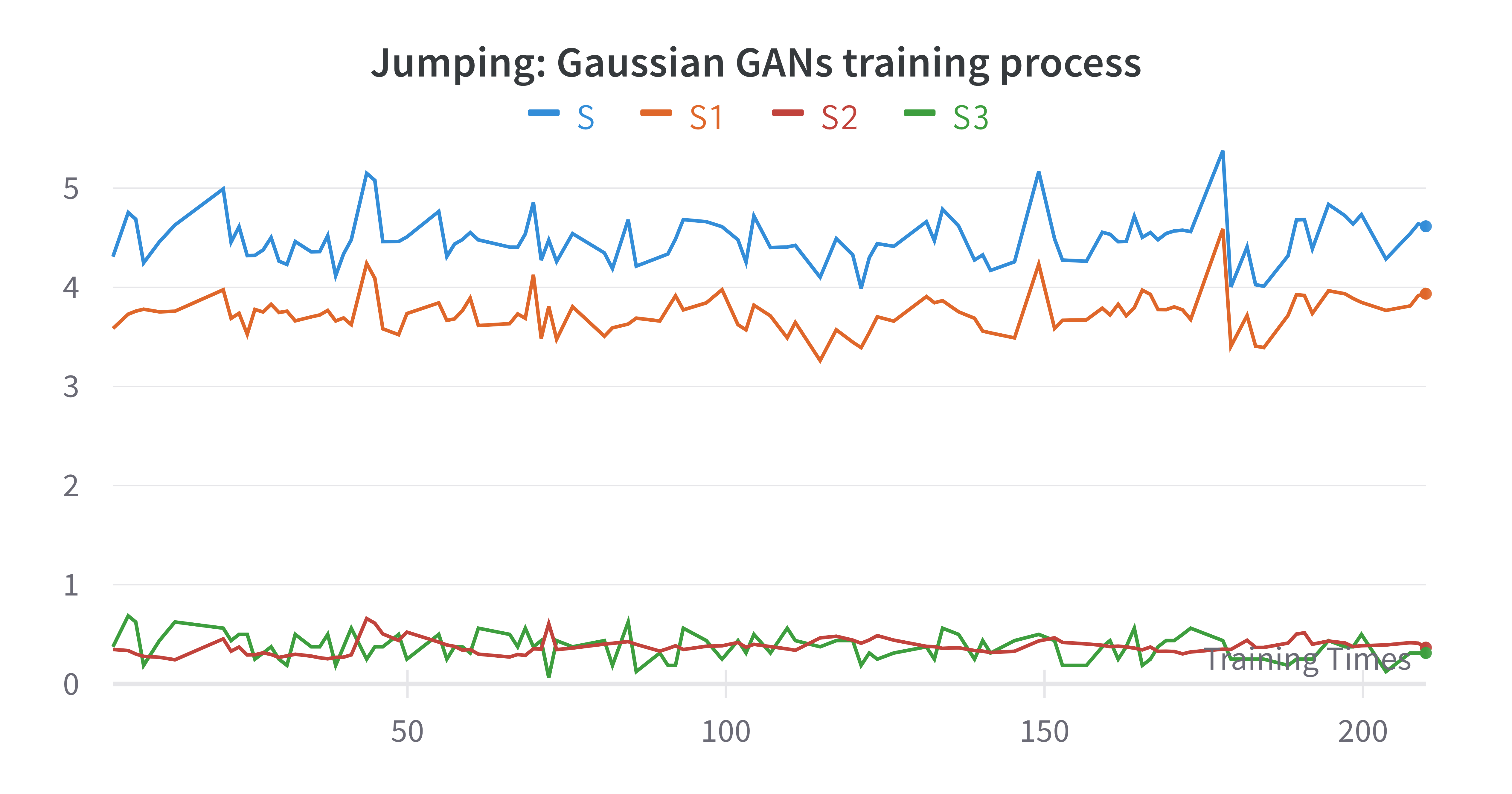
(b) Gaussian GANs for Jumping dataset

Figure 8: Gaussian GANs training process: $S,S_{1},S_{2},S_{3}$. The S is largely determined by the $S_{1}$.

At epoch 0, the generated MTS cannot cover the region of the real dataset under PCA visualization, although the generated data passed the normality test and $\chi^{2}$ visualization under Gaussian GANs. At epoch 560, the generated data is poor because of the normality test (large $S_{3}$ values), $\chi^{2}$ visualization (tail shift), and PCA visualization (not totally overlap). At epoch 930, the best Gaussian GANs is identified in bold with $S=3.868$, with normality test (correlation matrix close to identity matrix and a small $S_{3}$ values), QQ plot (almost a straight line), PCA visualization (totally overlap).

Appendix B Appendix - Evaluation over Jumping Dataset

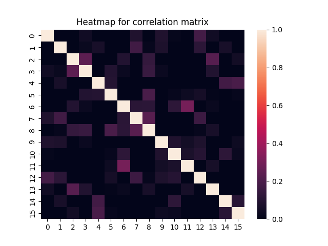
(a) Heatmap: epoch 0

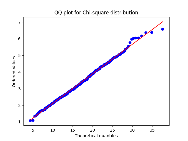
(b) QQ plot: epoch 0

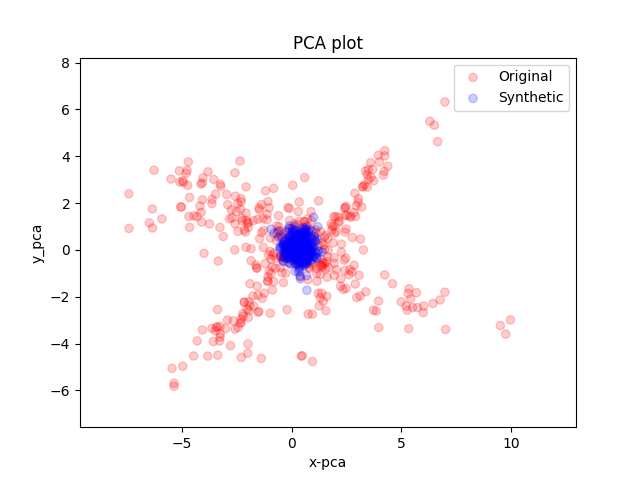
(c) PCA visualization: epoch 0

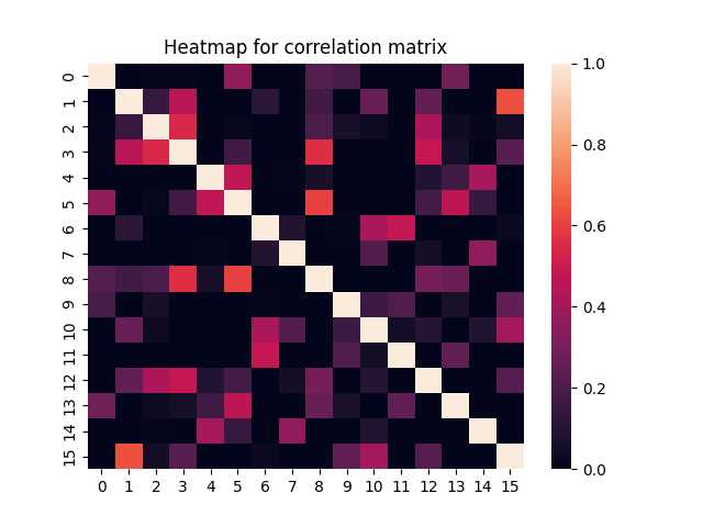
(d) Heatmap: epoch 280

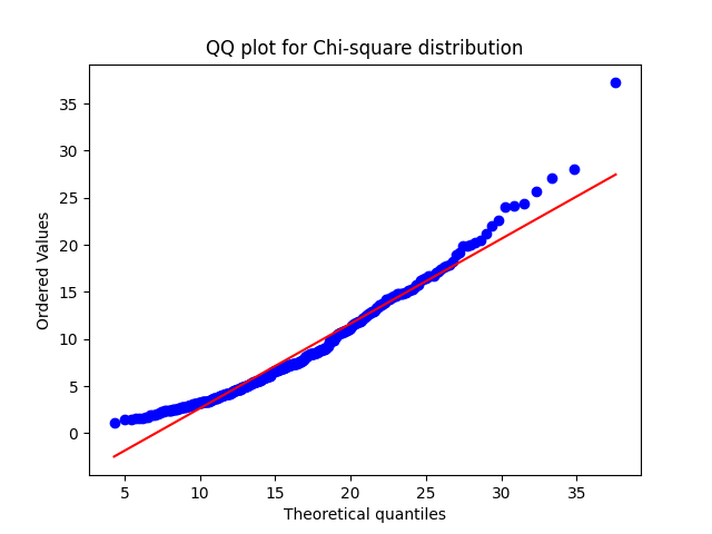
(e) QQ plot: epoch 280

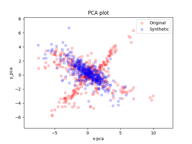
(f) PCA visualization: epoch 280

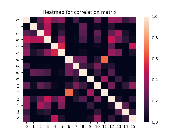
(g) Heatmap: epoch 1580

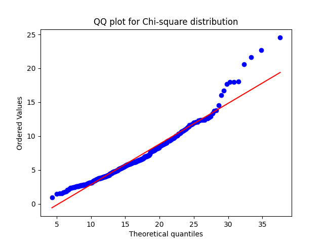
(h) QQ plot: epoch 1580

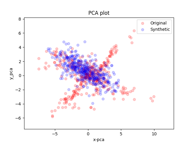
(i) PCA visualization: epoch 1580

Figure 9: Jumping dataset for ttsGANs. At the epoch 280 and 1580, the poor performance under PCA visualization is reflected on the heatmap and QQ plot.

In the figure 9 (Jumping dataset), it is seen that the normality test and QQ plot using Gaussian GANs almost reaches the ideal state but fails under PCA visualization at the epoch = 0. We argue that the mismatch between assumption 1 and PCA visualization is caused by the slight robustness of Gaussian GANs to white noise (discussed in Section. 6). At epoch 280 and 1580, the QQ plot cannot reach a straight diagonal line and heatmap cannot be as close as to the identity matrix when the generated MTS fails to cover the region of the real MTS under PCA visualization. Moreover, in the figure 8 (a), the $S_{3}$ have large values, which means that nearly half of the dimensions of the transformed MTS do not come from the Gaussian distribution. In other words, the normality test and QQ plot would not manifest a good results if two dataset cannot overlap under the PCA visualization.

References

- [1] Francis J Anscombe and William J Glynn. Distribution of the kurtosis statistic b2 for normal samples. Biometrika, 70(1):227–234, 1983.
- [2] Donald J Berndt and James Clifford. Using dynamic time warping to find patterns in time series. In KDD workshop, volume 10, pages 359–370. Seattle, WA, USA:, 1994.
- [3] Yueguo Chen, Mario A Nascimento, Beng Chin Ooi, and Anthony KH Tung. Spade: On shape-based pattern detection in streaming time series. In 2007 IEEE 23rd international conference on data engineering, pages 786–795. IEEE, 2007.
- [4] Van M Chhieng and Raymond K Wong. Adaptive distance measurement for time series databases. In International Conference on Database Systems for Advanced Applications, pages 598–610. Springer, 2007.
- [5] RALPH D’AGOSTINO and Egon S Pearson. Tests for departure from normality. empirical results for the distributions of b2 and b. Biometrika, 60(3):613–622, 1973.
- [6] Gautam Das, Dimitrios Gunopulos, and Heikki Mannila. Finding similar time series. In European Symposium on Principles of Data Mining and Knowledge Discovery, pages 88–100. Springer, 1997.
- [7] Hao-Wen Dong, Wen-Yi Hsiao, Li-Chia Yang, and Yi-Hsuan Yang. Musegan: Multi-track sequential generative adversarial networks for symbolic music generation and accompaniment. In Proceedings of the AAAI Conference on Artificial Intelligence, volume 32, 2018.
- [8] Philippe Esling and Carlos Agon. Time-series data mining. ACM Computing Surveys (CSUR), 45(1):1–34, 2012.
- [9] Christian Genest and Louis-Paul Rivest. On the multivariate probability integral transformation. Statistics & probability letters, 53(4):391–399, 2001.
- [10] Ian Goodfellow, Jean Pouget-Abadie, Mehdi Mirza, Bing Xu, David Warde-Farley, Sherjil Ozair, Aaron Courville, and Yoshua Bengio. Generative adversarial nets. Advances in neural information processing systems, 27, 2014.
- [11] Narit Hnoohom, Sakorn Mekruksavanich, and Anuchit Jitpattanakul. Human activity recognition using triaxial acceleration data from smartphone and ensemble learning. In 2017 13th international conference on signal-image Technology & Internet-Based Systems (SITIS), pages 408–412. IEEE, 2017.
- [12] Gareth J Janacek, Anthony J Bagnall, and Michael Powell. A likelihood ratio distance measure for the similarity between the fourier transform of time series. In Pacific-Asia Conference on Knowledge Discovery and Data Mining, pages 737–743. Springer, 2005.
- [13] Ana Justel, Daniel Peña, and Rubén Zamar. A multivariate kolmogorov-smirnov test of goodness of fit. Statistics & Probability Letters, 35(3):251–259, 1997.
- [14] Tero Karras, Miika Aittala, Samuli Laine, Erik Härkönen, Janne Hellsten, Jaakko Lehtinen, and Timo Aila. Alias-free generative adversarial networks. Advances in Neural Information Processing Systems, 34, 2021.
- [15] Xiaomin Li, Vangelis Metsis, Huangyingrui Wang, and Anne Hee Hiong Ngu. TTS-GAN: A Transformer-based Time-Series Generative Adversarial Network. arXiv preprint arXiv:2202.02691, 2022.
- [16] Qi Mao, Hsin-Ying Lee, Hung-Yu Tseng, Siwei Ma, and Ming-Hsuan Yang. Mode seeking generative adversarial networks for diverse image synthesis. In 2019 IEEE/CVF Conference on Computer Vision and Pattern Recognition (CVPR), pages 1429–1437. IEEE Computer Society, 2019.
- [17] Jin-Hong Park, TN Sriram, and Xiangrong Yin. Dimension reduction in time series. Statistica Sinica, pages 747–770, 2010.
- [18] Daniel Pena and Pilar Poncela. Dimension reduction in multivariate time series. In Advances in distribution theory, order statistics, and inference, pages 433–458. Springer, 2006.
- [19] Murray Rosenblatt. Remarks on a multivariate transformation. The annals of mathematical statistics, 23(3):470–472, 1952.
- [20] Houman Safaai, Arno Onken, Christopher D Harvey, and Stefano Panzeri. Information estimation using nonparametric copulas. Physical Review E, 98(5):053302, 2018.
- [21] Samuel Sanford Shapiro and Martin B Wilk. An analysis of variance test for normality (complete samples). Biometrika, 52(3/4):591–611, 1965.
- [22] Michail Vlachos, Philip Yu, and Vittorio Castelli. On periodicity detection and structural periodic similarity. In Proceedings of the 2005 SIAM international conference on data mining, pages 449–460. SIAM, 2005.
- [23] Yimin Xiong and Dit-Yan Yeung. Time series clustering with arma mixtures. Pattern Recognition, 37(8):1675–1689, 2004.
- [24] Jinsung Yoon, Daniel Jarrett, and Mihaela Van der Schaar. Time-series generative adversarial networks. Advances in Neural Information Processing Systems, 32, 2019.