Modelling multivariate extreme value distributions via Markov trees

Abstract

Multivariate extreme value distributions are a common choice for modelling multivariate extremes. In high dimensions, however, the construction of flexible and parsimonious models is challenging. We propose to combine bivariate extreme value distributions into a Markov random field with respect to a tree. Although in general not an extreme value distribution itself, this Markov tree is attracted by a multivariate extreme value distribution. The latter serves as a tree-based approximation to an unknown extreme value distribution with the given bivariate distributions as margins. Given data, we learn an appropriate tree structure by Prim’s algorithm with estimated pairwise upper tail dependence coefficients or Kendall’s tau values as edge weights. The distributions of pairs of connected variables can be fitted in various ways. The resulting tree-structured extreme value distribution allows for inference on rare event probabilities, as illustrated on river discharge data from the upper Danube basin.

Keywords.  Kendall’s tau; Markov tree; Multivariate extreme value distribution; Prim’s algorithm; probabilistic graphical model; rare event; tail dependence

1 Introduction

The modelling of tail dependence and extreme events has become a statistical problem of great interest. Through asymptotic theory, extreme value theory postulates models for sample extremes (extreme value distributions) and excesses over high thresholds (generalized Pareto distributions), both univariate and multivariate. Fields of application include meteorology and climatology (heat waves, wind storms, floods), finance (stock market crashes), reinsurance (large claims), and machine learning (anomaly detection). Text-book treatments can be found in Coles, (2001), Beirlant et al., (2004) and de Haan & Ferreira, (2006), while Davison & Huser, (2015) provides a more recent survey of the field.

Multivariate extreme value distributions arise as the possible limiting distributions of normalized component-wise maxima of independent copies of a random vector. Their construction, however, is not straightforward because of their complicated dependence structure. Non-parametric inference on multivariate extreme value distributions is usually performed in terms of dependence functions such as the angular or spectral measure (Einmahl et al.,, 2001; Einmahl & Segers,, 2009), the Pickands dependence function (Deheuvels,, 1991) and the stable tail dependence function (Huang,, 1992; Drees & Huang,, 1998). Early reviews of parametric models can be found in Coles & Tawn, (1991), Kotz & Nadarajah, (2000, Chapter 3), and Beirlant et al., (2004, Chapter 9). Well-known parametric models include the logistic and negative logistic families (Gumbel,, 1960; Tawn,, 1990), the Hüsler–Reiss model (Hüsler & Reiss,, 1989), mixtures of Dirichlet distributions (Boldi & Davison,, 2007), the pairwise beta distribution (Cooley et al.,, 2010), max-linear factor models (Einmahl et al.,, 2012), the extremal t process (Davison et al.,, 2012), and models based on Bernstein polynomials (Hanson et al.,, 2017). Some generic construction principles yielding known and new examples are proposed in Ballani & Schlather, (2011) and Kiriliouk et al., (2019). Although these methods perform quite well and have reasonable efficiency in low and moderate dimensions, their application in higher dimensions remains challenging stemming from the potentially complex dependence structure of multivariate extreme value distributions, computational challenges, and the need to balance flexibility with parsimony.

Graphical models represent relatively simple probabilistic structures and are a popular way to model multivariate distributions in a sparse way. Lately, the intersection of extreme value theory and graphical models has attracted quite some attention. Gissibl & Klüppelberg, (2018) introduced max-linear models on directed acyclic graphs, whose dependence structures were further investigated in Gissibl et al., (2018). Segers, (2020) studied the limit theory of extremes of regularly varying Markov trees, with applications to structured Hüsler–Reiss distributions in Asenova et al., (2021) and with extensions to Markov random fields on block graphs in Asenova & Segers, (2021). In parallel, Engelke & Hitz, (2020) proposed a way to factor the density of multivariate generalized Pareto distribution on graphs through a variation on the Hammersley–Clifford theorem related to a kind of redefined conditional independence, followed by Engelke & Volgushev, (2020), who studied a data-driven methodology of identifying the underlying graphical structures for such a factorization. An illuminating review of sparse models for multivariate extremes is given in Engelke & Ivanovs, (2021).

The goal of this paper is to approximate a potentially unknown multivariate extreme value distribution by another multivariate extreme value distribution constructed from a Markov random field with respect to a tree, or Markov tree in short. As special cases of graphical models, Markov trees have simple and tractable structures. The conditional independence relations they satisfy are equivalent to a certain factorization of their joint distribution and eventually lead to an effective dimension reduction. The application of Markov trees in the modelling of multivariate probability distribution goes back to the seminal paper by Chow & Liu, (1968), who approximate a $d$-dimensional discrete distribution by a product of pairwise distributions linked up by a tree. It was demonstrated that in many cases, this method provides a reasonable approximation to the full distribution, capturing at least the marginal distributions and some important features of the joint dependence structure. The idea remains attractive in modern practice. In Horváth et al., (2020), for instance, such Markov tree approximations are used in the context of anomaly detection in machine learning.

A Markov tree involves a set of conditional independence relations between random variables. However, Papastathopoulos & Strokorb, (2016) have shown that for a max-stable random vector with positive continuous density, conditional independence of two random variables given the other ones implies unconditional independence of the two variables. Except for trivial cases, a random vector with a multivariate extreme value distribution and a continuous density can therefore not satisfy any conditional independence relations. Hence, the method of Chow & Liu, (1968) cannot be applied directly to multivariate extreme value distributions. Still, Engelke & Volgushev, (2020) and Segers, (2020) demonstrated that conditional independence relations can be incorporated into distributions of multivariate extremes through the lens of excesses over high thresholds. Based on these findings, we propose a method based on graphical models that consists of merging bivariate extreme value distributions along a tree.

Given a multivariate extreme value distribution and a tree on the set of variables, we construct a Markov tree by letting each connected pair of variables have the same distribution as the corresponding bivariate margin of the extreme value distribution. The Markov tree constructed in this way is shown to belong to the domain of attraction of another extreme value distribution. This second multivariate extreme value distribution serves as a tree-based approximation to the first one, fully determined by the tree structure and certain bivariate margins. Explicit expressions of such a tree-structured multivariate extreme value distribution (see Definition 2.2 below) are derived from those of joint tails of Markov trees.

In practice, the true extreme value distribution is unknown and needs to be estimated from the data. To do so, we implement a three-step procedure: (1) Select the maximum dependence tree which has the maximal sum of edge weights, taken as the pairwise estimates of the upper tail dependence coefficient $\lambda$ or Kendall’s $\tau$; (2) Estimate the dependence structures of all the pairs of adjacent variables on the maximum dependence tree; (3) Measure the goodness-of-fit of the constructed model by comparing the distributions of nonadjacent pairs of variables in the original extreme value law on the one hand and in its tree-based approximation on the other hand. It is worth noting that, in the second step, different extreme value parametric families can be assumed for different adjacent pairs and different estimation methods can be applied for the parameters. All in all, the three steps combined provide a flexible and computationally feasible way to fit a flexible class of tree-based multivariate extreme value distributions.

Some theoretical results corresponding to the modelling procedure are also obtained. If the original multivariate extreme value distribution has a tree-based dependence structure, then with probability tending to one, the set of maximum dependence trees weighted by the upper tail dependence coefficients contains the true tree structure. Moreover, the joint estimator of the parameters of all the edge-wise bivariate dependence structures is still asymptotically normal, provided all the edge-wise estimators have a certain asymptotic expansion.

We illustrate the procedure to the average daily discharges of rivers in the upper Danube basin, estimating the probability of extreme flooding in at least one of several gauging stations. Specifically, for $j=1,\ldots,d$, let $\xi_{j}$ be the discharge at location $j$ and let $u_{j}$ denote a given water level at station $j$. The probability of interest is

$$\operatorname{\mathbb{P}}\left(\xi_{1}>u_{1}~{}\text{or}~{}\ldots~{}\text{or}~{}\xi_{d}>u_{d}\right).$$ (1.1)

Under the assumption that $\bm{\xi}=(\xi_{1},\ldots,\xi_{d})$ belongs to the domain of attraction of a multivariate extreme value distribution, the above probability is estimated based on a tree-structured approximation of the attractor.

The paper is organized as follows. In Section 2, we give some preliminaries related to multivariate extreme value distributions and Markov trees. The model construction and its properties are discussed in Section 3. The statistical procedure is detailed in Section 4. A simulation study is conducted in Section 5 and a data analysis of the discharges of rivers in the upper Danube basin is given in Section 6. All proofs as well as some additional illustrations related to the simulations and the case study are postponed to the Appendix in Section A.

2 Preliminaries

2.1 Multivariate extreme value theory

Put $V=\{1,\ldots,d\}$ for some integer $d\geq 2$. Let $\bm{\xi}^{i}=(\xi_{i,v},v\in V)$, $i=1,\ldots,n$, be an independent random sample from $\bm{\xi}=(\xi_{v},v\in V)$ with univariate marginal distribution functions $F_{v}$ for $v\in V$. We say $\bm{\xi}$ is in the (maximum) domain of attraction of $H$, notation $\bm{\xi}\in D(H)$, if there exist sequences $\bm{a}_{n}=(a_{n,v},v\in V)\in(0,\infty)^{d}$ and $\bm{b}_{n}=(b_{n,v},v\in V)\in\mathbb{R}^{d}$ such that

$$\lim_{n\to\infty}\operatorname{\mathbb{P}}\left(\max_{i=1,\ldots,n}\xi_{i,v}\leq a_{n,v}x_{v}+b_{n,v},\,v\in V\right)=H(\bm{x}),\qquad\bm{x}=(x_{v},v\in V)\in\mathbb{R}^{d},$$ (2.1)

for a limiting distribution $H$ with non-degenerate margins. The distribution $H$ is called a multivariate extreme value or max-stable distribution. An extreme value distribution is called simple if its margins are unit-Fréchet, that is, $H_{v}(x)=\exp(-1/x)$ for $x\in(0,\infty)$ and $v\in V$. By monotone marginal transformations, we can convert any extreme value distribution into a simple one without changing its copula. This allows us to deal with the marginal distributions and the dependence structure separately. To focus on the latter, we often consider simple multivariate extreme value distributions. For more background on multivariate extreme value distributions, see for instance Resnick, (1987, Chapter 5) and Beirlant et al., (2004, Chapter 8).

A multivariate extreme value distribution function $H$ with general margins can be represented by

$$H(\bm{x})=\exp\left\{-\ell\left(-\log H_{v}(x_{v}),\,v\in V\right)\right\},$$ (2.2)

for $\bm{x}\in\mathbb{R}^{d}$ such that $H_{v}(x_{v})>0$ for all $v\in V$, and where $\ell:[0,\infty)^{d}\to[0,\infty)$ is the so-called stable tail dependence function of $H$ and $\bm{\xi}$, from whose distribution it can be recovered via

$$\ell(\bm{y})=\lim_{t\to\infty}t\left\{1-\operatorname{\mathbb{P}}\left(F_{v}(\xi_{v})\leq 1-t^{-1}y_{v},\,v\in V\right)\right\},\qquad\bm{y}\in[0,\infty)^{d},$$ (2.3)

see Huang, (1992) or Drees & Huang, (1998). The dependence structure of an extreme value distribution is completely described by the stable tail dependence function. In the bivariate case, $\bm{\xi}=(\xi_{1},\xi_{2})$, this dependence function is closely related to the upper tail dependence coefficient defined by

$$\lambda=\lim_{t\to\infty}t\operatorname{\mathbb{P}}\left(1-F_{1}(\xi_{1})\leq t^{-1},1-F_{2}(\xi_{2})\leq t^{-1}\right),$$ (2.4)

which captures the extremal dependence along the main diagonal of the positive plane. The identity $\lambda=2-\ell(1,1)$ is clear by the definitions.

2.2 Regularly varying Markov trees

A graph is a pair $(V,E)$, where $V$ is a finite set of nodes and $E\subseteq\{(a,b)\in V\times V:a\neq b\}$ is a set of paired nodes called edges. A graph is called undirected if $(a,b)\in E$ implies $(b,a)\in E$. A path from $a$ to $b$, with notation $[{a}\rightsquigarrow{b}]$, is a collection $\{(u_{0},u_{1}),(u_{1},u_{2}),\ldots,(u_{n-1},u_{n})\}$ of distinct and directed edges such that $u_{0}=a$ and $u_{n}=b$. An undirected graph is connected if for any pair of distinct nodes $a$ and $b$, there is a path from $a$ to $b$. A cycle is a path whose start and end nodes are the same. A tree is an undirected, connected graph without cycles. For any distinct nodes $a$ and $b$ on a tree, there is a unique path from $a$ to $b$.

Let $\mathcal{T}=(V,E)$ be a tree and let $\bm{Y}=(Y_{v},v\in V)$ be a $d$-variate random vector indexed by the nodes of $\mathcal{T}$. For disjoint and nonempty subsets $A$, $B$ and $C$ of $V$, we say that $C$ separates $A$ from $B$ in $\mathcal{T}$ if any path from a node in $A$ to a node in $B$ passes through at least one node in $C$. We call $\bm{Y}$ a Markov tree on $\mathcal{T}$ if it satisfies the global Markov property, i.e., whenever $C$ separates $A$ from $B$, the conditional independence relation

$$\bm{Y}_{A}\perp\bm{Y}_{B}\mid\bm{Y}_{C}$$ (2.5)

holds, where $\bm{Y}_{A}=(Y_{a},a\in A)$ for $A\subseteq V$ and we write $\bm{Y}_{V}$ as $\bm{Y}$ when $A=V$.

We first recall some results corresponding to Markov trees and multivariate extreme value distributions. The following condition is adapted from Segers, (2020) and ensures the weak convergence of the conditional distribution of the tree given that it exceeds a high threshold at a fixed variable. Condition 2.1(i) is an assumption about the high level transformation. Condition 2.1(ii) controls the probability of extremes caused by non-extremes.

Condition 2.1.

For a non-negative Markov tree $\bm{Y}=(Y_{v},v\in V)$ on the tree $\mathcal{T}=(V,E)$:

1. for every $e=(a,b)\in E$, there exists a version of the conditional distribution of $Y_{b}$ given $Y_{a}$ and a probability measure $\mu_{e}$ on $[0,\infty)$ such that for every $y\in[0,\infty)$ in which the distribution function $y\mapsto\mu_{e}([0,y])$ is continuous, we have

   $$\operatorname{\mathbb{P}}(y_{a}^{-1}Y_{b}\leq x\mid Y_{a}=y_{a})\to\mu_{e}([0,x]),\qquad y_{a}\to\infty;$$ (2.6)

2. for every edge $e=(a,b)\in E$ such that $\mu_{e}(\{0\})>0$, we have

   $$\forall\eta>0,\quad\lim_{\delta\downarrow 0}\limsup_{y_{a}\to\infty}\sup_{\varepsilon\in[0,\delta]}\operatorname{\mathbb{P}}(y_{a}^{-1}Y_{b}>\eta\mid Y_{a}=\varepsilon y_{a})=0.$$

Assume $\bm{Y}=(Y_{v},v\in V)$ is a non-negative Markov tree on $\mathcal{T}=(V,E)$ satisfying Condition 2.1. If for every $u\in V$ we have

$$t\operatorname{\mathbb{P}}(Y_{u}>t)\to 1,\qquad t\to\infty,$$ (2.7)

then by Theorem 2 and Corollary 5 in Segers, (2020), we have

$$\operatorname{\mathbb{P}}(t^{-1}\bm{Y}\leq\bm{x}\mid Y_{u}>t)\to\operatorname{\mathbb{P}}(\bm{W}_{u}\leq\bm{x}),\qquad t\to\infty,$$ (2.8)

in all continuity points $\bm{x}\in[0,\infty)^{d}$ of the distribution function of $\bm{W}_{u}$. The weak limit $\bm{W}_{u}$ is equal in distribution to $W\bm{\Theta}_{u}$, where $W$ is a unit-Pareto random variable that is independent of the random vector $\bm{\Theta}_{u}=(\Theta_{u,v},v\in V)$ called tail tree and given by $\Theta_{u,u}=1$ together with

$$\Theta_{u,v}=\prod_{e\in[{u}\rightsquigarrow{v}]}M_{e},\qquad v\in V\setminus\{u\},$$

in terms of independent random variables $M_{e}$, for $e\in E$, with marginal distributions $\mu_{e}$ in (2.6). In fact, the random vector $\bm{\Theta}_{u}$ is the weak limit of the conditional distribution of $t^{-1}\bm{Y}$ given that $Y_{u}=t$ as $t\to\infty$. The random vector $\bm{Y}$ is called a regularly varying Markov tree. The distributions $\mu_{e}$ of the random variables $M_{e}$ can be arbitrary except for the fact that always $\operatorname{\mathbb{E}}[M_{e}]\leq 1$, see the proof of Proposition 2.5.

By Theorem 2 in Segers, (2020), the convergence in (2.8) implies that $\bm{Y}$ is in the domain of attraction of a simple multivariate extreme value distribution, i.e., for independent random samples $\bm{Y}^{i}=(Y_{i,v},v\in V)$, $i=1,\ldots,n$, generated from $\bm{Y}$, the convergence (2.1) holds with $a_{n,v}=n$ and $b_{n,v}=0$ for $v\in V$. To stress the importance of such extreme value distributions, which emerge as the weak limits of normalized component-wise maxima of independent copies of Markov trees, we state the following definition.

Definition 2.2.

A $d$-variate extreme value distribution $H$ is said to have a dependence structure linked to the tree $\mathcal{T}=(V,E)$ if, up to increasing marginal transformations, it contains in its domain of attraction a non-negative regularly varying Markov tree $\bm{Y}=(Y_{v},v\in V)$ on $\mathcal{T}$ satisfying Condition 2.1 and Eq. (2.7). We call $H$ a tree-structured extreme value distribution.

The stable tail dependence function and upper tail dependence coefficients of a tree-structured extreme value distribution $H$ are given by the coming propositions.

Proposition 2.3.

Let $H$ be a tree-structured extreme value distribution as in Definition 2.2 with respect to $\mathcal{T}=(V,E)$. Let $(M_{e},e\in E)$ be independent random variables with marginal distributions $\mu_{e}$ in (2.6). The stable tail dependence function of $H$ is

$$\ell(\bm{y})=\sum_{i=1}^{d}\operatorname{\mathbb{E}}\left\{\max_{j=i,\ldots,d}\left(y_{v_{j}}\prod_{e\in[{v_{i}}\rightsquigarrow{v_{j}}]}M_{e}\right)-\max_{j=i+1,\ldots,d}\left(y_{v_{j}}\prod_{e\in[{v_{i}}\rightsquigarrow{v_{j}}]}M_{e}\right)\right\},$$ (2.9)

where $v_{1},\ldots,v_{d}$ is an arbitrary permutation of $1,\ldots,d$. The maximum over the empty set is defined as zero and $M_{uv}$ is interpreted as one if $u=v$. If, in addition, we have $\operatorname{\mathbb{E}}(M_{ab})=1$ for all $(a,b)\in E$, then

$$\ell(\bm{y})=\operatorname{\mathbb{E}}\left\{\max_{j=1,\ldots,d}\left(y_{v_{j}}\prod_{e\in[{v_{1}}\rightsquigarrow{v_{j}}]}M_{e}\right)\right\}=\operatorname{\mathbb{E}}\left\{\max_{v=1,\ldots,d}\left(y_{v}\prod_{e\in[{1}\rightsquigarrow{v}]}M_{e}\right)\right\}.$$

Proposition 2.4.

Let the random vector $\bm{X}=(X_{v},v\in V)$ have distribution $H$ as in Proposition 2.3. For distinct $a,b\in V$, the stable tail dependence function of $(X_{a},X_{b})$ is

$$\ell_{ab}(x,y)=y_{a}+y_{b}-\operatorname{\mathbb{E}}\left\{\min\left(y_{a},y_{b}\prod_{e\in[{a}\rightsquigarrow{b}]}M_{e}\right)\right\},\qquad x,y\geq 0,$$

while its upper tail dependence coefficient is

$$\lambda_{ab}=\operatorname{\mathbb{E}}\left\{\min\left(1,\prod_{e\in[{a}\rightsquigarrow{b}]}M_{e}\right)\right\}.$$ (2.10)

Proposition 2.5.

Let $\bm{X}$ be the random vector in Proposition 2.4 and let $\lambda_{uv}$ be the upper tail dependence coefficient of $(X_{u},X_{v})$. For any distinct nodes $a,b,u\in V$ such that $u$ is on the path from $a$ to $b$, we have

$$\lambda_{au}\lambda_{ub}\leq\lambda_{ab}\leq\min(\lambda_{au},\lambda_{ub}).$$ (2.11)

A sufficient condition for the inequality on the right-hand side to be strict is that, for any $e\in E$ and any $\varepsilon>0$, we have $\operatorname{\mathbb{P}}(1-\varepsilon<M_{e}<1)>0$ and $\operatorname{\mathbb{P}}(1<M_{e}<1+\varepsilon)>0$.

The inequality on the right-hand side of (2.11) can be an equality, even in non-trivial situations. Let for instance $\varepsilon_{1},Y_{2},\varepsilon_{3}$ be independent unit-Fréchet random variables and define $Y_{j}=\max(Y_{2},\varepsilon_{j})/2$ for $j\in\{1,3\}$. Then $Y_{1}$ and $Y_{3}$ are conditionally independent given $Y_{2}$ and $(Y_{1},Y_{2},Y_{3})$ is a regularly varying Markov tree with respect to the tree 1–2–3. Still, the tail dependence coefficients are $\lambda_{12}=\lambda_{23}=\lambda_{13}=1/2$. Note that $\operatorname{\mathbb{P}}(M_{12}=0)=\operatorname{\mathbb{P}}(M_{12}=2)=1/2$ while $\operatorname{\mathbb{P}}(M_{23}=1/2)=1$, so that indeed $\operatorname{\mathbb{E}}\{\min(1,M_{12}M_{23})\}=\operatorname{\mathbb{E}}(M_{12}M_{23})=1/2$ and $\operatorname{\mathbb{E}}\{\min(1,M_{12})\}=1/2$.

The left-hand side inequality of (2.11) can be an equality too. For instance, if $(a,u)$ and $(u,b)$ are edges and if $M_{au}$ and $M_{ub}$ are bounded by $1$ almost surely, then $\lambda_{ab}=\operatorname{\mathbb{E}}\{\min(1,M_{au}M_{ub})\}=\operatorname{\mathbb{E}}(M_{au}M_{ub})=\operatorname{\mathbb{E}}(M_{au})\operatorname{\mathbb{E}}(M_{ub})=\operatorname{\mathbb{E}}\{\min(1,M_{au})\}\operatorname{\mathbb{E}}\{\min(1,M_{ub})\}=\lambda_{au}\lambda_{ub}$.

Remark 2.6.

For any pair $a,b\in V$ of distinct nodes, Proposition 2.5 and a recursive argument imply

$$\prod_{e\in[{a}\rightsquigarrow{b}]}\lambda_{e}\leq\lambda_{ab}\leq\min_{e\in[{a}\rightsquigarrow{b}]}\lambda_{e}.$$

3 Model definition and properties

3.1 Model construction

Let $G$ be a simple $d$-variate extreme value distribution to be approximated by a tree-structured extreme value distribution on a tree $\mathcal{T}=(V,E)$. As before, write $V=\{1,\ldots,d\}$. Assume $\bm{Z}=(Z_{v},v\in V)$ is a random vector with distribution $G$ having stable tail dependence function $\ell$. We construct a Markov tree, denoted by $\bm{Y}=(Y_{v},v\in V)$, on $\mathcal{T}$ by the following definition.

Definition 3.1.

Given are a $d$-variate simple extreme value distribution $G$ and a tree $\mathcal{T}=(V,E)$. We define the Markov tree $\bm{Y}=(Y_{v},v\in V)$ by the following two properties:

1. the random vector $\bm{Y}$ satisfies the global Markov property (2.5) with respect to $\mathcal{T}$;

2. for each pair $(a,b)\in E$, the distribution of $(Y_{a},Y_{b})$ is the same as the one of $(Z_{a},Z_{b})$.

By the construction, the distribution of $(Y_{a},Y_{b})$ for $(a,b)\in E$ is bivariate extreme value with unit-Fréchet margins. Thus Condition 2.1 is satisfied and $\bm{Y}$ is a regularly varying Markov tree (Segers,, 2020, Example 3). Hence the conclusions in Propositions 2.3–2.5 hold for $\bm{Y}$. Let $G_{M}$ denote the limiting extreme value distribution of scaled component-wise maxima of independent random samples from $\bm{Y}$. The representation of $G_{M}$ follows directly from Eq. (2.2) and Proposition 2.3.

Corollary 3.2.

The Markov tree $\bm{Y}$ in Definition 3.1 is in the domain of attraction of a simple $d$-variate extreme value distribution $G_{M}$ with dependence structure linked to the tree $\mathcal{T}$. More precisely, for $\bm{x}=(x_{v},v\in V)\in(0,\infty]^{d}$, we have

$$G_{M}(\bm{x})=\exp\left\{-\ell^{M}(1/x_{v},v\in V)\right\}$$

with stable tail dependence function $\ell^{M}$ given by the right-hand side in (2.9).

For a given extreme value distribution $G$, every different tree $\mathcal{T}$ on $V$ leads to a different tree-structured approximation $G_{M}$. We will come back to the choice of $\mathcal{T}$ in Subsection 4.1.

The distribution $G_{M}$ is determined by the increments $M_{e}$, see Corollary 3.2, whose laws $\mu_{e}$ can be calculated through the limit in Condition 2.1(i) if $G$ is known. Alternatively, the distribution of $M_{e}$ for $e=(a,b)$ can also be obtained from the stable tail dependence function of $(Z_{a},Z_{b})$ analogously as in Proposition 3.9 in Asenova et al., (2021): we have

$$\operatorname{\mathbb{P}}(M_{ab}\leq x)=\frac{\operatorname{d}\ell_{ab}(x,1)}{\operatorname{d}x},\qquad 0\leq x<\infty,$$ (3.1)

where $\ell_{ab}$ is the stable tail dependence function of $(Z_{a},Z_{b})$ and where the derivative is taken from the right (which always exists by convexity of $\ell_{ab}$).

The stable tail dependence functions $\ell$ and $\ell^{M}$ of $G$ and its tree-based approximation $G_{M}$, respectively, are different in general. Still, they share the same margins for pairs of adjacent nodes in $\mathcal{T}$, i.e., $\ell_{ab}=\ell_{ab}^{M}$ for $(a,b)\in E$. The difference between $\ell$ and $\ell^{M}$ becomes visible when studying pairs $(a,b)$ not in $E$ or when considering higher-order margins.

3.2 Measuring the approximation error

Given the extreme value distribution $G$, it is theoretically possible to get an explicit expression of $G_{M}$ in Corollary 3.2. But how well can $G$ be approximated by $G_{M}$? This question is important because, like in Chow & Liu, (1968), the Markov assumption is not believed to be satisfied exactly, especially not in high dimensions. Still, it may provide a reasonable approximation, and the question is how large or small the approximation error really is.

By construction, the adjacent pairs on the tree have precisely the same dependence structure as the corresponding pairs of the original max-table distribution. But for pairs of random variables which are nonadjacent on the tree, the tail dependence is in general distinct since the Markov tree has enclosed conditional independence in the model and this may influence the dependence structure of the limiting tree-based extreme value distribution. Therefore, differences can be expected to arise in the nonadjacent pairs on the tree. For $a,b\in V$, let $\lambda_{ab}$ and $\lambda_{ab}^{M}$ denote the upper tail dependence coefficients of the variables with indices $a$ and $b$ in $G$ and in $G_{M}$, respectively. For the reason just explained, we focus on $a,b\in V$ with $a\neq b$ such that $(a,b)\notin E$ and quantify the approximation error by

$$D_{\mathcal{T}}=\sum_{a,b\in V,a\neq b,(a,b)\notin E}\left|\lambda_{ab}^{M}-\lambda_{ab}\right|.$$ (3.2)

Note that $D_{\mathcal{T}}$ also equals $\sum_{a,b\in V}|\lambda_{ab}^{M}-\lambda_{ab}|$ since $\lambda_{ab}^{M}=\lambda_{ab}$ for $(a,b)\in E$ or when $a=b$. The quantity $D_{\mathcal{T}}$ can be interpreted as the cumulative difference in bivariate tail dependence between the two extreme value distributions.

3.3 Examples

We explain the construction through two examples. Throughout the rest of this paper, the symbols $G$, $G_{M}$, $\bm{Y}$ and $\bm{Z}$ are defined in the same way as in Subsection 3.1. Further, $\bm{Z}_{M}=(Z_{v}^{M},v\in V)$ denotes a random vector with distribution function $G_{M}$. For nonempty $U\subseteq V$, let the stable tail dependence functions of $\bm{Z}_{U}=(Z_{v},v\in U)$ and $\bm{Z}_{U}^{M}=(Z_{v}^{M},v\in U)$ be denoted by $\ell_{U}$ and $\ell_{U}^{M}$, respectively, where we write $\ell_{U}$ as $\ell_{ab}$ when $U=\{a,b\}$ and where the subscript $U$ is omitted when $U=V$.

Example 3.3 (Hüsler–Reiss model).

Assume $\bm{\Gamma}=(\gamma_{uv})_{u,v\in V}$ is a $d\times d$ dimensional symmetric, conditionally negative definite matrix with elements $\gamma_{uv}\in[0,\infty)$ satisfying $\gamma_{uu}=0$ for $u\in V$, i.e., $\bm{a}^{\top}\Gamma\bm{a}<0$ for any nonzero $d$-dimensional column vector $\bm{a}=(a_{v},v\in V)$ such that $\sum_{v\in V}a_{v}=0$. For $\bm{x}\in(0,\infty)^{d}$, let $G(\bm{x})$ be a Hüsler–Reiss distribution (Hüsler & Reiss,, 1989) defined by

$$G(\bm{x})=\exp\left\{-\sum_{u\in V}x_{u}^{-1}\Phi_{d-1}\left(\log\frac{x_{v}}{x_{u}}+\frac{\gamma_{uv}}{2},v\in V\setminus\{u\};\bm{\Sigma}_{V,u}\right)\right\},$$

where $\bm{\Sigma}_{V,u}=(\sigma_{ab}^{2})_{a,b\in V\setminus\{u\}}$ is the $(d-1)\times(d-1)$ dimensional square matrix with elements $\sigma_{ab}^{2}=(\gamma_{au}+\gamma_{bu}-\gamma_{ab})/2$. The function $\Phi_{p}\left(\bm{x};\bm{\Sigma}\right)$ is the $p$-dimensional normal cumulative distribution function with zero mean and covariance matrix $\bm{\Sigma}$, with subscript omitted when $p=1$. For nonempty $U\subseteq V$, the stable tail dependence function of $(Z_{v},v\in U)$ is

$$\ell_{U}(\bm{x}_{U})=\sum_{u\in U}x_{u}\Phi_{|U\setminus{\{u\}}|}\left(\log\frac{x_{u}}{x_{v}}+\frac{\gamma_{uv}}{2},v\in V\setminus\{u\};\bm{\Sigma}_{U,u}\right),\qquad\bm{x}_{U}=(x_{u},u\in U)\in[0,\infty)^{|U|},$$

where $|U|$ denotes the number of elements in $U$. Consequently, we have

$$\lambda_{ab}=2\left\{1-\Phi\left(\sqrt{\gamma_{ab}}/2\right)\right\},\qquad a,b\in V.$$

From Proposition 2.1 of Asenova et al., (2021), $G_{M}$ is also a Hüsler–Reiss extreme value distribution parameterized by the variogram matrix $\bm{\Gamma}_{M}=(\gamma^{M}_{uv})_{u,v\in V}$ with elements

$$\gamma^{M}_{uv}=\sum_{e\in[{u}\rightsquigarrow{v}]}\gamma_{e}.$$ (3.3)

Thus $\lambda_{ab}^{M}=\lambda_{ab}$ for $(a,b)\in E$ and

$$\lambda_{ab}^{M}=2\left\{1-\Phi\left(2^{-1}\sqrt{\gamma_{ab}^{M}}\right)\right\},\qquad(a,b)\notin E.$$

Consider the $4$-dimensional Hüsler–Reiss extreme value distributions with variogram matrices

$$\bm{\Gamma}_{1} =\left(\begin{array}[]{cccc}0&4&4&4\\ 4&0&8&8\\ 4&8&0&8\\ 4&8&8&0\\ \end{array}\right), \bm{\Gamma}_{2} =\left(\begin{array}[]{cccc}0&4&8&16\\ 4&0&4&8\\ 8&4&0&4\\ 16&8&4&0\\ \end{array}\right).$$ (3.12)

For a tree having $4$ nodes, two types of tree structures, $\mathcal{T}^{(a)}$ and $\mathcal{T}^{(b)}$ in Fig. 1, can be used to create Markov trees.

Figure 1: Structures $\mathcal{T}^{(a)}$ (left) and $\mathcal{T}^{(b)}$ (right) for a tree with $4$ nodes.

Given a tree, we can construct Markov trees and obtain the variogram matrix of $G_{M}$ through (3.3). Table 1 presents the value of $D_{\mathcal{T}}$ defined in (3.2) of the constructed models corresponding to different tree structures. As was expected, the value of $D_{\mathcal{T}}$ is zero if $G$ is a tree-structured extreme value distribution itself and the model $G_{M}$ is constructed based on the real tree structure of $G$: this is the case for the Hüsler–Reiss distribution with variogram matrix $\bm{\Gamma}_{1}$.

Example 3.4 (Asymmetric logistic model).

We also consider a special case of the asymmetric logistic model of Tawn, (1990). For a parameter vector $\bm{\Psi}=(\psi_{v},v\in V)\in[0,1]^{d}$, let

$$G(\bm{x})=\exp\left\{-\sum_{u\in V}\frac{1-\psi_{u}}{x_{u}}-\max_{u\in V}\left(\frac{\psi_{u}}{x_{u}}\right)\right\},\qquad\bm{x}\in(0,\infty]^{d}.$$

It appears as the distribution function of the max-linear model $\bm{Z}=(Z_{v},v\in V)$ with

$$Z_{v}=\max\left\{\psi_{v}\varepsilon,(1-\psi_{v})\varepsilon_{v}\right\},$$ (3.13)

where $\varepsilon$ and $\varepsilon_{v}$, for $v\in V$, are independent unit-Fréchet random variables. For $U\subseteq{V}$, the stable tail dependence function of $(Z_{v},v\in U)$ is

$$\ell_{U}(\bm{x}_{U})=\sum_{u\in U}(1-\psi_{u})x_{u}+\max_{u\in U}\left(\psi_{u}x_{u}\right),$$

which implies that

$$\lambda_{ab}=\min(\psi_{a},\psi_{b}),\qquad a,b\in V,\quad a\neq b.$$

By (3.1), the distribution of $M_{ab}$ for $(a,b)\in E$ is discrete with at most two atoms:

$$\operatorname{\mathbb{P}}(M_{ab}=0) =1-\psi_{a}, \operatorname{\mathbb{P}}\left(M_{ab}=\frac{\psi_{b}}{\psi_{a}}\right) =\psi_{a}.$$ (3.14)

Write $V_{i}=\{i,\ldots,d\}$ and $e=(e_{p},e_{s})$ for $e\in E$. By Corollary 3.2 and the maximum–minimums identity, the stable tail dependence function of $G_{M}$ is

$$\ell^{M}(\bm{y})= \sum_{i=1}^{d}\psi_{i}^{-1}\sum_{\emptyset\neq U\subseteq V_{i}}(-1)^{(|U|+1)}\left(\prod_{e\in\bigcup_{j\in U}[{i}\rightsquigarrow{j}]}\psi_{e_{p}}\right)\left\{\min_{j\in U}\left(y_{j}\psi_{j}\right)\right\}$$

$$\mbox{}-\sum_{i=2}^{d}\psi_{i-1}^{-1}\sum_{\emptyset\neq U\subseteq V_{i}}(-1)^{(|U|+1)}\left(\prod_{e\in\bigcup_{j\in U}[{(i-1)}\rightsquigarrow{j}]}\psi_{e_{p}}\right)\left\{\min_{j\in U}\left(y_{j}\psi_{j}\right)\right\};$$ (3.15)

see Appendix A.1 for details. Moreover, for $a,b\in V$, $a\neq b$ and $(a,b)\notin E$, it follows from Proposition 2.4 and the distribution of $M_{e}$ for $e\in E$ in (3.14) that

$$\lambda_{ab}^{M}=\operatorname{\mathbb{E}}\left\{\min\left(1,\prod_{e\in[{a}\rightsquigarrow{b}]}M_{e}\right)\right\}=\min\left(\prod_{e\in[{a}\rightsquigarrow{b}]}\psi_{e_{p}},\prod_{e\in[{a}\rightsquigarrow{b}]}\psi_{e_{s}}\right).$$ (3.16)

For the $4$-variate asymmetric logistic models with parameter vectors $\bm{\Psi}_{1}=(0.8,0.7,0.4,0.2)$ and $\bm{\Psi}_{2}=(0.5,0.4,0.3,0.2)$, the numeric results of $D_{\mathcal{T}}$ in (3.2) for different trees are given in Table 1.

Table 1: The values of $D_{\mathcal{T}}$ in (3.2) and $S_{\mathcal{T}_{\lambda}}$ in (4.1) for the $4$-variate Hüsler–Reiss model in Example 3.3 and the $4$-variate asymmetric logistic model in Example 3.4 based on trees with structures $\mathcal{T}^{(a)}$ and $\mathcal{T}^{(b)}$ in Fig. 1, where $(i,j,k,l)$ in the second column denotes the tree $\mathcal{T}$ with $v_{a}=i$, $v_{b}=j$, $v_{c}=k$ and $v_{d}=l$ in tree structure $\mathcal{T}^{(a)}$ or $\mathcal{T}^{(b)}$.

Structure	Trees		Hüsler–Reiss					Asymmetric logistic
			$\bm{\Gamma}_{1}$		$\bm{\Gamma}_{2}$			$\bm{\Psi}_{1}$		$\bm{\Psi}_{2}$
			$S_{\mathcal{T}_{\lambda}}$	$D_{\mathcal{T}}$	$S_{\mathcal{T}_{\lambda}}$	$D_{\mathcal{T}}$		$S_{\mathcal{T}_{\lambda}}$	$D_{\mathcal{T}}$	$S_{\mathcal{T}_{\lambda}}$	$D_{\mathcal{T}}$
$\mathcal{T}^{(a)}$	$(1,2,3,4)$		$0.632$	$0.638$	$0.952$	$0.038$		$1.3$	$0.376$	$0.9$	$0.490$
	$(1,2,4,3)$		$0.632$	$0.638$	$0.792$	$0.384$		$1.1$	$0.716$	$0.8$	$0.630$
	$(1,3,2,4)$		$0.632$	$0.638$	$0.632$	$0.488$		$1.0$	$0.568$	$0.8$	$0.560$
	$(1,3,4,2)$		$0.632$	$0.638$	$0.632$	$0.564$		$0.8$	$1.076$	$0.7$	$0.750$
	$(1,4,2,3)$		$0.632$	$0.638$	$0.520$	$0.686$		$0.8$	$0.908$	$0.7$	$0.700$
	$(1,4,3,2)$		$0.632$	$0.638$	$0.680$	$0.435$		$0.8$	$1.076$	$0.7$	$0.750$
	$(2,1,3,4)$		$0.792$	$0.346$	$0.792$	$0.384$		$1.3$	$0.344$	$0.9$	$0.466$
	$(2,1,4,3)$		$0.792$	$0.346$	$0.680$	$0.567$		$1.1$	$0.704$	$0.8$	$0.616$
	$(2,3,1,4)$		$0.792$	$0.346$	$0.520$	$0.686$		$1.0$	$0.548$	$0.8$	$0.540$
	$(2,4,1,3)$		$0.792$	$0.346$	$0.360$	$0.919$		$0.8$	$0.888$	$0.7$	$0.680$
	$(3,2,1,4)$		$0.792$	$0.346$	$0.680$	$0.435$		$1.3$	$0.296$	$0.9$	$0.450$
	$(3,1,2,4)$		$0.792$	$0.346$	$0.632$	$0.564$		$1.3$	$0.284$	$0.9$	$0.446$
$\mathcal{T}^{(b)}$	$(1,2,3,4)$		$0.952$	$0$	$0.520$	$0.669$		$1.3$	$0.160$	$0.9$	$0.350$
	$(2,3,4,1)$		$0.632$	$0.580$	$0.792$	$0.272$		$1.3$	$0.240$	$0.9$	$0.420$
	$(3,4,1,2)$		$0.632$	$0.580$	$0.792$	$0.272$		$1.0$	$0.660$	$0.8$	$0.560$
	$(4,1,2,3)$		$0.632$	$0.580$	$0.520$	$0.669$		$0.6$	$1.200$	$0.6$	$0.800$

4 Estimation and modelling

In this section, we assume the data are drawn from a distribution that, up to increasing marginal transformations, is attracted by a simple extreme value distribution $G$. Given such a set of data, we propose a three-step procedure to construct a tree-structured dependence model for extremes. The three steps were given in the introduction and are detailed below.

4.1 Structure learning for the Markov tree

To construct the model, a tree structure is required. So the first crucial step is to choose an appropriate tree structure from all possible candidates. In the framework of structure learning for graphical models, a commonly used way is to give each edge a weight in the complete graph and then choose the tree with maximum or minimum sum of weights along its edges; see for instance Chow & Liu, (1968), Horváth et al., (2020) and Engelke & Volgushev, (2020). We follow this method and try to find the tree structure which can retain the dependence of $G$ as much as possible.

An intuitive way to define the edge weight of a pair of variables is by the value of a bivariate dependence measure. Here we consider the upper tail dependence coefficient $\lambda$ defined in (2.4) as well as Kendall’s $\tau$. Another possible edge weight, advocated in Engelke & Volgushev, (2020), is the extremal variogram. In that paper, the upper tail dependence coefficient is used as edge weight as well but under the name ‘extremal correlation’. Note that, in contrast to Engelke & Volgushev, (2020), we do not assume that $G$ is tree-structured.

The upper tail dependence coefficient of a random vector is the same as the one of the extreme value distribution to which it is attracted, and this provides a motivation for using this coefficient when given data sampled from a distribution in the domain of attraction of an extreme value distribution. For Kendall’s tau, however, this argument does not hold: its value can differ considerably between the data-generating distribution and the extreme value distribution to which it is attracted. Nevertheless, the method based on Kendall’s tau performs well in the simulations and in the case study in Sections 5 and 6, and this is why we include it here too.

Let $\omega_{ab}$ denote the weight associated to $(a,b)\in V\times V$, with $\omega\in\{\lambda,\tau\}$. We define the set of maximum (tail) dependence trees by

$$\bm{T}_{\omega}^{\star}=\operatornamewithlimits{\arg\max}_{\mathcal{T}}S_{\mathcal{T}_{\omega}}\quad\text{where}~{}S_{\mathcal{T}_{\omega}}=\sum_{(a,b)\in E}\omega_{ab}~{}\text{for}~{}\mathcal{T}=(V,E),$$ (4.1)

the maximum being taken over all possible trees over the set $V$, and with $\lambda_{ab}$ and $\tau_{ab}$ the tail dependence coefficient and Kendall’s tau, respectively, of the data-generating distribution for the pair of variables indexed by $(a,b)\in V^{2}$. The notation $\mathcal{T}_{\omega}^{\star}$ will be used for a generic member of the set $\bm{T}_{\omega}^{\star}$, which will often be a singleton.

If $G$ has a dependence structure linked to a tree $\mathcal{T}$, then the latter belongs to the set of maximum dependence trees $\bm{T}_{\lambda}^{\star}$ weighted by the upper tail dependence coefficients. If, moreover, the latter set is a singleton, then $\mathcal{T}$ can be identified as the unique maximum dependence tree. A sufficient condition is that the inequality on the right-hand side of Proposition 2.5 is strict.

Proposition 4.1.

Let $G$ be an extreme value distribution with dependence structure linked to a tree $\mathcal{T}=(V,E)$ as in Definition 2.2. Then the tree $\mathcal{T}$ belongs to $\bm{T}_{\lambda}^{\star}$ in (4.1) with edge weights equal to the bivariate upper tail dependence coefficients of $G$, that is, $\sum_{(a,b)\in E}\lambda_{ab}\geq\sum_{(a^{\prime},b^{\prime})\in E^{\prime}}\lambda_{a^{\prime}b^{\prime}}$ for any tree $\mathcal{T}^{\prime}=(V,E^{\prime})$. The set $\bm{T}_{\lambda}^{\star}$ is a singleton and thus equal to $\{\mathcal{T}\}$ if for every triple of distinct nodes $a,u,b\in V$ with $u$ on the path between $a$ and $b$ we have $\lambda_{ab}<\min(\lambda_{au},\lambda_{ub})$.

By way of example, consider the $4$-variate Hüsler–Reiss distribution $G$ with variogram matrix $\bm{\Gamma}_{1}$ in (3.12). This $G$ is structured along the tree $\mathcal{T}^{(b)}$ on the right-hand side of Fig. 1 with $(a,b,c,d)=(1,2,3,4)$. According to Table 1, the value of $S_{\mathcal{T}_{\lambda}}$ is maximized uniquely at the true tree, with value $0.952$. In general, however, the collection of trees $\bm{T}_{\lambda}^{\star}$ in Proposition 4.1 need not be singleton, not even if $0<\lambda_{ab}<1$ for all $(a,b)\in V\times V$ with $a\neq b$. For a counter-example, see the trivariate regularly varying Markov tree after Proposition 2.5, for which all pairwise tail dependence coefficients are equal to $1/2$ and thus all trees have the same sum of edge weights.

In practice, the true extreme value distribution $G$ is unknown and the edge weights must be estimated from the data. Assume we observe independent copies $\bm{\xi}^{i}=(\xi_{i,v},v\in V)$, $i=1,\ldots,n$, of the $d$-variate random vector $\bm{\xi}=(\xi_{v},v\in V)$ with marginal distributions $F_{v}$ for $v\in V$ such that the standardized vector $(1/(1-F_{v}(\xi_{v})),v\in V)$ belongs to the max-domain of attraction of $G$. Equivalently, we have relation (2.3) for $\bm{\xi}$ with $\ell$ equal to the stable tail dependence function of the random vector $\bm{Z}$ with distribution function $G$. Note that $\bm{\xi}$ does not necessarily belong to the domain of attraction of a multivariate extreme value distribution since the margins are not required to be attracted by univariate extreme value distributions. From Corollary 2.3, the Markov tree $\bm{Y}$ constructed in Definition 3.1 has the same stable tail dependence function as the random vector $\bm{Z}_{M}$ with distribution $G_{M}$ in Corollary 3.2 since $\bm{Y}\in D(G_{M})$. Moreover, for all $(a,b)\in E$, the pairs $(Y_{a},Y_{b})$ and $(Z_{a},Z_{b})$ are equal in distribution by construction. Consequently, the stable dependence functions of all adjacent pairs on $\mathcal{T}$ of $\bm{\xi}$, $\bm{Z}$, $\bm{Y}$ and $\bm{Z}_{M}$ are identical. The same statement holds also for the upper tail dependence coefficients. Note that the increasing component-wise transformations $x_{v}\mapsto 1/(1-F_{v}(x_{v}))$ have no effect on $\lambda$ and $\tau$. Thus we can estimate the edge weights directly from samples drawn from $\bm{\xi}$.

For $(a,b)\in E$, we take account of the empirical estimator of $\tau_{ab}$ for $(\xi_{a},\xi_{b})$ given by

$$\hat{\tau}_{ab}=\frac{2}{n(n-1)}\sum_{1\leq i<j\leq n}\left\{\operatorname{sgn}(\xi_{i,a}-\xi_{j,a})\operatorname{sgn}(\xi_{i,b}-\xi_{j,b})\right\},$$

which, by classical theory of $U$-statistics, is consistent and asymptotically normal as $n\to\infty$; see, e.g., van der Vaart, (1998, Theorem 12.3 and Example 12.5). Let $\operatorname{\mathbbm{1}}(\cdot)$ denote the indicator function. For the upper tail dependence coefficient defined in (2.4), we consider the empirical estimator of $\lambda_{ab}$ for $a,b\in V$ defined by

$$\hat{\lambda}_{ab}=\frac{1}{k_{\lambda}}\sum_{i=1}^{n}\operatorname{\mathbbm{1}}\left\{\hat{F}_{na}(\xi_{i,a})\geq 1-\frac{k_{\lambda}}{n},\,\hat{F}_{nb}(\xi_{i,b})\geq 1-\frac{k_{\lambda}}{n}\right\},$$ (4.2)

where $\hat{F}_{na}(x)=n^{-1}\sum_{j=1}^{n}\operatorname{\mathbbm{1}}(\xi_{j,a}\leq x)$ is the empirical distribution function of $\xi_{a}$ and $k_{\lambda}=k_{\lambda}(n)$ is an intermediate sequence such that $k_{\lambda}\to\infty$ and $k_{\lambda}/n\to 0$ as $n\to\infty$. Its consistency and asymptotic normality were shown, for example, in Schmidt & Stadtmüller, (2006). Consequently, for $\hat{\omega}\in\{\hat{\lambda},\hat{\tau}\}$, we define

$$\hat{\bm{T}}_{\omega}^{\star}=\operatornamewithlimits{\arg\max}_{\mathcal{T}}\hat{S}_{\mathcal{T}_{\omega}}=\operatornamewithlimits{\arg\max}_{\mathcal{T}=(V,E)}\left(\sum_{(a,b)\in E}\hat{\omega}_{ab}\right)$$ (4.3)

to be the collection of maximum dependence trees with respect to the estimated edge weights $\hat{\omega}_{ab}$. A generic tree in the set $\hat{\bm{T}}_{\omega}^{\star}$ will be denoted by $\hat{\mathcal{T}}_{\omega}^{\star}$.

Proposition 4.2.

Let $\bm{T}^{\star}_{\lambda}$ be the set of maximum dependence trees in (4.1) weighted by the tail dependence coefficients and let $\hat{\bm{T}}_{\lambda}^{\star}$ in (4.3) be its sample equivalent based on the empirical tail dependence coefficients in (4.2). If $k_{\lambda}=k_{\lambda}(n)$ is an intermediate sequence such that $k_{\lambda}\to\infty$ and $k_{\lambda}/n\to 0$ as $n\to\infty$, then

$$\operatorname{\mathbb{P}}\left(\hat{\bm{T}}_{\lambda}^{\star}\subseteq\bm{T}_{\lambda}^{\star}\right)\to 1,\qquad n\to\infty.$$

Moreover, if $\bm{T}^{\star}_{\lambda}$ is a singleton, with unique element $\mathcal{T}_{\lambda}^{\star}$, then, with probability tending to one, $\hat{\bm{T}}_{\lambda}^{\star}$ is a singleton too and its unique element $\hat{\mathcal{T}}_{\lambda}^{\star}$ satisfies

$$\operatorname{\mathbb{P}}\left(\hat{\mathcal{T}}_{\lambda}^{\star}=\mathcal{T}_{\lambda}^{\star}\right)\to 1,\qquad n\to\infty.$$

By the consistency of the empirical estimator of Kendall’s $\tau$ (van der Vaart,, 1998, Example 12.5), a similar result as in Proposition 4.2 holds for $\hat{\bm{T}}_{\tau}^{\star}$ as well. The assertion and the proof are completely similar to those for $\lambda$ and are omitted for brevity.

Once all edge weights $\hat{\omega}_{ab}$ have been computed, Prim’s algorithm is used to find a global optimizer $\hat{\mathcal{T}}_{\omega}^{\star}$ in (4.3), the solution being unique if all edge weights are distinct. The time complexity of this procedure to find a tree with $d$ nodes is $\mathcal{O}(d^{2})$, see Prim, (1957) and Papadimitriou & Steiglitz, (1998, Theorem 12.2). The algorithm is given in Appendix A.2.

4.2 Estimation of pairwise dependence structures

Once a tree structure $(V,E)$ is specified, we are able to construct a Markov tree according to Definition 3.1. For simplicity, we assume henceforth that the tree is fixed and non-random. In practice, the tree is inferred from the data, but under the conditions of Proposition 4.2, it is with probability tending to one equal to a fixed tree.

Since $G_{M}$ in Corollary 3.2 is determined by the tree and the distributions of $M_{e}$ with $e\in E$, it is sufficient to estimate the bivariate distributions of the adjacent pairs. Ultimately, this comes down to the estimation of bivariate dependence structures, as the univariate marginal distributions are standardized. We will estimate the bivariate stable tail dependence function $\ell_{ab}$ of each adjacent pair $(Z_{a},Z_{b})$ with $(a,b)\in E$, which also equals the stable tail dependence function $\ell_{ab}^{M}$ of $(Y_{a},Y_{b})$ and of $(Z_{a}^{M},Z_{b}^{M})$ as discussed in Subsection 4.1.

The estimation of the stable tail dependence function dates back to Huang, (1992) and Drees & Huang, (1998) and has been extensively investigated in the literature, see for instance Peng & Qi, (2008), Einmahl et al., (2012), Beirlant et al., (2016), Einmahl et al., (2016), Kiriliouk et al., (2018), and the references therein.

In our framework, for each $e=(a,b)\in E$, we assume that the stable tail dependence function $\ell_{e}$ of $(Z_{a},Z_{b})$ belongs to a parametric family $\{(x,y)\mapsto\ell(x,y;\bm{\beta}_{e}),\bm{\beta}_{e}\in\bm{B}_{e}\}$, where the parameter $\bm{\beta}_{e}=(\beta_{e,1},\ldots,\beta_{e,p_{e}})^{\top}$ belongs to some parameter space $\bm{B}_{e}\subseteq\mathbb{R}^{p_{e}}$ of dimension $p_{e}\geq 1$. The stable tail dependence functions for different pairs are allowed to belong to different parametric families. Assume that the true parameter $\bm{\beta}_{e}^{0}$ of $\ell_{e}$ belongs to the interior $\bm{B}_{e}^{o}$ of $\bm{B}_{e}$. Let $\bm{\beta}_{0}=\left(\bm{\beta}_{e}^{0},e\in E\right)$ be the $(\sum_{e\in E}p_{e})\times 1$ column vector of true parameters. It is to be noted that Definition 2.2 of a tree-structured extreme-value distribution does not pose any constraints whatsoever on the combination of parametric families and parameter values. This flexibility greatly facilitates model construction and statistical inference.

For each $e=(a,b)\in E$, we estimate the parameter $\bm{\beta}_{e}^{0}$ using only the data in components $a$ and $b$. Define

$$\hat{\bm{\beta}}_{n}=(\hat{\bm{\beta}}_{n,e},e\in E)$$

to be the estimator of $\bm{\beta}_{0}$, where $\hat{\bm{\beta}}_{n,e}$ is any consistent estimator of $\bm{\beta}_{e}^{0}$ for $e\in E$. Since the convergence in probability of a sequence of vectors is equivalent to convergence of every one of the component sequences separately (van der Vaart,, 1998, Theorem 2.7), the estimator $\hat{\bm{\beta}}_{n}$ is jointly consistent provided the estimators of $\bm{\beta}_{e}^{0}$ for $e\in E$ are all consistent. The analogous statement for convergence in distribution is, however, not true. Still, we show that the joint estimator is asymptotically normal if the edge-wise estimators have a certain asymptotic expansion in terms of the empirical stable tail dependence function, which is recalled below. The expansion is shared by the estimators proposed in Einmahl et al., (2008), Einmahl et al., (2012) and Einmahl et al., (2018), as we will show as well.

Given an independent random sample $\bm{\xi}^{i}=(\xi_{i,v},v\in V)$, $i=1,\ldots,n$, let $R_{v}^{i}$ denote the rank of $\xi_{i,v}$ among $\xi_{1,v},\ldots,\xi_{n,v}$ for $v\in V$. The empirical stable tail dependence function $\hat{\ell}_{n,k}$ is

$$\hat{\ell}_{n,k}(\bm{x})=\frac{1}{k}\sum_{i=1}^{n}\operatorname{\mathbbm{1}}\left(R_{1}^{i}>n+\frac{1}{2}-kx_{1}~{}\text{or}~{}\ldots~{}\text{or}~{}R_{d}^{i}>n+\frac{1}{2}-kx_{d}\right),\qquad\bm{x}\in[0,\infty)^{d},$$

where $k=k(n)$ is an intermediate sequence such that $k\to\infty$ and $k/n\to 0$ as $n\to\infty$ (Huang,, 1992; Drees & Huang,, 1998). The asymptotic distribution of $\hat{\ell}_{n,k}$ was studied in Einmahl et al., (2012) and Bücher et al., (2014) under the following assumption.

Assumption 4.3.

Let $k=k(n)$ be an intermediate sequence such that $k\to\infty$ and $k/n\to 0$ as $n\to\infty$. There exists $\zeta>0$ such that the following two asymptotic relations hold:

1. $t^{-1}\operatorname{\mathbb{P}}\left[1-F_{1}(\xi_{1})\leq tx_{1}\text{ or }\ldots\text{ or }1-F_{d}(\xi_{d})\leq tx_{d}\right]-\ell(\bm{x})=O(t^{\zeta})$ as $t\downarrow 0$, uniformly in $\bm{x}\in\Delta_{d-1}=\left\{\bm{w}\in[0,1]^{d}:w_{1}+\cdots+w_{d}=1\right\}$;

2. $k=o\left(n^{2\zeta/(1+2\zeta)}\right)$ as $n\to\infty$.

Let $W$ be a mean-zero Gaussian process on $[0,\infty)^{d}$ with continuous trajectories and covariance function

$$\operatorname{\mathbb{E}}[W(\bm{x})W(\bm{y})]=\ell(\bm{x})+\ell(\bm{y})-\ell(\bm{x}\vee\bm{y}),\qquad\bm{x},\bm{y}\in[0,\infty)^{d},$$

where $\bm{x}\vee\bm{y}=(\max\{x_{j},y_{j}\})_{j=1}^{d}$. Further, let $\dot{\ell}_{j}(x)$ denote the right-hand partial derivative of $\ell$ with respect to the $j$-th coordinate, for $j\in\{1,\ldots,d\}$. Since $\ell$ is convex, this one-sided partial derivative always exists and is continuous in points where the ordinary two-sided partial derivative exists. Consider the stochastic process $\alpha$ on $[0,\infty)^{d}$ defined by

$$\alpha(\bm{x})=W(\bm{x})-\sum_{j=1}^{d}\dot{\ell}_{j}(\bm{x})W(x_{j}\bm{e}_{j}),\qquad\bm{x}\in[0,\infty)^{d},$$ (4.4)

where $\bm{e}_{j}$ denotes the $j$-th canonical unit vector in $\mathbb{R}^{d}$. In Einmahl et al., (2012, Theorem 4.6), the asymptotic distribution of $\sqrt{k}(\hat{\ell}_{n,k}-\ell)$ is established with respect to the topology of uniform convergence on $[0,1]^{d}$. An additional condition needed on $\ell$ is that $\dot{\ell}_{j}$ is continuous in $\bm{x}$ whenever $x_{j}>0$. For certain models, however, this condition fails; a counter-example is the asymmetric logistic distribution in Example 3.4. A more general result is given in Bücher et al., (2014, Theorem 5.1), who establish weak convergence of $\sqrt{k}(\hat{\ell}_{n,k}-\ell)$ in a slightly weaker topology but without additional differentiability conditions on $\ell$. The topology is based on epi- and hypographs of functions, whence the name hypi-topology. What concerns us here is that the topology is still strong enough to yield weak convergence in certain $L^{p}$-spaces and thus of certain integrals of the empirical stable tail dependence function. This will be crucial when studying parameter estimates based on $\hat{\ell}_{n,k}$.

Theorem 4.4.

Let $\mu_{1},\ldots,\mu_{q}$ be finite Borel measures on $[0,1]^{d}$ such that for all $j\in\{1,\ldots,d\}$ and $r\in\{1,\ldots,q\}$, the set of points $\bm{x}$ with $x_{j}>0$ in which $\dot{\ell}_{j}$ is not continuous is a $\mu_{r}$-null set. Let $\psi_{r}\in L^{2}(\mu_{r})$ for all $r\in\{1,\ldots,q\}$. Then as $n\to\infty$, we have

$$\left(\int_{[0,1]^{d}}\sqrt{k}\left(\hat{\ell}_{n,k}(\bm{x})-\ell(\bm{x})\right)\psi_{r}(\bm{x})\,\mu_{r}(\operatorname{d}\bm{x})\right)_{r=1}^{q}\xrightarrow{d}\left(\int_{[0,1]^{d}}\alpha(\bm{x})\,\psi_{r}(\bm{x})\,\mu_{r}(\operatorname{d}\bm{x})\right)_{r=1}^{q}.$$ (4.5)

The limit is centered multivariate normal with covariance matrix $\bm{\Sigma}=(\sigma_{rs})_{r,s=1}^{q}$ having entries

$$\sigma_{rs}=\int_{[0,1]^{d}}\int_{[0,1]^{d}}\operatorname{\mathbb{E}}[\alpha(\bm{x})\alpha(\bm{y})]\,\psi_{r}(\bm{x})\,\psi_{s}(\bm{y})\,\mu_{r}(\operatorname{d}\bm{x})\,\mu_{s}(\operatorname{d}\bm{y}).$$

Remark 4.5.

The measures $\mu_{r}$ in Theorem 4.4 can be discrete, in which case (4.5) states the asymptotic normality of the finite-dimensional distributions of $\sqrt{k}\{\hat{\ell}_{n,k}(\bm{x})-\ell(\bm{x})\}$, at least in points $\bm{x}\in[0,1]^{d}$ such that for every $j\in\{1,\ldots,d\}$ we have either $x_{j}=0$ or $\dot{\ell}_{j}$ is continuous in $\bm{x}$.

In the bivariate case, the non-parametric estimator $\hat{\ell}_{n,k,e}(x_{a},x_{b})$ of $\ell_{e}(x_{a},x_{b})$ for $e=(a,b)\in E$ becomes

$$\hat{\ell}_{n,k,e}(x_{a},x_{b})=\frac{1}{k}\sum_{i=1}^{n}\operatorname{\mathbbm{1}}\left(R_{a}^{i}>n+\frac{1}{2}-kx_{a}~{}\text{or}~{}R_{b}^{i}>n+\frac{1}{2}-kx_{b}\right)=\hat{\ell}_{n,k}(x_{a}\bm{e}_{a}+x_{b}\bm{e}_{b}).$$

As the formula indicates, it arises from $\hat{\ell}_{n,k}$ by setting $x_{j}=0$ whenever $j\neq a$ and $j\neq b$.

Assumption 4.6.

There exist an intermediate sequence $k=k(n)$ and, for every $e=(a,b)\in E$, a finite Borel measure $\nu_{e}$ on $[0,1]^{2}$ and a vector of functions $\bm{\psi}_{e}=(\psi_{e,1},\ldots,\psi_{e,p_{e}})^{\top}:[0,1]^{2}\to\mathbb{R}^{p_{e}}$ in $L^{2}(\nu_{e})$ such that the following two properties hold:

1. As $n\to\infty$, we have

   $$\sqrt{k}\left(\hat{\bm{\beta}}_{n,e}-\bm{\beta}_{e}^{0}\right)=\int_{[0,1]^{2}}\sqrt{k}\left(\hat{\ell}_{n,k,e}(x_{a},x_{b})-\ell_{e}(x_{a},x_{b})\right)\bm{\psi}_{e}(x_{a},x_{b})\,\nu_{e}(\operatorname{d}(x_{a},x_{b}))+o_{p}(\bm{1}).$$ (4.6)

2. For $c\in\{a,b\}$, the set of points $(x_{a},x_{b})$ such that $x_{c}>0$ and such that the first-order partial derivative of $\ell_{e}$ with respect to $x_{c}$ does not exist is a $\nu_{e}$-null set.

Corollary 4.7.

Under Assumptions 4.3 and 4.6, for the same intermediate sequence $k(n)$, we have

$$\sqrt{k}\left(\hat{\bm{\beta}}_{n}-\bm{\beta}_{0}\right)\xrightarrow{d}\left(\int_{[0,1]^{2}}\alpha(x_{a}\bm{e}_{a}+x_{b}\bm{e}_{b})\,\bm{\psi}_{e}(x_{a},x_{b})\,\nu_{e}(\operatorname{d}(x_{a},x_{b}))\right)_{e=(a,b)\in E},\qquad n\to\infty,$$

with $\alpha$ as in (4.4). The limit vector is centered multivariate normal with covariance matrix $\bm{\Sigma}=(\bm{\Sigma}_{ee^{\prime}})_{e,e^{\prime}\in E}$ whose block indexed by $e=(a,b)$ and $e^{\prime}=(a^{\prime},b^{\prime})$ in $E$ is of dimension $p_{e}\times p_{e^{\prime}}$ and is given by

$$\bm{\Sigma}_{ee^{\prime}}=\int_{[0,1]^{2}}\int_{[0,1]^{2}}\operatorname{\mathbb{E}}\left[\alpha(x_{a}\bm{e}_{a}+x_{b}\bm{e}_{b})\,\alpha(x_{a^{\prime}}\bm{e}_{a^{\prime}}+x_{b^{\prime}}\bm{e}_{b^{\prime}})\right]\\ \cdot\bm{\psi}_{e}(x_{a},x_{b})\,\bm{\psi}_{e}(x_{a^{\prime}},x_{b^{\prime}})^{\top}\,\nu_{e}(\operatorname{d}(x_{a},x_{b}))\,\nu_{e^{\prime}}(\operatorname{d}(x_{a^{\prime}},x_{b^{\prime}})).$$

Corollary 4.7 allows for a combination of different estimators for the edge parameters $\bm{\beta}_{e}$, as long as each of them satisfies Assumption 4.6. In the next examples, we discuss three such estimators.

Example 4.8 (M-estimator).

The idea behind the M-estimator proposed in Einmahl et al., (2012) is that of matching weighted integrals of the empirical stable tail dependence function with their model-based values. For integer $q_{e}\geq p_{e}$, let $\bm{g}_{e}=\left(g_{e,1},\ldots,g_{e,q_{e}}\right)^{\top}:[0,1]^{2}\rightarrow\mathbb{R}^{q_{e}}$ be a column vector of Lebesgue square-integrable functions such that the map $\bm{\varphi}_{e}:\bm{B}_{e}\rightarrow\mathbb{R}^{q_{e}}$ defined by

$$\bm{\varphi}_{e}(\bm{\beta})=\int_{[0,1]^{2}}\ell_{e}(x_{a},x_{b};\bm{\beta})\,\bm{g}_{e}(x_{a},x_{b})\operatorname{d}x_{a}\operatorname{d}x_{b}$$

is a homeomorphism between $\bm{B}_{e}^{o}$ and $\bm{\varphi}_{e}\left(\bm{B}_{e}^{o}\right)$. For $e=(a,b)\in E$, the M-estimator $\hat{\bm{\beta}}_{n,k,e}^{\mathrm{M}}$ of $\bm{\beta}_{e}^{0}$ is a minimizer of the criterion function

$$Q_{n,k,e}(\bm{\beta})=\sum_{m=1}^{q_{e}}\left[\int_{[0,1]^{2}}\left\{\hat{\ell}_{n,k,e}(x_{a},x_{b})-\ell_{e}(x_{a},x_{b};\bm{\beta})\right\}\,g_{e,m}(x_{a},x_{b})\operatorname{d}x_{a}\operatorname{d}x_{b}\right]^{2}.$$

Suppose that $\bm{\varphi}_{\bm{e}}$ is twice continuously differentiable and that the $q_{e}\times p_{e}$ Jacobian matrix $\nabla\bm{\varphi}_{e}(\bm{\beta}_{e}^{0})$ has rank $p_{e}$. Following the proof of Theorem 4.2 in Einmahl et al., (2012), it can be shown that expansion (4.6) holds with $\nu_{e}$ the two-dimensional Lebesgue measure and with

$$\bm{\psi}_{e}(x_{a},x_{b})=\left\{\nabla{\bm{\varphi}}_{e}(\bm{\beta}_{e}^{0})^{\top}\nabla{\bm{\varphi}}_{e}(\bm{\beta}_{e}^{0})\right\}^{-1}\nabla{\bm{\varphi}}_{e}(\bm{\beta}_{e}^{0})^{\top}\bm{g}_{e}(x_{a},x_{b}).$$ (4.7)

By convexity, the function $\dot{\ell}_{e}$ is differentiable Lebesgue almost everywhere. Corollary 4.7 thus applies with $\nu_{e}$ and $\bm{\psi}_{e}$ as stated.

Example 4.9 (Method of moments).

The moments estimator of Einmahl et al., (2008) arises as the special case $q_{e}=p_{e}$ of the M-estimator of Einmahl et al., (2012) discussed in Example 4.8 above. Rather than as a minimizer of a criterion function, the estimator $\hat{\bm{\beta}}_{n,k,e}^{\mathrm{MM}}$ is defined as the solution of the equation

$$\int_{[0,1]^{2}}\hat{\ell}_{n,k,e}(x_{a},x_{b})\,\bm{g}_{e}(x_{a},x_{b})\operatorname{d}x_{a}\operatorname{d}x_{b}=\bm{\varphi}_{e}\left(\hat{\bm{\beta}}_{n,k,e}^{\mathrm{MM}}\right),$$

The Jacobian matrix $\nabla\bm{\varphi}_{e}(\bm{\beta}_{e}^{0})$ being an invertible square $p_{e}\times p_{e}$ matrix, the function $\bm{\psi}_{e}$ in (4.7) simplifies to

$$\bm{\psi}_{e}(x_{a},x_{b})=\left\{\nabla\bm{\varphi}_{e}(\bm{\beta}_{e}^{0})\right\}^{-1}\bm{g}_{e}(x_{a},x_{b}).$$

Example 4.10 (Weighted least squares estimators).

The weighted least squares estimator studied in Einmahl et al., (2018) avoids the integration of stable tail dependence functions, facilitating computations. Let $q_{e}\geq p_{e}$ and let $\bm{c}_{e}^{1},\ldots,\bm{c}_{e}^{q_{e}}$ be $q_{e}$ points in $(0,1]^{2}$. For $\bm{\beta}_{e}\in\bm{B}_{e}$, set

$$\hat{\bm{L}}_{n,k,e} =\left(\hat{\ell}_{n,k,e}\left(\bm{c}_{e}^{m}\right),m=1,\ldots,q_{e}\right), \bm{L}_{e}(\bm{\beta}_{e}) =\left(\ell_{e}\left(\bm{c}_{e}^{m};\bm{\beta}_{e}\right),m=1,\ldots,q_{e}\right).$$

Assume $\bm{L}_{e}$ is a homeomorphism from $\bm{B}_{e}$ to $\bm{L}_{e}(\bm{B}_{e})$. Let $\bm{\Omega}_{e}(\bm{\beta}_{e})$ be a $q_{e}\times q_{e}$ dimensional symmetric, positive definite matrix, twice continuously differentiable as a function of $\bm{\beta}_{e}$, and with a smallest eigenvalue that remains bounded away from zero uniformly in $\bm{\beta}_{e}$. The weighted least squares estimator $\hat{\bm{\beta}}_{n,k,e}^{\mathrm{WLS}}$ of $\bm{\beta}_{e}^{0}$ is defined as

$$\hat{\bm{\beta}}_{n,k,e}^{\mathrm{WLS}}=\operatornamewithlimits{\arg\min}_{\bm{\beta}_{e}\in\bm{B}_{e}}\left(\hat{\bm{L}}_{n,k,e}-\bm{L}_{e}(\bm{\beta}_{e})\right)^{\top}\bm{\Omega}_{e}(\bm{\beta}_{e})\left(\hat{\bm{L}}_{n,k,e}-\bm{L}_{e}(\bm{\beta}_{e})\right).$$

In the numerical examples in Sections 5 and 6, $\bm{\Omega}_{e}(\bm{\beta}_{e})$ is set to be the $q_{e}\times q_{e}$ identity matrix.

Assume that $\bm{L}_{e}$ is twice continuously differentiable on a neighbourhood of $\bm{\beta}_{e}^{0}$ and that the $q_{e}\times p_{e}$ Jacobian matrix $\nabla\bm{L}_{e}(\bm{\beta}_{e}^{0})$ has rank $p_{e}$. Define the $p_{e}\times q_{e}$-dimensional matrix

$$\bm{A}_{e}=\left\{\nabla{\bm{L}}_{e}(\bm{\beta}_{e}^{0})^{\top}\bm{\Omega}_{e}(\bm{\beta}_{e}^{0})\nabla{\bm{L}}_{e}(\bm{\beta}_{e}^{0})\right\}^{-1}\nabla{\bm{L}}_{e}(\bm{\beta}_{e}^{0})^{\top}\bm{\Omega}_{e}(\bm{\beta}_{e}^{0}).$$

Assume that the first-order partial derivatives of $\ell_{e}$ exist in all $q_{e}$ points $\bm{c}_{e}^{m}$. Then the vector $\sqrt{k}\left(\hat{\bm{L}}_{n,k,e}-\bm{L}_{e}(\bm{\beta}_{e}^{0})\right)$ is asymptotic normal by Theorem 4.4 and Remark 4.5. By Theorem 2 in Einmahl et al., (2018), we have

$$\sqrt{k}\left(\hat{\bm{\beta}}_{n,k,e}^{\mathrm{WLS}}-\bm{\beta}_{e}^{0}\right)=\bm{A}_{e}\sqrt{k}\left(\hat{\bm{L}}_{n,k,e}-\bm{L}_{e}(\bm{\beta}_{e}^{0})\right)+o_{p}(\bm{1}),\qquad n\to\infty.$$

This expansion is of the form (4.6) with $\nu_{e}$ the counting measure on the points $\bm{c}_{e}^{1},\ldots,\bm{c}_{e}^{q_{e}}$ and with $\bm{\psi}_{e}=(\psi_{e,1},\ldots,\psi_{e,p_{e}})^{\top}$ having component functions

$$\psi_{e,j}(x_{a},x_{b})=(\bm{A}_{e})_{j,m}\quad\text{if}\quad(x_{a},x_{b})=\bm{c}_{e}^{m}.$$

Corollary 4.7 thus applies.

4.3 Measuring the goodness-of-fit

As soon as the bivariate margins of all the adjacent pairs on $\bm{Y}$ are estimated, an estimate of distribution function $G_{M}$ can be obtained from Corollary 3.2 by replacing the unknown quantities in there by their estimates. Likewise, a model-based estimate $\hat{\lambda}_{ab}^{M}$ of the upper tail dependence coefficient $\lambda_{ab}^{M}$ can be obtained from (2.10). Thus we take

$$\hat{D}_{\mathcal{T}}=\sum_{a,b\in V,(a,b)\notin E}|\hat{\lambda}_{ab}^{M}-\hat{\lambda}_{ab}|$$ (4.8)

as a consistent estimator of $D_{\mathcal{T}}$ defined in (3.2) to measure the goodness-of-fit, where $\hat{\lambda}_{ab}$ is the empirical estimator of $\lambda_{ab}$ given in (4.2).

5 Simulation study

To evaluate the performance of the proposed approach, we perform our modelling procedure on random samples from the Hüsler–Reiss and asymmetric logistic extreme value distributions in Examples 3.3 and 3.4 respectively. To achieve a more realistic situation, we add some lighter-tailed noise. Specifically, starting from random vectors $\bm{Z}^{i}$, for $i=1,\ldots,n$, drawn independently from a simple Hüsler–Reiss or asymmetric logistic distribution, we construct the samples from a random vector $\bm{\xi}$ by

$$\bm{\xi}^{i}=\bm{Z}^{i}+\bm{\varepsilon}^{i},\qquad i=1,\ldots,n,$$ (5.1)

where $\bm{\varepsilon}^{i}$, for $i=1,\ldots,n$, are independent of $\bm{Z}^{i}$ and are themselves independent and identically distributed random vectors with independent Fréchet($2$) distributed entries, i.e., $\operatorname{\mathbb{P}}(\varepsilon^{i}_{v}\leq x)=\exp(-1/x^{2})$ for $x>0$ and $v\in V$.

The measure $\hat{D}_{\mathcal{T}}$ in (4.8) is calculated to assess the model’s goodness-of-fit. The resulting tree-based models are applied to the estimation of the rare event probabilities in (1.1). To do that, we need take account of both the dependence structure and the margins of the sample. Thus it is more convenient to work with the assumption that a general random vector $\bm{\xi}$ is in the domain of attraction of a multivariate extreme value distribution $H$ with margins $H_{v}$ for $v\in V$. This is equivalent to the assumption $(1/(1-F_{v}(\xi_{v})),v\in V)\in D(G)$ with $G$ the simple multivariate extreme value distribution that relates to $H$ through $G(\bm{x})=H(H_{v}^{\leftarrow}(e^{-1/x_{v}}),v\in V)$ (the superscript arrow denoting the functional inverse), together with the condition that $F_{v}$ is in the domain of attraction of the univariate extreme value distribution $H_{v}$ for $v\in V$ respectively. Then by Eq. (8.81) in Beirlant et al., (2004), we have

$$\operatorname{\mathbb{P}}\left(\xi_{1}>u_{1}~{}\text{or}~{}\ldots~{}\text{or}~{}\xi_{d}>u_{d}\right) \approx 1-G(-1/\log{F_{v}(u_{v})},\,v\in V)$$

$$\approx 1-G_{M}(-1/\log{F_{v}(u_{v})},\,v\in V)$$ (5.2)

for thresholds $u_{v}$ such that all probabilities $F_{v}(u_{v})$ are close to unity.

For the random vector $\bm{\xi}$ with copies constructed in (5.1), we know that $\bm{\xi}\in D(G)$ with $G$ equal to the common distribution of $\bm{Z}^{i}$, $i=1,\ldots,n$. Moreover, the marginal distributions $F_{v}$, $v\in V$, belong to the domain of attraction of the unit-Fréchet distribution $G_{v}$, so that $-\log{F_{v}(u_{v})}\approx 1/u_{v}$ provided $u_{v}$ is sufficiently large. Therefore, the rare event probability on the left-hand side of (5.2) can be approximated by $1-G_{M}(\bm{u})$ by plugging the marginal approximations into the quantity on the right-hand side. We will show boxplots of the logarithm of the relative approximation error

$$\operatorname{AE}=\log\frac{1-\hat{G}_{M}(\bm{u})}{1-F(\bm{u})},$$ (5.3)

where $\hat{G}_{M}$ is the estimate of $G_{M}$ based on the three-step procedure in Section 4 and $F$ is the joint cumulative distribution function of $\bm{\xi}$. For simplicity, three components are considered simultaneously. In each experiment, we take $u_{j}$, for $j=1,2,3$, as the $0.999$ empirical marginal quantiles and $u_{j}=\infty$ for $j=4,\ldots,d$. All simulations are done in R. Realizations of samples of the Hüsler–Reiss distribution are simulated using the package graphicalExtremes (Engelke et al.,, 2019). Samples of the asymmetric logistic distribution are generated through (3.13). The true probability $1-F(\bm{u})$ is calculated by numerical integration as implemented in the package cubature (Narasimhan et al.,, 2019) based on the convolution of $\bm{Z}$ and $\bm{\varepsilon}$: $F(\bm{u})=\int_{[\bm{0},\bm{u}]}G(u_{1}-x_{1},\ldots,u_{d}-x_{d})\prod_{v\in V}\left(2x_{v}^{-3}\exp(-1/x_{v}^{2})\right)\operatorname{d}\bm{x}$.

5.1 Hüsler–Reiss distribution

The Hüsler–Reiss distribution may have a dependence structure linked to a tree, see Example 3.3. Random samples can be generated from either a general Hüsler–Reiss distribution or a structured one. Both cases are considered and experiments are based on $300$ repetitions with samples of size $n=1000$. The procedure is detailed in Appendix A.2.

For random samples generated from the $10$-dimensional Hüsler–Reiss distribution with variogram matrix $\bm{\Gamma}_{3}$ in Table 4 and dependence structure linked to the tree given in Fig. 5 of Appendix A.2, the proportion of wrongly estimated edges

$$1-\frac{|E_{\hat{\mathcal{T}}_{\omega}^{\star}}\cap E_{\mathcal{T}}|}{d-1}$$

for $\omega\in\{\lambda,\tau\}$ is recorded. For Kendall’s tau, all trees $\hat{\mathcal{T}}_{\tau}^{\star}$ found in the $300$ replications are the same as the true one, while for the upper tail dependence coefficient, there are about $23.2\%$ of replications in which $\hat{\mathcal{T}}_{\lambda}^{\star}$ does not agree with the true tree in one out of nine edges and $1.3\%$ of replications where two out of nine edges are wrong. This is partly caused by the selected $k_{\lambda}=0.1n$ for the estimation of $\lambda$. Fig. 6 of Appendix A.2 shows an interesting tendency in the influence of $k_{\lambda}$ on the number of replications where $\hat{\mathcal{T}}_{\lambda}^{\star}$ does not coincide with the true tree: the best proportion $k_{\lambda}/n$ does not appear in the region close to zero but around $0.5$, even if the estimation bias is large for such $k_{\lambda}$. This provides a practical argument for using Kendall’s tau to learn the tree structure, even though $\tau$ is not a measure of tail dependence.

Recall that the limiting distribution $G_{M}$ is also a Hüsler–Reiss distribution with variogram matrix $\bm{\Gamma}_{M}$ which can be recovered from the estimated parameters of bivariate stable tail dependence functions and the selected tree structure, see Example 3.3. A Hüsler–Reiss distribution is totally determined by its variogram matrix. Therefore, the distance between the variogram matrix $\hat{\bm{\Gamma}}_{M}=(\hat{\gamma}^{M}_{ij})_{i,j\in V}$ of the tree-based model $\hat{G}_{M}$ and the true variogram matrix $\bm{\Gamma}=(\gamma_{ij})_{i,j\in V}$ can also be used to measure the approximation error. We compare the variogram matrices through the Frobenius norm of their difference. Boxplots of the relative distance of $\hat{\bm{\Gamma}}_{M}$ to $\bm{\Gamma}$ given by

$$\frac{\|\hat{\bm{\Gamma}}_{M}-\bm{\Gamma}\|_{F}}{\|\bm{\Gamma}\|_{F}}=\frac{\left[\sum_{i=1}^{d}\sum_{j=1}^{d}(\hat{\gamma}^{M}_{ij}-\gamma_{ij})^{2}\right]^{1/2}}{\left[\sum_{i=1}^{d}\sum_{j=1}^{d}\gamma_{ij}^{2}\right]^{1/2}}$$ (5.4)

based on $300$ replications are given in Fig. 2. The parameters of the stable tail dependence functions are estimated using the moments estimator, the M-estimator and the weighted least squares estimator discussed in Subsection 4.2. The moments estimator and M-estimator turned out to have quite similar performances, which is why we only show the results for the M-estimator and weighted least squares estimator. The two types of edge weights seem comparable in the sense of approximation distance even though $\lambda$ is not as good as $\tau$ in recovering the true tree structure. Compared with the M-estimator, the weighted least squares estimator is more sensitive to the choice of $k$. Boxplots of $\hat{D}_{\mathcal{T}}$ basically correspond to those of the relative distance of $\hat{\bm{\Gamma}}_{M}$ to $\bm{\Gamma}$, supporting the use of $\hat{D}_{\mathcal{T}}$ as a goodness-of-fit measure.

The model based on $\hat{\mathcal{T}}_{\tau}^{\star}$ is used to estimate the probability in (1.1). From Fig. 3 we see that the proposed models underestimates the probability in (1.1). This is mainly caused by the underestimation of the variogram matrix.

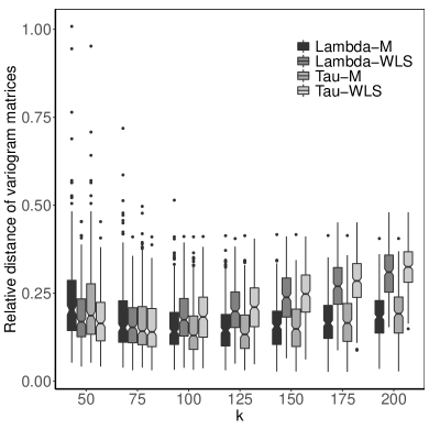
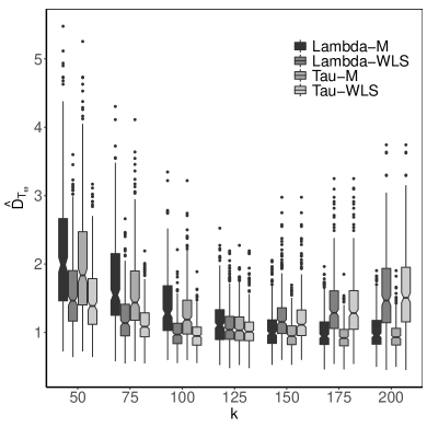
Figure 2: Boxplots of $\frac{\|\hat{\bm{\Gamma}}_{M}-\bm{\Gamma}\|_{F}}{\|\bm{\Gamma}\|_{F}}$ (left) and $\hat{D}_{\mathcal{T}_{\omega}}$ in (4.8) (right) for $10$-dimensional Hüsler–Reiss distribution with variogram matrix $\bm{\Gamma}_{3}$ based on $\hat{\mathcal{T}}_{\lambda}^{\star}$ (Lambda) and $\hat{\mathcal{T}}_{\tau}^{\star}$ (Tau), where bivariate stable tail dependence functions are fitted based on M-estimator (M) and weighted least squares estimator (WLS) at $k=50,75,\ldots,200$ ($300$ samples of size $n=1000$)

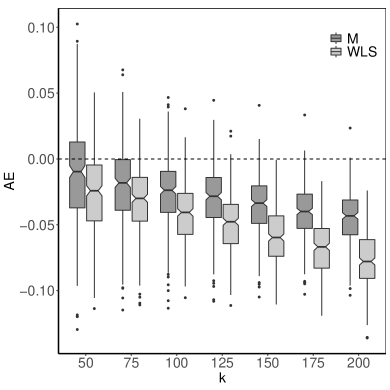
Figure 3: Boxplot of the approximation errors of the rare event probability in (5.3) based on $\hat{\mathcal{T}}_{\tau}^{\star}$ for $10$-dimensional Hüsler–Reiss distribution with variogram matrix $\bm{\Gamma}_{3}$, where bivariate stable tail dependence functions are fitted using the M-estimator (M) and the weighted least squares estimator (WLS) at $k=50,75,\ldots,200$, the levels $u_{1},u_{2},u_{3}$ are taken as the $0.999$ empirical marginal quantiles and $u_{j}=\infty$ for $j=4,\ldots,d$ ($300$ samples of size $n=1000$)

For samples generated from the $10$-dimensional Hüsler–Reiss distribution with variogram matrix $\bm{\Gamma}_{4}$ which is not necessarily tree-structured, the simulation results have similar patterns as those in the first case but with larger errors. The variogram matrix $\bm{\Gamma}_{4}$ and boxplots can be found in Table 4 and Fig. 7–8 in Appendix A.2.

5.2 Asymmetric logistic distribution

In reality, we do not know the true distribution $G$. The bivariate distribution family we use to model adjacent pairs may be different from the true one. To see the estimation error in this scenario, we generate samples from the $5$-dimensional asymmetric logistic distribution in Example 3.4 (a special max-linear model) with randomly generated parameter $\bm{\Psi}_{3}=(0.763,0.835,0.602,0.747,0.859)$. Still, we model the adjacent pairs on the constructed Markov tree by bivariate Hüsler–Reiss distributions.

According to Fig. 4, the two types of edges weights, $\lambda$ and $\tau$, still exhibit a similar performance. Larger $k$ leads to a higher accuracy for both estimators in terms of $\hat{D}_{\mathcal{T}_{\omega}}$, while the weighted least squares estimator behaves better than the M-estimator for the chosen $k$, as can also be seen from the approximation error on the right-hand panel in the figure. However, compared with the experiments for the Hüsler–Reiss distribution above, the approximation errors are much larger.

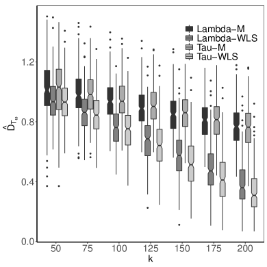
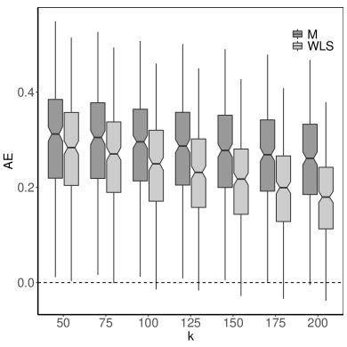
Figure 4: Boxplots of $\hat{D}_{\mathcal{T}_{\omega}}$ (left) in (4.8) based on $\hat{\mathcal{T}}_{\lambda}^{\star}$ (Lambda) and $\hat{\mathcal{T}}_{\tau}^{\star}$ (Tau) and the approximation errors (right) of the rare event probability in (5.3) based on $\hat{\mathcal{T}}_{\tau}^{\star}$ for $5$-dimensional asymmetric logistic distribution with parameter vector $\bm{\Psi}_{3}$ in Section 5.2, where bivariate Hüsler–Reiss stable tail dependence functions are fitted with M-estimator (M) and weighted least squares estimator (WLS) at $k=50,75,\ldots,200$ ($300$ samples of size $n=1000$)

6 Application

In this section we consider the average daily discharges recorded at $31$ gauging stations in the upper Danube basin covering parts of Germany, Austria and Switzerland. The topographic map can be found in Figure 1 of Asadi et al., (2015) and the data are available in the supplementary materials of that paper. The series at individual stations have lengths from $54$ to $113$ years, with $51$ years of data for all stations from $1960$ to $2010$. The average daily discharges were measured in $m^{3}/s$, ranging from $20$ to $1400$. Following Asadi et al., (2015) and Engelke & Hitz, (2020), we only consider the daily discharges in the summer months (June, July and August) to get rid of the seasonality. The information for summer discharges at each station is given in Table 5 of Appendix A.2.

For $i=1,\ldots,n$, denote the daily mean discharges at the station $j$ on day $i$ by $\xi_{i,j}$ and assume the distribution function of $\bm{\xi}^{i}=(\xi_{i,1},\ldots,\xi_{i,d})$ belongs to the domain of attraction of a multivariate extreme value distribution function. We are concerned about the probability that there will be a flood above a certain (high) threshold for at least one site within the considered stations, precisely, the probability in (1.1). In view of (5.2), the modelling can be split into two parts: fitting the marginal distributions and estimating the simple tree-based multivariate extreme distribution function $G_{M}$.

Extreme discharges often occur in clusters. To remove the clusters and create a sequence of independent and identically distributed variables, we follow the procedure in Asadi et al., (2015) for each of the $51$ summer periods. It ranks the data within each series and starts from the day with the highest rank of the period across all series (only one series when extracting univariate events) and takes a window of $9$ days. An event is formed by taking the largest observation within this window. Then the data in this window are deleted and the process is repeated to form a new event. All events are found when no window of $9$ consecutive days remains.

6.1 Marginal fitting

Under the assumption that the distribution of $\bm{\xi}^{i}$ belongs to the domain of attraction of a multivariate extreme value distribution, the marginal distributions are also attracted by univariate extreme value distributions. In line with asymptotic theory, we model high-threshold excesses by the generalized Pareto distribution to obtain the margins $F_{j}$ for $j=1,\ldots,d$. Since the extremal behavior from any available earlier data does not change relative to the $51$ common years, see Asadi et al., (2015), all the available data for each station are used to do the marginal fitting.

For $j=1,\ldots,d$ and $0<p<1$, let $q_{j,p}$ be the empirical $p$-quantile of $\xi_{i,j}$ and put $\mathcal{I}_{j}=\{i\in\{1,\ldots,n\}:\xi_{i,j}>q_{j,p}\}$. For each station $j$, let $\hat{\sigma}_{j}>0$ and $\hat{\vartheta}_{j}\in\mathbb{R}$ be the maximum likelihood estimates of the scale and shape parameters of the generalized Pareto distribution fitted to the excesses $\xi_{i,j}-q_{j,p}$ for $i\in\mathcal{I}_{j}$. Let $N_{j}$ and $n_{j}$ denote the sample size at station $j$ and the number of elements in $\mathcal{I}_{j}$, respectively. Then the tail distribution function $1-F_{j}$ is estimated by

$$1-\hat{F}_{j}(x)=\frac{n_{j}}{N_{j}}\left\{1-\operatorname{GPD}(x-q_{j,p};\hat{\sigma}_{j},\hat{\vartheta}_{j})\right\},$$ (6.1)

where $\operatorname{GPD}(\,\cdot\,;\sigma,\vartheta)$ denotes the cumulative distribution function of the generalized Pareto distribution with scale parameter $\sigma>0$ and shape parameter $\vartheta\in\mathbb{R}$.

In pursuit of a good fit, an appropriate threshold $q_{j,p}$ has to be found. By inspection of the mean residual life plot, it was decided to set the threshold for margin $j$ equal to $q_{j,p}$ for $p=0.9$. The number of declustered excesses used for the estimation at each station as well as the corresponding thresholds $q_{j,p}$ and maximum likelihood estimates of $\hat{\sigma}_{j}$ and $\hat{\vartheta}_{j}$ of fitted generalized Pareto distribution for $j=1,\ldots,31$ are given in Tables 6 and 7 of Appendix A.3 respectively.

6.2 Estimation of the dependence structure

In this subsection, we approximate the dependence structure between extremes of the $31$ gauging stations by a multivariate extreme value distributions $G_{M}$ related to a Markov tree. After declustering, there are $N=428$ independent observations from the $51$ years of data for all stations. The tree structure corresponding to the physical flow connections at these stations is presented in Fig. 9, while the tree structures $\hat{\mathcal{T}}_{\lambda}^{\star}$ and $\hat{\mathcal{T}}_{\tau}^{\star}$ (4.3) are given in Fig. 10 of Appendix A.3. We construct the extreme value distribution $G_{M}$ by fitting the Hüsler–Reiss distribution to all pairs of connected variables and estimate their parameters by the moments estimator, the M-estimator and the weighted least squares estimator with $k=65$. The estimated GPD-based marginal probability in (6.1) and the probability $\operatorname{\mathbb{P}}\left(\xi_{4}>u_{4}~{}\text{or}~{}\xi_{7}>u_{7}~{}\text{or}~{}\xi_{13}>u_{13}\right)$ of flooding at one or more stations $4$, $7$ and $13$, which are connected differently on the maximum dependence trees $\hat{\mathcal{T}}_{\lambda}^{\star}$ and $\hat{\mathcal{T}}_{\tau}^{\star}$ (Fig. 10 of Appendix A.3), are given in Tables 2 and 3 respectively, where $u_{j}$ for $j=4,7,13$ are taken as the $0.95$, $0.99$, $0.995$ and $0.999$ empirical quantiles of the $51$-year samples. Compared with the empirical probabilities, the tree-based model yields higher estimates of the flooding probabilities. As shown in Table 2, this may be partly due to the difference between the non-parametric and GPD-based estimates of the marginal probabilities $F_{j}(u_{j})$ for $j=4,7,13$.

Table 2: GPD-based estimates $1-\hat{F}_{j}(u_{j})$ of marginal tail probability in (6.1) with $u_{j}$ taken as the $0.95$, $0.99$, $0.995$ and $0.999$ empirical quantiles of the $51$-year samples for $j=4,7,13$

$u_{j}$	$q_{j,0.95}$	$q_{j,0.99}$	$q_{j,0.995}$	$q_{j,0.999}$
$1-\hat{F}_{4}$	$6.52\%$	$1.87\%$	$0.99\%$	$0.22\%$
$1-\hat{F}_{7}$	$6.66\%$	$1.69\%$	$1.03\%$	$0.15\%$
$1-\hat{F}_{13}$	$7.02\%$	$1.90\%$	$1.18\%$	$0.33\%$

Table 3: Empirical and model-based estimates of the flooding probability (1.1) over the $0.95$, $0.99$, $0.995$ and $0.999$ empirical quantiles of the $51$-year samples at stations $4$, $7$ and $13$ in the upper Danube basin, where bivariate Hüsler–Reiss stable tail dependence functions of connected pairs on maximum dependence tree $\hat{\mathcal{T}}_{\lambda}^{\star}$ and $\hat{\mathcal{T}}_{\tau}^{\star}$ are fitted with moments estimator (MM), M-estimator (M) and weighted least squares estimator (WLS) at $k=65$

	$u_{j}$	$q_{j,0.95}$	$q_{j,0.99}$	$q_{j,0.995}$	$q_{j,0.999}$
Empirical		$8.44\%$	$1.88\%$	$1.02\%$	$0.21\%$
$\hat{\mathcal{T}}_{\lambda}^{\star}$	MM	$9.71\%$	$2.65\%$	$1.58\%$	$0.38\%$
	M	$9.72\%$	$2.65\%$	$1.58\%$	$0.38\%$
	WLS	$9.62\%$	$2.62\%$	$1.56\%$	$0.37\%$
$\hat{\mathcal{T}}_{\tau}^{\star}$	MM	$9.54\%$	$2.61\%$	$1.55\%$	$0.37\%$
	M	$9.55\%$	$2.61\%$	$1.55\%$	$0.37\%$
	WLS	$9.26\%$	$2.53\%$	$1.50\%$	$0.37\%$

Address

Shuang Hu,

School of Mathematics and Statistics, Southwest University, 400715 Chongqing, China.

LIDAM/ISBA, Université catholique de Louvain, B1348 Louvain-la-Neuve, Belgium.

E-mail address: hs1995@email.swu.edu.cn

Appendix A Appendix

A.1 Proofs

Proof of Proposition 2.3.

By assumption, there exists a regularly varying Markov tree $\bm{Y}$ satisfying Condition 2.1 and (2.7) such that $\bm{Y}\in D(G)$, where $G$ is a simple multivariate extremes value distribution transformed from $H$. Moreover, $G$ and $H$ have the same stable tail dependence functions. Thus it is sufficient to derive the result in terms of $G$. Let $v_{1},\ldots,v_{d}$ be an arbitrary permutation of $1,\ldots,d$. Since $\bm{Y}$ satisfies Condition 2.1, it follows from (2.7) and Theorem 2 in Segers, (2020) that

$$n\operatorname{\mathbb{P}}\left(\bigcup_{v=1}^{d}\{Y_{v}>ny_{v}\}\right)$$

$$=n\sum_{i=1}^{d-1}\operatorname{\mathbb{P}}(Y_{v_{i}}>ny_{v_{i}},Y_{v_{j}}\leq ny_{v_{j}},j=i+1,\ldots,d)+n\operatorname{\mathbb{P}}(Y_{v_{d}}>ny_{v_{d}})$$

$$=\sum_{i=1}^{d-1}n\operatorname{\mathbb{P}}(Y_{v_{i}}>ny_{v_{i}})\operatorname{\mathbb{P}}(Y_{v_{j}}\leq ny_{v_{j}},j=i+1,\ldots,d\mid Y_{v_{i}}>ny_{v_{i}})+n\operatorname{\mathbb{P}}(Y_{v_{d}}>ny_{v_{d}})$$

$$\to\sum_{i=1}^{d}y_{v_{i}}^{-1}\operatorname{\mathbb{P}}\left(W\Theta_{v_{i},v_{j}}\leq y_{v_{j}}/y_{v_{i}},j=i+1,\ldots,d\right)$$ (A.1)

as $n\to\infty$, where the probability in the sum (A.1) is interpreted as $1$ for $i=d$. Recall that $W$ is unit-Pareto distributed and is independent of $\bm{\Theta}_{v_{i}}$. By the fact that $1/W$ is uniformly distributed on $[0,1]$, we have

$$y_{v_{i}}^{-1}\operatorname{\mathbb{P}}\left(W\Theta_{v_{i},v_{j}}\leq y_{v_{j}}/y_{v_{i}},j=i+1,\ldots,d\right)$$

$$=y_{v_{i}}^{-1}\int_{0}^{1}\operatorname{\mathbb{P}}\left\{\Theta_{v_{i},v_{j}}\leq(y_{v_{j}}u)/y_{v_{i}},j=i+1,\ldots,d\right\}\operatorname{d}{u}$$

$$=y_{v_{i}}^{-1}\int_{0}^{1}\operatorname{\mathbb{P}}\left\{\max_{j=i+1,\ldots,d}\left(y_{v_{j}}^{-1}\Theta_{v_{i},v_{j}}\right)\leq y_{v_{i}}^{-1}u\right\}\operatorname{d}{u}$$

$$=\int_{0}^{1/y_{v_{i}}}\operatorname{\mathbb{P}}\left\{\max_{j=i+1,\ldots,d}\left(y_{v_{j}}^{-1}\Theta_{v_{i},v_{j}}\right)\leq u\right\}\operatorname{d}{u}$$

$$=\int_{0}^{\infty}\operatorname{\mathbb{P}}\left\{\max_{j=i+1,\ldots,d}\left(y_{v_{j}}^{-1}\Theta_{v_{i},v_{j}}\right)\leq u\leq y_{v_{i}}^{-1}\Theta_{v_{i},v_{i}}\right\}\operatorname{d}{u}$$

$$=\operatorname{\mathbb{E}}\left\{\max_{j=i,\ldots,d}\left(y_{v_{j}}^{-1}\Theta_{v_{i},v_{j}}\right)-\max_{j=i+1,\ldots,d}\left(y_{v_{j}}^{-1}\Theta_{v_{i},v_{j}}\right)\right\},$$ (A.2)

where the last step follows from $\int_{0}^{\infty}\operatorname{\mathbb{P}}(A\leq u\leq B)\operatorname{d}u=\operatorname{\mathbb{E}}[\int_{0}^{\infty}\operatorname{\mathbbm{1}}(A\leq u\leq B)\operatorname{d}{u}]=\operatorname{\mathbb{E}}[\max(A,B)-A]$ for non-negative random variables $A$ and $B$. By (2.1) with $a_{n,v}=n$ and $b_{n,v}=0$, (A.1)–(A.1) and (2.2), we have

$$\ell(\bm{y}) =-\log G(1/y_{1},\ldots,1/y_{d})=\lim_{n\to\infty}n\operatorname{\mathbb{P}}\left(\bigcup_{v=1}^{d}\{Y_{v}>ny_{v}\}\right)$$

$$=\sum_{i=1}^{d}\operatorname{\mathbb{E}}\left\{\max_{j=i,\ldots,d}\left(y_{v_{j}}\Theta_{v_{i},v_{j}}\right)-\max_{j=i+1,\ldots,d}\left(y_{v_{j}}\Theta_{v_{i},v_{j}}\right)\right\},$$ (A.3)

where the maximum over the empty set is defined as zero. The identity $\Theta_{v_{i},v_{j}}=\prod_{e\in[{v_{i}}\rightsquigarrow{v_{j}}]}M_{e}$ yields the desired expression of $\ell$, which is totally determined by the distributions of the increments $M_{e}$ with $e\in E$.

Assume $\operatorname{\mathbb{E}}(M_{ab})=1$ for all $(a,b)\in E$. Then $\operatorname{\mathbb{E}}(\Theta_{u,v})=\prod_{(a,b)\in[{u}\rightsquigarrow{v}]}\operatorname{\mathbb{E}}(M_{ab})=1$ for $u,v\in V$ by the independence of $M_{e}$ for $e\in E$. Thus it follows from Corollary 3 in Segers, (2020) that the root-change formula

$$\operatorname{\mathbb{E}}\left\{g(\bm{\Theta}_{u})\right\}=\frac{\operatorname{\mathbb{E}}\left\{g\left(\bm{\Theta}_{v}/\Theta_{v,u}\right)\Theta_{v,u}\right\}}{\operatorname{\mathbb{E}}(\Theta_{v,u})}$$

holds for any Borel measurable function $g:[0,\infty)^{d}\setminus\{\bm{0}\}\rightarrow[0,\infty]$, where $\bm{0}$ denotes the $d$-dimensional vector whose components are zero. For fixed $\bm{y}=(y_{v},v\in V)$, taking $g_{i}(\bm{x})=\max_{j=i,\ldots,d}\left(y_{v_{j}}x_{v_{j}}\right)$ for $i=2,\ldots,d$ and using the root-change formula we have

$$\operatorname{\mathbb{E}}\left\{\max_{j=i,\ldots,d}\left(y_{v_{j}}\Theta_{v_{i},v_{j}}\right)\right\} =\operatorname{\mathbb{E}}\left[\max_{j=i,\ldots,d}\left\{y_{v_{j}}\Theta_{v_{i},v_{j}}\operatorname{\mathbbm{1}}(\Theta_{v_{i},v_{i-1}}>0)\right\}\right]$$

$$=\operatorname{\mathbb{E}}\left[\Theta_{v_{i},v_{i-1}}\max_{j=i,\ldots,d}\left\{\left(y_{v_{j}}\Theta_{v_{i},v_{j}}\right)/\Theta_{v_{i},v_{i-1}}\right\}\right]$$

$$=\operatorname{\mathbb{E}}\left\{\max_{j=i,\ldots,d}\left(y_{v_{j}}\Theta_{v_{i-1},v_{j}}\right)\right\}\operatorname{\mathbb{E}}\left(\Theta_{v_{i},v_{i-1}}\right)$$

$$=\operatorname{\mathbb{E}}\left\{\max_{j=i,\ldots,d}\left(\ y_{v_{j}}\Theta_{v_{i-1},v_{j}}\right)\right\},$$

where the first step holds since $\operatorname{\mathbb{E}}(\Theta_{v_{i-1},v_{i}})=1$ implies $\operatorname{\mathbb{P}}(\Theta_{v_{i},v_{i-1}}>0)=1$ by Corollary 3 in Segers, (2020). Consequently, in view of (A.1) and the above equality we obtain

$$\ell(\bm{y}) =\sum_{i=1}^{d}\operatorname{\mathbb{E}}\left\{\max_{j=i,\ldots,d}\left(y_{v_{j}}\Theta_{v_{i},v_{j}}\right)\right\}-\sum_{i=2}^{d}\operatorname{\mathbb{E}}\left\{\max_{j=i,\ldots,d}\left(y_{v_{j}}\Theta_{v_{i-1},v_{j}}\right)\right\}$$

$$=\operatorname{\mathbb{E}}\left\{\max_{j=1,\ldots,d}\left(y_{v_{j}}\Theta_{v_{1},v_{j}}\right)\right\}.$$

The final identity holds because $v_{1},\ldots,v_{d}$ was an arbitrary permutation of $1,\ldots,d$. ∎

Proof of Proposition 2.4.

For $y_{a},y_{b}\geq 0$, setting $d=2$ in (2.9) and using the relation $\max(x,y)=x+y-\min(x,y)$ yields

$$\ell_{ab}(y_{a},y_{b}) =\operatorname{\mathbb{E}}\left\{\max\left(y_{a},y_{b}\prod_{e\in[{a}\rightsquigarrow{b}]}M_{e}\right)-y_{b}\prod_{e\in[{a}\rightsquigarrow{b}]}M_{e}\right\}+y_{b}$$

$$=y_{a}+y_{b}-\operatorname{\mathbb{E}}\left\{\min\left(y_{a},y_{b}\prod_{e\in[{a}\rightsquigarrow{b}]}M_{e}\right)\right\}.$$

The desired result for $\lambda_{ab}$ follows since $\lambda_{ab}=2-\ell_{ab}(1,1)$. The proof is complete. ∎

Proof of Proposition 2.5.

Let $\bm{Y}=(Y_{v},v\in V)$ be the Markov tree on $\mathcal{T}$ associated to $H$ in Definition 2.2. For each pair $(a,b)\in E$, the tail dependence coefficient of $(Y_{a},Y_{b})$ equals the one of $(X_{a},X_{b})$. Thus it is sufficient to derive the result in terms of $\bm{Y}$.

For $\delta>0$, note that

$$n\operatorname{\mathbb{P}}(Y_{a}>n\delta,Y_{b}>n)\leq n\operatorname{\mathbb{P}}(Y_{b}>n)\to 1$$ (A.4)

as $n\to\infty$ by (2.7). From the equality

$$\int_{0}^{x}\operatorname{\mathbb{P}}(X>u)\operatorname{d}u=\operatorname{\mathbb{E}}\{\min(X,x)\}$$

for a non-negative random variable $X$ and for $x>0$, we find by (2.7), (2.8) and the fact that $1/W$ is uniformly distributed on $[0,1]$ that

$$n\operatorname{\mathbb{P}}(Y_{a}>n\delta,Y_{b}>n) =n\operatorname{\mathbb{P}}(Y_{a}>n\delta)\cdot\operatorname{\mathbb{P}}(Y_{b}>n\mid Y_{a}>n\delta)$$

$$\to\delta^{-1}\operatorname{\mathbb{P}}(WM_{ab}>1/\delta)=\delta^{-1}\operatorname{\mathbb{P}}(\delta M_{ab}>1/W)$$

$$=\delta^{-1}\operatorname{\mathbb{E}}\{\min(\delta M_{ab},1)\}=\operatorname{\mathbb{E}}\{\min(M_{ab},1/\delta)\}$$

as $n\to\infty$. Combining the above display with (A.4) and letting $\delta\to 0$ we obtain

$$\operatorname{\mathbb{E}}(M_{ab})\leq 1,\qquad(a,b)\in E.$$ (A.5)

The concavity of the function $y\mapsto\min(1,xy)$ implies that

$$\min(1,xy)\leq\min(1,x)-\left(1-y\right)x\operatorname{\mathbbm{1}}(x<1),\qquad(x,y)\in[0,\infty)^{2},$$ (A.6)

as can be confirmed by a case-by-case analysis. Let $u$ be a node on the path from $a$ to $b$ and write $A=\prod_{e\in[{a}\rightsquigarrow{u}]}M_{e}$ and $B=\prod_{e\in[{u}\rightsquigarrow{b}]}M_{e}$. We have $\operatorname{\mathbb{E}}[B]\leq 1$ by (A.5) and the independence of the increments $M_{e}$ for $e\in E$. Using Proposition 2.4, we have, since $A$ and $B$ are independent and non-negative,

$$\lambda_{ab}=\operatorname{\mathbb{E}}\{\min(1,AB)\} \leq\operatorname{\mathbb{E}}\{\min(1,A)\}-\left\{1-\operatorname{\mathbb{E}}(B)\right\}\operatorname{\mathbb{E}}\{A\operatorname{\mathbbm{1}}(A<1)\}$$ (A.7)

$$\leq\operatorname{\mathbb{E}}\{\min(1,A)\}=\lambda_{au}.$$

Interchanging the roles of $A$ and $B$ yields $\lambda_{ab}\leq\lambda_{ub}$. The inequality (A.6) is strict whenever $x>1>xy$ or $x<1<xy$. If $\operatorname{\mathbb{P}}(1-\varepsilon<M_{e}<1)>0$ and $\operatorname{\mathbb{P}}(1<M_{e}<1+\varepsilon)>0$ for every $e\in E$ and every $\varepsilon>0$, then also $\operatorname{\mathbb{P}}(A>1>AB)>0$ and $\operatorname{\mathbb{P}}(A<1<AB)>0$. But then $\min(1,AB)<\min(1,A)-\left(1-B\right)A\operatorname{\mathbbm{1}}(A<1)$ with positive probability, yielding a strict inequality in (A.7).

As for the lower bound, the inequality $\min(1,s)\min(1,t)\leq\min(1,st)$ for non-negative reals $s$ and $t$ and the independence of $M_{e}$, $e\in E$, yields, with $A$ and $B$ as above,

$$\lambda_{ab}=\operatorname{\mathbb{E}}\{\min(1,AB)\}\geq\operatorname{\mathbb{E}}\{\min(1,A)\min(1,B)\}=\operatorname{\mathbb{E}}\{\min(1,A)\}\operatorname{\mathbb{E}}\{\min(1,B)\}=\lambda_{au}\lambda_{ub},$$

as required. The proof is complete. ∎

Derivation of Eq. (3.4).

For $x_{v}\in\mathbb{R}$ such that $v\in V$, we have, by the maximum-minimums identity

$$\max_{v\in V}x_{v}=\sum_{\emptyset\neq U\subseteq V}(-1)^{|U|+1}\min_{v\in U}x_{v}.$$

Recall that $V_{i}=\{i,\ldots,d\}$ and $e=(e_{p},e_{s})$ for $e\in E$. Without loss of generality, let $v_{i}=i$ for the permutation $v_{1},\ldots,v_{d}$ of $1,\ldots,d$ in Corollary 3.2 and (2.9). Then, in view of the distribution of $M_{e}$ for $e\in E$ given in Eq. (3.14) and by applying the above display, we have from Corollary 3.2 that

$$\ell^{M}(\bm{y})= \sum_{i=1}^{d}\operatorname{\mathbb{E}}\left\{\max_{j=i,\ldots,d}\left(y_{j}\prod_{e\in[{i}\rightsquigarrow{j}]}M_{e}\right)\right\}-\sum_{i=2}^{d}\operatorname{\mathbb{E}}\left\{\max_{j=i,\ldots,d}\left(y_{j}\prod_{e\in[{(i-1)}\rightsquigarrow{j}]}M_{e}\right)\right\}$$

$$= \sum_{i=1}^{d}\sum_{\emptyset\neq U\subseteq V_{i}}(-1)^{|U|+1}\operatorname{\mathbb{E}}\left\{\min_{j\in U}\left(y_{j}\prod_{e\in[{i}\rightsquigarrow{j}]}M_{e}\right)\right\}$$

$$-\sum_{i=2}^{d}\sum_{\emptyset\neq U\subseteq V_{i}}(-1)^{|U|+1}\operatorname{\mathbb{E}}\left\{\min_{j\in U}\left(y_{j}\prod_{e\in[{(i-1)}\rightsquigarrow{j}]}M_{e}\right)\right\}$$

$$= \sum_{i=1}^{d}\psi_{i}^{-1}\sum_{\emptyset\neq U\subseteq V_{i}}(-1)^{|U|+1}\left(\prod_{e\in\bigcup_{j\in U}[{i}\rightsquigarrow{j}]}\psi_{e_{p}}\right)\left\{\min_{j\in U}\left(y_{j}\psi_{j}\right)\right\}$$

$$-\sum_{i=2}^{d}\psi_{i-1}^{-1}\sum_{\emptyset\neq U\subseteq V_{i}}(-1)^{|U|+1}\left(\prod_{e\in\bigcup_{j\in U}[{(i-1)}\rightsquigarrow{j}]}\psi_{e_{p}}\right)\left\{\min_{j\in U}\left(y_{j}\psi_{j}\right)\right\}.\qed$$

Proof of Proposition 4.1.

Let $\mathcal{T}^{\prime}=(V,E^{\prime})$ be any tree with the same node set $V$ as the true tree $\mathcal{T}=(V,E)$. As in the proof of Proposition 5 in Engelke & Volgushev, (2020), an application of Hall’s marriage theorem (Hall,, 1935) yields a bijection $f:E\to E^{\prime}$ with the property that every edge $(u,v)\in E$ is mapped to an edge $f((u,v))=(u^{\prime},v^{\prime})\in E^{\prime}$ such that $(u,v)$ belongs to the path $[{u^{\prime}}\rightsquigarrow{v^{\prime}}]$ in $\mathcal{T}$. By Proposition 2.5, $\lambda_{uv}\geq\lambda_{f(u,v)}$ and thus

$$S_{\mathcal{T}_{\lambda}}=\sum_{(u,v)\in E}\lambda_{uv}\geq\sum_{(u,v)\in E}\lambda_{f(u,v)}=\sum_{(u^{\prime},v^{\prime})\in E^{\prime}}\lambda_{u^{\prime}v^{\prime}}=S_{\mathcal{T}_{\lambda}^{\prime}}.$$

It follows that $\mathcal{T}$ belongs to the collection $\bm{T}_{\lambda}^{\star}$ of maximum tail dependence trees.

Suppose in addition that $\lambda_{ab}<\min(\lambda_{au},\lambda_{ub})$ for any triple of distinct nodes $a,u,b$ such that $u$ lies on the path between $a$ and $b$. If $\mathcal{T}^{\prime}=(V,E^{\prime})$ is different from $\mathcal{T}$, then there is at least one edge $(u,v)\in E$ such that $f((u,v))=(u^{\prime},v^{\prime})$ is different from $(u,v)$. By the additional condition, we then have $\lambda_{uv}>\lambda_{u^{\prime}v^{\prime}}$. The inequality in the above display is thus strict, implying that $\mathcal{T}$ is the unique maximizer of the sum of edge weights. ∎

Proof of Proposition 4.2.

Let $\mathcal{T}^{\star}=(V,E^{\star})$ be an arbitrary tree in $\bm{T}_{\lambda}^{\star}$. We show that for any tree $\mathcal{T}^{\prime}=(V,E^{\prime})$ not in $\bm{T}_{\lambda}^{\star}$, we have

$$\operatorname{\mathbb{P}}\left(\hat{S}_{\mathcal{T}_{\lambda}^{\prime}}<\hat{S}_{\mathcal{T}_{\lambda}^{\star}}\right)\to 1,\quad n\to\infty.$$ (A.8)

By definition of $\hat{\bm{T}}_{\lambda}^{\star}$, this implies

$$\operatorname{\mathbb{P}}\left(\mathcal{T}^{\prime}\in\hat{\bm{T}}_{\lambda}^{\star}\right)\to 0,\quad n\to\infty.$$

As this is true for any $\mathcal{T}^{\prime}$ not in $\bm{T}_{\lambda}^{\star}$, we can then conclude that $\operatorname{\mathbb{P}}\left(\hat{\bm{T}}_{\lambda}^{\star}\subseteq\bm{T}_{\lambda}^{\star}\right)\to 1$ as $n\to\infty$.

To show (A.8), note that, by definition of $\bm{T}_{\lambda}^{\star}$, we have

$$S_{\mathcal{T}_{\lambda}^{\prime}}<S_{\mathcal{T}_{\lambda}^{\star}}.$$

The consistency of the empirical tail dependence coefficients $\hat{\lambda}_{e}$ for $e\in E$ (Drees & Huang,, 1998; Schmidt & Stadtmüller,, 2006) implies

$$\hat{S}_{\mathcal{T}_{\lambda}^{\prime}}-\hat{S}_{\mathcal{T}_{\lambda}^{\star}}=\sum_{e\in E^{\prime}}\hat{\lambda}_{e}-\sum_{e\in E^{\star}}\hat{\lambda}_{e}=\sum_{e\in E^{\prime}}\lambda_{e}-\sum_{e\in E^{\star}}\lambda_{e}+o_{p}(1)=S_{\mathcal{T}_{\lambda}^{\prime}}-S_{\mathcal{T}_{\lambda}^{\star}}+o_{p}(1),\quad n\to\infty,$$

yielding the convergence in (A.8), as required.

If $\bm{T}_{\lambda}^{\star}$ is a singleton, say $\{\mathcal{T}_{\lambda}^{\star}\}$, then the relation $\hat{\bm{T}}_{\lambda}^{\star}\subseteq\bm{T}_{\lambda}^{\star}$ implies that $\hat{\bm{T}}_{\lambda}^{\star}$ (which is non-empty since it is the set of maximizers over a finite domain) is a singleton too and that its only element, say $\hat{\mathcal{T}}_{\lambda}^{\star}$, is equal to $\mathcal{T}_{\lambda}^{\star}$. ∎

Proof of Theorem 4.4.

By Theorem 5.1 in Bücher et al., (2014), we have weak convergence of $\alpha_{n}=\sqrt{k}(\hat{\ell}_{n,k}-\ell)$ in the so-called hypi-topology on the set of bounded functions on $[0,1]^{d}$ to a process which, thanks to the condition on the $\mu_{r}$-almost everywhere continuity of $\dot{\ell}_{j}$, is $\mu_{r}$-almost everywhere equal to $\alpha$ in (4.4). By Corollary 3.3 in the same article and again by the assumption on $\dot{\ell}_{j}$, we obtain the weak convergence of $\alpha_{n}$ to $\alpha$ in $L^{2}(\mu_{r})$; indeed, with probability one, the process $\alpha$ is continuous $\mu_{r}$-almost everywhere, thanks to the assumption on $\dot{\ell}_{j}$ and the fact that $W(\bm{0})=0$. The linear functional $L^{2}(\mu_{r})\to\mathbb{R}:f\mapsto\int f\psi_{r}\,\operatorname{d}\mu_{r}$ for $r\in\{1,\ldots,q\}$ being continuous, an application of the continuous mapping theorem yields the result. The limit in (4.5) is a linear transformation of a Gaussian process and therefore Gaussian as well. The formula for the covariance matrix follows by Fubini’s theorem.

An alternative proof is to proceed by a Skorohod construction as in the proof of Proposition 7.3 in Einmahl et al., (2012). The term involving the partial derivatives $\dot{\ell}_{j}$ is handled via the dominated convergence theorem: the pointwise convergence for $\mu_{r}$-almost every $\bm{x}\in[0,1]^{d}$ holds true thanks to the condition on the partial derivatives $\dot{\ell}_{j}$. ∎

Proof of Corollary 4.7.

For $e=(a,b)\in E$, the map

$$T_{e}:[0,1]^{2}\to[0,1]^{d}:(x_{a},x_{b})\mapsto x_{a}\bm{e}_{a}+x_{b}\bm{e}_{b}$$

pushes the measure $\nu_{e}$ on $[0,1]^{2}$ forward to the measure $\mu_{e}=T_{e}\#\nu_{e}$ on $[0,1]^{d}$ given by

$$\mu_{e}(A)=\nu_{e}\left(\left\{(x_{a},x_{b})\in[0,1]^{2}:x_{a}\bm{e}_{a}+x_{b}\bm{e}_{b}\in A\right\}\right)$$

for Borel sets $A\subseteq[0,1]^{d}$. The support of $\mu_{e}$ is contained in $\{\bm{x}\in[0,1]^{d}:x_{j}=0~{}\text{if}~{}j\neq a~{}\text{and}~{}j\neq b\}$. By the change-of-variables formula, integrals with respect to $\mu_{e}$ and $\nu_{e}$ are related through $\int_{[0,1]^{d}}f(\bm{x})\,\mu_{e}(\operatorname{d}\bm{x})=\int_{[0,1]^{2}}f(T_{e}(x_{a},x_{b}))\,\nu_{e}(\operatorname{d}(x_{a},x_{b}))$.

Put $\alpha_{n}=\sqrt{k}(\hat{\ell}_{n,k}-\ell)$. By Slutsky’s lemma, the $o_{p}(\bm{1})$ term in Assumption 4.6 does not matter for the convergence in distribution. Since $\hat{\ell}_{n,k,e}(x_{a},x_{b})=\hat{\ell}_{n,k}(T_{e}(x_{a},x_{b}))$ and similarly for $\ell_{e}$ and $\ell$, the main term on the right-hand side of (4.6) can be written as

$$\int_{[0,1]^{d}}\alpha_{n}(\bm{x})\,\bm{\psi}_{e}(x_{a},x_{b})\,\mu_{e}(\operatorname{d}\bm{x}).$$

This is a random vector of dimension $p_{e}$, each component of which has the same form as the entries of the random vector on the left-hand side of (4.5). Indeed, the measure $\mu_{r}$ in (4.5) is equal to the measure $\mu_{e}$ here, while the function $\psi_{r}$ in (4.5) is the equal to the function $\bm{x}\mapsto\psi_{e,j}(x_{a},x_{b})$ here, where $\psi_{e,j}$ is one of the $p_{e}$ component functions of $\bm{\psi}_{e}$. The conclusion now follows from Theorem 4.4; Assumption 4.6(ii) ensures that the smoothness condition in Theorem 4.4 is fulfilled. ∎

A.2 Additional material and results for simulation study in Section 5

In this subsection, we list some additional material for the simulation study: Prim’s algorithm in Algorithm 1; the simulation and fitting procedure for Hüsler–Reiss distributions in Algorithm 2; the variogram matrices $\bm{\Gamma}_{3}$ and $\bm{\Gamma}_{4}$ in Table 4; the tree structure in Fig. 5; the simulation results for the proportion of misidentified trees in $300$ replications for the $10$-dimensional Hüsler–Reiss distribution in Fig. 6; and the boxplots of $\frac{\|\hat{\bm{\Gamma}}_{M}-\bm{\Gamma}\|_{F}}{\|\bm{\Gamma}\|_{F}}$, $\hat{D}_{\mathcal{T}_{\omega}}$ and the estimation error of rare event probability in Fig. 7–8.

1. Choose a starting point $v\in V$. Define the node set and edge set of the maximum dependence tree as $V^{\prime}=\{v\}$ and $E^{\prime}=\emptyset$.

2. While $V^{\prime}\neq V$, choose an edge $e=(a,b)$ with maximal weight $\hat{\omega}_{ab}$ such that $a\in V^{\prime}$ and $b\notin V^{\prime}$.

3. Set $V^{\prime}=V^{\prime}\cup\{b\}$ and $E^{\prime}=E^{\prime}\cup\{(a,b)\}$.

4. End when $V^{\prime}=V$.

Algorithm 1 Prim’s algorithm

1. (a) If a sample linked to a real tree structure is wanted, a random tree structure with $d$ nodes is generated primarily. Then we generate $d-1$ random parameters $\gamma_{i,j}$ from the interval $[0.1,1]$ for each adjacent pairs on the tree and complete the variogram matrix according to the tree structure using the function complete_Gamma in package graphicalExtremes;

   (b) Otherwise, we obtain a conditionally negative definite variogram matrix $\bm{\Gamma}$ by transforming a $(d-1)\times(d-1)$ dimensional positive definiteness covariance matrix $\bm{\Sigma}$ with random eigenvalues in the interval $[0.6,3]$. The matrix $\bm{\Sigma}$ is generated using the command genPositiveDefMat in package clusterGeneration and the transformation is achieved using the command Sigma2Gamma in package graphicalExtremes;

2. Generate a random sample from the Hüsler–Reiss distribution with variogram matrix $\bm{\Gamma}$ using the command rmstable or rmstable_tree (for tree structure) in package graphicalExtremes and add the independent noise generated from Fréchet($2$) to the sample;

3. Calculate the empirical bivariate upper tail dependence coefficient matrix and Kendall’s $\tau$ using the commands emp_chi_mat in package graphicalExtremes and corkendall in package copula respectively;

4. Select maximum spanning tree based on empirical estimates of $\lambda$ and $\tau$ using Prim’s algorithm in Algorithm 1;

5. Estimate parameters of stable tail dependence functions of adjacent pairs on selected tree by the moments estimator in Einmahl et al., (2008), M-estimator in Einmahl et al., (2012) and weighted least squares estimator in Einmahl et al., (2018), where the weighted functions for M-estimator are taken as $g_{1}(x,y)=1$ and $g_{2}(x,y)=x$ and the weighted functions for the other two estimators are taken as one in the simulation study. The locations used for the weighted least squares estimator are $(1,1)$, $(2,1)$ and $(0.5,1.5)$ throughout the simulation study;

6. Calculate $\hat{D}_{\mathcal{T}_{\omega}}$ in (4.8) to measure the goodness-of-fit of the constructed model;

7. Repeat Steps $2$–$6$ for $300$ times.

Algorithm 2 Simulation and fitting procedure for Hüsler–Reiss distributions in Section 5

Table 4: Variogram matrices $\bm{\Gamma}_{3}$ and $\bm{\Gamma}_{4}$ for $10$-dimensional Hüsler–Reiss distributions used for generation of samples in simulation study in Subsection 5.1, where the former has dependence structure linked to the tree in Fig. 5

$$\bm{\Gamma}_{3} =\begin{pmatrix}0&1.499&3.563&3.258&2.168&0.500&2.395&1.814&2.852&1.246\\ &0&2.064&1.759&0.669&0.999&0.896&0.315&1.353&1.745\\ &&0&0.305&2.733&3.063&1.168&2.379&1.624&3.809\\ &&&0&2.428&2.758&0.863&2.074&1.319&3.504\\ &&&&0&1.668&1.565&0.354&2.022&2.413\\ &&&&&0&1.895&1.313&2.352&0.746\\ &&&&&&0&1.211&0.456&2.641\\ &&&&&&&0&1.667&2.059\\ &&&&&&&&0&3.097\\ &&&&&&&&&0\\ \end{pmatrix}$$

$$\bm{\Gamma}_{4} =\begin{pmatrix}0&1.154&1.352&0.981&1.415&1.044&0.773&0.877&0.860&1.373\\ &0&2.797&2.060&2.789&2.092&1.684&1.901&1.762&2.754\\ &&0&2.366&2.935&2.473&2.117&2.245&2.220&2.908\\ &&&0&2.422&1.989&1.699&1.826&1.782&2.379\\ &&&&0&2.518&2.184&2.305&2.283&2.923\\ &&&&&0&1.720&1.866&1.801&2.476\\ &&&&&&0&1.581&1.513&2.135\\ &&&&&&&0&1.660&2.260\\ &&&&&&&&0&2.235\\ &&&&&&&&&0\\ \end{pmatrix}$$

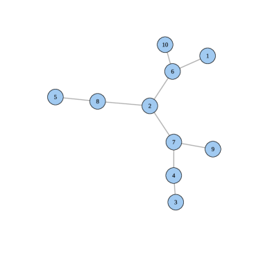
Figure 5: Tree structure for $10$-dimensional Hüsler–Reiss distribution with variogram matrix $\bm{\Gamma}_{3}$ in Table 4 used for generation of samples in Subsection 5.1

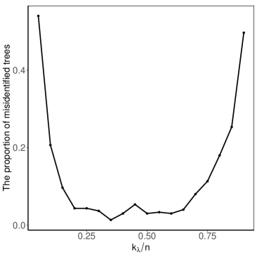
Figure 6: Proportion of misidentified trees in $300$ replications based on samples from $10$-dimensional Hüsler–Reiss distribution with variogram matrix $\bm{\Gamma}_{3}$ in Table 4 and dependence structure linked to the tree in Fig. 5

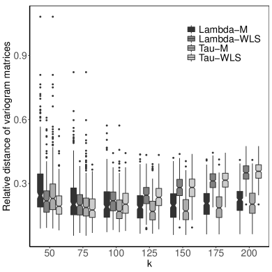
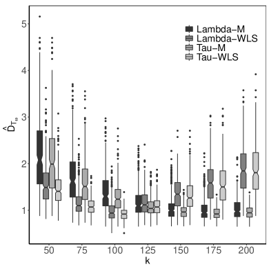
Figure 7: Boxplots of $\frac{\|\hat{\bm{\Gamma}}_{M}-\bm{\Gamma}\|_{F}}{\|\bm{\Gamma}\|_{F}}$ (left) and $\hat{D}_{\mathcal{T}_{\omega}}$ in (4.8) (right) for $10$-dimensional Hüsler–Reiss distribution with variogram matrix $\bm{\Gamma}_{4}$ based on $\hat{\mathcal{T}}_{\lambda}^{\star}$ (Lambda) and $\hat{\mathcal{T}}_{\tau}^{\star}$ (Tau), where bivariate stable tail dependence functions are fitted based on M-estimator (M) and weighted least squares estimator (WLS) at $k=50,75,\ldots,200$ ($300$ samples of size $n=1000$)

Figure 8: Boxplot of approximation errors of rare event probability in (5.3) based on $\hat{\mathcal{T}}_{\tau}^{\star}$ for $10$-dimensional Hüsler–Reiss distribution with variogram matrix $\bm{\Gamma}_{4}$, where bivariate stable tail dependence functions are fitted with M-estimator (M) and weighted least squares estimator (WLS) at $k=50,75,\ldots,200$; levels $u_{1},u_{2},u_{3}$ are taken as $0.999$ empirical marginal quantiles and $u_{j}=\infty$ for $j=4,\ldots,d$ ($300$ samples of size $n=1000$)

A.3 Additional information and analysis for Danube discharge data in Section 6

In this subsection, we list additional material related to the data analysis of daily discharges of rivers in the upper Danube basin: the information for the original discharge data in Table 5; the number of declustered excesses over the $0.9$ sample quantile of average daily discharges at $31$ gauging stations in Table 6; the tree-like river network in the upper Danube basin in Fig. 9; the maximum dependence trees $\hat{\mathcal{T}}_{\lambda}^{\star}$ and $\hat{\mathcal{T}}_{\tau}^{\star}$ selected based on $51$ years of discharge data in Fig. 10; and the parameter estimates of the generalized Pareto distribution fitted to excesses over the $0.9$ marginal empirical quantile for each gauging station in Table 7.

Table 5: The start and end recording dates and sample size of original data for Summer (June, July and August) discharges at $31$ gauging stations in the upper Danube basin

Station	Start	End	Size		Station	Start	End	Size
1	1901-06-01	2010-08-31	10120		17	1959-06-01	2013-08-31	5060
2	1901-06-01	2013-08-31	10396		18	1959-06-01	2013-08-31	5060
3	1926-06-01	2013-08-31	8096		19	1950-06-01	2013-08-31	5888
4	1924-06-01	2013-08-31	8280		20	1960-06-01	2013-08-31	4968
5	1926-06-01	2013-08-31	8096		21	1901-06-01	2013-08-31	10396
6	1901-06-01	2013-08-31	10396		22	1951-06-01	2013-08-31	5796
7	1924-06-01	2013-08-31	8280		23	1921-06-01	2013-08-31	8556
8	1924-06-01	2013-08-31	8280		24	1930-06-01	2013-08-31	7728
9	1924-06-01	2013-08-31	8280		25	1901-06-01	2013-08-31	10396
10	1954-06-01	2013-08-31	5520		26	1959-06-01	2013-08-31	5060
11	1901-06-01	2013-08-31	10396		27	1931-06-01	2013-08-31	7636
12	1901-06-01	2013-08-31	10396		28	1951-06-01	2013-08-31	5796
13	1921-06-01	2013-08-31	8556		29	1901-06-01	2013-08-31	10396
14	1926-06-01	2013-08-31	8096		30	1901-06-01	2013-08-31	10396
15	1959-06-01	2013-08-31	5060		31	1957-06-01	2013-08-31	5244
16	1959-06-01	2013-08-31	5060		–	–	–	–

Table 6: The number of declustered excesses over the $0.9$ sample quantile of average daily discharges at $31$ gauging stations in the upper Danube basin

Station	$1$	$2$	$3$	$4$	$5$	$6$	$7$	$8$	$9$	$10$	$11$
Excesses	$226$	$192$	$166$	$179$	$185$	$248$	$198$	$204$	$216$	$149$	$347$
Station	$12$	$13$	$14$	$15$	$16$	$17$	$18$	$19$	$20$	$21$	$22$
Excesses	$348$	$229$	$159$	$102$	$125$	$126$	$116$	$140$	$125$	$282$	$136$
Station	$23$	$24$	$25$	$26$	$27$	$28$	$29$	$30$	$31$	$--$	$--$
Excesses	$153$	$143$	$262$	$126$	$208$	$177$	$326$	$322$	$155$	$--$	$--$

Table 7: Parameter estimates of the generalized Pareto distribution fitted to excesses over the empirical quantile $q_{j,p}$ (rounded to the nearest integer) of daily discharges at gauging station $j=1,\ldots,31$ in the upper Danube basin

Station	$q_{j,p}$	$\hat{\sigma}_{j}$	$\hat{\vartheta}_{j}$		Station	$q_{j,p}$	$\hat{\sigma}_{j}$	$\hat{\vartheta}_{j}$
$1$	$2680$	$749.596$	$0.029$		$17$	$106$	$70.874$	$0.079$
$2$	$1040$	$387.594$	$0.017$		$18$	$75$	$72.553$	$0.040$
$3$	$715$	$278.147$	$0.074$		$19$	$57$	$54.261$	$0.161$
$4$	$715$	$289.252$	$0.047$		$20$	$236$	$142.385$	$0.098$
$5$	$598$	$232.214$	$0.057$		$21$	$193$	$96.663$	$0.036$
$6$	$577$	$225.447$	$0.027$		$22$	$173$	$91.849$	$0.016$
$7$	$553$	$252.046$	$-0.025$		$23$	$58$	$40.197$	$0.202$
$8$	$309$	$136.322$	$0.046$		$24$	$44$	$33.902$	$0.199$
$9$	$270$	$136.070$	$0.054$		$25$	$51$	$41.917$	$0.243$
$10$	$212$	$120.944$	$-0.016$		$26$	$45$	$29.339$	$0.413$
$11$	$114$	$77.116$	$0.030$		$27$	$38$	$24.371$	$0.409$
$12$	$54$	$35.780$	$0.032$		$28$	$94$	$65.412$	$0.249$
$13$	$1630$	$579.764$	$0.123$		$29$	$90$	$66.082$	$0.139$
$14$	$315$	$120.868$	$0.124$		$30$	$578$	$275.008$	$0.116$
$15$	$296$	$123.116$	$0.089$		$31$	$544$	$256.610$	$0.205$
$16$	$162$	$103.409$	$0.092$		$--$	$--$	$--$	$--$

Figure 9: Tree-like structure of the river network in the upper Danube basin. Each node represents a numbered gauging station along the rivers and water flows toward gauging station $1$.

Figure 10: Maximum dependence trees $\hat{\mathcal{T}}_{\lambda}^{\star}$ (left) and $\hat{\mathcal{T}}_{\tau}^{\star}$ (right) in (4.3) selected based on the declustered excesses of $51$ years of average daily discharges at $31$ gauging stations in the upper Danube basin. The empty nodes are those which have different neighbours from the tree structure of the river network in Fig. 9.

References

- Asadi et al., (2015) Asadi, P., Davison, A. C., & Engelke, S. (2015). Extremes on river networks. The Annals of Applied Statistics, 9(4), 2023–2050.
- Asenova et al., (2021) Asenova, S., Mazo, G., & Segers, J. (2021). Inference on extremal dependence in the domain of attraction of a structured Hüsler–Reiss distribution motivated by a markov tree with latent variables. Extremes, 24, 461–500.
- Asenova & Segers, (2021) Asenova, S. & Segers, J. (2021). Extremes of Markov random fields on block graphs. ArXiv:2112.04847.
- Ballani & Schlather, (2011) Ballani, F. & Schlather, M. (2011). A construction principle for multivariate extreme value distributions. Biometrika, 98(3), 633–645.
- Beirlant et al., (2016) Beirlant, J., Escobar-Bach, M., Goegebeur, Y., & Guillou, A. (2016). Bias-corrected estimation of stable tail dependence function. Journal of Multivariate Analysis, 143, 453–466.
- Beirlant et al., (2004) Beirlant, J., Goegebeur, Y., Segers, J., Teugels, J., De Waal, D., & Ferro, C. (2004). Statistics of Extremes: Theory and Applications. John Wiley & Sons.
- Boldi & Davison, (2007) Boldi, M.-O. & Davison, A. C. (2007). A mixture model for multivariate extremes. Journal of the Royal Statistical Society: Series B (Statistical Methodology), 69(2), 217–229.
- Bücher et al., (2014) Bücher, A., Segers, J., & Volgushev, S. (2014). When uniform weak convergence fails: empirical processes for dependence functions and residuals via epi- and hypographs. The Annals of Statistics, 42(4), 1598–1634.
- Chow & Liu, (1968) Chow, C.-S. & Liu, C. (1968). Approximating discrete probability distributions with dependence trees. IEEE Transactions on Information Theory, 14(3), 462–467.
- Coles, (2001) Coles, S. G. (2001). An Introduction to Statistical Modelling of Extreme Values. London: Springer.
- Coles & Tawn, (1991) Coles, S. G. & Tawn, J. A. (1991). Modelling extreme multivariate events. Journal of the Royal Statistical Society: Series B (Statistical Methodology), 53(2), 377–392.
- Cooley et al., (2010) Cooley, D., Davis, R. A., & Naveau, P. (2010). The pairwise beta distribution: A flexible parametric multivariate model for extremes. Journal of Multivariate Analysis, 101, 2103–2117.
- Davison & Huser, (2015) Davison, A. C. & Huser, R. (2015). Statistics of extremes. Annual Review of Statistics and Its Application, 2(1), 203–235.
- Davison et al., (2012) Davison, A. C., Padoan, S., & Ribatet, M. (2012). Statistical modelling of spatial extremes. Statistical Science, 27, 161–186.
- de Haan & Ferreira, (2006) de Haan, L. & Ferreira, A. (2006). Extreme Value Theory: An Introduction. New York: Springer.
- Deheuvels, (1991) Deheuvels, P. (1991). On the limiting behavior of the pickands estimator for bivariate extreme-value distributions. Statistics & Probability Letters, 12(5), 429–439.
- Drees & Huang, (1998) Drees, H. & Huang, X. (1998). Best attainable rates of convergence for estimators of the stable tail dependence function. Journal of Multivariate Analysis, 64(1), 25–46.
- Einmahl et al., (2016) Einmahl, J. H., Kiriliouk, A., Krajina, A., & Segers, J. (2016). An M-estimator of spatial tail dependence. Journal of the Royal Statistical Society: Series B (Statistical Methodology), 78(Part 1), 275–298.
- Einmahl et al., (2018) Einmahl, J. H., Kiriliouk, A., & Segers, J. (2018). A continuous updating weighted least squares estimator of tail dependence in high dimensions. Extremes, 21(2), 205–233.
- Einmahl et al., (2008) Einmahl, J. H., Krajina, A., & Segers, J. (2008). A method of moments estimator of tail dependence. Bernoulli, 14(4), 1003–1026.
- Einmahl et al., (2012) Einmahl, J. H., Krajina, A., & Segers, J. (2012). An M-estimator for tail dependence in arbitrary dimensions. The Annals of Statistics, 40(3), 1764–1793.
- Einmahl et al., (2001) Einmahl, J. H., Piterbarg, V. I., & De Haan, L. (2001). Nonparametric estimation of the spectral measure of an extreme value distribution. The Annals of Statistics, 29(5), 1401–1423.
- Einmahl & Segers, (2009) Einmahl, J. H. & Segers, J. (2009). Maximum empirical likelihood estimation of the spectral measure of an extreme-value distribution. The Annals of Statistics, 37(5B), 2953–2989.
- Engelke & Hitz, (2020) Engelke, S. & Hitz, A. S. (2020). Graphical models for extremes. Journal of the Royal Statistical Society: Series B (Statistical Methodology), 82(4), 871–932.
- Engelke et al., (2019) Engelke, S., Hitz, A. S., & Gnecco, N. (2019). graphicalExtremes: Statistical Methodology for Graphical Extreme Value Models. R package version 0.1.0.
- Engelke & Ivanovs, (2021) Engelke, S. & Ivanovs, J. (2021). Sparse structures for multivariate extremes. Annual Review of Statistics and Its Application, 8, 241–270.
- Engelke & Volgushev, (2020) Engelke, S. & Volgushev, S. (2020). Structure learning for extremal tree models. ArXiv:2012.06179.
- Gissibl & Klüppelberg, (2018) Gissibl, N. & Klüppelberg, C. (2018). Max-linear models on directed acyclic graphs. Bernoulli, 24(4A), 2693–2720.
- Gissibl et al., (2018) Gissibl, N., Klüppelberg, C., & Otto, M. (2018). Tail dependence of recursive max-linear models with regularly varying noise variables. Econometrics and Statistics, 6, 149–167.
- Gumbel, (1960) Gumbel, E. J. (1960). Bivariate exponential distributions. Journal of the American Statistical Association, 55(292), 698–707.
- Hall, (1935) Hall, P. (1935). On representatives of subsets. Jounal of the London Mathematical Society, s1-10(1), 26–30.
- Hanson et al., (2017) Hanson, T. E., de Carvalho, M., & Chen, Y. (2017). Bernstein polynomial angular densities of multivariate extreme value distributions. Statistics & Probability Letters, 128, 60–66.
- Horváth et al., (2020) Horváth, G., Kovács, E., Molontay, R., & Nováczki, S. (2020). Copula-based anomaly scoring and localization for large-scale, high-dimensional continuous data. ACM Transactions on Intelligent Systems and Technology (TIST), 11(3), 1–26.
- Huang, (1992) Huang, X. (1992). Statistics of Bivariate Extremes. PhD thesis, Erasmus University.
- Hüsler & Reiss, (1989) Hüsler, J. & Reiss, R.-D. (1989). Maxima of normal random vectors: between independence and complete dependence. Statistics & Probability Letters, 7(4), 283–286.
- Kiriliouk et al., (2019) Kiriliouk, A., Rootzén, H., Segers, J., & Wadsworth, J. L. (2019). Peaks over thresholds modeling with multivariate generalized pareto distributions. Technometrics, 61(1), 123–135.
- Kiriliouk et al., (2018) Kiriliouk, A., Segers, J., & Tafakori, L. (2018). An estimator of the stable tail dependence function based on the empirical beta copula. Extremes, 21(4), 581–600.
- Kotz & Nadarajah, (2000) Kotz, S. & Nadarajah, S. (2000). Extreme Value Distributions: Theory and Applications. World Scientific.
- Narasimhan et al., (2019) Narasimhan, B., Johnson, S. G., Hahn, T., Bouvier, A., & Kiêu, K. (2019). cubature: Adaptive Multivariate Integration over Hypercubes. R package version 2.0.4.
- Papadimitriou & Steiglitz, (1998) Papadimitriou, C. H. & Steiglitz, K. (1998). Combinatorial Optimization: Algorithms and Complexity. Courier Corporation.
- Papastathopoulos & Strokorb, (2016) Papastathopoulos, I. & Strokorb, K. (2016). Conditional independence among max-stable laws. Statistics & Probability Letters, 108, 9–15.
- Peng & Qi, (2008) Peng, L. & Qi, Y. (2008). Bootstrap approximation of tail dependence function. Journal of Multivariate Analysis, 99(8), 1807–1824.
- Prim, (1957) Prim, R. (1957). Shortest connection networks and some generalizations. The Bell System Technical Journal, 36(6), 1389–1401.
- Resnick, (1987) Resnick, S. I. (1987). Extreme Values, Regular Variation, and Point Processes. Springer-Verlag, New York.
- Schmidt & Stadtmüller, (2006) Schmidt, R. & Stadtmüller, U. (2006). Non-parametric estimation of tail dependence. Scandinavian Journal of Statistics, 33(2), 307–335.
- Segers, (2020) Segers, J. (2020). One-versus multi-component regular variation and extremes of Markov trees. Advances in Applied Probability, 52(3), 855–878.
- Tawn, (1990) Tawn, J. A. (1990). Modelling multivariate extreme value distributions. Biometrika, 77(2), 245–253.
- van der Vaart, (1998) van der Vaart, A. W. (1998). Asymptotic Statistics. Cambridge: Cambridge University Press.