Quantum adiabaticity in many-body systems and almost-orthogonality in complementary subspace

Abstract

We study why in quantum many-body systems the adiabatic fidelity and the overlap between the initial state and instantaneous ground states have nearly the same values in many cases. We elaborate on how the problem may be explained by an interplay between the two intrinsic limits of many-body systems: the limit of small values of evolution parameter and the limit of large system size. In the former case, conventional perturbation theory provides a natural explanation. In the latter case, a crucial observation is that pairs of vectors lying in the complementary Hilbert space of the initial state are almost orthogonal. Our general findings are illustrated with a driven Rice-Mele model and a driven interacting Kitaev chain model, two paradigmatic models of driven many-body systems.

I Introduction

In the modern era of quantum technologies, it is crucial to prepare and manipulate quantum states with precision. For this purpose, various approximations based on the quantum adiabatic theorem (QAT) Born (1927); Born and Fock (1928); Kato (1950); Messiah (2014) are widely used. Examples of applications include adiabatic quantum transport Thouless (1983); Berry (1984); Avron et al. (1988); Avron (1995), adiabatic quantum computation Farhi et al. (2000); Roland and Cerf (2002); Albash and Lidar (2018), and adiabatic quantum state manipulation Ivanov (2001); Nayak et al. (2008); Hamma and Lidar (2008); Alicea et al. (2011); Halperin et al. (2012); van Heck et al. (2012) and preparation Aspuru-Guzik et al. (2005); Aharonov and Ta‐Shma (2007); Wecker et al. (2015); Reiher et al. (2017); Wan and Kim (2020); Coello Pérez et al. (2022). Adiabatic evolution refers to the evolution of a quantum system whose time-evolved state remains close to its instantaneous eigenstate. A well-known adiabatic criterion Messiah (2014); Jansen et al. (2007) is that the rate of change of the time-dependent Hamiltonian must be much smaller than certain non-negative powers of the minimum energy gap of the Hamiltonian. Although calculating energy gaps is often possible for systems with a small Hilbert space or for exactly solvable models, it is generically difficult for many-body systems with a big Hilbert space. Alternatively, the formalism of shortcuts to adiabaticity (STA) promises to give the same adiabatic results as those provided by the QAT but without requiring slow driving Demirplak and Rice (2003); Berry (2009); Chen et al. (2010); Torrontegui et al. (2013); Jarzynski (2013); del Campo (2013); Bukov et al. (2019); Guéry-Odelin et al. (2019). Yet, since counterdiabatic terms in many-body systems are not necessarily local in space del Campo et al. (2012); Takahashi (2013); Saberi et al. (2014); Sels and Polkovnikov (2017), there are circumstances in which the STA approach is not useful for practical purposes.

Instead, a complementary bottom-up approach considers how the fidelity (termed adiabatic fidelity) between the time-evolved states and the instantaneous eigenstates deviates from unity under dynamical evolution. However, for quantum many-body systems, obtaining time-evolved states and instantaneous eigenstates by solving the many-body Schrödinger equation and eigenvalue equation may be a difficult task. It then raises the question of whether one can estimate the adiabatic fidelity without solving equations from scratch.

The approach initiated by Ref. Lychkovskiy et al. (2017) and extended in Ref. Chen and Cheianov (2022) is that the adiabatic fidelity can be estimated by exploiting a many-body nature of the problem — generalized orthogonality catastrophe (GOC), and a fundamental inequality for the evolution of unitary dynamics in Hilbert spaces — quantum speed limit (QSL). The GOC refers to the property that the fidelity between instantaneous eigenstates and the initial state decays exponentially as the system size and the value of the evolution parameter increase Lychkovskiy et al. (2017), whereas the QSL sets an intrinsic limit on how fast the time-evolved state can deviate from the initial state Mandelstam and Tamm (1945); Vaidman (1992); Pfeifer (1993a, b); Pfeifer and Fröhlich (1995); Deffner and Campbell (2017); Gong and Hamazaki (2022).

In Ref. Chen and Cheianov (2022), a novel vector decomposition method (which will be reviewed in Sec. II.2) was developed to enrich the program of estimating the adiabatic fidelity using the GOC and the QSL. Although the results obtained in Ref. Chen and Cheianov (2022) provide improved estimates compared to that of Ref. Lychkovskiy et al. (2017), there remains a question as to why the numerical value of the adiabatic fidelity and the GOC are almost the same in many situations (e.g., when the value of the evolution parameter is small, or when the system size is large). The primary purpose of the present work is to address this question. We find that the closeness between the adiabatic fidelity and the GOC is a consequence of the interplay between the following two facts. First, in the region of small values of the evolution parameter, the time-evolved state is still close to the initial state. Hence, the closeness between the adiabatic fidelity and the GOC can be naturally understood. Second, when the evolution parameter continues to increase, the perturbation argument is insufficient. For this region, the closeness issue may be explained by the almost-orthogonality of random vectors occurring in the complementary subspace of the initial state.

The rest of this paper is organized as follows. After reviewing the basic formalism in Sec. II, we consider a limiting case in Sec. III in which the essential elements for addressing the proposed question are exposed. We then derive a set of useful triangle-type inequality in Sec. IV. In Sec. V, we illustrate our general results with a driven Rice-Mele model. Implication, further example, and summary are presented in Sec. VI, Sec. VII, and Sec. VIII, respectively. Supplemental Material (SM) includes some technical details.

II Preliminaries

II.1 Setup

We begin by defining notations and terminologies. Consider a time-dependent Hamiltonian $H^{\,}_{\lambda}$ with $\lambda=\lambda(t)$ being an explicit function of time $t$. Using $\lambda$ in place of $t$ as the evolution parameter, the Schrödinger equation for the time-evolved state $|\Psi^{\,}_{\lambda}\rangle$ reads

$$\mathrm{i}\Gamma\partial^{\,}_{\lambda}|\Psi^{\,}_{\lambda}\rangle=H^{\,}_{\lambda}|\Psi^{\,}_{\lambda}\rangle\quad\text{with}\quad|\Psi^{\,}_{0}\rangle=|\Phi^{\,}_{0}\rangle,$$ (1)

where $\Gamma\,\raisebox{0.85pt}{.}\raisebox{2.85pt}{.}\!\!=\,\partial^{\,}_{t}\lambda(t)$ being the driving rate and we assume that the initial state, $|\Psi^{\,}_{0}\rangle,$ is in the ground state of the Hamiltonian $H^{\,}_{\lambda}$ at $\lambda=0,$ $|\Phi^{\,}_{0}\rangle.$ For generic values of $\lambda,$ the instantaneous ground state of the Hamiltonian $H^{\,}_{\lambda}$ is the solution to the eigenvalue problem,

$$H^{\,}_{\lambda}|\Phi^{\,}_{\lambda}\rangle=E^{\,}_{\mathrm{GS},\lambda}|\Phi^{\,}_{\lambda}\rangle$$ (2)

with $E^{\,}_{\mathrm{GS},\lambda}$ being the $\lambda$-dependent ground state energy. To quantify the distance between $|\Psi^{\,}_{\lambda}\rangle$ and $|\Phi^{\,}_{\lambda}\rangle,$ one introduces the quantum fidelity $\mathcal{F}(\lambda)$ between them,

$$\mathcal{F}(\lambda)\,\raisebox{0.85pt}{.}\raisebox{2.85pt}{.}\!\!=\,|\langle\Phi^{\,}_{\lambda}|\Psi^{\,}_{\lambda}\rangle|^{2}.$$ (3)

Let $\mathcal{C}(\lambda)$ be the overlap between the initial ground state $|\Phi^{\,}_{0}\rangle$ and the instantaneous ground state $|\Phi^{\,}_{\lambda}\rangle$ for an arbitrary value of $\lambda$,

$$\mathcal{C}(\lambda)\,\raisebox{0.85pt}{.}\raisebox{2.85pt}{.}\!\!=\,|\langle\Phi^{\,}_{\lambda}|\Phi^{\,}_{0}\rangle|^{2}.$$ (4)

For a large class of many-body systems $\mathcal{C}(\lambda)$ has an asymptotic form $\mathcal{C}(\lambda)\sim e^{-C^{\,}_{N}\lambda^{2}}$ under the limit of large system size, i.e. $N\to\infty$ Lychkovskiy et al. (2017). Generalized orthogonality catastrophe, renaissance of Anderson’s orthogonality catastrophe Anderson (1967); Gebert et al. (2014), takes place if the exponent $C^{\,}_{N}\to\infty$ as $N\to\infty.$ The scaling form of the exponent $C^{\,}_{N}$ depends on the type of driving, space dimensions, and whether the energy gap is present or not Lychkovskiy et al. (2017).

At any value of $\lambda,$ we are given three vectors: $|\Phi^{\,}_{\lambda}\rangle$, $|\Psi^{\,}_{\lambda}\rangle$, and $|\Phi^{\,}_{0}\rangle.$ There are three ways to construct overlaps between any two of the three vectors. We have already mentioned two kinds of the overlaps, namely, the adiabatic fidelity $\mathcal{F}(\lambda)$ (3) and the ground state overlap $\mathcal{C}(\lambda)$ (4). The remaining overlap, $|\langle\Psi^{\,}_{\lambda}|\Phi^{\,}_{0}\rangle|^{2},$ can be utilized to define the distance between the initial state $|\Phi^{\,}_{0}\rangle$ and the time-evolved state $|\Phi^{\,}_{\lambda}\rangle$ through the Bures angle $\theta(\lambda)\in[0,\pi/2]$,

$$\theta(\lambda)\,\raisebox{0.85pt}{.}\raisebox{2.85pt}{.}\!\!=\,\arccos|\langle\Psi^{\,}_{\lambda}|\Phi^{\,}_{0}\rangle|.$$ (5)

An inequality of quantum speed limit of the Mandelstam-Tamm type Mandelstam and Tamm (1945); Vaidman (1992); Pfeifer (1993a, b); Pfeifer and Fröhlich (1995); Deffner and Campbell (2017); Gong and Hamazaki (2022) sets an upper bound on the Bures angle $\theta(\lambda)$ (5),

$$\theta(\lambda)\leq\min\left(\mathcal{R}(\lambda),\frac{\pi}{2}\right)\,=\!\!\raisebox{0.85pt}{.}\raisebox{2.85pt}{.}\,\widetilde{\mathcal{R}}(\lambda),$$ (6a)

$$\text{where}\quad\mathcal{R}(\lambda)\,\raisebox{0.85pt}{.}\raisebox{2.85pt}{.}\!\!=\,\int^{\lambda}_{0}\frac{\mathrm{d}\lambda^{\prime}}{|\Gamma(\lambda^{\prime})|}\sqrt{\langle H^{2}_{\lambda^{\prime}}\rangle^{\,}_{0}-\langle H^{\,}_{\lambda^{\prime}}\rangle^{2}_{0}},$$ (6b)

with $$\langle\cdots\rangle^{\,}_{0}\,\raisebox{0.85pt}{.}\raisebox{2.85pt}{.}\!\!=\,\langle\Phi^{\,}_{0}|\cdots|\Phi^{\,}_{0}\rangle.$$

In the present work, we shall pay particular attention to the time-dependent Hamiltonian $H^{\,}_{\lambda}$ of the following form:

$$H^{\,}_{\lambda}=H^{\,}_{0}+\lambda V,$$ (7)

for which the function $\mathcal{R}(\lambda)$ (6b) with a positive constant driving rate $\Gamma$ reads

$$\mathcal{R}(\lambda)=\frac{\lambda^{2}}{2\Gamma}\delta V^{\,}_{N}\quad\text{with}\quad\delta V^{\,}_{N}\,\raisebox{0.85pt}{.}\raisebox{2.85pt}{.}\!\!=\,\sqrt{\langle V^{2}\rangle^{\,}_{0}-\langle V\rangle^{2}_{0}}.$$ (8)

II.2 Orthogonal decomposition

We now review the formalism developed in Ref. Chen and Cheianov (2022) but adopt a more compact notation. Define $P=|\Phi^{\,}_{0}\rangle\langle\Phi^{\,}_{0}|$ as a projector onto the initial state and $Q=\mathbb{I}-P$ as the complementary projector. By definition, $P^{2}=P,Q^{2}=Q,$ and $PQ=QP=0.$ Consider the following orthogonal decompositions for the time-evolved state $|\Psi^{\,}_{\lambda}\rangle$ and the instantaneous ground state $|\Phi^{\,}_{\lambda}\rangle$,

$$|\Psi^{\,}_{\lambda}\rangle=P|\Psi^{\,}_{\lambda}\rangle+Q|\Psi^{\,}_{\lambda}\rangle,$$ (9a)

$$|\Phi^{\,}_{\lambda}\rangle=P|\Phi^{\,}_{\lambda}\rangle+Q|\Phi^{\,}_{\lambda}\rangle.$$ (9b)

Notice that, by the construction of Eq. (9), the following relations hold (here, $\||\cdot\rangle\|\,\raisebox{0.85pt}{.}\raisebox{2.85pt}{.}\!\!=\,\sqrt{\langle\cdot|\cdot\rangle}$),

$$\|P|\Psi^{\,}_{\lambda}\rangle\|=|\langle\Phi^{\,}_{0}|\Psi^{\,}_{\lambda}\rangle|=\cos\theta(\lambda),$$ (10a)

$$\|Q|\Psi^{\,}_{\lambda}\rangle\|=\sqrt{1-|\langle\Phi^{\,}_{0}|\Psi^{\,}_{\lambda}\rangle|^{2}}=\sin\theta(\lambda),$$ (10b)

$$\|P|\Phi^{\,}_{\lambda}\rangle\|=|\langle\Phi^{\,}_{0}|\Phi^{\,}_{\lambda}\rangle|=\sqrt{C(\lambda)},$$ (10c)

$$\|Q|\Phi^{\,}_{\lambda}\rangle\|=\sqrt{1-|\langle\Phi^{\,}_{0}|\Phi^{\,}_{\lambda}\rangle|^{2}}=\sqrt{1-\mathcal{C}(\lambda)},$$ (10d)

where the Bures angle $$\theta(\lambda) \mathcal{C}(\lambda)$$ and the ground state overlap is introduced in Eqs. (5) and (4), respectively.

The two vectors, $Q|\Psi^{\,}_{\lambda}\rangle$ and $Q|\Phi^{\,}_{\lambda}\rangle$, are not normalized; we defined the corresponding normalized vectors as

$$|\Phi^{\perp}_{0}(\lambda)\rangle\,\raisebox{0.85pt}{.}\raisebox{2.85pt}{.}\!\!=\,\frac{Q|\Psi^{\,}_{\lambda}\rangle}{\|Q|\Psi^{\,}_{\lambda}\rangle\|},\quad|\widetilde{\Phi}^{\perp}_{0}(\lambda)\rangle\,\raisebox{0.85pt}{.}\raisebox{2.85pt}{.}\!\!=\,\frac{Q|\Phi^{\,}_{\lambda}\rangle}{\|Q|\Phi^{\,}_{\lambda}\rangle\|},$$ (11)

where the superscript $\perp$ indicates that these two normalized vectors are orthogonal to the initial state $|\Phi^{\,}_{0}\rangle.$ We introduce $\mathcal{D}(\lambda)$ to denote the overlap between the two normalized vectors, $|\Phi^{\perp}_{0}(\lambda)\rangle$ and $|\widetilde{\Phi}^{\perp}_{0}(\lambda)\rangle$,

$$\mathcal{D}(\lambda)\,\raisebox{0.85pt}{.}\raisebox{2.85pt}{.}\!\!=\, \,|\langle\Phi^{\perp}_{0}(\lambda)|\widetilde{\Phi}^{\perp}_{0}(\lambda)\rangle|^{2},$$ (12)

and $\mathcal{D}^{\,}_{\mathrm{un}}(\lambda)$ to denote the overlap between the two unnormalized vectors, $Q|\Psi^{\,}_{\lambda}\rangle$ and $Q|\Phi^{\,}_{\lambda}\rangle$,

$$\mathcal{D}^{\,}_{\mathrm{un}}(\lambda)\,\raisebox{0.85pt}{.}\raisebox{2.85pt}{.}\!\!=\,\left|\langle\Psi^{\,}_{\lambda}|Q|\Phi^{\,}_{\lambda}\rangle\right|^{2}.$$ (13)

Note that the two overlaps, $\mathcal{D}(\lambda)$ and $\mathcal{D}^{\,}_{\mathrm{un}}(\lambda)$, are not independent. They are related through

$$\sqrt{\mathcal{D}^{\,}_{\mathrm{un}}(\lambda)} =\sin\theta(\lambda)\sqrt{1-\mathcal{C}(\lambda)}\sqrt{\mathcal{D}(\lambda)}.$$ (14)

Both $\mathcal{D}(\lambda)$ and $\mathcal{D}^{\,}_{\mathrm{un}}(\lambda)$ play important roles in the following discussion.

Our aim is to bound the difference between the adiabatic fidelity $\mathcal{F}(\lambda)$ (3) and the ground state overlap $\mathcal{C}(\lambda)$ (4). It was found in our recent work Chen and Cheianov (2022) [see also Supplemental Material (SM) S1 for an alternative derivation] that the difference between $\mathcal{F}(\lambda)$ and $\mathcal{C}(\lambda)$ obeys the following inequality

$$\left|\mathcal{F}(\lambda)-\mathcal{C}(\lambda)\right|\leq \,\left|-\sin^{2}\theta(\lambda)\mathcal{C}(\lambda)+\mathcal{D}^{\,}_{\mathrm{un}}(\lambda)\right|$$

$$+2\cos\theta(\lambda)\sqrt{\mathcal{C}(\lambda)}\sqrt{\mathcal{D}^{\,}_{\mathrm{un}}(\lambda)},$$ (15)

where $\mathcal{D}^{\,}_{\mathrm{un}}(\lambda)$ is defined in Eq. (14). To make further progress, the strategy made in Ref. Chen and Cheianov (2022) is to replace the normalized overlap $\mathcal{D}(\lambda)$ in Eq. (14) by its trivial upper bound 1, i.e., $\mathcal{D}(\lambda)\leq 1,$ which renders the unnormalized overlap $\mathcal{D}^{\,}_{\mathrm{un}}(\lambda)$ (14) bounded from above as follows

$$\sqrt{\mathcal{D}^{\,}_{\mathrm{un}}(\lambda)}\leq\sin^{\,}\theta(\lambda)\sqrt{1-\mathcal{C}(\lambda)}.$$ (16)

The idea of adopting the upper bound, $\mathcal{D}(\lambda)\leq 1,$ is that since presumably we have no information about the overlap between the two normalized vectors, $|\Phi^{\perp}_{0}(\lambda)\rangle$ and $|\widetilde{\Phi}^{\perp}_{0}(\lambda)\rangle$ (11), we may simply replace their overlap by the trivial upper bound of their overlap. Applying the upper bound (16) to the inequality (15) yields

$$\left|\mathcal{F}(\lambda)-\mathcal{C}(\lambda)\right|\,\leq\, \sin^{2}\theta\left|1-2\mathcal{C}\right|$$

$$+\sin(2\theta)\sqrt{\mathcal{C}}\sqrt{1-\mathcal{C}}.$$ (17)

Upon applying the quantum speed limit (6) to bound the Bures angle $\theta(\lambda)$ in Eq. (17), the following improved inequality is obtained by Ref. Chen and Cheianov (2022),

$$\left|\mathcal{F}(\lambda)-\mathcal{C}(\lambda)\right|\;\leq\;f(\lambda),\quad f(\lambda)\,\raisebox{0.85pt}{.}\raisebox{2.85pt}{.}\!\!=\,f^{\,}_{1}(\lambda)+f^{\,}_{2}(\lambda),$$ (18a)

$$f^{\,}_{1}(\lambda)\,\raisebox{0.85pt}{.}\raisebox{2.85pt}{.}\!\!=\,\sin^{2}\widetilde{\mathcal{R}}(\lambda)\left|1-2\mathcal{C}(\lambda)\right|,$$ (18b)

$$f^{\,}_{2}(\lambda)\,\raisebox{0.85pt}{.}\raisebox{2.85pt}{.}\!\!=\,\sin(2\widetilde{\widetilde{\mathcal{R}}}(\lambda))\sqrt{\mathcal{C}(\lambda)}\sqrt{1-\mathcal{C}(\lambda)},$$ (18c)

where $$\widetilde{\mathcal{R}}(\lambda) \widetilde{\widetilde{\mathcal{R}}}(\lambda)$$ is defined in Eq. (6) and is defined as

$$\widetilde{\widetilde{\mathcal{R}}}(\lambda)\,\raisebox{0.85pt}{.}\raisebox{2.85pt}{.}\!\!=\,\min\left(\mathcal{R}(\lambda),\frac{\pi}{4}\right).$$ (18d)

Although the inequality (18) improves the inequality found in Ref. Lychkovskiy et al. (2017), i.e., $\left|\mathcal{F}(\lambda)-\mathcal{C}(\lambda)\right|\leq\widetilde{\mathcal{R}}(\lambda),$ there is still a question of why the value of the adiabatic fidelity $\mathcal{F}(\lambda)$ and the ground state overlap $\mathcal{C}(\lambda)$ are nearly identical when (i) the system size $N$ is sufficiently large (say, $N\geq 100$), or (ii) the evolution parameter $\lambda$ is small for any system size. In this work, we shall address this question using the orthogonal decomposition formalism presented in this Section.

III A motivating limit and interpretations

By inspecting Eq. (15), one finds that the least controlled piece is the unnormalized overlap $\mathcal{D}^{\,}_{\mathrm{un}}(\lambda)$ (13), which contains two factors [see Eq. (14)], namely, $\sin\theta(\lambda)\sqrt{1-\mathcal{C}(\lambda)}$ and $\sqrt{D(\lambda)}$. Among them, the trivial upper bound of $\mathcal{D}(\lambda)$ is employed in Ref. Chen and Cheianov (2022) to obtain universal upper bounds on $|\mathcal{F}(\lambda)-\mathcal{C}(\lambda)|$ [see Eq. (17)]. Therefore, the reason why the inequality (18) is insufficient to explain the smallness of $|\mathcal{F}(\lambda)-\mathcal{C}(\lambda)|$ may be due to the use of the trivial upper bound, $\mathcal{D}(\lambda)\leq 1.$ To justify this claim, we simply look at the extreme limit:

$$\mathcal{D}^{\,}_{\mathrm{un}}(\lambda)\to 0.$$ (19)

We will elaborate on the orthogonal relation (19) later. For the moment, let us examine consequences of it. Imposing the orthogonality limit (19) to the defining equations (9), the calculation of $|\mathcal{F}(\lambda)-\mathcal{C}(\lambda)|$ is fairly simple. First, we find from Eqs. (9) and (10) that

$$\mathcal{F}(\lambda)\to\cos^{2}\theta(\lambda)\mathcal{C}(\lambda).$$ (20)

It then follows that

$$|\mathcal{F}(\lambda)-\mathcal{C}(\lambda)|\to\sin^{2}\theta(\lambda)\,\mathcal{C}(\lambda)\,\leq\,\sin^{2}\widetilde{\mathcal{R}}(\lambda)\,\mathcal{C}(\lambda)$$ (21)

after using the quantum speed limit (6). The inequality (21) should be compared with that of Eq. (18) in which only part of $f^{\,}_{1}(\lambda)$ (18a) is retained on the right side of Eq. (21), providing a stronger upper bound on $|\mathcal{F}(\lambda)-\mathcal{C}(\lambda)|.$

The orthogonality ansatz (19), in view of Eq. (14), can be fulfilled by either

$$\text{(i)}\;\sin\theta(\lambda)\sqrt{1-\mathcal{C}(\lambda)}\to 0\quad\text{or}\quad\text{(ii)}\;\sqrt{D(\lambda)}\to 0.$$ (22)

Case (i) is satisfied if $\lambda$ is small. This is anticipated since if $\lambda$ is small, one expects that the Bures angle $\theta(\lambda)$ is still small as well, while both $\mathcal{C}(\lambda)$ and $\mathcal{D}(\lambda)$ remain close to one. We shall provide an explicit calculation from perturbative expansion in $\lambda$ shortly. As we shall see later, case (ii) is a manifestation of almost-orthogonality occurring in the complementary subspace of the initial state $|\Phi^{\,}_{0}\rangle.$ We now elaborate on the two cases of Eq. (22) in turn.

III.1 Insights from perturbative expansion in $\lambda$

We here provide a further explanation for the case (i) of Eq. (22). The goal is to solve the instantaneous eigenvalue equation (2) and the time-dependent Schrödinger equation (1) perturbatively in $\lambda$ with the Hamiltonian $H^{\,}_{\lambda}$ (7), given the eigenvalue equation of $H^{\,}_{0},$

$$H^{\,}_{0}|\chi^{\,}_{n}\rangle=\varepsilon^{\,}_{n}|\chi^{\,}_{n}\rangle,$$ (23)

where $\{|\chi^{\,}_{n}\rangle\}$ is a complete set of orthonormal eigenstates of $H^{\,}_{0}$ with $|\chi^{\,}_{0}\rangle\equiv|\Psi^{\,}_{0}\rangle$ being its ground state and $n\in\{0,1,\cdots\}$ labels different eigenstates. One finds (refer to SM S2 for details) that, up to order $\lambda^{2},$ the adiabatic fidelity $\mathcal{F}(\lambda)$ (3) and the ground state overlap $\mathcal{C}(\lambda)$ (4) are identical and are independent of the driving rate $\Gamma$,

$$\mathcal{F}(\lambda)\simeq\mathcal{C}(\lambda)=1-\lambda^{2}\sum^{\,}_{n\neq 0}\frac{|V^{\,}_{n0}|^{2}}{(\varepsilon^{\,}_{0}-\varepsilon^{\,}_{n})^{2}}+\mathcal{O}(\lambda^{3}),$$ (24)

where the matrix element $V^{\,}_{nm}\,\raisebox{0.85pt}{.}\raisebox{2.85pt}{.}\!\!=\,\langle\chi^{\,}_{n}|V|\chi^{\,}_{m}\rangle.$ The difference between $\mathcal{F}(\lambda)$ and $\mathcal{C}(\lambda)$ appears at order $\lambda^{3},$ $\mathcal{F}(\lambda)-\mathcal{C}(\lambda)=-\lambda^{3}V^{\,}_{00}\varepsilon^{\,}_{0}/\Gamma^{2}+\cdots.$ Leading order contributions for various quantities can also be obtained,

$$\sin\theta(\lambda)=\frac{\lambda^{2}}{2\Gamma}\Big{(}\sum^{\,}_{n\neq 0}|V^{\,}_{n0}|^{2}\Big{)}^{1/2}+\mathcal{O}(\lambda^{3}),$$ (25a)

$$\sqrt{\mathcal{D}^{\,}_{\mathrm{un}}(\lambda)}=\frac{\lambda^{3}}{2\Gamma}\sum^{\,}_{n\neq 0}\frac{|V^{\,}_{n0}|^{2}}{\varepsilon^{\,}_{n}-\varepsilon^{\,}_{0}}+\mathcal{O}(\lambda^{4}),$$ (25b)

$$\sin\theta(\lambda)\sqrt{1-\mathcal{C}(\lambda)}=\mathcal{O}(\lambda^{3}),$$ (25c)

$$\sqrt{\mathcal{D}(\lambda)}=\mathcal{O}(1).$$ (25d)

We see that, for small $\lambda$, $\sqrt{\mathcal{D}^{\,}_{\mathrm{un}}(\lambda)}$ (14) is of order $\lambda^{3},$ which is attributed to the same order of small $\sin\theta(\lambda)\sqrt{1-\mathcal{C}(\lambda)}$ (25c) since $\sqrt{\mathcal{D}(\lambda)}$ (25d) is of order one. However, as $\lambda$ continues to increase, the result from perturbation theory is insufficient to explain the smallness of $\sqrt{\mathcal{D}^{\,}_{\mathrm{un}}(\lambda)}.$ Instead, when $\lambda$ is not small, the almost-orthogonality exhibited in the normalized overlap $\sqrt{\mathcal{D}(\lambda)}$, as shown in case (ii) of Eq. (22), should be taken into account.

III.2 Insights from almost-orthogonality in the complementary subspace under large system size

Case (ii) of Eq. (22) may be understood as follows. Let $\left\{|\Phi^{\,}_{0}\rangle,|u^{\,}_{1}\rangle,|u^{\,}_{2}\rangle,\cdots,|u^{\,}_{\mathfrak{n}-1}\rangle\right\}$ be a complete set of $\lambda$-independent orthonormal basis in an $\mathfrak{n}$-dimensional Hilbert space $\mathscr{H}^{\,}_{\mathfrak{n}}$. Since both the time-evolved state $|\Psi^{\,}_{\lambda}\rangle$ and the instantaneous ground state $|\Phi^{\,}_{\lambda}\rangle$ are vectors in the full Hilbert space $\mathscr{H}^{\,}_{\mathfrak{n}}$, it follows from the orthogonal decomposition (9) that the two normalized vectors, $|\Phi^{\perp}_{0}(\lambda)\rangle$ and $|\widetilde{\Phi}^{\perp}_{0}(\lambda)\rangle$ (11), are vectors lying in the subspace $\mathscr{H}^{\perp}_{\mathfrak{n}-1}$, where the codimension-1 Hilbert space $\mathscr{H}^{\perp}_{\mathfrak{n}-1}$ is spanned by $\{|u^{\,}_{1}\rangle,|u^{\,}_{2}\rangle,\cdots,|u^{\,}_{\mathfrak{n}-1}\rangle\}.$ When $\mathfrak{n}$ is large, the two normalized vectors, $|\Phi^{\perp}_{0}(\lambda)\rangle$ and $|\widetilde{\Phi}^{\perp}_{0}(\lambda)\rangle$, may be thought of as two independent random vectors in the Hilbert space $\mathscr{H}^{\perp}_{\mathfrak{n}-1}$ even though the vector $|\Phi^{\perp}_{0}(\lambda)\rangle$ undergoes dynamical evolution while the other vector $|\widetilde{\Phi}^{\perp}_{0}(\lambda)\rangle$ experiences adiabatic transformation. As a result, one would expect their overlap, $\mathcal{D}(\lambda)$ (12), to decay sufficiently fast with increasing $\mathfrak{n}$. Following literature in mathematics Vershynin (2018), we refer to this kind of orthogonal property as almost-orthogonality.

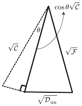
Figure 1: Depict of the triangle relationship (26) between the three real-valued quantities: $\sqrt{\mathcal{F}(\lambda)}$ (3), $\cos\theta(\lambda)\,\sqrt{\mathcal{C}(\lambda)}$ (4), and $\sqrt{\mathcal{D}^{\,}_{\mathrm{un}}(\lambda)}$ (13), where $\theta(\lambda)$ is the Bures angle (5).

IV Reverse triangle inequalities

The discussion presented in the above section indicates that $\mathcal{F}(\lambda)$ is identical to $\cos^{2}\theta(\lambda)\mathcal{C}(\lambda)$ under the exact orthogonality limit (19). This observation motivates us to pursue bounds on the difference between them, namely, $|\sqrt{\mathcal{F}(\lambda)}-\cos^{\,}\theta(\lambda)\sqrt{\mathcal{C}(\lambda)}|$. A useful tool for the present work is the following lemma.

Lemma.

The three real-valued quantities, $\sqrt{\mathcal{F}(\lambda)}$ (3), $\cos\theta(\lambda)\,\sqrt{\mathcal{C}(\lambda)}$ (4), and $\sqrt{\mathcal{D}^{\,}_{\mathrm{un}}(\lambda)}$ (13), obey a set of (reverse) triangle inequalities,

$$|\sqrt{\mathcal{F}(\lambda)}-\cos^{\,}\theta(\lambda)\sqrt{\mathcal{C}(\lambda)}| \leq\sqrt{\mathcal{D}^{\,}_{\mathrm{un}}(\lambda)}.$$ (26a)

$$\left|\sqrt{\mathcal{D}^{\,}_{\mathrm{un}}(\lambda)}-\cos\theta(\lambda)\,\sqrt{\mathcal{C}(\lambda)}\right| \leq\sqrt{\mathcal{F}(\lambda)},$$ (26b)

$$\left|\sqrt{\mathcal{D}^{\,}_{\mathrm{un}}(\lambda)}-\sqrt{\mathcal{F}(\lambda)}\right| \leq\cos\theta(\lambda)\,\sqrt{\mathcal{C}(\lambda)}.$$ (26c)

Thus, $\sqrt{\mathcal{F}(\lambda)}$, $\cos\theta(\lambda)\,\sqrt{\mathcal{C}(\lambda)}$, and $\sqrt{\mathcal{D}^{\,}_{\mathrm{un}}(\lambda)}$, form a triangle on a plane for all values of parameters. See Fig. 1 for an illustration.

Proof.

First, we begin by considering the right side of Eq. (26a) with the help of Eq. (13),

$$\sqrt{\mathcal{D}^{\,}_{\mathrm{un}}(\lambda)} =\Big{|}\langle\Psi^{\,}_{\lambda}|\Phi^{\,}_{\lambda}\rangle-\langle\Psi^{\,}_{\lambda}|\Phi^{\,}_{0}\rangle\langle\Phi^{\,}_{0}|\Phi^{\,}_{\lambda}\rangle\Big{|}$$

$$\geq\Big{|}|\langle\Psi^{\,}_{\lambda}|\Phi^{\,}_{\lambda}\rangle|-|\langle\Psi^{\,}_{\lambda}|\Phi^{\,}_{0}\rangle||\langle\Phi^{\,}_{0}|\Phi^{\,}_{\lambda}\rangle|\Big{|}$$

$$=\Big{|}\sqrt{\mathcal{F}(\lambda)}-\cos\theta(\lambda)\,\sqrt{\mathcal{C}(\lambda)}\Big{|},$$ (27)

where we have used the reverse triangle inequality $|z-w|\geq\left||z|-|w|\right|$ for $z,w\in\mathbb{C}.$ The inequality (26a) is thus established. Note that the right side of Eq. (27) may be interpreted as a lower bound on $\sqrt{\mathcal{D}^{\,}_{\mathrm{un}}(\lambda)}.$

Second, we observe that there is an upper bound on $\sqrt{\mathcal{D}^{\,}_{\mathrm{un}}(\lambda)},$

$$\sqrt{\mathcal{D}^{\,}_{\mathrm{un}}(\lambda)} =\Big{|}\langle\Psi^{\,}_{\lambda}|\Phi^{\,}_{\lambda}\rangle-\langle\Psi^{\,}_{\lambda}|\Phi^{\,}_{0}\rangle\langle\Phi^{\,}_{0}|\Phi^{\,}_{\lambda}\rangle\Big{|}$$

$$\leq|\langle\Psi^{\,}_{\lambda}|\Phi^{\,}_{\lambda}\rangle|+|\langle\Psi^{\,}_{\lambda}|\Phi^{\,}_{0}\rangle||\langle\Phi^{\,}_{0}|\Phi^{\,}_{\lambda}\rangle|$$

$$=\sqrt{\mathcal{F}(\lambda)}+\cos\theta(\lambda)\,\sqrt{\mathcal{C}(\lambda)},$$ (28)

which is a consequence of the triangle inequality, $|z+w|\leq|z|+|w|$ for $z,w\in\mathbb{C}.$

Finally, combing the upper bound (28) with the lower bound (27) yields two two-sided bounds on $\sqrt{\mathcal{D}^{\,}_{\mathrm{un}}(\lambda)}$ (neglecting $\lambda$ to simplify notation),

$$-\sqrt{\mathcal{F}}+\cos\theta\,\sqrt{\mathcal{C}} \leq\sqrt{\mathcal{D}^{\,}_{\mathrm{un}}}\leq\sqrt{\mathcal{F}}+\cos\theta\,\sqrt{\mathcal{C}},$$ (29a)

$$\sqrt{\mathcal{F}}-\cos\theta\,\sqrt{\mathcal{C}} \leq\sqrt{\mathcal{D}^{\,}_{\mathrm{un}}}\leq\sqrt{\mathcal{F}}+\cos\theta\,\sqrt{\mathcal{C}}.$$ (29b)

This completes the proof of Eqs. (26b) and (26c). ∎

The first triangle inequality (26a) provides a quantitative way to understand the closeness between $\mathcal{F}(\lambda)$ and $\mathcal{C}(\lambda)$ since

$$\sqrt{\mathcal{F}}-\sqrt{\mathcal{C}}\;\leq\;\sqrt{\mathcal{F}}-\cos\theta(\lambda)\sqrt{\mathcal{C}}\;\leq\;\sqrt{\mathcal{D}^{\,}_{\mathrm{un}}}.$$ (30)

Since the unnormalized overlap $\sqrt{\mathcal{D}^{\,}_{\mathrm{un}}(\lambda)}$ enters as an upper bound, a small value of $\sqrt{\mathcal{D}^{\,}_{\mathrm{un}}(\lambda)}$, which can be achieved by the two cases of Eq. (22), implies that the numerical difference between the adiabatic fidelity $\mathcal{F}(\lambda)$ and the ground state overlap $\mathcal{C}(\lambda)$ must be small. Note that the set of triangle inequality (26) can also be employed to derive inequality (15) [see SM S1].

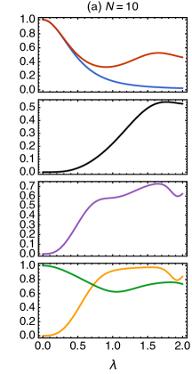
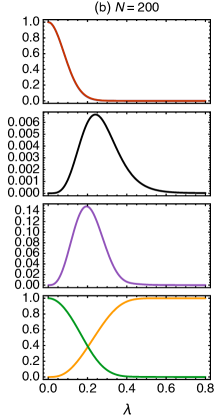
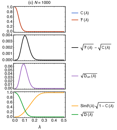
Figure 2: (Color online) Various quantities are calculated numerically for the driven Rice-Mele model (32) with the value of parameters shown in Eq. (36) for system size $N=10,200$ and $1000.$ Further explanation is provided in the main text.

V Illustrative example I: non-interacting Hamiltonians

To demonstrate our general findings, the remaining task is to express $\sqrt{\mathcal{D}^{\,}_{\mathrm{un}}(\lambda)}$ (13) in terms of the Bures angle $\theta(\lambda)$ and the ground state overlap $\mathcal{C}(\lambda)$ explicitly for certain models. This can be done analytically for non-interacting Hamiltonians for which one obtains [see SM S3],

$$\sqrt{\mathcal{D}^{\,}_{\mathrm{un}}(\lambda)}\simeq\cos\theta(\lambda)\sqrt{\mathcal{C}(\lambda)}\left|\sum^{\,}_{k}A^{\,}_{k}\right|,$$ (31a)

$$\text{where}\quad A^{\,}_{k}\,\raisebox{0.85pt}{.}\raisebox{2.85pt}{.}\!\!=\,\frac{\langle\psi^{\,}_{\lambda}(k)|(\mathbb{I}^{\,}_{k}-p^{\,}_{k})|\phi^{\,}_{\lambda}(k)\rangle}{\langle\psi^{\,}_{\lambda}(k)|p^{\,}_{k}|\phi^{\,}_{\lambda}(k)\rangle}.$$ (31b)

where $$|\psi^{\,}_{\lambda}(k)\rangle, |\phi^{\,}_{\lambda}(k)\rangle p^{\,}_{k} |\Psi^{\,}_{\lambda}\rangle, |\Phi^{\,}_{\lambda}\rangle P$$ , and are the single-body counterpart of , and , respectively.

For concreteness, let us consider a time-dependent Rice-Mele model describing a system of fermions on a half-filled one-dimensional bipartite lattice with the Hamiltonian Rice and Mele (1982); Nakajima et al. (2016); Lychkovskiy et al. (2017)

$$H^{\,}_{\mathrm{RM}}\,\raisebox{0.85pt}{.}\raisebox{2.85pt}{.}\!\!=\, \sum^{N}_{j=1}\left[-(J+U)a^{{\dagger}}_{j}b^{\,}_{j}-(J-U)a^{{\dagger}}_{j}b^{\,}_{j+1}+\mathrm{h.c.}\right]$$

$$+\sum^{N}_{j=1}\mu(\lambda)\left(a^{{\dagger}}_{j}a^{\,}_{j}-b^{{\dagger}}_{j}b^{\,}_{j}\right),$$ (32)

where $N$, the number of lattice sites, is assumed to be even. Here, $a^{\,}_{j}$ and $b^{\,}_{j}$ are the fermionic annihilation operators on the $a$ and $b$ sublattices, respectively. For this model with $\mu(\lambda)=\lambda$, the ground state overlap $\mathcal{C}(\lambda)$ (4) and the function $\mathcal{R}(\lambda)$ (8) reads Lychkovskiy et al. (2017),

$$\mathcal{C}(\lambda)=e^{-C^{\,}_{N}\lambda^{2}}\quad\text{and}\quad\mathcal{R}(\lambda)=\frac{\lambda^{2}}{2\Gamma}\delta V^{\,}_{N}$$ (33)

with $C^{\,}_{N}=(16JU)^{-1}N$ and $\delta V^{\,}_{N}=\sqrt{N}.$

We shall specialize to the case where $J=U=$ constant for which the summation in Eq. (31a) can be evaluated in closed form [see SM S3],

$$\sqrt{\mathcal{D}^{\,}_{\mathrm{un}}(\lambda)}\simeq \,\sqrt{\mathcal{C}(\lambda)}\cos\theta(\lambda)\sin\theta(\lambda)\alpha(\lambda),$$ (34a)

$$\sqrt{\mathcal{D}(\lambda)}\simeq \,\sqrt{\mathcal{C}(\lambda)}\cos\theta(\lambda)\alpha(\lambda)/\sqrt{1-\mathcal{C}(\lambda)},$$ (34b)

$$\alpha(\lambda)\,\raisebox{0.85pt}{.}\raisebox{2.85pt}{.}\!\!=\, \,\sqrt{N}\sqrt{1-\mathcal{C}(\lambda)^{1/N}}.$$ (34c)

We now examine whether the explicit form of $\sqrt{\mathcal{D}^{\,}_{\mathrm{un}}(\lambda)}$ (34a) satisfy the two cases of Eq. (22). First, it is readily checked that, for small $\lambda$, the leading order contribution for $\sqrt{\mathcal{D}^{\,}_{\mathrm{un}}(\lambda)}$ (34a) and $\sqrt{\mathcal{D}(\lambda)}$ (34b) are $\mathcal{O}(\lambda^{3})$ and $\mathcal{O}(1)$, respectively, which is consistent with Eq. (25). Second, notice that the function $\alpha(\lambda)$ (34c) scales at most as $\sqrt{N},$

$$\alpha(\lambda)\leq\sqrt{cN\lambda^{2}}=\sqrt{-\ln\mathcal{C}(\lambda)},$$ (35)

as a result of the inequality $1-e^{-x}\leq x$ for all $x\in\mathbb{R}.$ Therefore, we deduce from Eq. (34) that $\sqrt{\mathcal{D}^{\,}_{\mathrm{un}}(\lambda)}\sim\sqrt{\mathcal{D}(\lambda)}\sim\sqrt{\mathcal{C}(\lambda)}\sqrt{N}\to 0$ as $N\to\infty.$ Consequently, the triangle inequality (26a) indicates that $\sqrt{\mathcal{F}(\lambda)}\to\cos^{\,}\theta(\lambda)\sqrt{\mathcal{C}(\lambda)}$ under the same large $N$ limit, as claimed previously in Sec. III.

To numerically demonstrate our findings, we choose the following value of parameters

$$(J,U,\Gamma)=(0.4,0.4,0.7)$$ (36)

in the Hamiltonian $H^{\,}_{\mathrm{RM}}$ (32) as a representative example. In Fig. 2, we plot various quantities for the driven Rice-Mele model (32) with system size $N=10,200$, and $1000.$ In the first row, the adiabatic fidelity $\mathcal{F}(\lambda)$ and the ground state overlap $\mathcal{C}(\lambda)$ are indistinguishable for $N=200$ and $N=1000$. The second row shows that, for both $N=200$ and $N=1000$, the difference between $\sqrt{\mathcal{F}(\lambda)}$ and $\sqrt{\mathcal{C}(\lambda)}$ raises as $\lambda$ increases and then diminishes as $\lambda$ further increases. This bell-shaped curve of $\sqrt{\mathcal{F}(\lambda)}-\sqrt{\mathcal{C}(\lambda)}$ is in phase with the curve of the unnormalized overlap $\sqrt{\mathcal{D^{\,}_{\mathrm{un}}}(\lambda)}$ [third row], which is consistent with the inequality (30). Since $\sqrt{\mathcal{D^{\,}_{\mathrm{un}}}(\lambda)}$ can be factorized into two pieces, c.f. Eq. (14), the smallness of the monotonically increasing part of $\sqrt{\mathcal{F}(\lambda)}-\sqrt{\mathcal{C}(\lambda)}$ is attributed to the smallness of $\sin\theta(\lambda)\sqrt{1-\mathcal{C}(\lambda)}$ [fourth row]. Likewise, the monotonically decreasing part of $\sqrt{\mathcal{F}(\lambda)}-\sqrt{\mathcal{C}(\lambda)}$ is particularly small due to the almost-orthogonality occurring in the complementary space when $N$ is large, which is manifested by a small $\sqrt{\mathcal{D}(\lambda)}$ [fourth row]. By contrast, for $N=10$ [see Fig. 2(a)], $\sqrt{\mathcal{F}(\lambda)}-\sqrt{\mathcal{C}(\lambda)}$ [second row of panel (a)] is monotonically increasing in most of the values of $\lambda$ and is small only in the region of small $\lambda$ (say, $\lambda\leq 0.2$). Again, this smallness of $\sqrt{\mathcal{F}(\lambda)}-\sqrt{\mathcal{C}(\lambda)}$ is related to the smallness of $\sin\theta(\lambda)\sqrt{1-\mathcal{C}(\lambda)}$ [fourth row of panel (a)]. When $\lambda$ further increases, however, the difference between $\sqrt{\mathcal{F}(\lambda)}$ and $\sqrt{\mathcal{C}(\lambda)}$ is notable since the normalized overlap $\sqrt{\mathcal{D}(\lambda)}$ [fourth row of panel (a)] does not exhibit almost-orthogonality for $N=10$.

To further investigate the behavior of the normalized overlap $\sqrt{\mathcal{D}(\lambda)}$, we compare it with the ground state overlap $\sqrt{\mathcal{C}(\lambda)}$ in Fig. 3. Clearly, both $\sqrt{\mathcal{D}(\lambda)}$ [green curve] and $\sqrt{\mathcal{C}(\lambda)}$ [blue curve] decay monotonically with increasing $N$ and $\lambda$. Besides, notice that $\sqrt{\mathcal{D}(\lambda)}$ decays slower than $\sqrt{\mathcal{C}(\lambda)}$ does. As for a comparison, the unnormalized overlap $\sqrt{\mathcal{D}^{\,}_{\mathrm{un}}(\lambda)}$ [purple curve] is also plotted in Fig. 3.

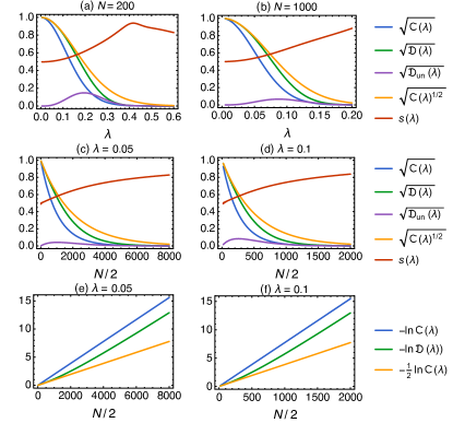
Figure 3: (Color online) Various quantities, $\sqrt{\mathcal{C}(\lambda)}$ (4), $\sqrt{\mathcal{D}(\lambda)}$ (12), $\sqrt{\mathcal{D}^{\,}_{\mathrm{un}}(\lambda)}$ (13), $\sqrt{\mathcal{C}(\lambda)^{1/2}}$, and $s(\lambda)$ (38) for the driven Rice-Mele model (32) are plotted as a function of $\lambda$ or $N$.

Given the explicit form of $\sqrt{\mathcal{D}^{\,}_{\mathrm{un}}(\lambda)}$ (34a), we may substitute it into Eq. (15) and apply the quantum speed limit (6) to obtain the following inequality

$$\left|\mathcal{F}(\lambda)-\mathcal{C}(\lambda)\right|\,\leq\,g(\lambda),\quad g(\lambda)\,\raisebox{0.85pt}{.}\raisebox{2.85pt}{.}\!\!=\,g^{\,}_{1}(\lambda)+g^{\,}_{2}(\lambda),$$ (37a)

$$g^{\,}_{1}(\lambda)\,\raisebox{0.85pt}{.}\raisebox{2.85pt}{.}\!\!=\,\sin^{2}\widetilde{\mathcal{R}}(\lambda)\mathcal{C}(\lambda)\left|-1+\alpha(\lambda)^{2}\right|,$$ (37b)

$$g^{\,}_{2}(\lambda)\,\raisebox{0.85pt}{.}\raisebox{2.85pt}{.}\!\!=\,\sin\Big{(}2\widetilde{\widetilde{\mathcal{R}}}(\lambda)\Big{)}\,\mathcal{C}(\lambda)\alpha(\lambda),$$ (37c)

where $\widetilde{\mathcal{R}}(\lambda)$ and $\widetilde{\widetilde{\mathcal{R}}}(\lambda)$ are defined in Eq. (6) and Eq. (18d), respectively. Note that combing the inequality (37) with the defining range of $\mathcal{F}(\lambda),$ i.e., $\mathcal{F}(\lambda)\in[0,1]$, yields the following two-sided bound on the adiabatic fidelity $\mathcal{F}(\lambda)$

$$\max\left(\mathcal{C}(\lambda)-g(\lambda),0\right)\leq\mathcal{F}(\lambda)\leq\min\left(\mathcal{C}(\lambda)+g(\lambda),1\right),$$

which provides a way to estimate the adiabatic fidelity $\mathcal{F}(\lambda)$ in terms of the ground state overlap $\mathcal{C}(\lambda)$ (4) and the function $\mathcal{R}(\lambda)$ (6b).

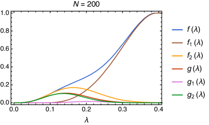
Figure 4: (Color online) Compare the behavior of the function $g(\lambda)=g^{\,}_{1}(\lambda)+g^{\,}_{2}(\lambda)$ (37) with the function $f(\lambda)=f^{\,}_{1}(\lambda)+f^{\,}_{2}(\lambda)$ (18) for $N=200.$

In Fig. 4, we compare an upper bound on $|\mathcal{F}(\lambda)-\mathcal{C}(\lambda)|$ from $g(\lambda)=g^{\,}_{1}(\lambda)+g^{\,}_{2}(\lambda)$ (37) with that from $f(\lambda)=f^{\,}_{1}(\lambda)+f^{\,}_{2}(\lambda)$ (18). The result shows that the function $f(\lambda)$ [blue curve] is monotonically increasing in $\lambda$, whereas the function $g(\lambda)$ [red curve] has a bell-shape. Thus, the function $g(\lambda)$ behaves better than the function $f(\lambda)$ as an upper bound. The improvement of $g(\lambda)$ at large $\lambda$ is attributed to the function $g^{\,}_{1}(\lambda)$ (37b) in which an exponentially decaying factor $\mathcal{C}(\lambda)$ is factorized out [compare to $f^{\,}_{1}(\lambda)$ (18b)]. In the meantime, the function $g^{\,}_{2}(\lambda)$ [green curve], compared to $f^{\,}_{2}(\lambda)$ [orange curve], does not change dramatically. Consequently, among the two inequalities, Eq. (18) and Eq. (37), the inequality (37) serves as a better estimate on the adiabatic fidelity $\mathcal{F}(\lambda).$ We present in Fig. 5 a comparison of estimates on the adiabatic fidelity $\mathcal{F}(\lambda)$ using the inequality (18) [blue-shaded region] and the improved inequality (37) [red-shaded region]. A significant improvement in estimation is achieved using Eq. (37).

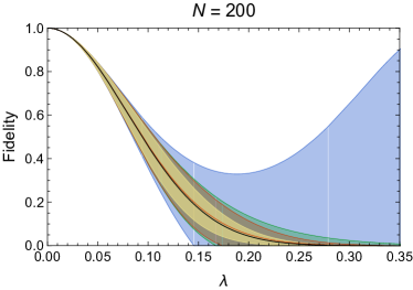
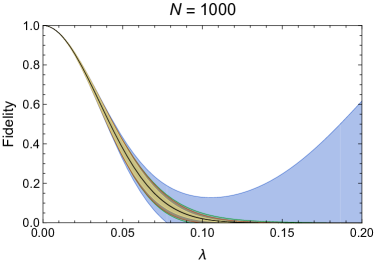
Figure 5: (Color online) Bounds on the adiabatic fidelity $\mathcal{F}(\lambda)$ for $N=200$ and $N=1000$ using Eq. (18) [blue-shaded region], Eq. (37) [red-shaded region], and Eq. (39) with $s=1/2$ [green-shaded region] and $s=1$ [yellow-shaded region]. For both figures, the actual adiabatic fidelity $\mathcal{F}(\lambda)$ is the black curve, while the red curve is for the ground state overlap $\mathcal{C}(\lambda)$, which is, however, not distinct from $\mathcal{F}(\lambda)$.

VI Asymptotic form of the overlap $\mathcal{D}(\lambda)$ and implications

While the function $g(\lambda)$ (37), compared to the function $f(\lambda)$ (18), serves as a better upper bound on $|\mathcal{F}(\lambda)-\mathcal{C}(\lambda)|$; for generic many-body systems, it could be difficult to calculate the overlap $\mathcal{D}(\lambda)$ explicitly, which is essential for the improvement in $g(\lambda)$. We thus seek for a universal scaling form of $\mathcal{D}(\lambda)$, upon which an estimate of upper bound on $|\mathcal{F}(\lambda)-\mathcal{C}(\lambda)|$ can be obtained by means of Eq. (15) without calculating $\mathcal{D}(\lambda)$ from scratch. In light of the reasoning of almost-orthogonality presented in Sec. III.2, we consider the following ratio

$$s(\lambda)\,\raisebox{0.85pt}{.}\raisebox{2.85pt}{.}\!\!=\,\frac{\ln\mathcal{D}(\lambda)}{\ln\mathcal{C}(\lambda)}.$$ (38)

The value of $s(\lambda)\geq 0$ indicates how fast the overlap $\mathcal{D}(\lambda)$ decays compared to the overlap $\mathcal{C}(\lambda).$ If the ratio $s(\lambda)$ takes values in $[0,1]$, then the overlap $\mathcal{D}(\lambda)$ decays not faster than the overlap $\mathcal{C}(\lambda)$ does.

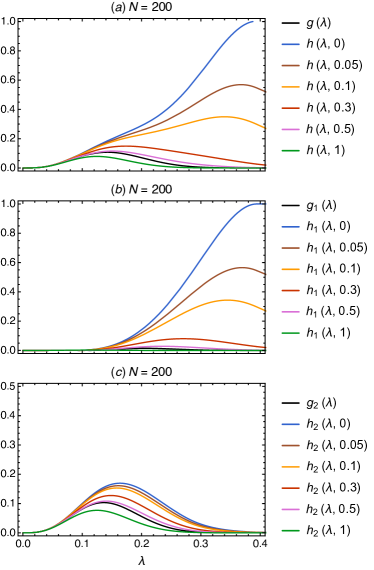
Figure 6: (Color online) Compare the behavior of the function $h^{\,}(\lambda,s)$ (39), $h^{\,}_{1}(\lambda,s)$ (39), and $h^{\,}_{2}(\lambda,s)$ (39) with different constant values of $s.$ As for a comparison, the function $g(\lambda)=g^{\,}_{1}(\lambda)+g^{\,}_{2}(\lambda)$ (37) is also depicted.

Substituting $\mathcal{D}(\lambda)$ using Eq. (38), namely, $\mathcal{D}(\lambda)=\left(\mathcal{C}(\lambda)\right)^{s}$, into Eq. (15) and then applying the inequality of quantum speed limit (6) yields the following inequality,

$$\left|\mathcal{F}(\lambda)-\mathcal{C}(\lambda)\right|\,\leq\,h(\lambda,s)\equiv h^{\,}_{1}(\lambda,s)+h^{\,}_{2}(\lambda,s),$$

$$h^{\,}_{1}(\lambda,s)\,\raisebox{0.85pt}{.}\raisebox{2.85pt}{.}\!\!=\,\sin^{2}\widetilde{\mathcal{R}}(\lambda)\mathcal{C}(\lambda)\left|-1+\mathcal{C}(\lambda)^{s-1}-\mathcal{C}(\lambda)^{s}\right|,$$

$$h^{\,}_{2}(\lambda,s)\,\raisebox{0.85pt}{.}\raisebox{2.85pt}{.}\!\!=\,\sin\Big{(}2\widetilde{\widetilde{\mathcal{R}}}(\lambda)\Big{)}\sqrt{\mathcal{C}(\lambda)^{s+1}}\sqrt{1-\mathcal{C}(\lambda)},$$ (39)

where $\widetilde{\mathcal{R}}(\lambda)$ and $\widetilde{\widetilde{\mathcal{R}}}(\lambda)$ are defined in Eqs. (6a) and (18d), respectively. The inequality (39) should be compared with that of Eq. (18), Eq. (21), and Eq. (37). Note that if $s=0$, then the function $h(\lambda,s=0)$ reduces to the function $f(\lambda)$ of Eq. (18). Observe that the function $h(\lambda,s)$ of Eq. (39) may be read as $\sin\mathcal{R}(\lambda)\mathcal{C}(\lambda)\times(\cdots)$ with the terms in the parenthesis scale at most polynomially in $N$ and $\lambda$ for $s$ not too small; what dominates asymptotically for large $N$ and $\lambda$ in the function $h(\lambda,s)$ is the $\sin\mathcal{R}(\lambda)\mathcal{C}(\lambda)$ factor. This is also the case for Eq. (21) and for the function $g(\lambda)$ of Eq. (37), but it is not the case for the function $f(\lambda)$ of Eq. (18). In other words, only the large $\lambda$ behavior of the function $h^{\,}_{1}(\lambda,s)$ determines whether the function $h^{\,}(\lambda,s)$ can serve as a good upper bound. While generically the exponent $s$ (38) is a function of both $\lambda$ and $N$, we can search for certain limits of $s$ that are a constant in both $\lambda$ and $N$ with which one may obtain general features of an improved upper bound on $|\mathcal{F}(\lambda)-\mathcal{C}(\lambda)|$ using Eq. (39).

Consider again the driven Rice-Mele model presented in Sec. V. In Fig. 6, we plot $h^{\,}(\lambda,s)=h^{\,}_{1}(\lambda,s)+h^{\,}_{2}(\lambda,s)$ (39) as a function of $\lambda$ for different constant values of $s$. We see that as long as $s$ is not too small, $h^{\,}_{1}(\lambda,s)$ [see Fig. 6(b)] decays quickly at large $\lambda$, which improves the tail behavior of the function $h^{\,}(\lambda,s)$ [see Fig. 6(a)]. Observe that the behavior of $h^{\,}_{2}(\lambda,s)$ [see Fig. 6(c)] does not change significantly as $s$ varies. Nevertheless, as long as the exponent $s$ is sufficiently large, the function $h^{\,}(\lambda,s)$ is dominated by $h^{\,}_{2}(\lambda,s)$ and serves as a strong upper bound on $|\mathcal{F}(\lambda)-\mathcal{C}(\lambda)|$. In Fig. 5, we plot bounds on the adiabatic fidelity $\mathcal{F}(\lambda)$ for $N=200$ and $N=1000$ using Eq. (39) with $s=1/2$ [green-shaded region] and $s=1$ [yellow-shaded region]. Note that the case of $s=0$ reduces to the inequality (18) [blue-shaded region] obtained by us previously in Ref. Chen and Cheianov (2022). Observe that the difference between the green-shaded area and the red-shaded area is not significant. That is to say, the result of taking $s=1/2$, namely, taking $\mathcal{D}(\lambda)\approx\sqrt{\mathcal{C}(\lambda)}$, is very close to the result obtained from the inequality (37), which is derived using an explicit form of the unnormalized overlap $\mathcal{D}(\lambda)$ (34b). Consequently, we also plot $\sqrt{\mathcal{C}(\lambda)}$ and $s(\lambda)$ (38) in Fig. 3, which shows that $\sqrt{\mathcal{C}(\lambda)}$ is slightly larger than $\mathcal{D}(\lambda)$. Nevertheless, for the purpose of estimating the adiabatic fidelity $\mathcal{F}(\lambda)$ using the inequality (39), replacing $s(\lambda)$ by a constant value (such as $1/2$)$\sqrt{\mathcal{C}(\lambda)}$ may be a good approximation.

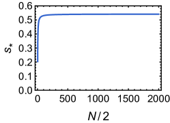
Figure 7: (Color online) The exponent $s^{\,}_{*}$, defined in Eq. (38) with $\lambda=\lambda^{\,}_{*}$ (so that $\mathcal{C}(\lambda^{\,}_{*})=1/e$), is calculated numerically for the driven Rice-Mele model (32) with the value of parameters shown in Eq. (36). Asymptotically, $s^{\,}_{*}=\mathcal{O}(1)$ as $N\to\infty.$

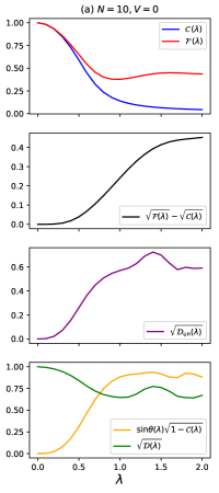
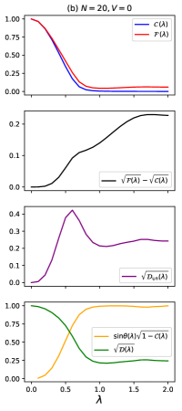
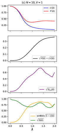
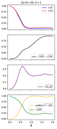
Figure 8: (Color online) Various quantities are calculated numerically for the driven interacting Kitaev chain model (42) with the value of parameters shown in Eq. (43) for system size $N=10$ and $20$ with interaction strength $V=0$ and $V=1.$ Further explanation is provided in the main text.

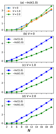
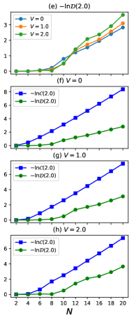
Figure 9: (Color online) The quantities $-\ln\mathcal{C}(\lambda)$ (4) and $-\ln\mathcal{D}(\lambda)$ (12) for the driven interacting Kitaev model (42) are plotted as a function of $N$ for different values of $\lambda$ ($\lambda=1$ in the left column and $\lambda=2$ in the right column) and $V=0,1,2$.

Before concluding this section, let us discuss an implication on a condition for adiabaticity breakdown using inequality (30). Recall that there is a large class of driven many-body systems in which the following condition holds Lychkovskiy et al. (2017)

$$\delta V^{\,}_{N}/C^{\,}_{N}=0\quad\text{as}\quad N\to\infty,$$ (40)

where $\delta V^{\,}_{N}$ is introduced in Eq. (8) and $C^{\,}_{N}$ is the exponent defined through $C(\lambda)=e^{-C^{\,}_{N}\lambda^{2}}$ as $N\to\infty.$ Define $\lambda^{\,}_{*}$ as an adiabatic mean free path so that $\mathcal{F}(\lambda)\geq e^{-1}$ for $\lambda\leq\lambda^{\,}_{*}.$ Here, $\lambda^{\,}_{*}$ is determined by $\mathcal{C}(\lambda^{\,}_{*})=1/e$. The relation $\mathcal{R}(\lambda^{\,}_{*})=\delta V^{\,}_{N}/(2\Gamma C^{\,}_{N})$ then follows from Eq. (8). It was shown in Ref. Lychkovskiy et al. (2017) that, in order to avoid adiabaticity breakdown, the driving rate $\Gamma$ of driven many-body systems must scale down with increasing system size $N$. With inequality (30), we find that quantum adiabaticity is maintained if $\Gamma\leq\Gamma^{\,}_{N}$ where [see SM S4 for a derivation]

$$\Gamma^{\,}_{N}\,\raisebox{0.85pt}{.}\raisebox{2.85pt}{.}\!\!=\,\frac{1}{2}\frac{\delta V^{\,}_{N}}{C^{\,}_{N}}\frac{1}{\left(1-\epsilon-e^{-1/2}\right)^{2}}M(s^{\,}_{*})$$ (41)

with $\epsilon\in[0,1]$, $M(s^{\,}_{*})\,\raisebox{0.85pt}{.}\raisebox{2.85pt}{.}\!\!=\,\sqrt{1-e^{-1}}\,e^{-s^{\,}_{*}/2}$ and $s^{\,}_{*}\,\raisebox{0.85pt}{.}\raisebox{2.85pt}{.}\!\!=\,s(\lambda^{\,}_{*})=-\ln\mathcal{D}(\lambda^{\,}_{*})$. Therefore, the asymptotic form of $M(s^{\,}_{*})$ as $N\to\infty$ contributes to a multiplicative modification to the scaling form $\Gamma^{\,}_{N}\sim\delta V^{\,}_{N}/C^{\,}_{N}$ found previously in Refs. Lychkovskiy et al. (2017); Chen and Cheianov (2022). If $s^{\,}_{*}=\mathcal{O}(1)$ as $N\to\infty$, then $M(s^{\,}_{*})=\mathcal{O}(1)$; while if $s^{\,}_{*}=\mathcal{O}(N^{c})$ with $c\in\mathbb{R}$ as $N\to\infty,$ then $M(s^{\,}_{*})=\mathcal{O}(e^{-N^{c}}).$ One verifies that if the leading asymptotics of $-\ln\mathcal{D}(\lambda)$ is proportional to that of $-\ln\mathcal{C}(\lambda)=C^{\,}_{N}\lambda^{2}$ as $N\to\infty,$ then $s^{\,}_{*}=\mathcal{O}(1)$ holds. For the driven Rice-Mele model (32), we find $s^{\,}_{*}=\mathcal{O}(1)$ as $N\to\infty$ [see Fig. 7], renders $M(s^{\,}_{*})=\mathcal{O}(1)$.

VII Illustrative example II: interacting fermions

Thus far, our general results have been illustrated using the driven Rice-Mele model (32), a model of quadratic fermions with the property that the underlying Hilbert space can be constructed as a direct product of single-particle states. A fascinating question arises regarding whether the statement of almost-orthogonality between vectors in the complement of the initial state continues to hold for typical many-body systems, specifically those controlled by nonintegrable interacting Hamiltonians. In order to investigate this question, we examine an interacting Kitaev chain model described by the following Hamiltonian,

$$H^{\,}_{\mathrm{K}}\,\raisebox{0.85pt}{.}\raisebox{2.85pt}{.}\!\!=\, \sum^{N}_{j=1}\left[\left(-Jc^{{\dagger}}_{j}c^{\,}_{j+1}+\Delta c^{{\dagger}}_{j}c^{{\dagger}}_{j+1}+\mathrm{h.c.}\right)+Vn^{\,}_{j}n^{\,}_{j+1}\right]$$

$$+\sum^{N}_{j=1}\mu(\lambda)n^{\,}_{j},$$ (42)

where $n^{\,}_{j}\,\raisebox{0.85pt}{.}\raisebox{2.85pt}{.}\!\!=\,c^{{\dagger}}_{j}c^{\,}_{j}$ is the number operator of fermions at lattice site $j$, $N$ the number of lattice sites, $J$ the hopping amplitude, $\Delta$ the superconducting pairing amplitude, $V$ the strength of nearest-neighbor Coulomb repulsion, and $\mu(\lambda)=\mu^{\,}_{0}\lambda$ (with $\mu^{\,}_{0}\in\mathbb{R}$) the time-dependent chemical potential. If $V=0,$ the Hamiltonian (42) reduces to that of the Kitaev model of one-dimensional $p$-wave superconductors Kitaev (2001). We shall consider the Hamiltonian (42) with periodic boundary conditions and the sector of odd fermion parity. To ensure the numerical simulation results reflect generic features, we avoid selecting parameter values that correspond to solvable points Chepiga and Mila (2023). For concreteness, we choose the following value of parameters

$$(J,\Delta,\mu^{\,}_{0},\Gamma)=(1.0,0.8,3.0,1.0).$$ (43)

In Fig. 8, we plot various quantities as a function of $\lambda$ for the driven interacting Kitaev model (42) for system size $N=10$ [in panels (a) and (c)] and $N=20$ [in panels (b) and (d)] with interaction strength $V=0$ [in panels (a) and (b)] and $V=1$ [in panels (c) and (d)]. Panel (a) and panel (b) represent the case of driven non-interacting Kitaev model for system size $N=10$ and $N=20,$ respectively. Observe that the behavior of various curves in panel (a) is quantitatively similar to those of driven Rice-Mele model with $N=10$ presented in Fig. 2(a). When we increase the system size to $N=20,$ which is close to the limit of computational ability set by the exact diagonalization method, the main feature is a faster decay of $\mathcal{F}(\lambda)$, $\mathcal{C}(\lambda),$ and $\mathcal{D}(\lambda),$ as shown in Fig. 8(b). This finding agrees with the observations made for the driven Rice-Mele model presented in Fig. 2. Figure 8(c) and Fig. 8(d) represent the case of driven interacting Kitaev model with $V=1$ for system size $N=10$ and $N=20,$ respectively. Compared with the non-interacting counterpart, differences between panel (c) and panel (a) or between panel (d) and panel (b) are not significant. Therefore, we anticipate that the phenomena of almost-orthogonality between vectors in the complement of the initial state should persist even in the presence of interacting Hamiltonians. To further elucidate this point, we plot in Fig. 9 the quantities $-\ln\mathcal{C}(\lambda)$ (4) and $-\ln\mathcal{D}(\lambda)$ (12) for the driven interacting Kitaev model (42) as a function of system size $N$ for $\lambda=1,2$ and interaction strength $V=0,1,2$. According to all the panels of Fig. 9, the normalized overlap $\mathcal{D}(\lambda)$ decays with increasing system size $N$, a characteristic of almost-orthogonality in complementary subspace. Before concluding this section, note that there are two other interesting numerical observations. First, the ground state overlap $\mathcal{C}(\lambda)$ decays faster than the normalized overlap $\mathcal{D}(\lambda)$, a feature found similarly in the driven Rice-Mele model (recall Fig. 3). Second, the decay rate of $\mathcal{D}(\lambda)$ increases with increasing interaction strength $V$.

VIII Summary and Outlook

An explanation has been given in this study as to why in quantum many-body systems, the adiabatic fidelity, $\mathcal{F}(\lambda),$ and the overlap between the initial state and instantaneous ground states, $\mathcal{C}(\lambda),$ have nearly identical values in many cases. While in the region of small evolution parameter $\lambda$ the question can be addressed by an explicit calculation from perturbation theory, which shows that the difference between $\mathcal{F}(\lambda)$ and $\mathcal{C}(\lambda)$ only appears at order $\lambda^{3}$; a satisfactory answer to the question relies on an inherent property of quantum many-body systems, namely, almost-orthogonality of random vectors. Specifically, we have discussed in detail how the almost-orthogonality occurring in the complementary space of the initial state, as exhibited by an exponentially decaying normalized overlap $\mathcal{D}(\lambda)$ (12) and a small value of unnormalized overlap $\mathcal{D}^{\,}_{\mathrm{un}}(\lambda)$ (13), controls an upper bound [see Eq. (30)] on the difference between $\sqrt{\mathcal{F}(\lambda)}$ and $\sqrt{\mathcal{C}(\lambda)}$ [or between $\mathcal{F}(\lambda)$ and $\mathcal{C}(\lambda)$]. Our study further provides improved estimates on the adiabatic fidelity $\mathcal{F}(\lambda)$ based on an explicit form of the normalized overlap $\mathcal{D}(\lambda)$ expressed in terms of certain functions of the ground state overlap $\mathcal{C}(\lambda).$ These estimates on the adiabatic fidelity $\mathcal{F}(\lambda)$ have been illustrated using the driven Rice-Mele model and shown to perform well even for system size $N=\mathcal{O}(10^{2})$, which is the same large $N$ limit for which the ground state overlap $\mathcal{C}(\lambda)$ can be accurately approximated by a form of generalized orthogonality catastrophe, i.e., $\mathcal{C}(\lambda)\approx e^{-C^{\,}_{N}\lambda^{2}}.$ It is noteworthy that previous estimates on the adiabatic fidelity $\mathcal{F}(\lambda)$ obtained by Ref. Lychkovskiy et al. (2017) and Ref. Chen and Cheianov (2022) only work well for system size $N=\mathcal{O}(10^{4})$ and $N=\mathcal{O}(10^{3}),$ respectively.

We conclude by mentioning that it would be worthwhile to pursue rigorous proof, on par with Ref. Gebert et al. (2014), to establish the existence of subspace almost-orthogonality. Moreover, it would also be intriguing to investigate the potential significance of subspace almost-orthogonality in alternative settings of driven many-body systems that are know to exhibit orthogonality catastrophe in the full Hilbert space, including systems of time-dependent impurity Knap et al. (2012) and quantum quench Schiró and Mitra (2014).

Acknowledgments. The numerical calculations of Sec. VII were accomplished using QuSpin Weinberg and Bukov (2017, 2019). This work is part of the Adiabatic Protocols in Extended Quantum Systems project, funded by the Dutch Research Council (NWO) under Project No 680-91-130.

S1 Derivation of Eq. (15)

We want to derive the inequality (15), which is first derived in Ref. Chen and Cheianov (2022), using a more compact notation. First, we compute $\mathcal{F}(\lambda)$ using Eq. (9a),

$$\mathcal{F}(\lambda) =|\langle\Phi^{\,}_{\lambda}|(P+Q)|\Psi^{\,}_{\lambda}\rangle|^{2}$$

$$=|\langle\Phi^{\,}_{\lambda}|P|\Psi^{\,}_{\lambda}\rangle+\langle\Phi^{\,}_{\lambda}|Q|\Psi^{\,}_{\lambda}\rangle|^{2}$$

$$=|\langle\Phi^{\,}_{\lambda}|P|\Psi^{\,}_{\lambda}\rangle|^{2}+|\langle\Phi^{\,}_{\lambda}|Q|\Psi^{\,}_{\lambda}\rangle|^{2}+2\Re\Big{(}\langle\Psi^{\,}_{\lambda}|P|\Phi^{\,}_{\lambda}\rangle\langle\Phi^{\,}_{\lambda}|Q|\Psi^{\,}_{\lambda}\rangle\Big{)}.$$ (S1)

Combing (i) Eq. (S1), (ii) the triangle inequality for absolute value, (iii) the inequality $\Re(z)\leq|z|$ for $z\in\mathbb{C}$, and (iv) Eqs.  (10) and (12) yields the following chain of inequalities

$$\left|\mathcal{F}(\lambda)-\mathcal{C}(\lambda)\right|\stackrel{{\scriptstyle\rm(i)}}{{=}} \,\Bigg{|}|\langle\Phi^{\,}_{\lambda}|P|\Psi^{\,}_{\lambda}\rangle|^{2}-\mathcal{C}(\lambda)+|\langle\Phi^{\,}_{\lambda}|Q|\Psi^{\,}_{\lambda}\rangle|^{2}+2\Re\Big{(}\langle\Psi^{\,}_{\lambda}|P|\Phi^{\,}_{\lambda}\rangle\langle\Phi^{\,}_{\lambda}|Q|\Psi^{\,}_{\lambda}\rangle\Big{)}\Bigg{|}$$

$$\stackrel{{\scriptstyle\rm(ii)}}{{\leq}} \,\Bigg{|}|\langle\Phi^{\,}_{\lambda}|P|\Psi^{\,}_{\lambda}\rangle|^{2}-\mathcal{C}(\lambda)+|\langle\Phi^{\,}_{\lambda}|Q|\Psi^{\,}_{\lambda}\rangle|^{2}\Bigg{|}+2\Bigg{|}\Re\Big{(}\langle\Psi^{\,}_{\lambda}|P|\Phi^{\,}_{\lambda}\rangle\langle\Phi^{\,}_{\lambda}|Q|\Psi^{\,}_{\lambda}\rangle\Big{)}\Bigg{|}$$

$$\stackrel{{\scriptstyle\rm(iii)}}{{\leq}} \,\Bigg{|}|\langle\Phi^{\,}_{\lambda}|P|\Psi^{\,}_{\lambda}\rangle|^{2}-\mathcal{C}(\lambda)+|\langle\Phi^{\,}_{\lambda}|Q|\Psi^{\,}_{\lambda}\rangle|^{2}\Bigg{|}+2\left|\langle\Psi^{\,}_{\lambda}|P|\Phi^{\,}_{\lambda}\rangle\right|\left|\langle\Phi^{\,}_{\lambda}|Q|\Psi^{\,}_{\lambda}\rangle\right|$$

$$\stackrel{{\scriptstyle\rm(iv)}}{{=}} \,\left|-\sin^{2}\theta(\lambda)\mathcal{C}(\lambda)+\mathcal{D}^{\,}_{\mathrm{un}}(\lambda)\right|+2\cos\theta(\lambda)\sqrt{\mathcal{C}(\lambda)}\sqrt{\mathcal{D}^{\,}_{\mathrm{un}}(\lambda)}.$$ (S2)

Alternative derivation

Alternatively, the inequality (15) can also be obtained using the set of triangle inequality (26). We begin with the upper bound on $\sqrt{\mathcal{F}(\lambda)}$ from Eq. (26a), $\sqrt{\mathcal{F}(\lambda)}\leq\cos^{\,}\theta(\lambda)\sqrt{\mathcal{C}(\lambda)}+\sqrt{\mathcal{D}^{\,}_{\mathrm{un}}(\lambda)}$, and then calculate $\mathcal{F}(\lambda)-\mathcal{C}(\lambda)$,

$$\mathcal{F}(\lambda)-\mathcal{C}(\lambda) \quad\leq\quad-\sin^{2}\theta(\lambda)\mathcal{C}(\lambda)+\mathcal{D}^{\,}_{\mathrm{un}}(\lambda)+2\cos^{\,}\theta(\lambda)\sqrt{\mathcal{C}(\lambda)}\sqrt{\mathcal{D}^{\,}_{\mathrm{un}}(\lambda)}$$

$$\quad\leq\quad\left|-\sin^{2}\theta(\lambda)\mathcal{C}(\lambda)+\mathcal{D}^{\,}_{\mathrm{un}}(\lambda)\right|+2\cos^{\,}\theta(\lambda)\sqrt{\mathcal{C}(\lambda)}\sqrt{\mathcal{D}^{\,}_{\mathrm{un}}(\lambda)},$$ (S3)

where the last step is obtained after using the inequality, $x+y\leq|x+y|$ for $x,y\in\mathbb{R}.$ Similarly, we consider the lower bound on $\sqrt{\mathcal{F}(\lambda)}$ from Eq. (26b), $\sqrt{\mathcal{F}(\lambda)}\geq\left|\sqrt{\mathcal{D}^{\,}_{\mathrm{un}}(\lambda)}-\cos\theta(\lambda)\,\sqrt{\mathcal{C}(\lambda)}\right|$, and then calculate $\mathcal{F}(\lambda)-\mathcal{C}(\lambda)$,

$$\mathcal{F}(\lambda)-\mathcal{C}(\lambda) \quad\geq\quad-\sin^{2}\theta(\lambda)\mathcal{C}(\lambda)+\mathcal{D}^{\,}_{\mathrm{un}}(\lambda)-2\cos^{\,}\theta(\lambda)\sqrt{\mathcal{C}(\lambda)}\sqrt{\mathcal{D}^{\,}_{\mathrm{un}}(\lambda)}$$

$$\quad\geq\quad-\left|-\sin^{2}\theta(\lambda)\mathcal{C}(\lambda)+\mathcal{D}^{\,}_{\mathrm{un}}(\lambda)\right|-2\cos^{\,}\theta(\lambda)\sqrt{\mathcal{C}(\lambda)}\sqrt{\mathcal{D}^{\,}_{\mathrm{un}}(\lambda)},$$ (S4)

where the last step is obtained after using the inequality, $x+y\geq-|x+y|$ for $x,y\in\mathbb{R}.$ Combing Eqs. (S3) with (S4) yields the inequality (15).

S2 Perturbative expansion in $\lambda$

A detailed derivation of Eqs. (24) and (25) is provided.

S2.1 For instantaneous ground state

We want to solve the instantaneous eigenvalue equation (2) perturbatively in $\lambda$,

$$H^{\,}_{\lambda}|\Phi^{\,}_{\lambda}\rangle=E^{\,}_{\mathrm{GS},\lambda}|\Phi^{\,}_{\lambda}\rangle,\quad H^{\,}_{\lambda}=H^{\,}_{0}+\lambda V,$$ (S5)

given $H^{\,}_{0}|\chi^{\,}_{n}\rangle=\varepsilon^{\,}_{n}|\chi^{\,}_{n}\rangle,$ where $|\Phi^{\,}_{\lambda}\rangle$ is the ground state of $H^{\,}_{\lambda},$ and $\{|\chi^{\,}_{n}\rangle\}$ is a set of the complete orthonormal eigenstates of $H^{\,}_{0}$ with $|\chi^{\,}_{0}\rangle\equiv|\Psi^{\,}_{0}\rangle$ being the ground state of $H^{\,}_{0}$ and $n=0,1,\cdots$ labels distinct eigenstates. Apply the standard Rayleigh-Schrödinger perturbation theory up to order $\lambda^{2}$ yields the following series,

$$|\Phi^{\,}_{\lambda}\rangle= \,\left(1-\frac{\lambda^{2}}{2}\sum^{\,}_{n\neq 0}\frac{|V^{\,}_{n0}|^{2}}{(\varepsilon^{\,}_{0}-\varepsilon^{\,}_{n})^{2}}\right)|\chi^{\,}_{0}\rangle+\lambda\sum^{\,}_{n\neq 0}\frac{V^{\,}_{n0}}{\varepsilon^{\,}_{0}-\varepsilon^{\,}_{n}}\,|\chi^{\,}_{n}\rangle+\lambda^{2}\sum^{\,}_{n\neq 0}\frac{1}{\varepsilon^{\,}_{0}-\varepsilon^{\,}_{n}}\left(\sum^{\,}_{m\neq 0}\frac{V^{\,}_{nm}V^{\,}_{m0}}{\varepsilon^{\,}_{0}-\varepsilon^{\,}_{m}}-\frac{V^{\,}_{00}V^{\,}_{n0}}{\varepsilon^{\,}_{0}-\varepsilon^{\,}_{n}}\right)|\chi^{\,}_{n}\rangle+\cdots,$$ (S6)

where $V^{\,}_{nm}\,\raisebox{0.85pt}{.}\raisebox{2.85pt}{.}\!\!=\,\langle\chi^{\,}_{n}|V|\chi^{\,}_{m}\rangle.$ Hence, the following inner products are obtained,

$$\langle\chi^{\,}_{0}|\Phi^{\,}_{\lambda}\rangle=1-\frac{\lambda^{2}}{2}\sum^{\,}_{n\neq 0}\frac{|V^{\,}_{n0}|^{2}}{(\varepsilon^{\,}_{0}-\varepsilon^{\,}_{n})^{2}}+\lambda^{3}\Bigg{(}\sum^{\,}_{n\neq 0}\frac{V^{\,}_{00}|V^{\,}_{n0}|^{2}}{(\varepsilon^{\,}_{0}-\varepsilon^{\,}_{n})^{3}}-\sum^{\,}_{n\neq 0}\frac{1}{(\varepsilon^{\,}_{0}-\varepsilon^{\,}_{n})^{2}}\sum^{\,}_{m\neq 0}\frac{\Re(V^{*}_{nm}V^{*}_{m0}V^{\,}_{n0})}{\varepsilon^{\,}_{0}-\varepsilon^{\,}_{m}}\Bigg{)}+\cdots.$$ (S7a)

$$\langle\chi^{\,}_{n\neq 0}|\Phi^{\,}_{\lambda}\rangle=\lambda\frac{V^{\,}_{n0}}{\varepsilon^{\,}_{0}-\varepsilon^{\,}_{n}}+\lambda^{2}\frac{1}{\varepsilon^{\,}_{0}-\varepsilon^{\,}_{n}}\left(\sum^{\,}_{m\neq 0}\frac{V^{\,}_{nm}V^{\,}_{m0}}{\varepsilon^{\,}_{0}-\varepsilon^{\,}_{m}}-\frac{V^{\,}_{00}V^{\,}_{n0}}{\varepsilon^{\,}_{0}-\varepsilon^{\,}_{n}}\right)+\cdots.$$ (S7b)

Notice that both inner products, $\langle\chi^{\,}_{0}|\Phi^{\,}_{\lambda}\rangle$ and $\langle\chi^{\,}_{n\neq 0}|\Phi^{\,}_{\lambda}\rangle$, are real-valued.

S2.2 For time-evolved state

We want to solve the time-dependent Schrödinger equation (1) perturbatively,

$$\mathrm{i}\Gamma\partial^{\,}_{\lambda}|\Psi^{\,}_{\lambda}\rangle=\left(H^{\,}_{0}+\lambda V\right)|\Psi^{\,}_{\lambda}\rangle,\quad|\Psi^{\,}_{0}\rangle=|\chi^{\,}_{0}\rangle,$$ (S8)

given $H^{\,}_{0}|\chi^{\,}_{n}\rangle=\varepsilon^{\,}_{n}|\chi^{\,}_{n}\rangle.$ The following perturbative expansion in $\lambda$ (i.e., reduced time) is different from the usual time-dependent perturbation theory in which the expansion parameter is time-independent. Hence, we provide some details for our perturbative approach. Generically, we can decompose $|\Psi^{\,}_{\lambda}\rangle$ as

$$|\Psi^{\,}_{\lambda}\rangle=\sum^{\,}_{n}C^{\,}_{n}(\lambda)\exp\left(-\mathrm{i}\lambda\varepsilon^{\,}_{n}/\Gamma\right)|\chi^{\,}_{n}\rangle,$$ (S9)

with $\lambda$-dependent coefficients $C^{\,}_{n}(\lambda)$ from which a factor $\exp\left(-\mathrm{i}\lambda\varepsilon^{\,}_{n}/\Gamma\right)$ has been extracted for later convenience. Since $|\Psi^{\,}_{0}\rangle=|\chi^{\,}_{0}\rangle,$ we have $C^{\,}_{n}(0)=\delta^{\,}_{n0}.$ Bring the decomposition (S9) into Eq. (S8) yields a first-order differential equation for $C^{\,}_{n}(\lambda),$

$$\partial^{\,}_{\lambda}C^{\,}_{m}(\lambda)=\sum^{\,}_{n}C^{\,}_{n}(\lambda)\exp\left(\mathrm{i}\lambda\omega^{\,}_{mn}/\Gamma\right)\,\lambda\frac{V^{\,}_{mn}}{\mathrm{i}\Gamma},$$ (S10)

where $\omega^{\,}_{mn}\,\raisebox{0.85pt}{.}\raisebox{2.85pt}{.}\!\!=\,\varepsilon^{\,}_{m}-\varepsilon^{\,}_{n}.$ Now, as we are interested in small $\lambda$ region, we may expand $C^{\,}_{n}(\lambda)$ in power series of $\lambda$, namely, $C^{\,}_{n}(\lambda)=\sum^{\infty}_{j=0}\lambda^{j}C^{(j)}_{n}=\delta^{\,}_{n0}+\sum^{\infty}_{j=1}\lambda^{j}C^{(j)}_{n}.$ We shall also expand the $\exp\left(\mathrm{i}\lambda\omega^{\,}_{mn}/\Gamma\right)$ factor in powers of $\lambda.$ The differential equation (S10) then reads

$$\sum^{\infty}_{j=1}j\lambda^{j-1}C^{(j)}_{m}=\sum^{\,}_{n}\left(\sum^{\infty}_{j=0}\lambda^{j}C^{(j)}_{n}\right)\left(\sum^{\infty}_{\ell=0}\frac{1}{\ell!}\left(\mathrm{i}\lambda\omega^{\,}_{mn}/\Gamma\right)^{\ell}\right)\lambda\frac{V^{\,}_{mn}}{\mathrm{i}\Gamma}.$$ (S11)

We now match terms for each order in $\lambda$. One finds that $C^{(1)}_{m}=0$ and, generically, the term in the $k$-th order of $\lambda$ with $k\geq 1$ reads,

$$\lambda^{k}:\quad C^{(k+1)}_{m}=\sum^{\,}_{n}\sum^{k-1}_{\ell=0}C^{(k-\ell-1)}_{n}\frac{1}{\ell!}\left(\mathrm{i}\omega^{\,}_{mn}/\Gamma\right)^{\ell}\frac{V^{\,}_{mn}}{(k+1)\mathrm{i}\Gamma}.$$ (S12)

The first few leading order contributions are

$$C^{(2)}_{m}=\frac{V^{\,}_{m0}}{2\mathrm{i}\Gamma},\quad C^{(3)}_{m}=\frac{\omega^{\,}_{m0}V^{\,}_{m0}}{3\Gamma^{2}},\quad C^{(4)}_{m}=-\sum^{\,}_{n}\frac{V^{\,}_{n0}V^{\,}_{mn}}{8\Gamma^{2}}-\frac{\omega^{2}_{m0}V^{\,}_{m0}}{8\mathrm{i}\Gamma^{3}},$$ (S13a)

$$C^{(5)}_{m}=\sum^{\,}_{n}\frac{\omega^{\,}_{n0}V^{\,}_{n0}V^{\,}_{mn}}{15\mathrm{i}\Gamma^{3}}+\sum^{\,}_{n}\frac{\omega^{\,}_{mn}V^{\,}_{n0}V^{\,}_{mn}}{10\mathrm{i}\Gamma^{3}}-\frac{\omega^{3}_{m0}V^{\,}_{m0}}{30\Gamma^{4}}.$$ (S13b)

Upon substituting Eq. (S13) into Eq. (S9), expanding terms up to order $\lambda^{5}$, and separating terms into $n=0$ and $n\neq 0$ yields

$$|\Psi^{\,}_{\lambda}\rangle= \,\Bigg{[}1+\lambda\frac{\varepsilon^{\,}_{0}}{\mathrm{i}\Gamma}-\lambda^{2}\left(\frac{\varepsilon^{2}_{0}}{2\Gamma^{2}}-\frac{V^{\,}_{00}}{2\mathrm{i}\Gamma}\right)-\lambda^{3}\left(\frac{\varepsilon^{3}_{0}}{6\mathrm{i}\Gamma^{3}}+\frac{V^{\,}_{00}\varepsilon^{\,}_{0}}{2\Gamma^{2}}\right)+\lambda^{4}\left(\frac{\varepsilon^{4}_{0}}{24\Gamma^{4}}-\sum^{\,}_{m}\frac{|V^{\,}_{m0}|^{2}}{8\Gamma^{2}}-\frac{V^{\,}_{00}\varepsilon^{2}_{0}}{4\mathrm{i}\Gamma^{3}}\right)$$

$$\quad+\lambda^{5}\left(\frac{\varepsilon^{5}_{0}}{120\mathrm{i}\Gamma^{5}}-\sum^{\,}_{n}\frac{\omega^{\,}_{n0}|V^{\,}_{n0}|^{2}}{30\mathrm{i}\Gamma^{3}}-\sum^{\,}_{n}\frac{|V^{\,}_{n0}|^{2}\varepsilon^{\,}_{0}}{8\mathrm{i}\Gamma^{3}}+\frac{V^{\,}_{00}\varepsilon^{3}_{0}}{12\Gamma^{4}}\right)\Bigg{]}|\chi^{\,}_{0}\rangle$$

$$+\sum^{\,}_{n\neq 0}\Bigg{[}\lambda^{2}\frac{V^{\,}_{n0}}{2\mathrm{i}\Gamma}+\lambda^{3}\left(\frac{\omega^{\,}_{n0}V^{\,}_{n0}}{3\Gamma^{2}}-\frac{V^{\,}_{n0}\varepsilon^{\,}_{n}}{2\Gamma^{2}}\right)+\lambda^{4}\left(-\sum^{\,}_{m}\frac{V^{\,}_{m0}V^{\,}_{nm}}{8\Gamma^{2}}-\frac{\omega^{2}_{n0}V^{\,}_{n0}}{8\mathrm{i}\Gamma^{3}}+\frac{\omega^{\,}_{n0}V^{\,}_{n0}\varepsilon^{\,}_{n}}{3\mathrm{i}\Gamma^{3}}-\frac{V^{\,}_{n0}\varepsilon^{2}_{n}}{4\mathrm{i}\Gamma^{3}}\right)+\cdots\Bigg{]}|\chi^{\,}_{n}\rangle.$$ (S14)

Thus, we obtain the following inner products,

$$\langle\chi^{\,}_{0}|\Psi^{\,}_{\lambda}\rangle= \,1+\lambda\frac{\varepsilon^{\,}_{0}}{\mathrm{i}\Gamma}-\lambda^{2}\left(\frac{\varepsilon^{2}_{0}}{2\Gamma^{2}}-\frac{V^{\,}_{00}}{2\mathrm{i}\Gamma}\right)-\lambda^{3}\left(\frac{\varepsilon^{3}_{0}}{6\mathrm{i}\Gamma^{3}}+\frac{V^{\,}_{00}\varepsilon^{\,}_{0}}{2\Gamma^{2}}\right)+\lambda^{4}\left(\frac{\varepsilon^{4}_{0}}{24\Gamma^{4}}-\sum^{\,}_{m}\frac{|V^{\,}_{m0}|^{2}}{8\Gamma^{2}}-\frac{V^{\,}_{00}\varepsilon^{2}_{0}}{4\mathrm{i}\Gamma^{3}}\right)$$

$$\,+\lambda^{5}\left(\frac{\varepsilon^{5}_{0}}{120\mathrm{i}\Gamma^{5}}-\sum^{\,}_{m}\frac{\omega^{\,}_{m0}|V^{\,}_{m0}|^{2}}{30\mathrm{i}\Gamma^{3}}-\sum^{\,}_{m}\frac{|V^{\,}_{m0}|^{2}\varepsilon^{\,}_{0}}{8\mathrm{i}\Gamma^{3}}+\frac{V^{\,}_{00}\varepsilon^{3}_{0}}{12\Gamma^{4}}\right)+\cdots,$$ (S15a)

$$\langle\chi^{\,}_{n\neq 0}|\Psi^{\,}_{\lambda}\rangle= \,\lambda^{2}\frac{V^{\,}_{n0}}{2\mathrm{i}\Gamma}+\lambda^{3}\left(\frac{\omega^{\,}_{n0}V^{\,}_{n0}}{3\Gamma^{2}}-\frac{V^{\,}_{n0}\varepsilon^{\,}_{n}}{2\Gamma^{2}}\right)+\lambda^{4}\left(-\sum^{\,}_{m}\frac{V^{\,}_{m0}V^{\,}_{nm}}{8\Gamma^{2}}-\frac{\omega^{2}_{n0}V^{\,}_{n0}}{8\mathrm{i}\Gamma^{3}}+\frac{\omega^{\,}_{n0}V^{\,}_{n0}\varepsilon^{\,}_{n}}{3\mathrm{i}\Gamma^{3}}-\frac{V^{\,}_{n0}\varepsilon^{2}_{n}}{4\mathrm{i}\Gamma^{3}}\right)+\cdots.$$ (S15b)

S2.3 Various overlaps in perturbative expansion

We are ready to compute various overlaps using Eqs. (S7) and (S15). First, the ground state overlap $\mathcal{C}(\lambda)$ follows from Eq. (S7a),

$$\mathcal{C}(\lambda) =|\langle\Phi^{\,}_{0}|\Phi^{\,}_{\lambda}\rangle|^{2}$$

$$=1-\lambda^{2}\sum^{\,}_{n\neq 0}\frac{|V^{\,}_{n0}|^{2}}{(\varepsilon^{\,}_{0}-\varepsilon^{\,}_{n})^{2}}+2\lambda^{3}\Bigg{(}\sum^{\,}_{n\neq 0}\frac{V^{\,}_{00}|V^{\,}_{n0}|^{2}}{(\varepsilon^{\,}_{0}-\varepsilon^{\,}_{n})^{3}}-\sum^{\,}_{n\neq 0}\frac{1}{(\varepsilon^{\,}_{0}-\varepsilon^{\,}_{n})^{2}}\sum^{\,}_{m\neq 0}\frac{\Re(V^{*}_{nm}V^{*}_{m0}V^{\,}_{n0})}{\varepsilon^{\,}_{0}-\varepsilon^{\,}_{m}}\Bigg{)}+\cdots.$$ (S16)

Second, the adiabatic fidelity $\mathcal{F}(\lambda)$ follows from Eqs. (S7) and (S15),

$$\mathcal{F}(\lambda) =|\langle\Phi^{\,}_{\lambda}|\Psi^{\,}_{\lambda}\rangle|^{2}=\Big{|}\langle\Psi^{\,}_{\lambda}|\Phi^{\,}_{0}\rangle\langle\Phi^{\,}_{0}|\Psi^{\,}_{\lambda}\rangle+\sum^{\,}_{n\neq 0}\underbrace{\langle\Phi^{\,}_{\lambda}|\chi^{\,}_{n}\rangle\langle\chi^{\,}_{n}|\Psi^{\,}_{\lambda}\rangle}^{\,}_{\mathcal{O}(\lambda^{3})}\Big{|}^{2}$$

$$=1-\lambda^{2}\sum^{\,}_{n\neq 0}\frac{|V^{\,}_{n0}|^{2}}{(\varepsilon^{\,}_{0}-\varepsilon^{\,}_{n})^{2}}+2\lambda^{3}\Bigg{(}\sum^{\,}_{n\neq 0}\frac{V^{\,}_{00}|V^{\,}_{n0}|^{2}}{(\varepsilon^{\,}_{0}-\varepsilon^{\,}_{n})^{3}}-\sum^{\,}_{n\neq 0}\frac{1}{(\varepsilon^{\,}_{0}-\varepsilon^{\,}_{n})^{2}}\sum^{\,}_{m\neq 0}\frac{\Re(V^{*}_{nm}V^{*}_{m0}V^{\,}_{n0})}{\varepsilon^{\,}_{0}-\varepsilon^{\,}_{m}}-\frac{V^{\,}_{00}\varepsilon^{\,}_{0}}{2\Gamma^{2}}\Bigg{)}+\cdots,$$ (S17)

which is identical to $\mathcal{C}(\lambda)$ (S16) for up to order $\lambda^{2}$. Their difference, $\mathcal{F}(\lambda)-\mathcal{C}(\lambda)$, reads $\mathcal{F}(\lambda)-\mathcal{C}(\lambda)=-\lambda^{3}\frac{V^{\,}_{00}\varepsilon^{\,}_{0}}{\Gamma^{2}}+\cdots.$

Third, $\cos^{2}\theta(\lambda)$ follows from Eq. (S15a),

$$\cos^{2}\theta(\lambda)=|\langle\Phi^{\,}_{0}|\Psi^{\,}_{\lambda}\rangle|^{2}=1-\frac{\lambda^{4}}{4}\sum^{\,}_{n\neq 0}\frac{|V^{\,}_{n0}|^{2}}{\Gamma^{2}}+\lambda^{5}\frac{V^{\,}_{00}\varepsilon^{3}_{0}}{\Gamma^{4}}+\cdots.$$ (S18)

It then follows that $\sin^{2}\theta(\lambda)$ and $\sin\theta(\lambda)$ read

$$\sin^{2}\theta(\lambda)=1-\cos^{2}\theta(\lambda)=\frac{\lambda^{4}}{4}\sum^{\,}_{n\neq 0}\frac{|V^{\,}_{n0}|^{2}}{\Gamma^{2}}-\lambda^{5}\frac{V^{\,}_{00}\varepsilon^{3}_{0}}{\Gamma^{4}}+\cdots,$$ (S19a)

$$\sin\theta(\lambda)=\frac{\lambda^{2}}{2}\left(\sum^{\,}_{n\neq 0}\frac{|V^{\,}_{n0}|^{2}}{\Gamma^{2}}\right)^{1/2}-\lambda^{3}\left(\sum^{\,}_{n\neq 0}\frac{|V^{\,}_{n0}|^{2}}{\Gamma^{2}}\right)^{-1/2}\frac{V^{\,}_{00}\varepsilon^{3}_{0}}{\Gamma^{4}}+\cdots.$$ (S19b)

Fourth, the overlap $\sqrt{\mathcal{D}^{\,}_{\mathrm{un}}(\lambda)}$ follows from Eqs. (S7b) and (S15),

$$\mathcal{D}^{\,}_{\mathrm{un}}(\lambda)=|\langle\Phi^{\,}_{\lambda}|\left(\mathbb{I}-P\right)|\Psi^{\,}_{\lambda}\rangle|^{2}=\left|\sum^{\,}_{n\neq 0}\langle\Psi^{\,}_{\lambda}|\chi^{\,}_{n}\rangle\langle\chi^{\,}_{n}|\Phi^{\,}_{\lambda}\rangle\right|^{2}=\lambda^{6}a^{\,}_{6}+\lambda^{7}a^{\,}_{7}+\cdots,$$ (S20a)

where

$$a^{\,}_{6}\,\raisebox{0.85pt}{.}\raisebox{2.85pt}{.}\!\!=\,\frac{1}{4\Gamma^{2}}\left(\sum^{\,}_{n\neq 0}\frac{|V^{\,}_{n0}|^{2}}{\varepsilon^{\,}_{0}-\varepsilon^{\,}_{n}}\right)^{2},\quad a^{\,}_{7}\,\raisebox{0.85pt}{.}\raisebox{2.85pt}{.}\!\!=\,\frac{1}{2\Gamma^{2}}\left(\sum^{\,}_{n\neq 0}\frac{|V^{\,}_{n0}|^{2}}{\varepsilon^{\,}_{0}-\varepsilon^{\,}_{n}}\right)\sum^{\,}_{n\neq 0}\frac{1}{\varepsilon^{\,}_{0}-\varepsilon^{\,}_{n}}\left(\sum^{\,}_{m\neq 0}\frac{\Re\left(V^{*}_{nm}V^{*}_{m0}V^{\,}_{n0}\right)}{\varepsilon^{\,}_{0}-\varepsilon^{\,}_{m}}-\frac{V^{\,}_{00}|V^{\,}_{n0}|^{2}}{\varepsilon^{\,}_{0}-\varepsilon^{\,}_{n}}\right).$$ (S20b)

Finally, we calculate $\sin^{2}\theta(\lambda)\left(1-\mathcal{C}(\lambda)\right)$ using the Eqs. (S16) and (S19a),

$$\sin^{2}\theta(\lambda)\left(1-\mathcal{C}(\lambda)\right)=\lambda^{6}b^{\,}_{6}+\lambda^{7}b^{\,}_{7}+\cdots,$$ (S21a)

where

$$b^{\,}_{6}\,\raisebox{0.85pt}{.}\raisebox{2.85pt}{.}\!\!=\,\frac{1}{4}\left(\sum^{\,}_{n\neq 0}\frac{|V^{\,}_{n0}|^{2}}{\Gamma^{2}}\right)\left(\sum^{\,}_{n\neq 0}\frac{|V^{\,}_{n0}|^{2}}{(\varepsilon^{\,}_{0}-\varepsilon^{\,}_{n})^{2}}\right),$$ (S21b)

$$b^{\,}_{7}\,\raisebox{0.85pt}{.}\raisebox{2.85pt}{.}\!\!=\,-\frac{V^{\,}_{00}\varepsilon^{3}_{0}}{\Gamma^{4}}\sum^{\,}_{n\neq 0}\frac{|V^{\,}_{n0}|^{2}}{(\varepsilon^{\,}_{0}-\varepsilon^{\,}_{n})^{2}}-\frac{1}{2}\left(\sum^{\,}_{n\neq 0}\frac{|V^{\,}_{n0}|^{2}}{\Gamma^{2}}\right)\Bigg{(}\sum^{\,}_{n\neq 0}\frac{V^{\,}_{00}|V^{\,}_{n0}|^{2}}{(\varepsilon^{\,}_{0}-\varepsilon^{\,}_{n})^{3}}-\sum^{\,}_{n\neq 0}\frac{1}{(\varepsilon^{\,}_{0}-\varepsilon^{\,}_{n})^{2}}\sum^{\,}_{m\neq 0}\frac{\Re(V^{*}_{nm}V^{*}_{m0}V^{\,}_{n0})}{\varepsilon^{\,}_{0}-\varepsilon^{\,}_{m}}\Bigg{)}.$$ (S21c)

Combing Eq. (S21) with Eqs. (S20) and (14) yields

$$\mathcal{D}(\lambda)= \,\frac{\mathcal{D}^{\,}_{\mathrm{un}}(\lambda)}{\sin^{2}\theta(\lambda)\left(1-\mathcal{C}(\lambda)\right)}$$

$$= \frac{\left(\sum^{\,}_{n\neq 0}\frac{|V^{\,}_{n0}|^{2}}{\varepsilon^{\,}_{0}-\varepsilon^{\,}_{n}}\right)^{2}}{\left(\sum^{\,}_{n\neq 0}|V^{\,}_{n0}|^{2}\sum^{\,}_{m\neq 0}\frac{|V^{\,}_{m0}|^{2}}{(\varepsilon^{\,}_{0}-\varepsilon^{\,}_{m})^{2}}\right)}+16\lambda\left(\sum^{\,}_{n\neq 0}\frac{|V^{\,}_{n0}|^{2}}{\Gamma^{2}}\sum^{\,}_{m\neq 0}\frac{|V^{\,}_{m0}|^{2}}{(\varepsilon^{\,}_{0}-\varepsilon^{\,}_{m})^{2}}\right)^{-2}\left(a^{\,}_{7}b^{\,}_{6}-a^{\,}_{6}b^{\,}_{7}\right)+\cdots.$$ (S22a)

S3 Non-interacting Hamiltonians

We consider non-interacting systems whose Hamiltonian can be written as $N$-commuting pieces in momentum space, i.e., $H^{\,}_{\lambda}=\bigoplus^{N}_{k=1}\mathcal{H}^{\,}_{\lambda}(k).$ Correspondingly, both the instantaneous ground state $|\Phi^{\,}_{\lambda}\rangle$ and the time-evolved state $|\Psi^{\,}_{\lambda}\rangle$ can be written as a tensor product form, $|\Phi^{\,}_{\lambda}\rangle=\bigotimes^{N}_{k=1}|\phi^{\,}_{\lambda}(k)\rangle$ and $|\Psi^{\,}_{\lambda}\rangle=\bigotimes^{N}_{k=1}|\psi^{\,}_{\lambda}(k)\rangle,$ where $|\phi^{\,}_{\lambda}(k)\rangle$ is the instantaneous ground state of $\mathcal{H}^{\,}_{\lambda}(k)$, whereas for each $k$, $|\psi^{\,}_{\lambda}(k)\rangle$ solves

$$\mathrm{i}\Gamma\partial^{\,}_{\lambda}|\psi^{\,}_{\lambda}(k)\rangle=\mathcal{H}^{\,}_{\lambda}(k)|\psi^{\,}_{\lambda}(k)\rangle,\quad|\psi^{\,}_{0}(k)\rangle=|\phi^{\,}_{0}(k)\rangle.$$ (S23)

It then follows that the overlaps of various many-body wavefunctions can be written as products of overlaps of single-body wavefunctions

$$\langle\Psi^{\,}_{\lambda}|\Phi^{\,}_{\lambda}\rangle=\prod^{\,}_{k}\langle\psi^{\,}_{\lambda}(k)|\phi^{\,}_{\lambda}(k)\rangle,\quad\langle\Phi^{\,}_{0}|\Phi^{\,}_{\lambda}\rangle=\prod^{\,}_{k}\langle\phi^{\,}_{0}(k)|\phi^{\,}_{\lambda}(k)\rangle.$$ (S24)

Define the single-body projector $p^{\,}_{k}:=|\phi^{\,}_{0}(k)\rangle\langle\phi^{\,}_{0}(k)|$ and its complementary projector $q^{\,}_{k}:=\mathbb{I}^{\,}_{k}-p^{\,}_{k}$, and make use of Eqs. (S24), we can express $\sqrt{\mathcal{D}^{\,}_{\mathrm{un}}(\lambda)}$ (13) as follows

$$\sqrt{\mathcal{D}^{\,}_{\mathrm{un}}(\lambda)}=\left|\langle\Psi^{\,}_{\lambda}|P|\Phi^{\,}_{\lambda}\rangle\right|\left|\prod^{\,}_{k}\left(1+A^{\,}_{k}\right)-1\right|,\quad A^{\,}_{k}\,\raisebox{0.85pt}{.}\raisebox{2.85pt}{.}\!\!=\,\frac{\langle\psi^{\,}_{\lambda}(k)|q^{\,}_{k}|\phi^{\,}_{\lambda}(k)\rangle}{\langle\psi^{\,}_{\lambda}(k)|p^{\,}_{k}|\phi^{\,}_{\lambda}(k)\rangle}.$$ (S25)

To make further progress, a crucial observation for $A^{\,}_{k}$ is that, for each $k,$ the following condition holds

$$|\langle\psi^{\,}_{\lambda}(k)|q^{\,}_{k}|\phi^{\,}_{\lambda}(k)\rangle|\ll|\langle\psi^{\,}_{\lambda}(k)|p^{\,}_{k}|\phi^{\,}_{\lambda}(k)\rangle|.$$ (S26)

This fact can be verified directly by considering a perturbative expansion in $\lambda$ similar to what has been done in SM S2. If so, the following approximation formula,

$$\prod^{\,}_{k}(1+A^{\,}_{k})\simeq 1+\sum^{\,}_{k}A^{\,}_{k}\qquad\text{for all }|A^{\,}_{k}|\ll 1,$$ (S27)

can be applied to Eq. (S25). Upon using Eqs. (10) and (S27), Eq. (S25) reads

$$\sqrt{\mathcal{D}^{\,}_{\mathrm{un}}(\lambda)} \simeq\cos\theta(\lambda)\sqrt{\mathcal{C}(\lambda)}\left|\sum^{\,}_{k}A^{\,}_{k}\right|.$$ (S28)

Driven Rice-Mele model

We now apply the formalism developed above to the Rice-Mele model (32). Upon performing a Fourier transform, the Rice-Mele Hamiltonian (32) can be written as a sum of $N$ commuting terms

$$H^{\,}_{\mathrm{RM}}=\sum^{\,}_{k}\begin{pmatrix}a^{{\dagger}}_{k}&b^{{\dagger}}_{k}\end{pmatrix}\mathcal{H}^{\,}_{\lambda}(k)\begin{pmatrix}a^{\,}_{k}\\ b^{\,}_{k}\end{pmatrix},\quad\text{where}\quad\mathcal{H}^{\,}_{\lambda}(k)=\bm{d}^{\,}_{\lambda}(k)\cdot\bm{\sigma},\quad\bm{d}^{\,}_{\lambda}(k)\,\raisebox{0.85pt}{.}\raisebox{2.85pt}{.}\!\!=\,\begin{pmatrix}-(J+U)-(J-U)\cos k\\ (J-U)\sin k\\ \mu(\lambda)\end{pmatrix},$$ (S29)

with $\bm{\sigma}$ are the Pauli matrices.

We shall specialize to the case in which $J=U=$ constant and $\mu(\lambda)=\lambda.$ It then follows that the $\bm{d}$ vector (S29) has no momentum dependence and each single-body Hamiltonian $\mathcal{H}^{\,}_{\lambda}(k)$ (S29) is simply the Landau-Zener model. For this case, the $\left|\sum^{\,}_{k}A^{\,}_{k}\right|$ term in Eq. (S28) simplifies

$$\left|\sum^{\,}_{k}A^{\,}_{k}\right| =N\frac{\sqrt{1-\left|\langle\psi^{\,}_{\lambda}|\phi^{\,}_{0}\rangle\right|^{2}}\sqrt{1-\left|\langle\phi^{\,}_{\lambda}|\phi^{\,}_{0}\rangle\right|^{2}}}{\left|\langle\psi^{\,}_{\lambda}|\phi^{\,}_{0}\rangle\right|\left|\langle\phi^{\,}_{\lambda}|\phi^{\,}_{0}\rangle\right|},$$ (S30)

where each overlap of single-body states can be obtained easily

$$|\langle\phi^{\,}_{\lambda}|\phi^{\,}_{0}\rangle|=|\langle\Phi^{\,}_{\lambda}|\Phi^{\,}_{0}\rangle|^{\frac{1}{N}}=\left(\sqrt{\mathcal{C}(\lambda)}\right)^{\frac{1}{N}},\quad|\langle\psi^{\,}_{\lambda}|\phi^{\,}_{0}\rangle|=|\langle\Psi^{\,}_{\lambda}|\Phi^{\,}_{0}\rangle|^{\frac{1}{N}}=\left(\cos\theta(\lambda)\right)^{\frac{1}{N}}.$$ (S31a)

Using these results, Eq. (S30) can be expressed in terms of $\theta(\lambda)$ and $\mathcal{C}(\lambda)$ as

$$\left|\sum^{\,}_{k}A^{\,}_{k}\right| =N\frac{\sqrt{1-\left(\cos^{2}\theta(\lambda)\right)^{\frac{1}{N}}}\sqrt{1-\left(\mathcal{C}(\lambda)\right)^{\frac{1}{N}}}}{\left(\cos\theta(\lambda)\right)^{\frac{1}{N}}\left(\sqrt{\mathcal{C}(\lambda)}\right)^{\frac{1}{N}}}\geq\sqrt{N}\frac{\sin\theta(\lambda)\sqrt{1-\left(\mathcal{C}(\lambda)\right)^{\frac{1}{N}}}}{\left(\cos\theta(\lambda)\right)^{\frac{1}{N}}\left(\sqrt{\mathcal{C}(\lambda)}\right)^{\frac{1}{N}}}$$ (S32)

where we have used the inequality $(1-x)^{n}\leq(1-nx)$ for $0\leq x\leq 1$ and $0<n<1.$ It then follows that $\sqrt{\mathcal{D}^{\,}_{\mathrm{un}}(\lambda)}$ (S28) reads

$$\sqrt{\mathcal{D}^{\,}_{\mathrm{un}}(\lambda)}\geq\left(\cos\theta(\lambda)\right)^{1-\frac{1}{N}}\left(\sqrt{\mathcal{C}(\lambda)}\right)^{1-\frac{1}{N}}\sin\theta(\lambda)\alpha(\lambda),$$ (S33a)

$$\alpha(\lambda)\,\raisebox{0.85pt}{.}\raisebox{2.85pt}{.}\!\!=\,\sqrt{N}\sqrt{1-\left(\mathcal{C}(\lambda)\right)^{\frac{1}{N}}},$$ (S33b)

where the equality in Eq. (S33a) holds if $\theta(\lambda)$ is small. The exponent $1-\frac{1}{N}$ in Eq. (S33a) may be approximated as $1$ if $N$ is large.

S4 Derivation of Eq. (41)

Combing triangle inequality (30) and the inequality $1-\sqrt{\mathcal{F}(\lambda)}\leq\epsilon$ with $\epsilon\in[0,1]$ from quantum adiabatic theorem, we obtain

$$\left(1-\epsilon-\sqrt{\mathcal{C}(\lambda)}\right)^{2} \leq\mathcal{D}^{\,}_{\mathrm{un}}(\lambda)$$

$$\overset{(\ref{eq: relation between two D overlap})}{=}\sin\theta(\lambda)\sqrt{1-\mathcal{C}(\lambda)}\sqrt{\mathcal{D}(\lambda)}$$

$$\overset{(\ref{eq: sD postulate form})}{=}\sin\theta(\lambda)\sqrt{1-\mathcal{C}(\lambda)}\sqrt{\mathcal{C}(\lambda)^{s}}$$

$$\overset{(\ref{eq: bound from QSL})}{\leq}\sin\widetilde{\mathcal{R}}(\lambda)\sqrt{1-\mathcal{C}(\lambda)}\sqrt{\mathcal{C}(\lambda)^{s}},$$ (S34)

where $C(\lambda)=e^{-C^{\,}_{N}\lambda^{2}}$ as $N\to\infty.$ We shall take $\lambda=\lambda^{\,}_{*}=C^{-1/2}_{N}$ in the inequality above. Since we are interested in the limit where $\delta V^{\,}_{N}/C^{\,}_{N}\to 0$ as $N\to\infty,$ we may approximate $\sin\widetilde{\mathcal{R}}(\lambda^{\,}_{*})$ by $\mathcal{R}(\lambda^{\,}_{*})=\delta V^{\,}_{N}/(2\Gamma C^{\,}_{N})$ from Eq. (8),

$$\left(1-\epsilon-\sqrt{\mathcal{C}(\lambda^{\,}_{*})}\right)^{2} \leq\sin\widetilde{\mathcal{R}}(\lambda^{\,}_{*})\sqrt{1-\mathcal{C}(\lambda^{\,}_{*})}\sqrt{\mathcal{C}(\lambda^{\,}_{*})^{s^{\,}_{*}}}$$

$$\lesssim\mathcal{R}(\lambda^{\,}_{*})\sqrt{1-e^{-1}}e^{-s^{\,}_{*}/2}\quad\mathrm{with}\quad s^{\,}_{*}\,\raisebox{0.85pt}{.}\raisebox{2.85pt}{.}\!\!=\,s(\lambda^{\,}_{*})=-\ln\mathcal{D}(\lambda^{\,}_{*}),$$ (S35)

which can be written as

$$\Gamma\leq\frac{1}{2}\frac{\delta V^{\,}_{N}}{C^{\,}_{N}}\frac{1}{\left(1-\epsilon-e^{-1/2}\right)^{2}}M(s^{\,}_{*}),\quad\text{where}\quad M(s^{\,}_{*})\,\raisebox{0.85pt}{.}\raisebox{2.85pt}{.}\!\!=\,\sqrt{1-e^{-1}}e^{-s^{\,}_{*}/2}.$$ (S36)

References

- Born (1927) Max Born, “Das adiabatenprinzip in der quantenmechanik,” Z. Phys. 40, 167–192 (1927).
- Born and Fock (1928) M. Born and V. Fock, “Beweis des adiabatensatzes,” Z. Phys. 51, 165–180 (1928).
- Kato (1950) Tosio Kato, “On the adiabatic theorem of quantum mechanics,” J. Phys. Soc. Jpn. 5, 435–439 (1950).
- Messiah (2014) A. Messiah, Quantum Mechanics, Dover Books on Physics (Dover, 2014).
- Thouless (1983) D. J. Thouless, “Quantization of particle transport,” Phys. Rev. B 27, 6083–6087 (1983).
- Berry (1984) M. V. Berry, “Quantal phase factors accompanying adiabatic changes,” Proc. R. Soc. London, Ser. A 392, 45 (1984).
- Avron et al. (1988) J. E. Avron, A. Raveh, and B. Zur, “Adiabatic quantum transport in multiply connected systems,” Rev. Mod. Phys. 60, 873–915 (1988).
- Avron (1995) Joseph E Avron, “Adiabatic quantum transport,” Les Houches, E. Akkermans, et. al. eds., Elsevier Science (1995).
- Farhi et al. (2000) Edward Farhi, Jeffrey Goldstone, Sam Gutmann, and Michael Sipser, “Quantum Computation by Adiabatic Evolution,” arXiv e-prints , quant-ph/0001106 (2000), arXiv:quant-ph/0001106 [quant-ph] .
- Roland and Cerf (2002) Jérémie Roland and Nicolas J. Cerf, “Quantum search by local adiabatic evolution,” Phys. Rev. A 65, 042308 (2002).
- Albash and Lidar (2018) Tameem Albash and Daniel A. Lidar, “Adiabatic quantum computation,” Rev. Mod. Phys. 90, 015002 (2018).
- Ivanov (2001) D. A. Ivanov, “Non-abelian statistics of half-quantum vortices in -wave superconductors,” Phys. Rev. Lett. 86, 268–271 (2001).
- Nayak et al. (2008) Chetan Nayak, Steven H. Simon, Ady Stern, Michael Freedman, and Sankar Das Sarma, “Non-abelian anyons and topological quantum computation,” Rev. Mod. Phys. 80, 1083–1159 (2008).
- Hamma and Lidar (2008) Alioscia Hamma and Daniel A. Lidar, “Adiabatic preparation of topological order,” Phys. Rev. Lett. 100, 030502 (2008).
- Alicea et al. (2011) Jason Alicea, Yuval Oreg, Gil Refael, Felix von Oppen, and Matthew P. A. Fisher, “Non-Abelian statistics and topological quantum information processing in 1D wire networks,” Nature Physics 7, 412–417 (2011).
- Halperin et al. (2012) Bertrand I. Halperin, Yuval Oreg, Ady Stern, Gil Refael, Jason Alicea, and Felix von Oppen, “Adiabatic manipulations of majorana fermions in a three-dimensional network of quantum wires,” Phys. Rev. B 85, 144501 (2012).
- van Heck et al. (2012) B. van Heck, A. R. Akhmerov, F. Hassler, M. Burrello, and C. W. J. Beenakker, “Coulomb-assisted braiding of Majorana fermions in a Josephson junction array,” New Journal of Physics 14, 035019 (2012).
- Aspuru-Guzik et al. (2005) Alán Aspuru-Guzik, Anthony D. Dutoi, Peter J. Love, and Martin Head-Gordon, “Simulated Quantum Computation of Molecular Energies,” Science 309, 1704–1707 (2005).
- Aharonov and Ta‐Shma (2007) Dorit Aharonov and Amnon Ta‐Shma, “Adiabatic quantum state generation,” SIAM Journal on Computing 37, 47–82 (2007).
- Wecker et al. (2015) Dave Wecker, Matthew B. Hastings, Nathan Wiebe, Bryan K. Clark, Chetan Nayak, and Matthias Troyer, “Solving strongly correlated electron models on a quantum computer,” Phys. Rev. A 92, 062318 (2015).
- Reiher et al. (2017) Markus Reiher, Nathan Wiebe, Krysta M. Svore, Dave Wecker, and Matthias Troyer, “Elucidating reaction mechanisms on quantum computers,” Proceedings of the National Academy of Science 114, 7555–7560 (2017).
- Wan and Kim (2020) Kianna Wan and Isaac H. Kim, “Fast digital methods for adiabatic state preparation,” arXiv e-prints , arXiv:2004.04164 (2020), arXiv:2004.04164 [quant-ph] .
- Coello Pérez et al. (2022) Eduardo A. Coello Pérez, Joey Bonitati, Dean Lee, Sofia Quaglioni, and Kyle A. Wendt, “Quantum state preparation by adiabatic evolution with custom gates,” Phys. Rev. A 105, 032403 (2022).
- Jansen et al. (2007) Sabine Jansen, Mary-Beth Ruskai, and Ruedi Seiler, “Bounds for the adiabatic approximation with applications to quantum computation,” Journal of Mathematical Physics 48, 102111 (2007).
- Note (1) See also Ref. Albash and Lidar (2018) for a comprehensive review.
- Demirplak and Rice (2003) Mustafa Demirplak and Stuart A Rice, “Adiabatic population transfer with control fields,” The Journal of Physical Chemistry A 107, 9937–9945 (2003).
- Berry (2009) M V Berry, “Transitionless quantum driving,” Journal of Physics A: Mathematical and Theoretical 42, 365303 (2009).
- Chen et al. (2010) Xi Chen, A. Ruschhaupt, S. Schmidt, A. del Campo, D. Guéry-Odelin, and J. G. Muga, “Fast optimal frictionless atom cooling in harmonic traps: Shortcut to adiabaticity,” Phys. Rev. Lett. 104, 063002 (2010).
- Torrontegui et al. (2013) Erik Torrontegui, Sara Ibáñez, Sofia Martínez-Garaot, Michele Modugno, Adolfo del Campo, David Guéry-Odelin, Andreas Ruschhaupt, Xi Chen, and Juan Gonzalo Muga, “Chapter 2 - shortcuts to adiabaticity,” in Advances in Atomic, Molecular, and Optical Physics, Advances In Atomic, Molecular, and Optical Physics, Vol. 62, edited by Ennio Arimondo, Paul R. Berman, and Chun C. Lin (Academic Press, 2013) pp. 117–169.
- Jarzynski (2013) Christopher Jarzynski, “Generating shortcuts to adiabaticity in quantum and classical dynamics,” Phys. Rev. A 88, 040101 (2013).
- del Campo (2013) Adolfo del Campo, “Shortcuts to adiabaticity by counterdiabatic driving,” Phys. Rev. Lett. 111, 100502 (2013).
- Bukov et al. (2019) Marin Bukov, Dries Sels, and Anatoli Polkovnikov, “Geometric speed limit of accessible many-body state preparation,” Phys. Rev. X 9, 011034 (2019).
- Guéry-Odelin et al. (2019) D. Guéry-Odelin, A. Ruschhaupt, A. Kiely, E. Torrontegui, S. Martínez-Garaot, and J. G. Muga, “Shortcuts to adiabaticity: Concepts, methods, and applications,” Rev. Mod. Phys. 91, 045001 (2019).
- del Campo et al. (2012) Adolfo del Campo, Marek M. Rams, and Wojciech H. Zurek, “Assisted finite-rate adiabatic passage across a quantum critical point: Exact solution for the quantum ising model,” Phys. Rev. Lett. 109, 115703 (2012).
- Takahashi (2013) Kazutaka Takahashi, “Transitionless quantum driving for spin systems,” Phys. Rev. E 87, 062117 (2013).
- Saberi et al. (2014) Hamed Saberi, Tomáš Opatrný, Klaus Mølmer, and Adolfo del Campo, “Adiabatic tracking of quantum many-body dynamics,” Phys. Rev. A 90, 060301 (2014).
- Sels and Polkovnikov (2017) Dries Sels and Anatoli Polkovnikov, “Minimizing irreversible losses in quantum systems by local counterdiabatic driving,” Proceedings of the National Academy of Science 114, E3909–E3916 (2017).
- Lychkovskiy et al. (2017) Oleg Lychkovskiy, Oleksandr Gamayun, and Vadim Cheianov, “Time Scale for Adiabaticity Breakdown in Driven Many-Body Systems and Orthogonality Catastrophe,” Phys. Rev. Lett. 119, 200401 (2017).
- Chen and Cheianov (2022) Jyong-Hao Chen and Vadim Cheianov, “Bounds on quantum adiabaticity in driven many-body systems from generalized orthogonality catastrophe and quantum speed limit,” Phys. Rev. Res. 4, 043055 (2022).
- Mandelstam and Tamm (1945) L. Mandelstam and Ig. Tamm, “The uncertainty relation between energy and time in non-relativistic quantum mechanics,” J. Phys. USSR 9, 249–254 (1945).
- Vaidman (1992) Lev Vaidman, “Minimum time for the evolution to an orthogonal quantum state,” American Journal of Physics 60, 182–183 (1992).
- Pfeifer (1993a) Peter Pfeifer, “How fast can a quantum state change with time?” Phys. Rev. Lett. 70, 3365–3368 (1993a).
- Pfeifer (1993b) Peter Pfeifer, “How fast can a quantum state change with time?” Phys. Rev. Lett. 71, 306–306 (1993b).
- Pfeifer and Fröhlich (1995) Peter Pfeifer and Jürg Fröhlich, “Generalized time-energy uncertainty relations and bounds on lifetimes of resonances,” Rev. Mod. Phys. 67, 759–779 (1995).
- Deffner and Campbell (2017) Sebastian Deffner and Steve Campbell, “Quantum speed limits: from heisenberg’s uncertainty principle to optimal quantum control,” Journal of Physics A: Mathematical and Theoretical 50, 453001 (2017).
- Gong and Hamazaki (2022) Zongping Gong and Ryusuke Hamazaki, “Bounds in Nonequilibrium Quantum Dynamics,” arXiv e-prints , arXiv:2202.02011 (2022), arXiv:2202.02011 [quant-ph] .
- Anderson (1967) P. W. Anderson, “Infrared catastrophe in fermi gases with local scattering potentials,” Phys. Rev. Lett. 18, 1049–1051 (1967).
- Gebert et al. (2014) Martin Gebert, Heinrich Küttler, and Peter Müller, “Anderson’s Orthogonality Catastrophe,” Communications in Mathematical Physics 329, 979–998 (2014).
- Vershynin (2018) Roman Vershynin, High-dimensional probability: An introduction with applications in data science, Vol. 47 (Cambridge university press, 2018).
- Rice and Mele (1982) M. J. Rice and E. J. Mele, “Elementary excitations of a linearly conjugated diatomic polymer,” Phys. Rev. Lett. 49, 1455–1459 (1982).
- Nakajima et al. (2016) Shuta Nakajima, Takafumi Tomita, Shintaro Taie, Tomohiro Ichinose, Hideki Ozawa, Lei Wang, Matthias Troyer, and Yoshiro Takahashi, “Topological Thouless pumping of ultracold fermions,” Nature Physics 12, 296–300 (2016).
- Kitaev (2001) A. Yu Kitaev, “Unpaired Majorana fermions in quantum wires,” Physics Uspekhi 44, 131 (2001), arXiv:cond-mat/0010440 [cond-mat.mes-hall] .
- Chepiga and Mila (2023) Natalia Chepiga and Frédéric Mila, “Eight-vertex criticality in the interacting kitaev chain,” Phys. Rev. B 107, L081106 (2023).
- Knap et al. (2012) Michael Knap, Aditya Shashi, Yusuke Nishida, Adilet Imambekov, Dmitry A. Abanin, and Eugene Demler, “Time-dependent impurity in ultracold fermions: Orthogonality catastrophe and beyond,” Phys. Rev. X 2, 041020 (2012).
- Schiró and Mitra (2014) Marco Schiró and Aditi Mitra, “Transient orthogonality catastrophe in a time-dependent nonequilibrium environment,” Phys. Rev. Lett. 112, 246401 (2014).
- Weinberg and Bukov (2017) Phillip Weinberg and Marin Bukov, “QuSpin: a Python package for dynamics and exact diagonalisation of quantum many body systems part I: spin chains,” SciPost Phys. 2, 003 (2017).
- Weinberg and Bukov (2019) Phillip Weinberg and Marin Bukov, “QuSpin: a Python package for dynamics and exact diagonalisation of quantum many body systems. Part II: bosons, fermions and higher spins,” SciPost Phys. 7, 020 (2019).
Supplemental Material
for “Quantum adiabaticity in many-body systems and almost-orthogonality in complementary subspace”
Jyong-Hao Chen1 and Vadim Cheianov1
1Instituut-Lorentz, Universiteit Leiden, P.O. Box 9506, 2300 RA Leiden, The Netherlands