Surgical Skill Assessment via Video Semantic Aggregation

Abstract

Automated video-based assessment of surgical skills is a promising task in assisting young surgical trainees, especially in poor-resource areas. Existing works often resort to a CNN-LSTM joint framework that models long-term relationships by LSTMs on spatially pooled short-term CNN features. However, this practice would inevitably neglect the difference among semantic concepts such as tools, tissues, and background in the spatial dimension, impeding the subsequent temporal relationship modeling. In this paper, we propose a novel skill assessment framework, Video Semantic Aggregation (ViSA), which discovers different semantic parts and aggregates them across spatiotemporal dimensions. The explicit discovery of semantic parts provides an explanatory visualization that helps understand the neural network’s decisions. It also enables us to further incorporate auxiliary information such as the kinematic data to improve representation learning and performance. The experiments on two datasets show the competitiveness of ViSA compared to state-of-the-art methods. Source code is available at: bit.ly/MICCAI2022ViSA.

1 Introduction

Automated assessment of surgical skills is a promising task in computer-aided surgical training [10, 26], especially in the resource-poor countries. Surgical skill assessment involves two major challenges [23]: 1. how to capture the difference between fine-grained atomic actions. 2. how to model the contextual relationships between these actions in the long-term range. Previous works [2, 9, 13, 23, 24] counteract above two challenges by stacking convolutional neural networks (CNNs) and LSTMs: CNNs for short-term feature extraction and temporal aggregation networks (e.g., LSTMs) for long-term relationship modeling. For example, Fawaz et al. [1] used 1D CNN to encode kinematic data before the aggregation over time by global average pooling. Wang et al. [23] extract 2D or 3D CNN features from video frames and model their temporal relationship by leveraging an LSTM network. Considerable progress has been made in predicting skill levels [1, 2, 9, 11, 19, 24, 27] or scores [13, 23, 26] using kinematic data or video frames.

Regarding the video-based methods, most methods [2, 9, 13, 24, 23] perform the global pooling over the spatial dimension on CNN features before feeding them to the subsequent network. We argue that this global pooling operation ignores the semantics variance of different features and compresses all the information together in the spatial scale without distinction. As a result, the consequent networks could hardly model the temporal relationship of the local features in different spatial parts separately, e.g., the movements of different tools and the status changes of tissue. This bottleneck is particularly severe for surgical skill assessment because the tracking of tools from a large part of the background is essential to judge the manipulation quality. Similarly, the interactions between tools and tissue across time are also important for the assessment. To make it worse, most of existing methods are end-to-end neural networks, revealing little about what motion or appearance information is captured.

Since surgical videos comprise limited objects with explicit semantic meanings such as tools, tissue, and background, we propose a novel framework, Video Semantic Aggregation (ViSA), for surgical skill assessment by aggregating local features across spatiotemporal dimensions according to these semantic clues. This aggregation allows our method to separate the video parts related to different semantics from the background and further dedicate to tracking the tool or modeling its interaction with tissue.

As shown in Fig. 1, ViSA first aggregates similar local semantic features through clustering and generates the abstract features for each semantic group in the semantic grouping stage. Then we aggregate the features for the same semantic across time and model their temporal contextual relationship via multiple bidirectional LSTMs. The spatially aggregated features can visualize the correspondence between different video parts and semantics in the form of assignment maps, facilitating the transparency of the network. In addition, the explicit semantic group of features allows us to incorporate auxiliary information that further improves the assignment and influences the intermediate features, e.g., using kinematic data to bound features for certain semantics to tools.

Our contribution is threefold: (1) We propose a novel framework, ViSA, to assess skills in surgical videos via explicitly splitting different semantics in video and efficiently aggregating them across spatiotemporal dimensions. (2) Via aggregating the video representations and regularization, our method can discover different semantic parts such as tools, tissue, and background in videos. This provides explanatory visualization as well as allows integrating auxiliary information like tool kinematics for performance enhancement. (3) The framework achieves competitive performance on two datasets: JIGSAWS [4] and HeiChole [22].

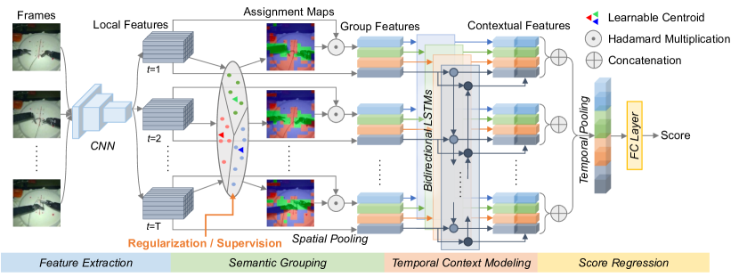
Figure 1: The proposed framework, Video Semantic Aggregation (ViSA), for surgical skill assessment. It aggregates local CNN features over space and time using semantic clues embedding in the video. We aim to group video parts according to semantics, e.g., tools, tissue and background, and model the temporal relationship for different parts separately via this framework. We also investigate the regularization or additional supervision to the group results for enhancement.

2 Methodology

As shown in Fig. 1, for each video, our framework takes frames from a fixed number of timesteps as input and predicts the final skill assessment score through the following 4 stacked modules: (1) the Feature Extraction Module (FEM) that produces feature maps for each timestep (Sec. 2.1); (2) the Semantic Grouping Module (SGM) that aggregates local features into a specified number of groups based on the embedded semantics (Sec. 2.2); (3) the Temporal Context Modeling Module (TCMM) that models the contextual relationship for the feature series of each group (Sec. 2.3); (4) the Score Prediction Module (SPM) that regresses the final score based on the spatiotemporally aggregated features (Sec. 2.4).

2.1 Feature Extraction Module

Our framework first feeds the input frames to CNNs to collect the intermediate layer responses as the feature maps for the subsequent processing. We stack the feature maps for one video along the temporal dimension and registered them as $\bm{X}\in\mathbb{R}^{T\times H\times W\times C}$, where $T$ is the number of timesteps, $H,W$ represents the height and width of each feature map, and $C$ is the number of channels. $\bm{X}$ can also be seen as a group of local features, where each feature is indexed by the temporal and spatial position $t,i,j$ as $\bm{X}_{tij}\in\mathbb{R}^{C}$.

2.2 Semantic Grouping Module

This module aggregates the extracted features $\bm{X}$ into a fixed number of groups, with each representing a specific kind of semantic meaning. Taking inspirations from [5, 7], we achieve this by clustering all local CNN features across the entire spatiotemporal range of the video according to $K$ learnable vectors $\bm{D}=[\bm{d}_{1},\cdots,\bm{d}_{K}]^{\top}\in\mathbb{R}^{K\times C}$ which record the feature centroid of each group (drawn as colored triangles in Fig. 1).

2.2.1 Local Feature Assignment

We softly assign local features to different groups by computing the assignment possibilities $\bm{P}\in\mathbb{R}^{T\times H\times W\times K}$ subject to $\bm{P}^{k}_{tij}=\frac{\text{exp}(-\parallel(\bm{X}_{tij}-\bm{d}_{k})/\sigma_{k}\parallel^{2}_{2})}{\sum_{k^{\prime}}\text{exp}(-\parallel(\bm{X}_{tij}-\bm{d}_{k^{\prime}})/\sigma_{k^{\prime}}\parallel^{2}_{2})}$. Component $\bm{P}^{k}_{tij}$ represents the possibility of assigning the local CNN feature $\bm{X}_{tij}$ to the $k^{\text{th}}$ semantic group. $\sigma_{k}\in(0,1)$ is a learnable factor to adjust feature magnitudes and smooth the assignment for each semantic group. Taking the index of the group with the maximum possibility at each position, we obtain the assignment maps $\bm{A}\in\mathbb{R}^{T\times H\times W}$ with component $\bm{A}_{tij}=\operatorname*{argmax}_{k=1,\dots,K}\bm{P}^{k}_{tij},\forall t,i,j.$ As shown in Fig. 1, the assignment maps visualize the correspondence between video parts and semantic groups.

2.2.2 Group Feature Aggregation

For each timestep, we aggregate the corresponding local features according to the soft-assignment results and generate an abstract representation for each semantic group. We first calculate the normalized residual between the centroid and the averaged local features weighted by assignment possibilities as $\bm{z}^{k}_{t}=\frac{\bm{z}^{\prime k}_{t}}{\parallel\bm{z}^{\prime k}_{t}\parallel_{2}}$, where $\bm{z}^{\prime k}_{t}=\frac{1}{\sigma_{k}}\big{(}\sum_{ij}\frac{{\bm{P}^{k}_{tij}\bm{X}_{tij}}}{\sum_{ij}{\bm{P}^{k}_{tij}}}-\bm{d_{k}}\big{)}$. Then we get one group feature $\bm{g}^{k}_{t}$ for capturing the abstract information of the $k^{\text{th}}$ semantics at each timestep by transforming $\bm{z}^{k}_{t}$ with a sub-network $f_{g}$ consisting of 2 linear transformations as $\bm{g}_{t}^{k}=f_{g}(\bm{z}^{k}_{t})$.

2.2.3 Group Existence Regularization

To avoid most local features being allocated to one single group, we leverage a regularization term [7] to retain the even distribution among groups at every timestep. Specifically, it regularizes the existence of each group by constraining the max assignment probability of one group, i.e., $\hat{p}_{t}^{k}:=\max_{i,j}\bm{P}_{t,i,j}^{k}$, as close to 1.0 as possible. Instead of tightly constraining $\hat{p}_{t}^{k}$ to an exact number, the regularization term restricts the cumulative distribution function of $\hat{p}^{k}$ to follow a beta distribution. We implement the regularization term as $\mathcal{L}_{exist}=\sum_{i=1}^{T}\Big{(}\log\big{(}\bm{p}^{\star k}_{i}+\epsilon\big{)}-\log\big{(}F^{-1}(\frac{2i-1}{2T};\alpha,\beta)+\epsilon\big{)}\Big{)}$. $\bm{p}^{\star k}=\text{sort}([\hat{p}_{1}^{k}\cdots\hat{p}_{T}^{k}])$ arranges the maximum assignment probabilities of the $k^{\text{th}}$ group at all timesteps in ascending order. $\alpha$=1 and $\beta$=0.001 control the shape of the beta distribution. $\epsilon$ is a small value for numerical stability. $F^{-1}(\frac{2i-1}{2T};\alpha,\beta)$ means an inverse cumulative beta distribution function, which returns the $i^{\text{th}}$ element of the sequence of $T$ probability values obeying this distribution.

2.3 Temporal Context Modeling Module

For each obtained semantic group feature series, this module aims to keep track of its long-term dependencies and model their contextual relationships independently in a recurrent manner. As shown in Fig. 1, we achieve this by employing $K$ bidirectional LSTMs (BiLSTMs): $\overrightarrow{\bm{h}}_{t}^{k}=\overrightarrow{L}^{k}(\overrightarrow{\bm{h}}_{t-1}^{k},\bm{g}_{t}^{k})$, $\overleftarrow{\bm{h}}_{t}^{k}=\overleftarrow{L}^{k}(\overleftarrow{\bm{h}}_{t+1}^{k},\bm{g}_{t}^{k})$, where $\overrightarrow{L}^{k}$ and $\overleftarrow{L}^{k}$ denote the $k^{\text{th}}$ forward and backward LSTMs respectively. The output vectors of every timestep $\overrightarrow{\bm{h}}_{t}^{k}$ and $\overleftarrow{\bm{h}}_{t}^{k}$ from the two directions are further concatenated to form the contextual feature $\bm{c}_{t}^{k}=[\overrightarrow{\bm{h}}_{t}^{k\top},\overleftarrow{\bm{h}}_{t}^{k\top}]^{\top}$. To prevent the potential information loss caused by the separated modeling (e.g., the interaction between groups), we also employ another BiLSTM to model the global features $[\bm{x}_{1}\cdots\bm{x}_{T}]$ which are obtained by taking spatial average pooling on $\bm{X}$. $\bm{c}_{t}^{0}$ denotes the generated contextual features by this additional BiLSTM.

2.4 Score Prediction Module

This module concatenates the contextual features $\bm{c}_{t}^{k}$ of different semantic groups at the same timestep into a vector, followed by an average pooling on these vectors across the temporal dimension. The pooled vector is finally regressed to the skill score $s$ by $f_{s}$, a fully connected layer. We formulate this module mathematically as follows: $\hat{s}=f_{s}(\frac{1}{T}\sum_{t=1}^{T}[\bm{c}_{t}^{0\top}\cdots\bm{c}_{t}^{K\top}]^{\top})$. The training loss function is defined as: $\mathcal{L}=(s-\hat{s})^{2}+\lambda\mathcal{L}_{exist},$ with $s$ denoting the ground-truth score. The scalar $\lambda=10$ controls the contribution of the group existence regularization.

2.5 Incorporating Auxiliary Supervision Signals

Our unique representation aggregation strategy also allows enhancing the feature grouping results by incorporating additional supervision signals to assign specific known semantic information to certain groups. Specifically, we propose a Heatmap Prediction Module (HPM), which takes as input the CNN feature maps $\bm{X}$ and the assignment possibility maps $\bm{P}^{m}$ of the $m^{\text{th}}$ group. The module predicts the positions of the specified semantics by generating heatmaps $\hat{\bm{H}}=f_{HPM}(\bm{P}^{m}\odot\bm{X})\in\mathbb{R}^{T\times H\times W}$, where $\odot$ denotes the Hadamard product, and $f_{HPM}$ is composed of one basic $1\times 1$ conv block followed by a Sigmoid function. Assuming the 2D positions of the specified semantics is known, we generate the position heatmaps $\bm{H}\in\mathbb{R}^{T\times H\times W}$ from the 2D positions as the supervision signal. The framework integrating HPM is trained by the loss function with an extra position regularization $\mathcal{L^{\prime}}=(s-\hat{s})^{2}+\lambda_{1}\mathcal{L}_{exist}+\lambda_{2}\mathcal{L}_{pos}$, where $\mathcal{L}_{pos}$ computes the binary cross entropy between $H$ and $\hat{H}$ and $\lambda_{1}$=10, $\lambda_{2}$=20.

3 Experiments

Table 1: Baseline comparison on JIGSAWS. We report the Spearman’s Rank Correlations by three cross-validation schemes on every task. K: Kinematic data, V: video frames, *: extra annotations such as surgical gestures are utilized.

Input Method Task & Scheme KT NP SU Avg. LOSO LOUO 4-Fold LOSO LOUO 4-Fold LOSO LOUO 4-Fold LOSO LOUO 4-Fold K SMT-DCT-DFT [26] 0.70 0.73 - 0.38 0.23 - 0.64 0.10 - 0.59 0.40 - DCT-DFT-ApEn [26] 0.63 0.60 - 0.46 0.25 - 0.75 0.37 - 0.63 0.41 - V ResNet-LSTM [23] 0.52 0.36 - 0.84 0.33 - 0.73 0.67 - 0.72 0.59 - C3D-LSTM [16] 0.81 0.60 - 0.84 0.78 - 0.69 0.59 - 0.79 0.67 - C3D-SVR [16] 0.71 0.33 - 0.75 -0.17 - 0.42 0.37 - 0.65 0.18 - USDL [18] - - 0.61 - - 0.63 - - 0.64 - - 0.63 MUSDL [18] - - 0.71 - - 0.69 - - 0.71 - - 0.70 *S3D [25] 0.64 0.14 - 0.57 0.35 - 0.68 0.03 - - - - *ResNet-MTL-VF [23] 0.63 0.72 - 0.73 0.48 - 0.79 0.68 - 0.73 0.64 - *C3D-MTL-VF [23] 0.89 0.83 - 0.75 0.86 - 0.77 0.69 - 0.75 0.68 - V+K JR-GCN [14] - 0.19 0.75 - 0.67 0.51 - 0.35 0.36 - 0.40 0.57 AIM [3] - 0.61 0.82 - 0.34 0.65 - 0.45 0.63 - 0.47 0.71 MultiPath-VTP [13] - 0.58 0.78 - 0.62 0.76 - 0.45 0.79 - 0.56 0.78 *MultiPath-VTPE [13] - 0.59 0.82 - 0.65 0.76 - 0.45 0.83 - 0.57 0.80 V ViSA 0.92 0.76 0.84 0.93 0.90 0.86 0.84 0.72 0.79 0.90 0.81 0.83

Dataset We evaluate ViSA framework on 2 datasets for surgical skill assessment: JIGSAWS [4] and HeiChole [22]. JIGSAWS is a widely used dataset consisting of 3 elementary surgical tasks: Knot Tying (KT), Needle Passing (NP), and Suturing (SU). Each task contains more than 30 trials performed on the da Vinci surgical system, which is rated from 6 aspects. Following [23, 13, 26], the sum score is used as the ground truth. We validate our method on every task by 3 kinds of cross-validation schemes: Leave-one-supertrial-out (LOSO), Leave-one-user-out (LOUO) and 4-Fold [14, 18, 3]. HeiChole is a challenging dataset containing 24 endoscopic videos in real surgical environments for laparoscopic cholecystectomy. For each video, 2 clips of the phases calot triangle dissection and gallbladder dissection are provided with skill scores from 5 domains. We use the sum score as the ground truth. We train and validate our framework on the 48 video clips by 4-fold cross-validation with a 75/25 partition ratio.

Evaluation Metric For JIGSAWS, since previous works [23, 13] only included the results on Spearman’s Rank Correlation (Corr), we report the validation correlations averaged on all folds for one task and compute the average correlation across tasks by Fisher’s z-value [15] for baseline comparison. We incorporate the results on Mean Absolute Error (MAE) in ablation studies. For HeiChole, we report both the correlation and MAE averaged on all folds. The reported results are averaged on multiple runs with different random seeds.

Implementation Details We employ R(2+1)D-18 [20] pre-trained on Kinetic-400 dataset [8] as the feature extractor and take the response of the 4${}^{\text{th}}$ convolutional block as the 3D spatiotemporal feature. Since each 3D feature is extracted from 4 frames, we divide each video into $T$ segments and sample a 4-frame snippet from each. $T$ is set to 32 on JIGSAWS videos and 64 on longer HeiChole videos. Each sampled frame is resized to $160\times 120$ and crop the $112\times 112$ region in the center as input. Hence, the spatial size of the extracted CNN feature maps is $14\times 14$. We also investigate 2D-CNNs feature extractor by using ResNet-18 pre-trained on ImageNet. Since the surgical scenes in our experiments explicitly include 3 parts: represented by tools, tissues, and background, we initialize the number of semantic groups $K=3$. It should be set according to the scene complexity and fine-tuned based on the experiment results. The framework is implemented by PyTorch. We use SDG optimizer with mean squared error loss. Models are trained in 40 epochs with a batch size of 4. Learning rates are initialized as 3e-5 and decayed by 0.1 times for every 20 epochs.

Table 2: Results on HeiChole. Baseline frameworks are newly constructed and compared with ViSA by MAE and Corr metrics.

Method MAE Corr R2D-18 + FC 1.56 0.32 R2D-18 + LSTM 1.42 0.15 R(2+1)D-18 + FC 1.54 0.29 R(2+1)D-18 + LSTM 1.33 0.31 ViSA (R2D-18) 1.27 0.46 ViSA (R(2+1)D-18) 1.27 0.46

Table 3: Ablation studies on JIGSAWS. We train frameworks across videos of three tasks and report Corr and MAEs on LOSO and LOUO settings. K denotes the number of Groups.

FEM SGM TCMM K LOSO LOUO MAE Corr MAE Corr R2D-18 ✗ BiLSTMs - 3.40 0.65 3.53 0.67 R2D-18 ✓ BiLSTMs 3 3.27 0.80 3.42 0.74 R(2+1)D-18 ✓ LSTMs 3 2.41 0.83 3.23 0.78 R(2+1)D-18 ✓ Transformer 3 3.02 0.76 3.27 0.68 R(2+1)D-18 ✗ BiLSTMs - 2.90 0.73 3.30 0.72 R(2+1)D-18 ✓ BiLSTMs 2 2.34 0.84 3.07 0.72 R(2+1)D-18 ✓ BiLSTMs 4 2.32 0.85 2.68 0.79 R(2+1)D-18 ✓ BiLSTMs 3 2.24 0.86 2.86 0.76

3.1 Baseline Comparison

Tab. 1 shows the quantitative baseline comparison results of ViSA on JIGSAWS. Baseline results are taken from previous papers. We find that ViSA outperforms many competitive methods on most tasks and cross-validation schemes. ViSA has a CNN-RNN framework akin to C3D-MTL-VF [23] but surpasses it with obvious margins on most LOSO and LOUO metrics. On 4-Fold, ViSA achieves nearly equivalent performance as MultiPath-VTPE [13] which needs extra input sources such as frame-wise surgical gestures information and tool movement paths. For HeiChole, since no baseline is available, we newly constructed four basic frameworks by combining 2D or 3D CNN feature extractors with temporal aggregation modules of fully connected layers (FC) or LSTMs, which share similar CNN architectures and pre-trained parameters as ViSA. Tab. 3 shows the out-performance of ViSA against the four baselines on both metrics.

JIGSAWS				HeiChole

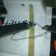
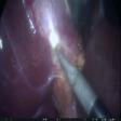
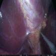
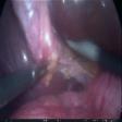
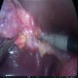
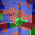
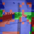
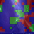
Figure 2: Visualization of the assignment maps that display the correspondence between video parts and different semantic groups.

Frames
Without SGM
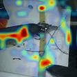
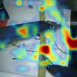
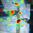
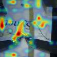
With SGM

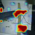
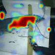
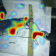
Figure 3: Visual explanations generated by Grad-CAM. SGM facilitates the concentration on the tools and discarding the unrelated background regions.

Without Position Supervision
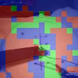
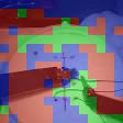
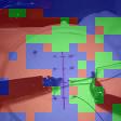
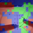
Heatmaps for Position Supervision
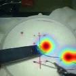
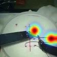
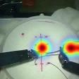
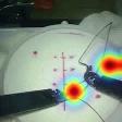
With Position Supervision

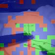
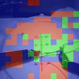
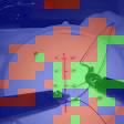
Figure 4: Improved semantic grouping results after using the tool position supervision. Green regions turn to focus on tool clips after using supervision.

3.2 Assignment Visualization

Fig. 2 visualizes the assignment maps generated by ViSA on two datasets. The three semantic groups generally correspond to the tools, the manipulated tissues, and the background regions as expected. Notably, ViSA gets this assignment result without taking any supervision of semantics, which further indicates its effectiveness in modeling surgical actions over spatiotemporal dimensions.

3.3 Ablation Study

We also conduct the ablation analysis on three key components and one hyper-parameter of ViSA: Feature Extraction Module (FEM), Semantic Grouping Module (SGM), Temporal Context Modeling Module (TCMM), and the number of semantic groups (K). Referring to [23], we train and validate the ablative frameworks across videos of 3 JIGSAWS tasks by forming them together, in order for stable results on more samples. Results in Tab. 3 indicate that: (1) leveraging SGM boosts the performance on either R(2+1)D-18 or R2D-18; (2) BiLSTMs perform better than LSTMs and Transformer [21] in modeling temporal context; (3) increasing $K$ from 2 to 3 causes more improvements than raising it from 3 to 4, which indicates separating semantics into 3 groups fits the JIGSAWS dataset. Transformer consists of two layers of LayerNorm+Multi-Head-Attention+MLP. Considering the data-hungry nature of Transformer [6], we attribute its unremarkable performance to the small amount of training data.

Fig. 4 presents the visual explanation results generated by the post-hoc interpretation method Grad-CAM [12, 17] which localizes the input regions used by networks for decision making. Compared to the network without using the semantic grouping module (SGM), the full framework employs more task-related parts for predictions (e.g., regions about robotic tools) and discards many unrelated regions. We attribute the improvement to explicitly discovering different video parts and modeling their spatiotemporal relationship in our framework.

3.4 Improved Performance with Supervision

ViSA also supports the explicit supervision on the grouping process that allocates specific semantics to certain expected groups. On JIGSAWS, the kinematic data recording the positions of two robotic clips in 3D space is available. We first approximate the two clips’ positions on the 2D image plane by projecting their 3D kinematic positions with estimated transformation matrix. Then we generate the heatmaps $\bm{H}\in\mathbb{R}^{T\times H\times W}$ from the 2D positions and train the framework as described in Sec. 2.5. Fig. 4 illustrates one example of the generated position heatmaps. On the Suturing task, we achieve the improvement in average validation correlations as $0.84\rightarrow 0.87$, $0.72\rightarrow 0.80$ and $0.80\rightarrow 0.86$ on LOSO, LOUO, and 4-Fold schemes respectively. In Fig. 4, we show one imperfect assignment maps generated by the model without supervision and its corresponding maps after using the position supervision. Although the position supervision is not fully precise, it still benefits the network to discover the tools’ features. Hence, in Fig. 4, the green regions become less noisy and are guided to the regions of tool clips and tool-tissue interactions after using the supervision.

4 Conclusion

In this paper, a novel framework called ViSA is proposed to predict the skill score from surgical videos by discovering and aggregating different semantic parts across spatiotemporal dimensions. The framework can achieve competitive performance on two datasets: JIGSAWS and HeiChole as well as support explicit supervision on the feature semantic grouping for performance improvement.

4.0.1 Acknowledgment.

This work is supported by JST AIP Acceleration Research Grant Number JPMJCR20U1, JSPS KAKENHI Grant Number JP20H04205, JST ACT-X Grant Number JPMJAX190D, JST Moonshot R&D Grant Number JPMJMS2011, Fundamental Research Funds for the Central Universities under Grant DUT21RC(3)028 and a project commissioned by NEDO.

References

- [1] Fawaz, H.I., Forestier, G., Weber, J., Idoumghar, L., Muller, P.A.: Evaluating surgical skills from kinematic data using convolutional neural networks. In: International Conference on Medical Image Computing and Computer-Assisted Intervention. pp. 214–221. Springer (2018)
- [2] Funke, I., Mees, S.T., Weitz, J., Speidel, S.: Video-based surgical skill assessment using 3d convolutional neural networks. International Journal of Computer Assisted Radiology and Surgery 14(7), 1217–1225 (2019)
- [3] Gao, J., Zheng, W.S., Pan, J.H., Gao, C., Wang, Y., Zeng, W., Lai, J.: An asymmetric modeling for action assessment. In: European Conference on Computer Vision. pp. 222–238. Springer (2020)
- [4] Gao, Y., Vedula, S.S., Reiley, C.E., Ahmidi, N., Varadarajan, B., Lin, H.C., Tao, L., Zappella, L., Béjar, B., Yuh, D.D., et al.: Jhu-isi gesture and skill assessment working set (jigsaws): A surgical activity dataset for human motion modeling. In: MICCAI workshop: M2cai. vol. 3, p. 3 (2014)
- [5] Girdhar, R., Ramanan, D., Gupta, A., Sivic, J., Russell, B.: Actionvlad: Learning spatio-temporal aggregation for action classification. In: Proceedings of the IEEE Conference on Computer Vision and Pattern Recognition. pp. 971–980 (2017)
- [6] Hassani, A., Walton, S., Shah, N., Abuduweili, A., Li, J., Shi, H.: Escaping the big data paradigm with compact transformers. arXiv preprint arXiv:2104.05704 (2021)
- [7] Huang, Z., Li, Y.: Interpretable and accurate fine-grained recognition via region grouping. In: Proceedings of the IEEE Conference on Computer Vision and Pattern Recognition. pp. 8662–8672 (2020)
- [8] Kay, W., Carreira, J., Simonyan, K., Zhang, B., Hillier, C., Vijayanarasimhan, S., Viola, F., Green, T., Back, T., Natsev, P., et al.: The kinetics human action video dataset. arXiv preprint arXiv:1705.06950 (2017)
- [9] Kelly, J.D., Petersen, A., Lendvay, T.S., Kowalewski, T.M.: Bidirectional long short-term memory for surgical skill classification of temporally segmented tasks. International Journal of Computer Assisted Radiology and Surgery 15(12), 2079–2088 (2020)
- [10] Lavanchy, J.L., Zindel, J., Kirtac, K., Twick, I., Hosgor, E., Candinas, D., Beldi, G.: Automation of surgical skill assessment using a three-stage machine learning algorithm. Scientific reports 11(1), 1–9 (2021)
- [11] Li, Z., Huang, Y., Cai, M., Sato, Y.: Manipulation-skill assessment from videos with spatial attention network. In: Proceedings of the IEEE/CVF International Conference on Computer Vision Workshops. pp. 0–0 (2019)
- [12] Li, Z., Wang, W., Li, Z., Huang, Y., Sato, Y.: Spatio-temporal perturbations for video attribution. IEEE Transactions on Circuits and Systems for Video Technology 32(4), 2043–2056 (2021)
- [13] Liu, D., Li, Q., Jiang, T., Wang, Y., Miao, R., Shan, F., Li, Z.: Towards unified surgical skill assessment. In: Proceedings of the IEEE/CVF Conference on Computer Vision and Pattern Recognition. pp. 9522–9531 (2021)
- [14] Pan, J.H., Gao, J., Zheng, W.S.: Action assessment by joint relation graphs. In: Proceedings of the IEEE/CVF International Conference on Computer Vision. pp. 6331–6340 (2019)
- [15] Parmar, P., Morris, B.: Action quality assessment across multiple actions. In: IEEE Winter Conference on Applications of Computer Vision. pp. 1468–1476 (2019)
- [16] Parmar, P., Tran Morris, B.: Learning to score olympic events. In: Proceedings of the IEEE Conference on Computer Vision and Pattern Recognition Workshops. pp. 20–28 (2017)
- [17] Selvaraju, R.R., Cogswell, M., Das, A., Vedantam, R., Parikh, D., Batra, D.: Grad-cam: Visual explanations from deep networks via gradient-based localization. In: Proceedings of the IEEE/CVF International Conference on Computer Vision (2017)
- [18] Tang, Y., Ni, Z., Zhou, J., Zhang, D., Lu, J., Wu, Y., Zhou, J.: Uncertainty-aware score distribution learning for action quality assessment. In: Proceedings of the IEEE Conference on Computer Vision and Pattern Recognition (2020)
- [19] Tao, L., Elhamifar, E., Khudanpur, S., Hager, G.D., Vidal, R.: Sparse hidden markov models for surgical gesture classification and skill evaluation. In: International Conference on Medical Image Computing and Computer-Assisted Intervention. pp. 167–177. Springer (2012)
- [20] Tran, D., Wang, H., Torresani, L., Ray, J., LeCun, Y., Paluri, M.: A closer look at spatiotemporal convolutions for action recognition. In: Proceedings of the IEEE Conference on Computer Vision and Pattern Recognition. pp. 6450–6459 (2018)
- [21] Vaswani, A., Shazeer, N., Parmar, N., Uszkoreit, J., Jones, L., Gomez, A.N., Kaiser, Ł., Polosukhin, I.: Attention is all you need. Advances in Neural Information Processing Systems 30 (2017)
- [22] Wagner, M., Müller-Stich, B.P., Kisilenko, A., Tran, D., Heger, P., Mündermann, L., Lubotsky, D.M., Müller, B., Davitashvili, T., Capek, M., et al.: Comparative validation of machine learning algorithms for surgical workflow and skill analysis with the heichole benchmark. arXiv preprint arXiv:2109.14956 (2021)
- [23] Wang, T., Wang, Y., Li, M.: Towards accurate and interpretable surgical skill assessment: A video-based method incorporating recognized surgical gestures and skill levels. In: International Conference on Medical Image Computing and Computer-Assisted Intervention. pp. 668–678. Springer (2020)
- [24] Wang, Z., Fey, A.M.: Deep learning with convolutional neural network for objective skill evaluation in robot-assisted surgery. International Journal of Computer Assisted Radiology and Surgery 13(12), 1959–1970 (2018)
- [25] Xiang, X., Tian, Y., Reiter, A., Hager, G.D., Tran, T.D.: S3d: Stacking segmental p3d for action quality assessment. In: IEEE International Conference on Image Processing. pp. 928–932. IEEE (2018)
- [26] Zia, A., Essa, I.: Automated surgical skill assessment in rmis training. International Journal of Computer Assisted Radiology and Surgery 13(5), 731–739 (2018)
- [27] Zia, A., Sharma, Y., Bettadapura, V., Sarin, E.L., Essa, I.: Video and accelerometer-based motion analysis for automated surgical skills assessment. International Journal of Computer Assisted Radiology and Surgery 13(3), 443–455 (2018)