Abstract

We have already shown how a modified Friedmann equation, originating from a model of the Universe built from a certain $W_{3}$ algebra, is able to explain the difference between the Hubble constants extracted from CMB data and from local measurements. In this article we show that the same model also describes aspects of the large scale structure of the Universe well.

1 Introduction

In previous articles [1, 2] we have advocated a modified Friedmann equation which is able to resolve the $H_{0}$ tension and where the cosmological constant is assumed to be zero at present time due to Coleman’s mechanism [3]. The modified Friedmann equation arose from a “model of the Universe” suggested in [4]. One feature of this model is that the late time exponential expansion of the universe is not caused by the cosmological constant, but by a new constant related to the creation of baby universes. The possibility of creating such baby universe reflects the fractal structure of spacetime and is not related to the vacuum energy dictated by the cosmological constant. It is our hope that we will be able to estimate the order of this constant related to the creation of baby universes. However, it is not yet possible, and one should view our modified Friedmann equation as a phenomenological equation with one free parameter, $B$, in the same way as the ordinary Friedmann equation has the cosmological constant $\Lambda$ as a free parameter. Like $\Lambda$, the parameter $B$ has to be small in order that the model agrees with observations. Thus the physics of the modified Friedmann equation as well as that of the ordinary Friedmann equation are independent of $B$ and $\Lambda$ for all questions related to observations refering to times earlier than the time $t_{\rm LS}$ of last scattering. In this sense our model belongs to a class of models modifying the late time cosmology [5, 6, 7], and in fact our phenomenological model becomes similar to models where one puts in by hand a time-dependent dark energy equation of state for small values of $z$, parametrized in such a way as to ease the $H_{0}$ or the $S_{8}$ tension. In these models, in order to accommodate larger value of $H_{0}$ than the value predicted by the Planck data using the $\Lambda$CDM model [8], one is led to values of $w(z)<-1$ in some regions of $z$ [6, 9, 10] and since a larger value of $H_{0}$ leads to less growth of density fluctuations for small $z$, it has been pointed out that one at the same time might ease the $S_{8}$ tension [5, 6].

As noticed in [2] the situation is the same in our model: our “effective” $w(z)<-1$ (and approaches $-1$ for late times), and the purpose of this article is to show that for precisely the same values of our baby universe parameter $B$ which ease the $H_{0}$ tension, we also agree with a number of other late time cosmological observations while assuming the same physics as the Planck Collaboration at and before the time of last scattering (we denote this physics CMB physics).

2 The modified Friedmann equation and large scale structures

In [1] we showed that our modified Friedmann equation is

$$\left(\frac{\dot{a}}{a}\right)^{2}=\frac{\kappa\rho}{3}+\frac{Ba}{\dot{a}}\frac{(1+3F(x))}{F^{2}(x)},\quad x:=\frac{Ba^{3}}{\dot{a}^{3}},\quad F^{2}(x)-F^{3}(x)=x.$$ (1)

In (1) $a(t)$ is the scale factor of the Universe. The second term on the rhs of equation (1) is a term that replaces the term $\Lambda/3$ which would be present of there was a cosmological constant. $x$ has to be less than or equal to 4/27 and one has to choose the solution $F(x)$ to the third order equation which is larger than or equal to 2/3. Despite the missing cosmological constant, the solution $a(t)$ will grow exponentially for large time as $a(t)\;\propto\;{\rm e}^{(27B/4)^{1/3}t}$. However, the replacement of $\Lambda/3$ with the more complicated term which is a function of $a(t)$ makes it possible to have physics agreeing with both the CMB measurements which refer to time $t_{\rm LS}$ and the small $z$ measurements which refer to physics at present time. In [1] we showed that an agreement could be obtained for $H(z)$, the Hubble constant as a function of the redshift $z$. Here we will show that for the values of $B$ determined in [1], which led to the resolution of the Hubble constant tension, our model, without further modifications, also agrees with other late time cosmological observations.

2.1 Baryon Acoustic Oscillations

The baryon acoustic oscillations (BAO) are fluctuations in the baryon density caused by the baryon acoustic oscillation in the early universe. In BAO an important observable is the inverse of the angular diameter distance

$$\frac{1}{\theta}\,:=\,\frac{D_{\rm V}(z)}{r_{\rm s}}.$$ (2)

In this equation $D_{\rm V}(z)$ is a distance measure and $r_{\rm s}$ is the co-moving sound horizon at $t_{\rm drag}$. More precisely, $D_{\rm V}(z)$ is a kind of the average of three directions of distance, i.e.

$$D_{\rm V}(z)\,:=\,\sqrt[3]{zD_{\rm H}(z)\big{(}D_{\rm M}(z)\big{)}^{2}}$$ (3)

where

$$zD_{\rm H}(z)\,:=\,\frac{c{\hskip 1.11206pt}z}{H(z)}\,,\qquad\quad D_{\rm M}(z)\,:=\,\int_{0}^{{\hskip 0.38922pt}z}\!\frac{c{\hskip 1.11206pt}{\rm d}z^{\prime}}{H(z^{\prime})}\,.$$ (4)

$r_{\rm s}$ is defined by

$$r_{\rm s}\,=\,\int_{0}^{{\hskip 0.77844pt}t_{\rm drag}}\!{\rm d}t{\hskip 1.11206pt}\,\frac{a(t_{\rm drag})}{a(t)}{\hskip 1.11206pt}\,c_{\rm s}(t)\,,$$ (5)

where $c_{\rm s}$ is the speed of sound,

$$c_{\rm s}(t)\,=\,\frac{c}{\sqrt{3\big{(}1+R(t)\big{)}}}\,,\qquad\quad R(t)\,:=\,\frac{3{\hskip 0.55603pt}\rho_{{\hskip 0.38922pt}\rm b}(t)}{4{\hskip 0.55603pt}\rho_{\gamma}(t)}\,.$$ (6)

$\rho_{{\hskip 0.38922pt}\rm b}(t)$ is the baryon density and $\rho_{\gamma}(t)$ is the photon density. The baryon drag ends at $t_{\rm drag}<t_{\rm LS}$. Thus $r_{\rm s}$, as defined by eq.  (5), is determined by physical phenomena before $t_{\rm LS}$, and according to our assumptions the value of $r_{\rm s}$ in our model (which we in the following will label with a superscript $(B)$, for the baby universe coupling constant appearing in (1)) will therefore coincide with the Planck value obtained from the $\Lambda$CDM model:

$$r_{\rm s}^{\rm(B)}=r_{\rm s}^{\rm(SC)}=r_{\rm s}^{\rm(CMB)}\,=\,147.05\pm 0.30\ [\,{\rm Mpc}\,]\,.$$ (7)

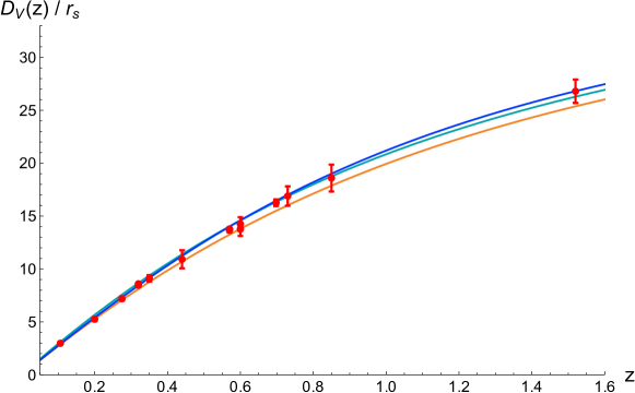
Figure 1: $z$ plotted versus  $D_{\rm V}(z)/r_{\rm s}$ for our model (blue), for the Planck data $\Lambda$CDM model (green) and the $\Lambda$CDM model with late time $H_{0}=73.04$ (orange). The data point error bars are from table 1.

Fig. 1 shows $D_{\rm V}(z)/r_{\rm s}$, calculated from our model with $H_{0}=73.04\pm 1.04$ (which, as already mentioned, is the latest value published by the SH0ES team [11]), for the $\Lambda$CDM model with $\Lambda$ and $H_{0}$ given by the Planck collaboration, and for the $\Lambda$CDM model where $H_{0}=73.04$ and where the corresponding $\Lambda_{\rm SC}$ is determined from the $\Lambda$CDM model by requiring that $z(t_{\rm LS})=1089.95$. The reason we consider this third model, denoted SC for “standard candles” used to measure distances for small $z$, is that it is the $\Lambda$CDM model where $H(z)$ is calculated using precisely the same assumptions as for our baby universe model. The data points are from Table 1 in the Appendix and lead to reduced $\chi^{2}$ values

$$(\chi_{\rm red}^{\rm(B)})^{2}=1.0\,,\qquad\big{(}\chi_{\rm red}^{\rm(SC)}\big{)}^{2}=4.7\,,\qquad\big{(}\chi_{\rm red}^{\rm(CMB)}\big{)}^{2}=1.7\,.$$ (8)

We note that the $\Lambda$CDM model with $\Lambda_{\rm SC}$ and $H_{0}=73.04$ fits the data less well than our model.

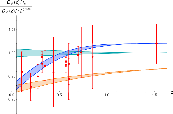
Figure 2: $z$ versus $\frac{D_{\rm V}(z)/r_{\rm s}}{D_{\rm V}^{\rm(CMB)}(z)/r_{\rm s}^{\rm(CMB)}}$ for the three models: our model (blue), Planck data $\Lambda$CDM model (green) and late time $\Lambda$CDM model (orange). The widths of the curves indicate the $1\sigma$ error bars related to the fits. The error bars of the data are from table 1.

To emphasize the difference for the three models Fig. 2 shows the graphs ${D_{\rm V}(z)}/{r_{\rm s}}$ divided by the central graph values of ${D_{\rm V}^{\rm(CMB)}(z)}/{r_{\rm s}^{\rm(CMB)}}$. The message to take away is that our model fits the data well.

2.2 The growth of fluctuations

The matter density fluctuation $\delta_{\rm m}(\mbox{{\boldmath$x$}},t)$ is defined by

$$\delta_{\rm m}(\mbox{{\boldmath$x$}},t)\,:=\,\frac{\rho_{\rm m}(\mbox{{\boldmath$x$}},t)}{\rho_{\rm m}(t)}-1\qquad\hbox{and}\qquad\rho_{\rm m}(t)\,:=\,\frac{\int\!{\rm d}^{3}x{\hskip 1.11206pt}\rho_{\rm m}(\mbox{{\boldmath$x$}},t)}{\int\!{\rm d}^{3}x}\,.$$ (9)

In the linear approximation, the matter density fluctuation $\delta_{\rm m}(\mbox{{\boldmath$x$}},t)$ obeys the differential equation

$$\frac{{\rm d}}{{\rm d}t}\Big{(}\big{(}a(t)\big{)}^{2}\frac{{\rm d}}{{\rm d}t}\delta_{\rm m}(\mbox{{\boldmath$x$}},t)\Big{)}\,=\,\frac{\kappa}{2}\big{(}a(t)\big{)}^{2}\rho_{\rm m}(t){\hskip 0.55603pt}\delta_{\rm m}(\mbox{{\boldmath$x$}},t){\hskip 1.11206pt}+{\hskip 1.11206pt}{\cal O}(B)\,.$$ (10)

We here assume that $\delta_{\rm m}(\mbox{{\boldmath$x$}},t)$ is decoupled at all times from $t_{\rm LS}$ to the present time $t_{0}$ as

$$\delta_{\rm m}(\mbox{{\boldmath$x$}},t)\,=\,F_{\rm m}(t)\Delta_{\rm m}(\mbox{{\boldmath$x$}})$$ (11)

where $F_{\rm m}(t)$ is the growth factor which represents the growth of fluctuation and $\Delta_{\rm m}(\mbox{{\boldmath$x$}})$ is the fluctuation at a certain time. Then we have the following differential equation for $F_{\rm m}(t)$:

$$\frac{{\rm d}}{{\rm d}t}\bigg{(}\big{(}a(t)\big{)}^{2}\frac{{\rm d}}{{\rm d}t}F_{\rm m}(t)\Big{)}=\frac{\kappa}{2}\big{(}a(t)\big{)}^{2}\rho_{\rm m}(t){\hskip 0.55603pt}F_{\rm m}(t)\,.$$ (12)

Here we have assumed the contribution from the production of baby universes is negligible, i.e. we have deleted ${\cal O}(B)$ in eq. (10). The boundary conditions of the growth factor $F_{\rm m}(t)$ are

$$F_{\rm m}(t_{0})\,=\,1\qquad\hbox{and}\qquad f_{\rm m}(t_{\rm LS})\,=\,1$$ (13)

where $f_{\rm m}(t)$ is the growth rate defined by

$$f_{\rm m}(t)\,:=\,\frac{{\rm d}\log F_{\rm m}(t)}{{\rm d}\log a(t)},$$ (14)

and where $t_{0}$ refers to the present time (and $t_{\rm LS}$ as before to the time of last scattering).

One now introduces the average of fluctuation inside the sphere with radius $R$:

$$\sigma_{R}(t)\,:=\,\sqrt{\bigg{<}\!\bigg{(}\frac{1}{\frac{4}{3}\pi R^{3}}\!\int_{|\mbox{{\scriptsize\boldmath$x$}}|<R}\!\!\!{\rm d}^{3}x{\hskip 1.11206pt}\delta_{\rm m}(\mbox{{\boldmath$x$}},t)\bigg{)}^{{}2}{\hskip 1.66794pt}\bigg{>}}\,\,=\,F_{\rm m}(t)\sigma_{R}(t_{0}),$$ (15)

where we have used the decoupling property (11). Thus we have

$$\sigma_{R}(t_{0})\,=\,\sqrt{\bigg{<}\!\bigg{(}\frac{1}{\frac{4}{3}\pi R^{3}}\!\int_{|\mbox{{\scriptsize\boldmath$x$}}|<R}\!\!\!{\rm d}^{3}x{\hskip 1.11206pt}\Delta_{\rm m}(\mbox{{\boldmath$x$}})\bigg{)}^{{}2}{\hskip 1.66794pt}\bigg{>}}\,\,=:\,\sigma_{R}\,.$$ (16)

We have introduced the notation $\sigma_{R}$ in eq. (16) to emphasize that $\sigma_{R}(t_{0})$ is really independent of $t_{0}$, as is clear from the decoupling equation (11). From this equation $\sigma_{R}$ can only depend on physics before $t_{\rm LS}$ and in our model we have assumed that the physics before $t_{\rm LS}$ is the CMB physics used by the Planck collaboration. Therefore, we can write

$$\sigma_{R}^{\rm(B)}(t_{0})=\sigma_{R}^{\rm(SC)}(t_{0})=\sigma_{R}^{\rm(CMB)}(t_{0})=\sigma_{R}\,.$$ (17)

As above we consider the Planck $\Lambda$CDM model, our modified Friedmann equation model with $H_{0}=73.04$ and the the $\Lambda$CDM model with $H_{0}=73.04$ (the present time cosmological measurement) and where $z(t_{\rm LS})=1089.95$ determines the corresponding $\Lambda_{\rm SC}$.

Fig. 3 shows the graphs of $f_{\rm m}{}(z)\sigma_{8}(z)$, where $\sigma_{8}(z(t))$ is $\sigma_{R}(t)$ at $R{}={}8{\hskip 0.55603pt}{\rm Mpc}/h$, and from (15) and (17) it follows that

$$\sigma_{8}(t)\,=\,F_{\rm m}(t){\hskip 0.55603pt}\sigma_{8}(t_{0})\quad{\rm or}\quad\sigma_{8}(z(t))=F_{\rm m}(z(t))\sigma_{8}(z_{0}),$$ (18)

where $z_{0}:=z(t_{0})=0$. Thus

$$\sigma_{8}^{\rm(B)}(z_{0})=\sigma_{8}^{\rm(SC)}(z_{0})=\sigma_{8}^{\rm(CMB)}(z_{0})=\sigma_{R{\hskip 0.77844pt}={\hskip 0.77844pt}8{\rm Mpc}/h}=0.8120\,\pm 0.0073$$ (19)

for our model.

The $(\chi_{\rm red})^{2}$ of $f_{\rm m}{}(t)\sigma_{8}(t)$ for the three graph are

$$(\chi_{\rm red}^{(B)})^{2}=0.49\,,\qquad\big{(}\chi_{\rm red}^{\rm(SC)}\big{)}^{2}=0.26\,,\qquad\big{(}\chi_{\rm red}^{\rm(CMB)}\big{)}^{2}=0.29\,.$$ (20)

The error bars are too large to distinguish between the models.

Finally, let us discuss the observable $S_{8}$, defined as

$$S_{8}:=\sigma_{8}(t_{0})(\Omega_{\rm m}(t_{0})/0.3)^{0.5}.$$ (21)

For this observable there is a tension between the values deduced from late time measurements reported in [12] which are between 0.720 and 0.795 (see Table 3 in the Appendix) and the value

$$S_{8}^{\rm(CMB)}=0.834\pm 0.014$$ (22)

which is calculated from the Planck data using the $\Lambda$CDM model. The tension is of the order of 3$\sigma$ if one takes into account the error bars. Our value of $S_{8}$ is

$$S_{8}^{\rm(B)}=0.769\pm 0.007\,,$$ (23)

and it agrees well with the values deduced from the late time measurements, although our value, like the Planck collaboration value, is also calculated, not measured.

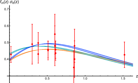
Figure 3: $z$ versus $f_{\rm m}{}(z)\sigma_{8}(z)$ for the three models: our model (blue), the Planck $\Lambda$CDM model (green) and the late time $\Lambda$CDM model (orange). Data points are from table 2 in the Appendix and the widths of the curves correspond to $1\sigma$ coming from the fits.

3 Discussion

The purpose of this article is to show that our modified Friedmann equation not only resolves the $H_{0}$ tension but also produces a function $H(z)$ which is consistent with the measured large scale structures of the Universe. We have shown that this is the case for the angular diameter distance defined by eq. (2), as well as for $f_{\rm m}(z)\sigma_{8}(z)$ defined by (14) and (18). Finally, our value of $S_{8}$, defined by (21) and given by (23), agrees with late time estimates, but has a tension with the value calculated from the Planck data by using the $\Lambda$CDM model. Our value, like the Planck value, is also calculated, based on physics identical to the CMB physics before $t_{\rm LS}$. The reason our $S_{8}$ value differs from the Planck value of $S_{8}$ is that our value of $\Omega_{\rm{m},0}=0.269$ while the Planck value is $\Omega_{\rm{m},0}=0.317$. The Planck value of $\Omega_{\rm{m},0}H_{0}^{2}$ is entirely determined by physics before $t_{\rm LS}$ since we have

$$\frac{\Omega_{\rm m}(t_{\rm LS})\big{(}H(t_{\rm LS})\big{)}^{{}2}}{\big{(}1+z(t_{\rm LS})\big{)}^{{}3}}\,=\,\Omega_{\rm m}(t_{0})\big{(}H(t_{0})\big{)}^{{}2}\,=\,\Omega_{{\rm m},0}H_{0}^{2}.$$ (24)

Our model will also satisfy eq. (24) and since our value of $H(t_{\rm LS})$ by assumption agrees with the Planck value at $z(t_{\rm LS})$ we will have the same value of $\Omega_{{\rm m},0}H_{0}^{2}$. However, by construction we have a larger value for $H_{0}$ than Planck collaboration since we used the $H_{0}$ measured at late time to determine our value of the constant $B$. Consequently we have a lower value of $\Omega_{{\rm m},0}$. $\Lambda$CDM with $\Lambda_{\rm SC}$ has the problem in the angular diameter distance.

This is possible because our late time cosmology is governed by our baby universe $B$-term and not by the cosmological constant. As already mentioned there are many suggestions of modification of the late time cosmology which produce more or less the same results as we have reported here for our model. However, many of these models are entirely phenomenological in nature, like using a spline interpolation of the measured function $H(z)$ for small $z$, or modifying the equation of state by hand without too much physical motivation. In this sense we feel that our model is special. It has just one parameter, denoted $B$ (much like the $\Lambda$CDM model), the origin of which goes back to the very early universe where it is related to the creation of baby universes. In this sense it relates the very origin of the Universe to its late destiny (the exponential expansion of the Universe at a rate proportional to $\sqrt[3]{B}$), and the presence of the parameter $B$ and the modified Friedmann equation is motivated by a physics model of the Universe. Admittedly, as already mentioned, we cannot presently solve our underlying model in detail and calculate $B$ and then follow the evolution of the universe from the very beginning of time (which in our model of the Universe is related to the breaking of an underlying $W_{3}$ symmetry [4]) to the present time, but that is work in progress….

Acknowledgments

YW acknowledges the support from JSPS KAKENHI Grant Number JP18K03612 and thanks A. Hosoya for discussions.

Appendix

Table 1: Baryon Acoustic Oscillation

$~{}~{}z$	$~{}~{}~{}r_{\rm s}/D_{\rm V}$	$~{}~{}~{}D_{\rm V}/r_{\rm s}$	Survey	ArXiv Reference
$0.106$	$0.336\pm 0.015$		6dFGS	1108.2635
$0.20$	$0.1980\pm 0.0058$		SDSS	0705.3323
$0.275$	$0.1390\pm 0.0037$		SDSS	0907.1660
$0.35$	$0.1097\pm 0.0036$		SDSS	1108.2635
$0.44$	$0.0916\pm 0.0071$		WiggleZ	1108.2635
$0.60$	$0.0702\pm 0.0032$		WiggleZ	1108.2635
$0.60$	$0.0726\pm 0.0034$		WiggleZ	1108.2635
$0.73$	$0.0592\pm 0.0032$		WiggleZ	1108.2635
$0.57$		$13.67\pm 0.22$	SDSS	1203.6594
$0.32$		$8.4673\pm 0.1675$	SDSS	1312.4877
$0.57$		$13.7728\pm 0.1340$	SDSS	1312.4877
$0.32$		$8.59386\pm 0.09474$	SDSS	1607.03155
$0.57$		$13.7569\pm 0.14210$	SDSS	1607.03155
$2.34$		$31.2409\pm 1.08716$	SDSS	1404.1801
$2.36$		$30.3548\pm 1.08678$	SDSS	1311.1767
$1.52$		$26.8\pm 1.1$	SDSS	1801.03062
$0.698$		$16.26\pm 0.31$	SDSS	2007.08993
$0.85$		$18.59\pm 1.27$	SDSS	2007.09009

Table 2: Redshift-Space Distortion $f\sigma_{8}$

$~{}~{}z$	$~{}~{}~{}f\sigma_{8}$	Survey	ArXiv Reference
$0.02$	$0.428\pm 0.048$	6dFGS	1611.09862
$0.30$	$0.49\pm 0.12$	SDSS	1310.2820
$0.38$	$0.430\pm 0.054$	BOSS	1607.03148v2
$0.51$	$0.452\pm 0.057$	BOSS	1607.03148v2
$0.61$	$0.457\pm 0.052$	BOSS	1607.03148v2
$0.38$	$0.497\pm 0.063$	BOSS	1607.03155v1
$0.51$	$0.458\pm 0.050$	BOSS	1607.03155v1
$0.61$	$0.436\pm 0.043$	BOSS	1607.03155v1
$0.60$	$0.55\pm 0.12$	VIPERS	1612.05645v3
$0.86$	$0.40\pm 0.11$	VIPERS	1612.05645v3
$1.52$	$0.426\pm 0.077$	SDSS	1801.03062
$0.85$	$0.35\pm 0.10$		2007.09009
$0.60$	$0.48\pm 0.12$	VIPERS	1612.05647
$0.86$	$0.48\pm 0.10$	VIPERS	1612.05647

Table 3: $S_{8}$

$~{}~{}~{}~{}S_{8}$	Survey	ArXiv Reference
$0.784\pm 0.013$	DES	2110.10141
$0.759{{+0.024}\atop{-0.021}}$	KiDS-1000	2007.15633
$0.759{{+0.025}\atop{-0.023}}$	DES-Y3	2105.13543
$0.795{{+0.049}\atop{-0.042}}$	HSC-BOSS	2111.02419
$0.7781{{+0.0094}\atop{-0.0094}}$	KiDS-DES	2105.12108
$0.766{{+0.020}\atop{-0.014}}$	KiDS-1000	2007.15632
$0.776{{+0.017}\atop{-0.017}}$	DES-Y3	2105.13549
$0.751{{+0.039}\atop{-0.039}}$	BOSS DR12	2112.04515
$0.720{{+0.042}\atop{-0.042}}$	BOSS$+$eBOSS	2106.12580
$0.736{{+0.051}\atop{-0.051}}$	BOSS	2110.05530
$0.73{{+0.03}\atop{-0.03}}$	DELS	2111.09898
$0.784{{+0.015}\atop{-0.015}}$	unWISE	2105.03421
$0.78{{+0.04}\atop{-0.04}}$	KiDS-DR3	2012.12273

References

-
[1]
J. Ambjørn and Y. Watabiki,
“A modified Friedmann equation,”
Mod. Phys. Lett. A 32 (2017) no.40, 1750224, [arXiv:1709.06497 [gr-qc]]. -
[2]
J. Ambjorn and Y. Watabiki,
“Easing the Hubble constant tension,”
Mod. Phys. Lett. A 37 (2022) no.07, 2250041, [arXiv:2111.05087 [gr-qc]]. -
[3]
S. R. Coleman,
“Why There Is Nothing Rather Than Something: A Theory of the Cosmological Constant,” Nucl. Phys. B 310 (1988) 643. -
[4]
J. Ambjorn and Y. Watabiki,
“A model for emergence of space and time,”
Phys. Lett. B 749 (2015) 149, [arXiv:1505.04353 [hep-th]].
“Creating 3, 4, 6 and 10-dimensional spacetime from W3 symmetry,”
Phys. Lett. B 770 (2017) 252, [arXiv:1703.04402 [hep-th]].
“CDT and the Big Bang,”
Acta Phys. Polon. Supp. 10 (2017) 299, [arXiv:1704.02905 [hep-th]].
“Models of the Universe based on Jordan algebras,”
Nucl. Phys. B 955 (2020), 115044, [arXiv:2003.13527 [hep-th]]. -
[5]
R. E. Keeley, S. Joudaki, M. Kaplinghat and D. Kirkby,
“Implications of a transition in the dark energy equation of state for the and tensions,”
JCAP 12 (2019), 035, [arXiv:1905.10198 [astro-ph.CO]]. -
[6]
E. Di Valentino, L. A. Anchordoqui, Ö. Akarsu, Y. Ali-Haimoud, L. Amendola, N. Arendse, M. Asgari, M. Ballardini, S. Basilakos and E. Battistelli, et al.,
“Cosmology intertwined III: and ,
Astropart. Phys. 131 (2021), 102604, [arXiv:2008.11285 [astro-ph.CO]].
L. Heisenberg, H. Villarrubia-Rojo and J. Zosso,
“Can late-time extensions solve the and tensions?,”
arXiv:2202.01202 [astro-ph.CO] -
[7]
M. G. Dainotti, B. De Simone, T. Schiavone, G. Montani, E. Rinaldi and G. Lambiase,
“On the Hubble constant tension in the SNe Ia Pantheon sample,”
Astrophys. J. 912 (2021) no.2, 150, [arXiv:2103.02117 [astro-ph.CO]]. -
[8]
N. Aghanim et al. (Planck),
“Planck 2018 results. VI. Cosmological parameters,”
Astron. Astrophys. 641, A6 (2020), arXiv:1807.06209 [astro-ph.CO]. -
[9]
L. Perivolaropoulos and F. Skara,
“Challenges for CDM: An update,”
arXiv:2105.05208 [astro-ph.CO]. - [10] F. Niedermann and M. S. Sloth, “Resolving the Hubble tension with new early dark energy,” Phys. Rev. D 102 (2020) no.6, 063527 [arXiv:2006.06686 [astro-ph.CO]].
-
[11]
A. G. Riess, W. Yuan, L. M. Macri, D. Scolnic, D. Brout, S. Casertano, D. O. Jones, Y. Murakami, L. Breuval and T. G. Brink, et al.
“A Comprehensive Measurement of the Local Value of the Hubble Constant with 1 km/s/Mpc Uncertainty from the Hubble Space Telescope and the SH0ES Team,”
arXiv:2112.04510 [astro-ph.CO]. -
[12]
M. Gatti et al. [DES],
“Dark Energy Survey Year 3 results: cosmology with moments of weak lensing mass maps,” [arXiv:2110.10141 [astro-ph.CO]].
M. Asgari et al.,
“KiDS-1000 Cosmology: Cosmic shear constraints and comparison between two point statistics,” [arXiv:2007.15633 [astro-ph.CO]].
A. Amon et al.,
“Dark Energy Survey Year 3 Results: Cosmology from Cosmic Shear and Robustness to Data Calibration,” [arXiv:2105.13543 [astro-ph.CO]].
H. Miyatake et al.,
“Cosmological inference from the emulator based halo model II: Joint analysis of galaxy-galaxy weak lensing and galaxy clustering from HSC-Y1 and SDSS,” [arXiv:2111.02419 [astro-ph.CO]].
C. García-García, J. R. Zapatero, D. Alonso, E. Bellini, P. G. Ferreira, E. M. Mueller, A. Nicola and P. Ruiz-Lapuente,
“The growth of density perturbations in the last 10 billion years from tomographic large-scale structure data,”
JCAP 10 (2021), 030, [arXiv:2105.12108 [astro-ph.CO]].
C. Heymans et al.,
“KiDS-1000 Cosmology: Multi-probe weak gravitational lensing and spectroscopic galaxy clustering constraints,” [arXiv:2007.15632 [astro-ph.CO]].
T.M.C. Abbott, et al.,
“Dark Energy Survey Year 3 Results: Cosmological Constraints from Galaxy Clustering and Weak Lensing,” [arXiv:2105.13549 [astro-ph.CO]].
O.H.E. Philcox et al.,
“The BOSS DR12 Full-Shape Cosmology: CDM Constraints from the Large-Scale Galaxy Power Spectrum and Bispectrum Monopole,” [arXiv:2112.04515 [astro-ph.CO]].
M.M. Ivanov,
“Cosmological constraints from the power spectrum of eBOSS emission line galaxies,” [arXiv:2106.12580 [astro-ph.CO]].
S. Chen et al.,
“A new analysis of galaxy 2-point functions in the BOSS survey, including full-shape information and post-reconstruction BAO,” [arXiv:2110.05530 [astro-ph.CO]].
M. White et al.,
“Cosmological constraints from the tomographic cross-correlation of DESI Luminous Red Galaxies and Planck CMB lensing,” [arXiv:2111.09898 [astro-ph.CO]].
A. Krolewski et al.,
“Cosmological constraints from unWISE and Planck CMB lensing tomography,” [arXiv:2105.03421 [astro-ph.CO]].
G.F. Lesci et al.,
“AMICO galaxy clusters in KiDS-DR3: cosmological constraints from counts and stacked weak-lensing,” [arXiv:2012.12273 [astro-ph.CO]].