New exact and analytic solutions in Weyl Integrable cosmology from Noether symmetry analysis

Abstract

We consider a cosmological model in a Friedmann–Lemaître–Robertson–Walker background space with an ideal gas defined in Weyl Integrable gravity. In the Einstein-Weyl theory a scalar field is introduced in a geometric way. Furthermore, the scalar field and the ideal gas interact in the gravitational Action Integral. Furthermore, we introduce a potential term for the scalar field potential and we show that the field equations admit a minisuperspace description. Noether’s theorem is applied for the constraint of the potential function and the corresponding conservation laws are constructed. Finally, we solve the Hamilton-Jacobi equation for the cosmological model and we derive a family of new solutions in Weyl Integrable cosmology. Some closed-form expressions for the Hubble function are presented.

I Introduction

Noether symmetry analysis is a powerful method for the construction of analytic solutions for dynamical systems which follow from a variational principle. Noether symmetries have been widely applied in gravitational physics and cosmology for the investigation of the integrability properties for the gravitational field equations ns1 ; ns2 ; ns3 ; ns4 ; ns5 ; ns6 ; ns7 . Additionally, Noether symmetries have been used as a geometric selection rule bas1 for the determination of the unknown parameters and functions in the gravitational Action Integral ,which have been introduced in order to explain the cosmological observations pl1 ; pl2 ; pl3 ; pl4 .

In large scales the universe is observed to be in an acceleration phase, which it is attributed to an matter source with negative pressure known as dark energy. For the physical origin of the dark energy various approaches have been proposed over the last decades in the literature, see for instance Ratra ; Barrow93 ; Copeland ; Overduin ; Basil ; Buda ; fq ; Ferraro ; faraonibook ; Ame10 ; rev ; ind . In the majority of the dark energy models new degrees of freedom are introduced in the gravitational Action integral such that the cosmological dynamics to change in a way in order the physical parameters describe the observable universe.

In this piece of work, we are interested in the construction of exact and analytic solutions for the cosmological field equations in Weyl Integrable Gravity (WIG) also known as Weyl Integrable Spacetime (WIST) salim96 ; ww1 ; ww2 ; ww3 ; ww4 ; ww5 . In Einstein theory of gravity the fundamental geometric object of the theory is the metric tensor. On the contrary, in Weyl-Einstein theory of gravity (in WIG) the fundamental geometric objects are the metric tensor and a scalar field. The novelty of the WIG is that the new degrees of freedom are introduced by the geometry of the physical space. Moreover, because of the geometric characteristics of the theory, the scalar field of WIG interacts in the Action Integral with the rest of the matter source of the universe. Cosmological models with interaction in the dark sector of the universe have been studied before theoretically and phenomenologically with very interesting results, see for instance in2 ; in4 ; in5 ; gr and references therein .

In our analysis we will show that when the matter source is described by an ideal gas, for instance by a radiation or a dust fluid source, the cosmological field equations in WIG admit a minisuperspace description and there exists a Lagrangian function which produces the field equations under variation. The Noether symmetry analysis is applied for the determination of the scalar field potential and the derivation of invariant functions and conservation laws. The plan of the paper is as follows.

In Section II we present the basic properties and definitions for the theory of variational symmetries, in particular we present the two theorems of E. Noether for the invariant transformations of the Action Integral. In Section III we define our model which is that of a spatially flat Friedmann–Lemaître–Robertson–Walker (FLRW) universe with an ideal gas as a matter source defined in WIG. Moreover we determine the minisuperspace for the cosmological model of our consideration and we write the point-like Lagrangian which describes the dynamical system.

Furthermore, in Section IV, we apply the Noether symmetry condition in order to constrain the free function of the cosmological model. We find that for a specific family of the exponential potential the field equations form a Hamiltonian integrable system where the Hamilton-Jacobi equation can be solved in a closed-form expression. Additionally, exact and analytic closed-form expressions which solve the field equations are presented. Finally, in Section V we summarize our results.

II Noether symmetry analysis

The symmetry analysis is a systematic mathematical method for the determination of invariant functions, similarity transformations and conservation laws, for the study of differential equations. Symmetry analysis was established by S. Lie at the end of the 19th century in a series of books lie1 ; lie2 ; lie3 . As it was shown by S. Lie, the transformation group which leaves invariant a given differential equation, or a system of differential equations, can be used to simplify the differential equation.

E. Noether in 1918 published a pioneer work noe18 for the determination of conservation laws of differential equations which follow from a variational principle. Inspired by the spirit of the work of S. Lie, Noether proved two novel theorems. The first theorem treats the invariance of the Action Integral under an infinitesimal transformation, while the second theorem provides a one-to-one correspondence for the symmetries of the Action Integral with conservation laws for the differential equations. Some similar studies on finite groups before the work of Noether, are that of Hamel h1 ; h2 , Herglotz h3 , Kneser h5 and Klein h6 , For a modern discussion on Noether’s work we refer the reader to the review nonle .

We continue our discussion of the case of Lagrangian functions which describe second-order differential equations and invariant transformations with point symmetries as generators.

Consider the infinitesimal transformation

$$t^{\prime} =t+\varepsilon\xi\left(t,x^{k}\right),$$ (1)

$$x^{\prime i} =x^{i}+\varepsilon\eta^{i}\left(t,x^{k}\right),$$ (2)

with generator the vector field

$$X=\frac{\partial t^{\prime}}{\partial\varepsilon}\partial_{t}+\frac{\partial x^{\prime i}}{\partial\varepsilon}\partial_{i}.$$

A dot indicates derivative with respect to the variable $t$. For the dynamical system of second-order ordinary differential equations $H\left(t,x^{k},\dot{x}^{k},\ddot{x}^{k}\right)$ which follows from the variation of the Lagrangian function $\mathcal{L}=\mathcal{L}\left(t,x^{k},\dot{x}^{k}\right)$, the vector field $X$ is a variational symmetry, i.e. Noether symmetry, if there exists a function $f$ such that the following condition is held

$$X^{\left[1\right]}\mathcal{L}+\mathcal{L}\dot{\xi}-\dot{f}=0~{}.$$ (3)

Hence, the Euler-Lagrangian equations, that is the dynamical system $H\left(t,x^{k},\dot{x}^{k},\ddot{x}^{k}\right)$ remain invariant under the action of the point transformation (1), (2). The symmetry condition (3) is known as Noether’s first theorem.

For a given Lagrangian function, equation (3) gives a monomial expression which is identical zero if the coefficients of the independent monomials are zero. From the latter a system of linear partial differential equations is defined.

The second Noether’s Theorem relates the existence of Noether symmetries to that of conservation laws. Indeed, if $X$ is the generator of the infinitesimal transformation (1), (2) which satisfies the symmetry condition (3) for a specific function$~{}f$, then the function

$$I\left(t,x^{k},\dot{x}^{k}\right)=\xi\left(\frac{\partial\mathcal{L}}{\partial\dot{x}^{k}}\dot{x}^{k}-\mathcal{L}\right)-\eta^{i}\frac{\partial\mathcal{L}}{\partial\dot{x}^{i}}+f,$$ (4)

is a conservation law for the dynamical system $H\left(t,x^{k},\dot{x}^{k},\ddot{x}^{k}\right)$, that is, $\dot{I}\left(t,x^{k},\dot{x}^{k}\right)=0.$

For a recent review of the application of Noether symmetries in gravitational theories we refer the reader to anrv while other applications of symmetries in gravitation physics can be found for instance in ap1 ; ap2 ; ap3 ; ap4

III Weyl Integrable Gravity

In WIG the geometry is defined by the metric tensor $g_{\mu\nu}$ and the scalar field $\phi$, in which $\tilde{g}_{\mu\nu}=\phi g_{\mu\nu}.$ The gravitational Action Integral is considered to be the

$$S_{W}=\int dx^{4}\sqrt{-g}\left(\tilde{R}+\xi\left(\tilde{\nabla}_{\nu}\left(\tilde{\nabla}_{\mu}\phi\right)\right)g^{\mu\nu}-V\left(\phi\right)+L_{m}\right),$$ (5)

in which $\tilde{R}$ is the Ricci scalar of the metric tensor $\tilde{g}_{\mu\nu}$, $\xi$ is the coupling constant of the scalar field $\phi$, $V\left(\phi\right)$ is the scalar field potential and $L_{m}$ is the Lagrangian component which attributes the matter source. In the following we shall assume that $L_{m}$ describes a perfect fluid.

The covariant derivative $\tilde{\nabla}_{\mu}$ is defined according to the Christoffel symbols of the metric tensor $\tilde{g}_{\mu\nu}$.

By definition, the following relations for the geometric elements of the conformal related metrics $\tilde{g}_{\mu\nu}$, $g_{\mu\nu}$ hold,

$$\tilde{\Gamma}_{\mu\nu}^{\kappa}\left(\tilde{g}\right)=\Gamma_{\mu\nu}^{\kappa}\left(g\right)-\phi_{,(\mu}\delta_{\nu)}^{\kappa}+\frac{1}{2}\phi^{,\kappa}g_{\mu\nu}.$$ (6)

$$\tilde{R}_{\mu\nu}\left(\tilde{g}\right) =R_{\mu\nu}\left(g\right)-\tilde{\nabla}_{\nu}\left(\tilde{\nabla}_{\mu}\phi\right)-\frac{1}{2}\left(\tilde{\nabla}_{\mu}\phi\right)\left(\tilde{\nabla}_{\nu}\phi\right)$$ (7)

$$-\frac{1}{2}g_{\mu\nu}\left(\frac{1}{\sqrt{-g}}\tilde{\nabla}_{\nu}\tilde{\nabla}_{\mu}\left(g^{\mu\nu}\sqrt{-g}\phi\right)-g^{\mu\nu}\left(\tilde{\nabla}_{\mu}\phi\right)\left(\tilde{\nabla}_{\nu}\phi\right)\right),$$

$$\tilde{R}\left(\tilde{g}\right)=R\left(g\right)-\frac{3}{\sqrt{-g}}\tilde{\nabla}_{\nu}\tilde{\nabla}_{\mu}\left(g^{\mu\nu}\sqrt{-g}\phi\right)+\frac{3}{2}\left(\tilde{\nabla}_{\mu}\phi\right)\left(\tilde{\nabla}_{\nu}\phi\right).$$ (8)

From the gravitational Action Integral (5) we derive the gravitational field equations of Weyl-Einstein theory salim96

$$\tilde{G}_{\mu\nu}+\tilde{\nabla}_{\nu}\left(\tilde{\nabla}_{\mu}\phi\right)-\left(2\xi-1\right)\left(\tilde{\nabla}_{\mu}\phi\right)\left(\tilde{\nabla}_{\nu}\phi\right)+\xi g_{\mu\nu}g^{\kappa\lambda}\left(\tilde{\nabla}_{\kappa}\phi\right)\left(\tilde{\nabla}_{\lambda}\phi\right)-V\left(\phi\right)g_{\mu\nu}=e^{-\frac{\phi}{2}}T_{\mu\nu}^{\left(m\right)},$$ (9)

where $\tilde{G}_{\mu\nu}\left(g\right)$ is the Weyl Einstein tensor and $T_{\mu\nu}^{\left(m\right)}=\left(\rho_{m}+p_{m}\right)u_{\mu}u_{\nu}+p_{m}g_{\mu\nu}$ is the energy momentum tensor which describes the matter source, $\rho_{m}$, $p_{m}$ are the energy density and pressure components respectively, while $u^{\mu}$ is the observer.

The field equation (9), with the use of (7) and (8) can be expressed in the equivalent form

$$G_{\mu\nu}-\lambda\left(\left(\nabla_{\mu}\phi\right)\left(\nabla_{\nu}\phi\right)-\frac{1}{2}g^{\mu\nu}g^{\kappa\lambda}\left(\nabla_{\kappa}\phi\right)\left(\nabla_{\lambda}\phi\right)\right)-V\left(\phi\right)g_{\mu\nu}=e^{-\frac{\phi}{2}}T_{\mu\nu}^{\left(m\right)},$$ (10)

in which the new parameter $\lambda$ is defined as $2\lambda\equiv 4\xi-3$. When $\lambda>0$, that is $\xi>\frac{3}{4}$, the scalar field is a real field, while when $\lambda<0$, i.e. $\xi<\frac{3}{4}$, the scalar field $\phi$ is a phantom field because its energy density can be negative.

The equations of motion for the scalar field and the fluid source are

$$-g^{\mu\nu}\nabla_{\nu}\nabla_{\mu}\phi+V\left(\phi\right)+\frac{1}{2\lambda}e^{-\frac{\phi}{2}}\rho_{m}=0$$ (11)

$$\left(\nabla_{\mu}e^{-\phi}\rho_{m}\right)u^{\mu}+e^{-\phi}\nabla_{\mu}u^{\mu}\left(\rho_{m}+p_{m}\right)=0.$$ (12)

From the latter expressions it is obvious that the coupling constant $\lambda$ determines the energy transfer and the nature of the interaction between the two different matter components; the scalar field $\phi$ and the perfect fluid $\rho_{m}$. For $\lambda>0$ energy transfers from the scalar field to the perfect fluid, while for $\lambda<0$ the inverse it holds. An interesting discussion on the nature of the coupling constant and its effects on the perturbations is presented in ss1 .

In the following we assume the perfect fluid to be an ideal gas, that is, $p_{m}=w_{m}\rho_{m}$, in which $w_{m}$ is a constant parameter. For $w_{m}=0$, the matter source $\rho_{m}$ describes a pressureless fluid source known as a dust fluid, while for $w_{m}=\frac{1}{3}$, the matter source $\rho_{m}$ describes a radiation fluid. For this analysis $w_{m}$ is bounded in the region $w_{m}\in\left(-1,1\right)$.

III.1 FLRW spacetime

According to the cosmological principle in large scales the universe is assumed to be isotropic and homogeneous described by the FLRW geometry. In addition, from the cosmological observations the spatial curvature is very small, thus the universe is described by the spatially flat FLRW spacetime with line element

$$ds^{2}=-N^{2}dt^{2}+a^{2}\left(t\right)\left(dr^{2}+r^{2}\left(d\theta^{2}+\sin^{2}\theta d\varphi^{2}\right)\right).$$ (13)

We assume the comoving observer $u_{\mu}=\frac{1}{N}\delta_{\mu}^{t}$, and $H=\frac{1}{N}\frac{\dot{a}}{a}$ is the Hubble constant. For the scalar field $\phi$ we assume that it inherits the symmetries of the background space, such that $\phi=\phi\left(t\right).$ Hence, the gravitational field equations are

$$3H^{2}-\frac{\lambda}{2N^{2}}\dot{\phi}^{2}-V\left(\phi\right)-e^{-\frac{\phi}{2}}\rho_{m}=0,$$ (14)

$$\dot{H}+H^{2}+\frac{1}{6}e^{-\frac{\phi}{2}}\left(\rho_{m}+3p_{m}\right)+\frac{1}{3}\left(\frac{\lambda}{N^{2}}\dot{\phi}^{2}-V\left(\phi\right)\right)=0,$$ (15)

$$\ddot{\phi}+3H\dot{\phi}+V\left(\phi\right)+\frac{1}{2\lambda}e^{-\frac{\phi}{2}}\rho_{m}=0,$$ (16)

$$\dot{\rho}_{m}+3NH\left(\rho_{m}+p_{m}\right)-\rho_{m}\dot{\phi}=0.$$ (17)

For an ideal gas, i.e. $p_{m}=w_{m}\rho_{m}\,$, equation (17) gives $\rho_{m}=\rho_{m0}a^{-3\left(w_{m}+1\right)}e^{\phi}$, where $\rho_{m0}$ is an integration constant which describes the energy density of the matter source at the present time.

If we replace $\rho_{m}$ in the field equations (14)-(16) it is easy to see that the rest of the field equations can be reproduced from the variation of the singular Lagrangian function

$$\mathcal{L}\left(N,a,\dot{a},\phi,\dot{\phi}\right)=\frac{1}{N}\left(-3a\dot{a}^{2}+\frac{\lambda}{2}a^{3}\dot{\phi}^{2}\right)-N\left(a^{3}V\left(\phi\right)+\rho_{m0}e^{\frac{\phi}{2}}a^{w_{m}}\right).$$ (18)

Lagrangian function (18) is a singular Lagrangian since $\frac{\partial\mathcal{L}}{\partial\dot{N}}=0.$ The second-order differential equations (15), (16) are the Euler-Lagrange equations with respect to the variables $a,$ and $\phi$, i.e. equations $\frac{d}{dt}\frac{\partial\mathcal{L}}{\partial\dot{a}}-\frac{\partial\mathcal{L}}{\partial a}=0$ ; $\frac{d}{dt}\frac{\partial\mathcal{L}}{\partial\dot{\phi}}-\frac{\partial\mathcal{L}}{\partial\phi}=0,$ respectively. Furthermore, equation (14) follows from the variation of (18) with respect to the lapse function $N,$ that is, $\frac{\partial\mathcal{L}}{\partial N}=0$. Equation (14) is nothing else than a constraint equation which can be seen as the Hamiltonian for the autonomous dynamical system (15), (16) if without loss of generality we consider $N\left(t\right)=N\left(a\left(t\right),\phi\left(t\right)\right)$.

In the latter case we apply the theory of symmetries of differential equations for the determination of conservation laws for the field equations. Specifically, we consider the application of Noether’s first theorem for the constraint of the scalar field potential $V\left(\phi\right)$, such that, the dynamical system described by the point-like Lagrangian (18) admits Noether point symmetries. Moreover, with the use of Noether’s second theorem conservation laws can be constructed.

IV Exact and analytic solutions from symmetry analysis

Without loss of generality we consider $N\left(t\right)=1$. Hence for the infinitesimal generator

$$X=\Xi\left(t,a,\phi\right)\partial_{t}+\eta^{a}\left(t,a,\phi\right)\partial_{a}+\eta^{\phi}\left(t,a,\phi\right)\partial_{\phi},$$ (19)

and the point-like Lagrangian (18); the symmetry condition (3) gives that for nonzero potential function $V\left(\phi\right)$, the Noether point symmetries for the cosmological model of our consideration WIG are, the vector field $X_{1}=\partial_{t}$ for arbitrary potential, while for

$$V\left(\phi\right)=V_{0}\exp\left(-\frac{\phi}{w_{m}-1}\right)~{},$$ (20)

there exists the additional Noether symmetry

$$X_{2}=2t\partial_{t}+\frac{2}{3}a\partial_{a}+4\left(w_{m}-1\right)\partial_{\phi}.$$ (21)

The exponential potential plays an important role in scalar field cosmology. In the absence of matter it provides a scaling solution which can describes the acceleration phase of the universe see for instance Copeland and references therein.

From Noether’s second theorem we are able to construct the conservation laws. For the vector field $X_{1}$ the conservation laws is the Hamiltonian function $\mathcal{H}=\left(\frac{\partial L}{\partial\dot{a}}\dot{a}+\frac{\partial L}{\partial\dot{\phi}}\dot{\phi}-\mathcal{L}\right)$, where from (14) it follows $\mathcal{H}=0$. Moreover, for the vector field $X_{2}$ we find the conservation law $I_{0}=2t\mathcal{H}-4a^{2}\dot{a}+4\lambda a^{3}\left(w_{m}-1\right)\dot{\phi}$, that is,

$$I_{0}=4a^{2}\dot{a}-4\lambda a^{3}\left(w_{m}-1\right)\dot{\phi}~{}.$$ (22)

We proceed with the application of the symmetry vector and of the conservation laws for the determination of exact and analytic solutions for the field equations.

IV.1 Exact solution

For the cosmological model with the scalar field potential (20), from the vector field $X_{2}$ we define the invariant functions $U_{1}=at^{-\frac{1}{3}}$, $U_{2}=\phi-2\left(w_{m}-1\right)\ln t$. We assume that the invariant functions are constant, that is,

$$a\left(t\right)=a_{0}t^{\frac{1}{3}}\text{, }\phi\left(t\right)=2\left(w_{m}-1\right)\ln t+\phi_{0}\text{~{}.}$$ (23)

where $a_{0}=U_{1}$ and $\phi_{0}=U_{2}$, in which without loss of generality we consider $\phi_{0}=0$.

By replacing in the field equations (14)-(17) it follows that (23) is an exact solution if and only if

$$V_{0} =\frac{1}{3}\frac{w_{m}-1}{w_{m}+1}\left(6\lambda-1-12w_{m}\lambda+6\lambda w_{m}^{2}\right),$$ (24)

$$\rho_{m0} =\frac{2}{3}\frac{a_{0}^{3\left(1+w_{m}\right)}}{3\left(1+w_{m}\right)}\left(6\lambda-1+12w_{m}\lambda+6\lambda w_{m}^{2}\right)~{}.$$ (25)

However, exact solution (23) describes a universe by a stiff fluid. The equation of the state parameter for the effective fluid is $w_{eff}=1$.

We continue with the determination of the analytic solution for the given model.

IV.2 Hamilton-Jacobi equation  

In order to solve the field equations we apply the Hamilton-Jacobi approach. We define the new variable $\psi=\phi-6\left(w_{m}-1\right)\ln a$, such that we write the field equations on the normal coordinates.

In the new variables the point-like Lagrangian (18) reads,

$$\mathcal{L}\left(a,\dot{a},\psi,\dot{\psi}\right)=3\left(1-6\left(w_{m}-1\right)^{2}\lambda\right)a\dot{a}^{2}-6\left(w_{m}-1\right)\lambda a^{2}\dot{a}\dot{\psi}-\frac{1}{2}\lambda a^{3}\dot{\psi}^{2}+a^{-3}\left(\rho_{m0}e^{\frac{\psi}{2}}+V_{0}e^{-\frac{\psi}{w_{m-1}}}\right).$$ (26)

We define the momentum $p_{a}=\frac{\partial\mathcal{L}}{\partial\dot{a}}$, $p_{\psi}=\frac{\partial\mathcal{L}}{\partial\dot{\psi}}$, that is,

$$p_{a} =6\left(1-6\left(w_{m}-1\right)^{2}\lambda\right)a\dot{a}-6\left(w_{m}-1\right)\lambda a^{2}\dot{\psi}~{},$$ (27)

$$p_{\psi} =-6\left(w_{m}-1\right)\lambda a^{2}\dot{a}-\lambda a^{3}\dot{\psi}~{},$$ (28)

from where it follows the Hamiltonian

$$\mathcal{H}\left(a,\psi,p_{a},p_{\psi}\right)\equiv\frac{1}{12a}p_{a}^{2}-\frac{w_{m}-1}{a^{2}}p_{a}p_{\psi}+\frac{\left(6\left(w_{m}-1\right)^{2}\lambda-1\right)}{2\lambda a^{3}}p_{\psi}^{2}-a^{-3}\left(\rho_{m0}e^{\frac{\psi}{2}}+V_{0}e^{-\frac{\psi}{w_{m-1}}}\right)=0.$$ (29)

In the new variables the conservation law $I_{0}$ reads

$$I_{0}=\frac{2}{3}ap_{a}.$$ (30)

In expression (29), we replace $p_{a}=\frac{\partial}{\partial a}S\left(a,\psi\right)$, $p_{\phi}=\frac{\partial}{\partial\psi}S\left(a,\psi\right)$, from where we derive the Hamilton-Jacobi equation

$$0 =\frac{1}{12a}\left(\frac{\partial}{\partial a}S\left(a,\psi\right)\right)^{2}-\frac{w_{m}-1}{a^{2}}\left(\frac{\partial}{\partial a}S\left(a,\psi\right)\right)\left(\frac{\partial}{\partial\psi}S\left(a,\psi\right)\right)$$ (31)

$$+\frac{\left(6\left(w_{m}-1\right)^{2}\lambda-1\right)}{2\lambda a^{3}}\left(\frac{\partial}{\partial\psi}S\left(a,\psi\right)\right)^{2}-a^{-3}\left(\rho_{m0}e^{\frac{\psi}{2}}+V_{0}e^{-\frac{\psi}{w_{m-1}}}\right)~{}.$$

Moreover, from the conservation law (30) we write the constraint equation

$$I_{0}=\frac{2}{3}a\frac{\partial}{\partial a}S\left(a,\psi\right).$$ (32)

By solving the Hamilton-Jacobi equation we determine the functional form for the Action $S\left(a,\psi\right)$, which can be used to write the field equations into an equivalent system of two first-order ordinary differential equations

$$\dot{a}=\frac{1-w_{m}}{a^{2}}\left(\frac{\partial S}{\partial\psi}\right)+\frac{1}{6a}\left(\frac{\partial S}{\partial a}\right)~{},$$ (33)

$$\dot{\psi}=\frac{\left(6\left(w_{m}-1\right)^{2}\lambda-1\right)}{\lambda a^{3}}\left(\frac{\partial S}{\partial\psi}\right)+\frac{1-w_{m}}{a^{2}}\left(\frac{\partial S}{\partial a}\right)~{}.$$ (34)

For a specific expression for the Action $S\left(a,\psi\right),$ the dynamical system (33), (34) describes the reduced system for the field equations provided by the Hamilton-Jacobi theory and the application of a transformation. Its solution can be used to write the $a$ and $\phi$ of the original system, as we shall see in the following lines.

Consequently, for $I_{0}=0$ and (32), the Action is given by the closed-form expression

$$S\left(a,\psi\right)=F\left(\psi\right)$$ (35)

with

$$\left(\frac{\partial F\left(\psi\right)}{\partial\psi}\right)^{2}=\frac{2\lambda\left(V_{0}+\rho_{m0}e^{\frac{w_{m}+1}{w_{m}-1}\psi}\right)}{e^{\frac{\psi}{w_{m}-1}}\left(6\lambda\left(w_{m}-1\right)^{2}-1\right)}~{}.$$ (36)

On the other hand for $I_{0}\neq 0$ and equation (32) the Action is

$$S\left(a,\psi\right)=\frac{3}{2}I_{0}\ln a+F\left(\psi\right),$$ (37)

with

$$\left(\frac{\partial F\left(\psi\right)}{\partial\psi}\right)=\frac{6I_{0}e^{\frac{\psi}{w_{m-1}}}\left(w_{m}-1\right)\lambda\pm\sqrt{\kappa\left(\Psi\right)}}{4e^{\frac{\psi}{w_{m}-1}}\left(6\lambda\left(w_{m}-1\right)^{2}-1\right)},$$ (38)

where

$$\kappa\left(\Psi\right)=2e^{\frac{\psi}{w_{m-1}}}\left(3e^{\frac{\psi}{w_{m-1}}}I_{0}^{2}+16V_{0}\left(6\lambda\left(w_{m}-1\right)^{2}-1\right)+16e^{\frac{1}{2}\frac{w_{m}+1}{w_{m}-1}\psi}\left(6\lambda\left(w_{m}-1\right)^{2}-1\right)\rho_{m0}\right).$$ (39)

Let us focus on the case with $I_{0}=0$ and for simplicity let us assume $w_{m}=0$. The Action $S\left(a,\psi\right)$ reads

$$\left(\frac{\partial F\left(\psi\right)}{\partial\psi}\right)^{2}=\frac{2\lambda\left(V_{0}e^{\psi}+\rho_{m0}e^{\frac{\psi}{2}}\right)}{6\lambda-1}\text{.}$$ (40)

Thus, the reduced system is

$$a^{2}\dot{a}=\pm\sqrt{\frac{2\lambda\left(V_{0}e^{\psi}+\rho_{m0}e^{\frac{\psi}{2}}\right)}{6\lambda-1}},$$ (41)

$$\dot{\psi}=\pm\frac{1}{a^{3}}\sqrt{\frac{2\left(6\lambda-1\right)}{\lambda}\left(V_{0}e^{\psi}+\rho_{m0}e^{\frac{\psi}{2}}\right)}.$$ (42)

Therefore, $\frac{d\psi}{da}=\frac{1}{a}\frac{\left(6\lambda-1\right)}{\lambda},$ or $\psi\left(a\right)=\frac{\left(6\lambda-1\right)}{\lambda}\ln a$. From the latter, it follows that the Hubble function is expressed by the closed-form expression

$$\left(H\left(a\right)\right)^{2}=\frac{2\lambda}{6\lambda-1}\left(V_{0}a^{-\frac{1}{\lambda}}+\rho_{m0}a^{-3-\frac{1}{2\lambda}}\right)\text{.}$$ (43)

This is an analytic solution which describes an equivalent system of two ideal gases non-interacting with constant equation of state parameters.

For the arbitrary parameter $w_{m}$, it follows $\frac{d\psi}{da}=\frac{1}{a}\frac{\left(6\lambda\left(w_{m}-1\right)^{2}-1\right)}{\lambda}$, in which the Hubble function is determined

$$\frac{H\left(a\right)^{2}}{H_{0}^{2}}=\bar{\Omega}_{1}a^{p_{1}}+\bar{\Omega}_{2}a^{p_{2}}.$$ (44)

with $\bar{\Omega}_{1}=\bar{\Omega}_{1}\left(\lambda,w_{m},V_{0}\right)$ , $\bar{\Omega}_{2}=\bar{\Omega}_{2}\left(\lambda,w_{m},\rho_{m0}\right)$ and indices $p_{1}=-6w_{m}+\frac{1}{w_{m}-1}\lambda$, $p_{2}=-3+3w_{m}\left(w_{m}-2\right)-\frac{1}{2\lambda}$.

The exact solution (44) describes a universe with two ideal gases $\left(\rho_{1},p_{1};p_{1}=w_{1}\rho_{1}\right)$ , $\left(\rho_{2},p_{2};p_{2}=w_{2}\rho_{2}\right)~{}$ with equation of state parameters $w_{1}\left(w_{m},\lambda\right)=-1-\frac{1}{3}p_{1}\left(w_{m},\lambda\right)$ and $w_{2}\left(w_{m},\lambda\right)=-1-\frac{1}{3}p_{2}\left(w_{m},\lambda\right)$. In Fig. 1 we present the contour plots for the effective equation of state parameters $w_{1}\left(w_{m},\lambda\right)$ and $w_{2}\left(w_{m},\lambda\right)~{}$ in the two-dimensional space of the free variables $\left(w_{m},\lambda\right)$. Such models have been widely studied before in the literature, see for instance jm01 and reference therein. Indeed, such exact solution provides physical parameters which can constrain some of the cosmological observations.

Indeed, for specific values of the free parameters $\left(w_{m},\lambda\right)$ we can recover various eras of the cosmological evolution. For the sets of parameters $\left(p_{1}=0,p_{2}=-3\right)$ or $\left(p_{1}=-3,p_{2}=0\right)$ the Hubble function for the $\Lambda$CDM is recovered and the scale factor is that of $a\left(t\right)=a_{0}\sinh^{\frac{2}{3}}\left(\frac{3}{2}H_{0}t\right)$. On the other hand, for $\left(p_{1}=0,p_{2}=-4\right)$ or $\left(p_{1}=-4,p_{2}=0\right)$ the solution with a cosmological constant and a radiation fluid is provided. Moreover, other dark energy models can be recovered where $w_{1}$ or $w_{2}$ take values lower than $-1$.

The deceleration parameter (44) can be easily derived as $q\left(a\right)=-1-\frac{d\ln H}{da}$ is derived. From the constraints $\left(p_{1}=0,p_{2}=-3\right)$ or $\left(p_{1}=-3,p_{2}=0\right)$ we calculate $\left(w_{m},\lambda\right)=\left(-3,84\right)$ and $\left(w_{m},\lambda\right)=\left(0,0\right)$. Thus in the present time, where $a=1$, the deceleration parameter is calculated to be a function of the form, $q\left(\bar{\Omega}_{1}\right)=3\bar{\Omega}_{1}-2$ and $q\left(\bar{\Omega}_{1}\right)=1-3\bar{\Omega}_{1}$. The present value of $q$ is considered to be $q\simeq 0.6~{}$jm01 , hence we derive $\bar{\Omega}_{1}\simeq 0.86$ or $\bar{\Omega}_{1}\simeq 0.13$. Which is clear that the specific gravitational model recovers some of the recent cosmological parameters.

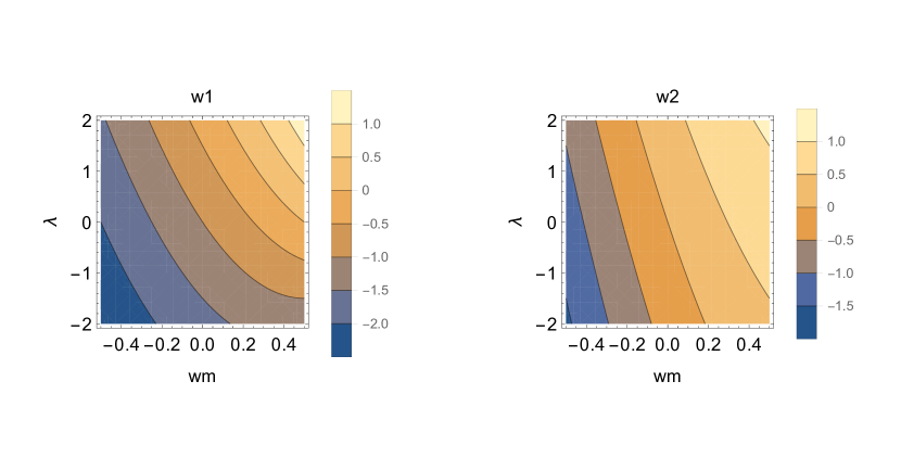
Figure 1: Contour plots for the effective equation of state parameters $w_{1}\left(w_{m},\lambda\right)=-1-\frac{1}{3}p_{1}\left(w_{m},\lambda\right)$ and $w_{2}\left(w_{m},\lambda\right)=-1-\frac{1}{3}p_{2}\left(w_{m},\lambda\right)$ in the two-dimensional space of the free variables $\left(w_{m},\lambda\right)$.

V Conclusions

In this study we applied the symmetry analysis of differential equations; specifically, the Noether symmetry conditions, for the constraint of the unknown parameters of a cosmological model with an ideal gas in WIG. A scalar field is introduced in the gravitational Action Integral as a result of Weyl geometry. The scalar field is minimally coupled with gravity but interacts with the matter source. The gravitational field equations admit a minisuperspace description. There exists a point-like Lagrangian function which produces the field equations under variation.

From Noether’s two theorems we were able to constrain the unknown potential function for the scalar field and we found that when it is exponential as it is given by expression (20) the field equations admit a second conservation law. Consequently the field equations form an integrable dynamical system and the Hamilton-Jacobi equation was explicitly solved. For a special value of the second conservation law we were able to write the Hubble function in a closed-form expression, where the cosmological solution consists of two ideal gases.

In the case of a general exponential potential $V\left(\phi\right)=V_{0}\exp\left(-\frac{\phi}{\kappa}\right)$. The closed-form solution follows

$$a\left(t\right)=a_{0}t^{\frac{2+\kappa}{3\left(1+w_{m}\right)}}~{},~{}\phi\left(t\right)=2\kappa\ln t~{},$$ (45)

with constraints for the free parameters of the model

$$V_{0} =-\frac{\kappa}{3\left(1+w_{m}\right)^{2}}\left(6\kappa\lambda\left(w_{m}^{2}-1\right)-2-\kappa\right)~{},$$ (46)

$$\rho_{m0} =-\frac{2a_{0}^{3\left(1+w_{m}\right)}}{3\left(1+w_{m}\right)^{2}}\left(6\kappa\lambda\left(w_{m}^{2}+1\right)-2-\kappa\right)~{}.$$ (47)

The latter solution is an exact solution of the model and not the general solution, because it has fewer free parameters than the degrees of freedom of the theory and it is valid only for a specific set of initial conditions for the original dynamical system. However, it is clear that cosmology in WIG in terms of the background space provides cosmological solutions of special interest.

At this point it is important to mention that the cosmological perturbations for a model with background equations similar with that of the present study were investigated before in ss1 . Thus similar results are expected and for our model.

The scale factor (45) describes a universe dominated by a perfect fluid with constant equation of state parameter, $w=\frac{2w_{m}-\lambda}{2+\kappa}$. For $w<-\frac{1}{3}$, the exact solution describes an accelerated universe, and this asymptotic solution can be used for the description of the early acceleration phase of the universe dw1 . This study provides for the first time analytic solutions for the Einstein-Weyl Integrable theory with a nonconstant potential function and nonzero matter component.  Analytic and exact solutions are essential for the study of a gravitational theory because we know that when a dynamical system is integrable there exist actual solutions which can describe the dynamics. The concept of the integrability in gravitational theories has been widely investigated by many scientists, see for instance int1 ; int2 ; int3 ; int4 .

From this analysis we conclude that the Noether symmetry analysis is a geometric criterion which provides physically accepted solutions in cosmological studies.

References

- (1) R. de Ritis, G. Marmo, G. Platania, C. Rubano, P. Scudellaro and C. Stornaiolo, New approach to find exact solutions for cosmological models with a scalar field, Phys. Rev. D 42, 1091 (1990)
- (2) K. Rosquist and C. Uggla, Killing tensors in two-dimensional space-times with applications to cosmology. J. Math. Phys. 32, 3412 (1991)
- (3) S. Capozziello, P. Martin-Moruno, and C. Rubano, Dark energy and dust matter phases from an exact f (R)-cosmology model, Phys. Lett. B 664, 12 (2008)
- (4) S. Cotsakis, P.G.L. Leach, C. Pantazi, Symmetries of homogeneous cosmologies. Gravit. Cosmol. 4, 314 (1998)
- (5) N. Dimakis, T. Christodoulakis, and P.A. Terzis, FLRW metric f (R) cosmology with a perfect fluid by generating integrals of motion. J. Geom. Phys. 77, 97 (2012)
- (6) J. A. Belinchon, T. Harko and M.K. Mak, Exact Scalar-Tensor Cosmological Solutions via Noether Symmetry. Astrophys. Space Sci. 361, 52 (2016)
- (7) S. Dutta and S. Chakraborty, A study of phantom scalar field cosmology using Lie and Noether symmetries, Int. J. Mod. Phys 25, 1650051 (2016)
- (8) S. Basilakos, M. Tsamparlis and A. Paliathanasis, Using the Noether symmetry approach to probe the nature of dark energy, Phys. Rev. D 86, 103512 (2011)
- (9) A. G. Riess, et al., Observational Evidence from Supernovae for an Accelerating Universe and a Cosmological Constant, Astron J. 116, 1009 (1998)
- (10) S. Perlmutter, et al., Measurements of and from 42 High-Redshift Supernovae, Astrophys. J. 517, 565 (1998)
- (11) P. A. R. Ade et al. [Planck Collaboration], Planck 2015 results. XIII. Cosmological parameters, Astron. Astrophys. 594, A13 (2016)
- (12) Planck Collaboration: N. Aghanim et al., Planck 2018 results. VI. Cosmological parameters, Astron. Astrophy. 641, A6 (2020)
- (13) B. Ratra and P.J.E. Peebles, Cosmological consequences of a rolling homogeneous scalar field, Phys. Rev. D 37, 3406 (1988)
- (14) J.D. Barrow and P. Saich, Scalar-field cosmologies, Class. Quant. Grav. 10, 279 (1993))
- (15) E.J. Copeland, M. Sami and S. Tsujikawa, Dynamics of dark energy, Int. J. Mod. Phys. D 15, 1753 (2006)
- (16) J.M. Overduin and F.I. Cooperstock, Evolution of the scale factor with a variable cosmological term, Phys. Rev. D 58, 043506 (1998)
- (17) S. Basilakos, M. Plionis and J. Sola, Hubble expansion and structure formation in time varying vacuum models, Phys. Rev. D 80, 083511 (2009)
- (18) H.A. Buchdahl, Non-Linear Lagrangians and Cosmological Theory, Mon. Not. Roy. Astron. Soc. 150, 1 (1970)
- (19) F.K. Anagnostopoulos, S. Basilakos and E.N. Saridakis, First evidence that non-metricity f(Q) gravity could challenge CDM, Phys. Lett. B 822, 136634 (2021)
- (20) R. Ferraro and F. Fiorini, Modified teleparallel gravity: Inflation without an inflaton, Phys. Rev. D 75, 084031 (2007)
- (21) V. Faraoni, Cosmology in Scalar-Tensor Gravity, Fundamental Theories of Physics vol. 139, (Kluwer Academic Press: Netherlands, 2004)
- (22) L. Amendola and S. Tsujikawa, Dark Energy Theory and Observations, (Cambridge University Press: Cambridge, 2010)
- (23) E. Di Valentino, O. Mena, S. Pan, L.Visinelli et al., In the realm of the Hubble tension—a review of solutions, Class. Quantum Grav. 38, 153001 (2021)
- (24) S. Nojiri, S.D. Odintsov and V.K. Oikonomou, Modified Gravity Theories on a Nutshell: Inflation, Bounce and Late-time Evolution, Phys. Rept. 692, 1 (2017)
- (25) J.M. Salim and S.L. Sautú, Gravitational theory in Weyl integrable spacetime, Class. Quantum Grav. 13, 353 (1996)
- (26) M. Yu Konstantinov and V.N. Melnikov, Integrable Weyl Geometry in Multidimensional Cosmology. Numerical Investigation, Int. J. Mod. Phys. D 4, 339 (1995)
- (27) C. Romero, J.B. Fonseca-Neto and M.L. Pucheu, General relativity and Weyl geometry, Class. Quantum Grav. 29, 155015 (2012)
- (28) A. Paliathanasis and G. Leon, Integrability and cosmological solutions in Einstein-æther-Weyl theory, EPJC 81, 255 (2021)
- (29) R. Gannouji, H. Nandan and N. Dadhich, FLRW cosmology in Weyl-Integrable Space-Time, JCAP 11, 051 (2021)
- (30) J. Miritzis, Acceleration in Weyl Integrable Spacetime, Int. J. Mod. Phys. D 22, 1350019 (2013)
- (31) W. Yang, S. Pan and A. Paliathanasis, Cosmological constraints on an exponential interaction in the dark sector, MNRAS 482, 1007 (2019)
- (32) W. Yang, A. Mukherjee, E. Di Valentino and S. Pan, Interacting dark energy with time varying equation of state and the H0 tension, Phys. Rev. D 98, 123527 (2018)
- (33) S. Pan and G.S. Sharov, A model with interaction of dark components and recent observational data, MNRAS 472, 4736 (2017)
- (34) G. Panotopoulos and I. Lopes, Interacting dark sector: Lagrangian formulation based on two canonical scalar fields, Phys. Rev. D 104, 083512 (2021)
- (35) S. Lie, Theorie der Transformationsgruppen I, Leipzig: B. G. Teubner (1888)
- (36) S. Lie, Theorie der Transformationsgruppen II, Leipzig: B. G. Teubner (1888)
- (37) S. Lie, Theorie der Transformationsgruppen III, Leipzig: B. G. Teubner (1888)
- (38) E. Noether, Invariante Variationsprobleme Königlich Gesellschaft der Wissenschaften Göttingen Nachrichten Mathematik-physik Klasse 2, 235-267 (1918)
- (39) Hamel G, Ueber die Grundlagen der Mechanik, Mathematische Annalen 66, 350-397 (1908)
- (40) G. Hamel, Ueber ein Prinzig der Befreiung bei Lagrange, Jahresbericht der Deutschen Mathematiker-Vereinigung 25, 60-65 (1917)
- (41) G. Herglotz, Über den vom Standpunkt des Relativitätsprinzips aus als starr zu bezeichnenden Körper, Annalen der Physik 336, 393-415 (1910)
- (42) A. Kneser, Kleinste Wirkung und Galileische Relativität Mathematische Zeitschrift 2, 326-349 (1918)
- (43) F. Klein, Königlich Gesellschaft der Wissenschaften Göttingen Nachrichten Mathematik-physik Klasse 2 (1918)
- (44) A.K. Halder, A. Paliathanasis and P.G.L. Leach, Noether’s Theorem and Symmetry, Symmetry 10, 744 (2018)
- (45) M. Tsamparlis and A. Paliathanasis, Symmetries of Differential Equations in Cosmology, Symmetry 10, 233 (2018)
- (46) T. Pailas, N. Dimakis, A. Paliathanasis, P.A. Terzis and T. Christodoulakis, Infinite dimensional symmetry groups of the Friedmann equations, Phys. Rev. D 102, 063524 (2020)
- (47) S. Dussault and V. Faraoni, A new symmetry of the spatially flat Einstein–Friedmann equations, EPJC 80, 1002 (2020)
- (48) S. Dussault, V. Faraoni and A. Giusti, Analogies between Logistic Equation and Relativistic Cosmology, Symmetry 13, 704 (2021)
- (49) G.Z. Abebe, S.D. Maharaj and K.S. Govinder, Gen. Rel. Grav. 46, 1733 (2014)
- (50) L. Amendola, Perturbations in a coupled scalar field cosmology, MNRAS 312, 521 (2000)
- (51) A. Paliathanasis, M. Tsamparlis, S. Basilakos and J.D. Barrow, Phys. Rev. D 93, 043528 (2016)
- (52) D. Wands, E.J. Copeland and A.R. Liddle, Ann. N.Y. Acad. Sci. 688, 647 (1993)
- (53) M. Francaviglia and J. Kijowski, Gen. Relativ. Grav. 12, 279 (1980)
- (54) E. Pozdeeva and S. Vernov, EPJ Web Conferences 125, 03008 (2016)
- (55) V.R. Ivanov and S.Y. Vernov, EPJC 81, 985 (2021)
- (56) V. R. Gavrilov, V. D. Ivashchuk and V. N. Melnikov, J. Math. Phys. 36, 5829 (1995)