The periodic zeta covariance function for Gaussian process regression

Abstract

I consider the Lerch-Hurwitz or periodic zeta function as covariance function of a periodic continuous-time stationary stochastic process. The function can be parametrized with a continuous index $\nu$ which regulates the continuity and differentiability properties of the process in a way completely analogous to the parameter $\nu$ of the Matérn class of covariance functions. This makes the periodic zeta a good companion to add a power-law prior spectrum seasonal component to a Matérn prior for Gaussian process regression. It is also a close relative of the circular Matérn covariance, and likewise can be used on spheres up to dimension three. Since this special function is not generally available in standard libraries, I explain in detail the numerical implementation.

1 Introduction

A Gaussian process, or Gaussian random field, is a distribution over an infinite dimensional space with Normal finite marginals; a finite-dimensional multivariate Normal is considered a specific case. Gaussian processes are used as distributions for statistical inference on functions with domain in time, space, or in general over quantities which have no fixed finite enumeration, that do not have a strongly constrained form. Applications range from geostatistics to optimization and machine learning. As general references, consider [17], [19], [16], and [7].

A Gaussian process is characterized by its covariance function, a two-point function that produces the entries of any marginal covariance matrix. In §6.7, [17] considers a covariance function with spectral mass over the lattice $\mathbf{j}\in\mathbb Z^{d}$ of the kind $(\alpha^{2}+|\mathbf{j}|^{2})^{-(\nu+d/2)}$, with parameters $\alpha,\nu>0$ (see also [18, eq. 4]), and proceeds to use it for inference with data on a regular square lattice using the discrete Fourier transform. In this article I calculate explicitly the covariance function for the $d=1$, $\alpha=0$ case, such that it can be used for any design layout and combined arbitrarily with other covariance functions, which amounts to evaluating the periodic zeta function $F(x,s)$ ([2, p. 257]).

This periodic covariance is one of the many generalizations of the Matérn class of covariance functions ([9, 406], [17, p. 31], [16, p. 84]), which include, to name a few examples, a non-stationary version ([14, 487]), a compactly supported version ([3, eq. 10]), and a smooth extension to spheres ([11, eq. 4]). In particular, [8] introduce an extension to spheres up to dimension three, naming it the circular Matérn covariance function, which amounts to considering the one-dimensional case of Stein’s periodic Matérn and evaluating it on the great arc distance. (See also [10] for calculations.)

[8] compare the circular Matérn with many other alternatives on a pair of examples. Although it performs well, on a practical note they recommend using the chordal Matérn, i.e., the usual Matérn evaluated on the embedding of the sphere, due to the complications in computing the circular Matérn: they give a closed form solution only for half-integer $\nu$, and no quickly converging approximation scheme. [15, 365], mention this as an open problem, and [1] propose as solution another covariance function with similar properties, the “F-family”, defined in terms of the Gauss hypergeometric function. Here I show how to compute exactly a function very similar to the circular Matérn, providing yet another alternative, albeit only up to the 3-sphere.

The layout of the article is as follows: Section 2 introduces the covariance function from first principles. Section 3 describes how to compute it efficiently and accurately. Finally, Section 4 concludes by mentioning some possible extensions.

2 The periodic zeta covariance function

Consider the standard Fourier series basis of functions

$$\{x\mapsto\cos(2\pi nx)\mid n=0,1,2,\ldots\}\cup\{x\mapsto\sin(2\pi nx)\mid n=1,2,3,\ldots\},$$ (1)

complete and orthonormal on the interval $x\in[0,1]$. Let $f(x)$ be a stochastic process defined in terms of the distribution of its coefficients in the Fourier basis, without the intercept term:

$$f(x)=\sum_{n=1}^{\infty}\big{(}c_{n}\cos(2\pi nx)+s_{n}\sin(2\pi nx)\big{)},$$ (2)

where the $c_{n}$ and $s_{n}$ are independently Normally distributed with variance

$$\operatorname{Var}[c_{n}]=\operatorname{Var}[s_{n}]=\frac{1}{n^{s}},$$ (3)

for some $s>1$. Since $f(x)$ is a linear combination of the coefficients, it is itself Normally distributed, i.e., a Gaussian process, with covariance function

$$\operatorname{Cov}[f(x_{1}),f(x_{2})] =\sum_{n=1}^{\infty}\big{(}\operatorname{Var}[c_{n}]\cos(2\pi nx_{1})\cos(2\pi nx_{2})+{}$$

$$\hphantom{{}=\sum_{n=1}^{\infty}\big{(}}\operatorname{Var}[s_{n}]\sin(2\pi nx_{1})\sin(2\pi nx_{2})\big{)}=$$

$$=\sum_{n=1}^{\infty}\frac{\cos(2\pi n(x_{1}-x_{2}))}{n^{s}}.$$ (4)

In this series we recognize the real part, evaluated at $x=x_{1}-x_{2}$, of the Lerch-Hurwitz or periodic zeta function

$$F(x,s)=E_{s}(x)=\sum_{n=1}^{\infty}\frac{e^{2\pi inx}}{n^{s}}.$$ (5)

The $F(x,s)$ notation is from the DLMF ([13, §25.13]), while $E_{s}(x)$ is from [4, §5.3]. To summarize, we have that a Gaussian process which is diagonal in the Fourier basis with period 1 with a power-law spectrum has the periodic zeta function as covariance function. The properties of this function are:

1. It depends only on the distance $|x_{1}-x_{2}|$, so the process is stationary.

2. The covariance function (and thus the process) is periodic with period 1.

3. $F(x,s)$ converges absolutely for all $x$ if $s>1$, and conditionally for non-integer $x$ if $s>0$.

4. $F(0,s)=\zeta(s)$, where $\zeta$ is Riemann’s zeta function.

5. $\partial_{x}F(x,s)=2\pi iF(x,s-1)$ for $s>1$ and non-integer $x$.

6. $\lim_{s\to\infty}F(x,s)=e^{2\pi ix}$.

For the covariance function, I introduce the notation

$$Z_{\nu}(x)=\frac{\Re F(x,1+2\nu)}{\zeta(1+2\nu)},\qquad\nu\geq 0,$$ (6)

with $x$ the difference $x_{1}-x_{2}$, where for $\nu=0$ I intend the limiting form of periodic white noise

$$Z_{0}(x)=\begin{cases}1&x\bmod 1=0,\\ 0&x\bmod 1\neq 0.\end{cases}$$ (7)

$Z_{\nu}$ may be called “periodic zeta covariance function.” Figure 1 shows it for some values of $\nu$. Due to property 4, it has unit variance. Due to 5, the derivative of the process has covariance function

$$\operatorname{Cov}[f^{\prime}(x_{1}),f^{\prime}(x_{2})] =\partial_{x_{1}}\partial_{x_{2}}Z_{\nu}(x_{1}-x_{2})=$$

$$=(2\pi)^{2}\frac{\zeta(1+2(\nu-1))}{\zeta(1+2\nu)}Z_{\nu-1}(x_{1}-x_{2}).$$ (8)

For $s<2$, $\partial_{x}\Re F(x,s)$ diverges for $x\to 0$, which means that, for $\nu<1/2$, $Z_{\nu}(x)$ has a cusp in $x=0$, indicating that the process is not mean-square Lipschitz-continuous. Together with Equation 8, this implies that a process with covariance function $Z_{\nu}(x)$ is $\lceil\nu\rceil-1$ times mean-square differentiable, and its highest order derivative is Lipschitz-continuous iff $\nu\bmod 1\geq 1/2$. See Appendix A for details.

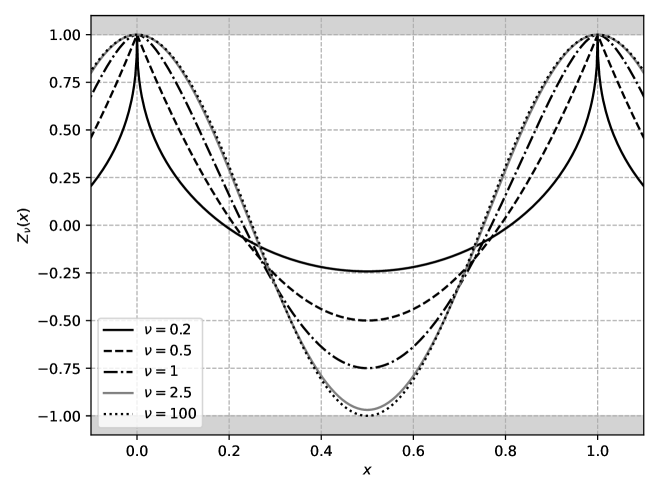
Figure 1: Plot of the covariance function $Z_{\nu}(x)$ from Equation 6 for some values of $\nu$. Due to property 6, for large $\nu$ it becomes a cosine.

Note that these properties w.r.t. $\nu$ are the same of the Matérn class of covariance functions ([16, p. 84], [17, p. 31])

$$M_{\nu}(x)=\frac{2}{\Gamma(\nu)}\left(\frac{r}{2}\right)^{\nu}K_{\nu}(r),\qquad r=\sqrt{2\nu}x,$$ (9)

including the white noise limit

$$\lim_{\nu\to 0^{+}}M_{\nu}(x)=\begin{cases}1&x=0,\\ 0&x\neq 0.\end{cases}$$ (10)

The circular Matérn covariance function ([8, eq. 7])

$$\psi_{\nu,\alpha}(\theta)\propto\sum_{k\in\mathbb Z}\frac{e^{ik\theta}}{(\alpha^{2}+k^{2})^{\nu+1/2}},\qquad\theta\in[0,\pi],$$ (11)

is equivalent to the periodic zeta in the limit $\alpha\to 0^{+}$ with the divergent $k=0$ intercept term removed and $\theta$ identified with $2\pi x$. Due to [5, corollary 4a], this is a positive definite function on the three-dimensional sphere $\mathbb S^{3}$ (and thus also $\mathbb S^{2}$) with $\theta$ the great arc distance. The same criterion also applies to the periodic zeta, in that $a/2^{s+1}+F(\theta/(2\pi),s)$ is a valid covariance function on $\mathbb S^{3}$ for $a\geq 1$ (see Appendix A).

What $Z_{\nu}$ lacks in comparison with $\psi_{\nu,\alpha}$ is a parameter regulating the correlation length like $\alpha$ does. To this end, consider the Lerch zeta function ([12, p. 17], [13, §25.14])

$$L(\lambda,\alpha,s)=\sum_{m=0}^{\infty}\frac{e^{2\pi i\lambda m}}{(m+\alpha)^{s}},$$ (12)

which counts as special case $F(x,s)=e^{2\pi ix}L(x,1,s)$. Thus I define a “Lerch covariance function”

$$Z_{\nu,\alpha}(x)=\frac{\Re e^{2\pi ix}L(x,\alpha,1+2\nu)}{\zeta(1+2\nu,\alpha)},\qquad Z_{\nu,1}(x)=Z_{\nu}(x),$$ (13)

which, like $Z_{\nu}$, has similar properties to the Matérn. Larger values of $\alpha$ produce a flatter spectrum head and thus shorten the correlation length. Although I do not treat in detail this extension, in Section 4 I give indications on how to compute it.

3 Numerical implementation

For large enough $s$, the series defining $F(x,s)$ (Equation 5) converges rapidly and can be summed directly. In practice this is convenient for $s\gtrsim 10$.

For small $s$, I make use of the relation with the Hurwitz zeta function ([13, eq. 25.13.2])

$$F(x,s)=\frac{\Gamma(1-s)}{(2\pi)^{1-s}}\left(e^{\pi i(1-s)/2}\zeta(1-s,x)+e^{-\pi i(1-s)/2}\zeta(1-s,1-x)\right).$$ (14)

This expression requires some attention because the factor $\Gamma(1-s)$ has a pole for integer $s$, canceled by a zero either due to the exponentials or to the symmetry property

$$\zeta(1-s,x)=(-1)^{s}\zeta(1-s,1-x),\qquad x\in[0,1],\quad s\in\mathbb N_{0},$$ (15)

derivable from [13, eq. 25.11.14] and the analogous symmetry of the Bernoulli polynomials. Thus, for $s$ close to an integer, these zeros must be computed accurately to all significant digits.

In the following, I discuss the calculation of the real part of $F(x,s)$. The procedure for the imaginary part is similar. I implemented this algorithm in the open-source software lsqfitgp and thoroughly measured its accuracy, which is 110 ULP at worst (relative to the maximum). See [4] for possible alternatives.

First, consider the real part of Equation 14

$$\Re F(x,s)=\frac{\Gamma(1-s)}{(2\pi)^{1-s}}\sin\left(\frac{\pi}{2}s\right)\big{(}\zeta(1-s,x)+\zeta(1-s,1-x)\big{)}.$$ (16)

For even $s$, the zero is in the sine term. The standard libraries can handle accurately the computation if $s$ is near zero. For other values, it is necessary to take the difference between $s$ and its nearest even integer, and change the sign of the sine appropriately.

For odd $s$, the zero is in the sum of Hurwitz zetas, thus it must be computed with full accuracy for almost odd $s$. I use the equations ([13, eq. 25.11.3 and 25.11.10])

$$\zeta(s,a) =\zeta(s,a+1)+a^{-s},$$ (17)

$$\zeta(s,a) =\sum_{n=0}^{\infty}\frac{(s)_{n}}{n!}\zeta(n+s)(1-a)^{n},$$ (18)

$$\qquad|1-a|<1,\quad(s)_{n}=s(s+1)\cdots(s+n-1),$$

to write the sum as

$$\zeta(1-s,x)+\zeta(1-s,1-x)=x^{s-1}+2\sum_{\text{even $n=0$}}^{\infty}\frac{(1-s)_{n}}{n!}\zeta(n+1-s)x^{n}.$$ (19)

Due to the symmetries of $F(x,s)$, I can take $x\in[0,1/2]$, and the term $(1-s)_{n}/n!$ is well bounded for $s<10$, thus the series in Equation 19 is geometrically convergent.

Consider how the series behaves as $s$ gets close to an odd integer $m$. $\zeta(s)=0$ for even negative $s$ ([13, eq. 25.6.4]), thus all the terms tend to zero for $n<m-1$. For $n>m-1$, the Pochhammer symbol $(1-s)_{n}$ contains the factor $(1-s+m-1)$, thus all those terms tend to zero too. The only nonzero term is the $n=m-1$ one, which for $s=m$ yields

$$\frac{n!}{n!}\zeta(0)x^{s-1}=-\frac{1}{2}x^{s-1},$$ (20)

thus canceling the external power in Equation 19.

The implications are that we have to compute accurately both the sum of the $(m-1)$-th term with $x^{s-1}$, and the zeta function near its zeroes. For the latter, use the reflection formula ([13, eq. 25.4.1])

$$\zeta(1-s)=2(2\pi)^{-s}\cos\left(\frac{\pi}{2}s\right)\Gamma(s)\zeta(s),$$ (21)

such that the zero is given by the cosine term. For the power, let $s=1+q+u$, with even integer $q$ and $|u|\leq 1/2$, and write the sum as

$$x^{q+u} +2\frac{(-q-u)_{q}}{q!}\zeta(-u)x^{q}=$$ (22)

$$=x^{q}\Bigg{(}e^{u\log x}-1+{}$$ (23)

$$\hphantom{{}=x^{q}\Bigg{(}}2\frac{\Gamma(1+q+u)}{\Gamma(1+q)\Gamma(1+u)}(\zeta(-u)-\zeta(0))+{}$$ (24)

$$\hphantom{{}=x^{q}\Bigg{(}}1-\frac{\Gamma(1+q+u)}{\Gamma(1+q)\Gamma(1+u)}\Bigg{)}.$$ (25)

Term (23) can be computed with the standard function expm1. The difference in (24) can be computed with the Taylor expansion around zero of the pole-free zeta $\tilde{\zeta}(s)=\zeta(s)-1/(s-1)$, yielding $1+\zeta(s)=\tilde{\zeta}(s)+s/(s-1)$. Finally, I write the difference in (25) as

$$\frac{\Gamma(1+q+u)}{\Gamma(1+q)\Gamma(1+u)}-1=e^{\log\Gamma(1+q+u)-\log\Gamma(1+q)-\log\Gamma(1+u)}-1,$$ (26)

where the Taylor series of $\log\Gamma(1+q+u)-\log\Gamma(1+q)$ and $\log\Gamma(1+u)$ can be generated with the generally available polygamma function $\psi_{n}$.

For $s$ exactly an integer, since the above algorithm is accurate arbitrarily close to an integer, just multiply $s$ by $1+\varepsilon$ before the computation, $\varepsilon$ being the ULP of 1.

Since the special functions $\Gamma$, $\zeta$ and $\psi_{n}$ need to be calculated on values depending only on $s$ and not $x$, this scheme scales well with the number of points the covariance function has to be evaluated at. The number of terms to be summed either in Equation 5 or Equation 19 is less than 50 for 53 bit floating point precision.

4 Conclusions

I have shown how to use in practice the covariance function of a power-law spectrum one-dimensional periodic process. In relation to the initial problem addressed by Stein (see Section 1), I left out two aspects: 1) the inverse correlation length $\alpha$, and 2) the multidimensional case.

To change the correlation length, consider the Lerch zeta function (Equation 12) with parameter $\alpha$ (note: not the same of Stein). For moderate integer $\alpha$, [13, eq. 25.14.4], allows to express the Lerch function in terms of the periodic zeta function described here. For more general algorithms, see [4]; algorithm 2 in particular ([6, eq. 9.555(2)]) gives a series similar to the one in Equation 19, likewise requiring care with pole canceling in the implementation, for $\alpha\in(0,1]$, which again can be extended to arbitrary but not too large $\alpha$ with repeated application of [6, eq. 9.551(1-2)].

To increase the dimensionality, I would need to efficiently evaluate the sum

$$\sum_{\begin{subarray}{c}\mathbf{n}\in\mathbb Z^{d}\\ \mathbf{n}\neq\mathbf{0}\end{subarray}}\frac{e^{2\pi i\mathbf{n}\cdot\mathbf{x}}}{|\mathbf{n}|^{s}},$$ (27)

which I am currently not able to do. An alternative of course is the separable sum or product of kernels over each axis.

A more practical aspect that I’ve neglected is the calculation of first and possibly second derivatives w.r.t. $\nu$, which would be useful for inference algorithms, from empirical Bayes to Markov chain Monte Carlo. I leave that to future work.

Appendix A Proofs

Smoothness of the process

I consider continuity and differentiability in the mean-square sense ([17, §2.4]). A process $f(x)$ is mean-square continuous if

$$\lim_{x\to y}E\big{[}(f(x)-f(y))^{2}\big{]}=0,$$ (28)

and mean-square differentiable if there exists $f^{\prime}(x)$ such that

$$\lim_{h\to 0}E\left[\left(\frac{f(x+h)-f(x)}{h}-f^{\prime}(x)\right)^{2}\right]=0.$$ (29)

These expected values translate into analogous expressions for the covariance function $K$. In particular, a stationary process is M.S. continuous iff $K$ is continuous in zero, and $m$ times M.S. differentiable iff $K$ is $2m$ times derivable in zero.

It follows that for $\nu>0$, $Z_{\nu}(x)$ (Equation 6) induces a M.S. continuous process. However, visual inspection of numerical simulations of the process shows that for $\nu<1/2$ it appears very discontinuous. To characterize this behavior, I consider Lipschitz continuity. I say that a process is M.S. Lipschitz-continuous if

$$\exists C\,\forall x,y:E\big{[}(f(x)-f(y))^{2}\big{]}\leq C(x-y)^{2}.$$ (30)

This property is violated if $\lim_{x\to 0^{+}}K_{\nu}^{\prime}(x)=-\infty$, since the ratio $(K_{\nu}(0)-K_{\nu}(x-y))/(x-y)$ becomes arbitrarily large as $x\to y$. To see that this is the case, consider that $\zeta(s,a)$ diverges for $a\to 0^{+}$ at fixed $s>0$ due to Equation 17, and that, for $0<\nu<1/2$, Equation 14 applies to $K_{\nu}^{\prime}(x)$ with $0<s<1$. This implies that $F(x,s)$ with $s\in(0,1)$ diverges for $x\to 0^{+}$, both in the real and imaginary part. But the imaginary part gives the derivative of $\Re F(x,s+1)\propto K_{\nu}(x)$.

The same continuity property can be proven about the Matérn class using [13, eq. 10.29.4 and 10.27.3].

Zero $\nu$ limit

Since $F(x,1)$ is finite for non-integer $x$ (property 3) and $\zeta(s)\sim 1/(s-1)$, $\lim_{\nu\to 0^{+}}Z_{\nu}(x)=0$ for $x\bmod 1\neq 0$.

A similar limit can be proven for the Matérn class $M_{\nu}(x)$ (Equation 9). The normalization is chosen to have $M_{\nu}(0)=1$, so it remains to show that $\lim_{\nu\to 0^{+}}M_{\nu}(x)=0$ for $x>0$. If it wasn’t for the $\sqrt{2\nu}$ rescaling, $x^{\nu}K_{\nu}(x)/\Gamma(\nu)$ would trivially converge to zero due to the finiteness of $K_{0}(x)$ and the pole of $\Gamma$. However, the $\sqrt{\nu}$ factor brings the evaluation point closer to zero, where $K_{\nu}$ diverges. Consider the series expansion ([13, eq. 10.27.4, 10.25.2])

$$K_{\nu}(2z)=\frac{\pi}{2}\sum_{k=0}^{\infty}\frac{1}{k!\sin(\pi\nu)}\left(\frac{z^{-\nu}}{\Gamma(1+k-\nu)}-\frac{z^{\nu}}{\Gamma(1+k+\nu)}\right)z^{2k}.$$ (31)

Replacing $z\mapsto\sqrt{\nu}x$, the leading term in $\nu$ is the first one, which goes like

$$(\sqrt{\nu}x)^{-\nu}-(\sqrt{\nu}x)^{\nu}=-2\sinh\left(\frac{1}{2}\nu\log\nu+\nu\log x\right)\sim\nu\log\nu\to 0.$$ (32)

The $\sin(\pi\nu)\sim\nu$ denominator is cancelled by the $\Gamma(\nu)\sim 1/\nu$ normalization.

Positive definiteness on the 3-sphere

[5, corollary 4a], gives the following necessary and sufficient condition for positive definiteness on $\mathbb S^{3}$ of a function $\psi$ defined in terms of the geodesic distance. Let

$$\psi(\theta)=\sum_{k=0}^{\infty}b_{n}\cos(n\theta),\qquad\theta\in[0,\pi],$$ (33)

be the Fourier series expansion of $\psi$. Then $\psi$ is a valid covariance function on $\mathbb S^{3}$, with $\theta$ the great circle distance, i.e., the angular length of the shorter arc connecting two points, or equivalently the arc along the intersection of a plane passing by the center and the two points with the sphere, if and only if

1. $b_{2}\leq 2b_{0}$, and

2. $b_{n+2}\leq b_{n}$ for $n\geq 1$.

The series of $F(x,s)$ (Equation 5) of course satisfies condition 2. To also have 1, it is necessary to add a constant term $b_{0}$ such that $2b_{0}\geq 2^{-s}$. This leads to the expression given at the end of Section 2.

References

- [1] A. Alegría, F. Cuevas-Pacheco, P. Diggle and E. Porcu “The F-family of covariance functions: A Matérn analogue for modeling random fields on spheres” In Spatial Statistics 43, 2021, pp. 100512 DOI: 10.1016/j.spasta.2021.100512
- [2] Tom M. Apostol “Introduction to Analytic Number Theory”, Undergraduate Texts in Mathematics Springer New York, NY, 1976 DOI: 10.1007/978-1-4757-5579-4
- [3] Moreno Bevilacqua, Christian Caamaño-Carrillo and Emilio Porcu “Unifying compactly supported and Matérn covariance functions in spatial statistics” In Journal of Multivariate Analysis 189, 2022, pp. 104949 DOI: 10.1016/j.jmva.2022.104949
- [4] R.E. Crandall “Unified algorithms for polylogarithm, L-series, and zeta variants” In Algorithmic Reflections: Selected Works PSI Press, 2012
- [5] Tilmann Gneiting “Strictly and non-strictly positive definite functions on spheres” In Bernoulli 19.4 Bernoulli Society for Mathematical StatisticsProbability, 2013, pp. 1327–1349 DOI: 10.3150/12-BEJSP06
- [6] I.. Gradshteyn and I.. Ryzhik “Table of Integrals, Series, and Products” Academic Press, Elsevier, 2014 URL: http://www.mathtable.com/gr
- [7] Robert B. Gramacy “Surrogates” ChapmanHall/CRC, 2020
- [8] Joseph Guinness and Montserrat Fuentes “Isotropic covariance functions on spheres: Some properties and modeling considerations” In Journal of Multivariate Analysis 143, 2016, pp. 143–152 DOI: 10.1016/j.jmva.2015.08.018
- [9] Mark S. Handcock and Michael L. Stein “A Bayesian Analysis of Kriging” In Technometrics 35.4 Taylor & Francis, 1993, pp. 403–410 DOI: 10.1080/00401706.1993.10485354
- [10] Chunfeng Huang and Ao Li “The Circular Matern Covariance Function and its Link to Markov Random Fields on the Circle” arXiv, 2022 DOI: 10.48550/ARXIV.2201.12856
- [11] Jaehong Jeong and Mikyoung Jun “A class of Matérn-like covariance functions for smooth processes on a sphere” In Spatial Statistics 11, 2015, pp. 1–18 DOI: 10.1016/j.spasta.2014.11.001
- [12] Antanas Laurincikas and Ramunas Garunkstis “The Lerch zeta-function” Springer Dordrecht, 2002 DOI: 10.1007/978-94-017-6401-8
- [13] F… Olver et al. “NIST Digital Library of Mathematical Functions”, Release 1.1.6 of 2022-06-30, 2022 URL: http://dlmf.nist.gov/
- [14] Christopher J. Paciorek and Mark J. Schervish “Spatial modelling using a new class of nonstationary covariance functions” In Environmetrics 17.5, 2006, pp. 483–506 DOI: 10.1002/env.785
- [15] Emilio Porcu, Alfredo Alegria and Reinhard Furrer “Modeling Temporally Evolving and Spatially Globally Dependent Data” In International Statistical Review 86.2, 2018, pp. 344–377 DOI: 10.1111/insr.12266
- [16] Carl Edward Rasmussen and Christopher K.. Williams “Gaussian Processes for Machine Learning”, 2006 URL: http://www.gaussianprocess.org/gpml/
- [17] Michael L. Stein “Interpolation of Spatial Data”, Springer Series in Statistics Springer New York, NY, 1999 DOI: 10.1007/978-1-4612-1494-6
- [18] Michael L. Stein “Space–Time Covariance Functions” In Journal of the American Statistical Association 100.469 Taylor & Francis, 2005, pp. 310–321 DOI: 10.1198/016214504000000854
- [19] Holger Wendland “Scattered Data Approximation”, Cambridge Monographs on Applied and Computational Mathematics Cambridge University Press, 2004 DOI: 10.1017/CBO9780511617539