Hybrid Cuckoo Search Algorithm for the Minimum Dominating Set Problem

Abstract.

The notions of dominating sets of graphs began almost 400 years ago with the game of chess, which sparked the analysis of dominating sets of graphs, at first relatively loosely until the beginnings of the 1960s, when the issue was given mathematical description. It’s among the most important problems in graph theory, as well as an NP-Complete problem that can’t be solved in polynomial time. As a result, we describe a new hybrid cuckoo search technique to tackle the MDS problem in this work. Cuckoo search is a well-known metaheuristic famed for its capacity for exploring a large area of the search space, making it useful for diversification. However, to enhance performance, we incorporated intensification techniques in addition to the genetic crossover operator in the suggested approach. The comparison of our method with the corresponding state-of-the-art techniques from the literature is presented in an exhaustive experimental test. The suggested algorithm outperforms the present state of the art, according to the obtained results.

Keywords: Minimum Dominating Set, Hybrid Cuckoo Search Algorithm, Genetic Algorithm.
2020 Mathematics Subject Classification. 05C69, 05Cxx, 90C59, 90C27.

1. Introduction

Given an undirected graph $G=(V,E)$, a subset $S$ of $V$ is named a dominating set of $G$ if each vertex $v\in V$ is either an element of $S$ or is adjacent to an element of $S$. Such subset is called a dominating set of $G$ and we say $S$ dominates $G$, or $G$ is dominated by $S$. The minimum cardinality of a dominating set in $G$ is denoted by $\gamma(G)$. If $S$ dominates $G$ such as $|S|=\gamma(G)$ then $S$ is called a Minimum Dominating Set, a MDS for short [1]. As an example, Figure 1 shows a subgraph of Twitter tweets with 85 vertices that spread specific 5G false news that is linked directly to the COVID-19 pandemic [2], with nodes denoting Twitter users and edges representing follower relationships, The MDS obtained by our approach is highlighted in red. The original status publisher is represented by the vertices of the dominating set, which are marked in red. If we assume the simplest scenario, followers, marked in blue, can not retweet and content can not spread out of followers, only 2 users could probably spread misinformation among the other 83 users.

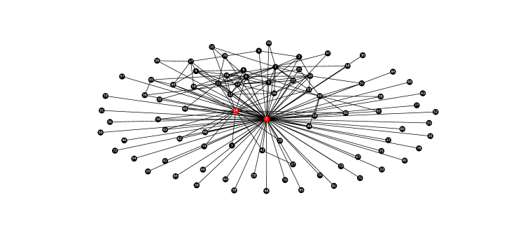
Figure 1. Representations of a real induced sub-graph from Twitter.

The minimum dominating sets and their variations, such as minimum connected dominating set and minimum weighted dominating set, have pervasive applications in a wide range of disciplines, besides Routing in ad hoc wireless networks [3, 4], Sensor Networks, and MANETs [5]. In addition, the MDS can be employed to determine the main subject sentences for document summary via sentence network design [6, 7]. Furthermore, the MDS may be used to model and investigate the positive impact in social networks [8, 9, 10, 11]. Moreover, controlling the spread of epidemics [12] also early diagnosis and control of epidemic spreadings in various areas of human society, such as Virus spread in computer systems, misinformation (as shown Figure 1), and content diffusion via social media [13]. MDS could be found in biological aspects such as interacting protein networks [14] and biological network analysis [15].

In this paper, we address the minimum dominating set problem by proposing a new Hybrid Cuckoo Search Algorithm, henceforth called HCSA-MDS, that combines the cuckoo search algorithm and the genetic crossover operator with intensification schemes as well as repairing and cleaning, to achieve effective exploration and exploitation.

1.1. Paper structure

The remainder of this paper is partitioned into many sections. In the Section 2 that follows, we present some linked works, including exact algorithms and heuristics, applied to solving the MDS problem. Section 3 goes into detail about the Cuckoo Search Algorithm. The Hybrid CSA algorithm is then presented and described in Section 4. Section 5, summarizes the results of the computation. The paper is finally concluded in the final Section 6.

2. Related works

The MDS problem is an NP-Hard combinatorial problem [16], it has been thoroughly investigated, using exact (exponential-time) techniques. Lately, several authors have independently developed exact algorithms that solve the MDS problem in a graph with $n$ vertices better than the trivial $\mathcal{O}(2^{n})$ time brute force methodology, which merely searches through all possible case subsets of $V$.

Initially, Fomin et al. proposed a nice exact algorithm based on the search space restriction that breaks the natural $2^{n}$ barrier for the MDS problem to an $\mathcal{O}(1.9379^{n})$ time algorithm on arbitrary graphs and lower time in some graph classes [17]. Then came various efforts on decreasing the time complexity of dominating sets, such as Ingo Schiermeyer who design an $\mathcal{O}(1.8899^{n})$ running time algorithm which is based on matching techniques to limit the search space [18]. After that, Grandoni decreased the running time to $\mathcal{O}(1.81^{n})$ [19]. Then there were the works of Fomin et al.[20], van Rooij and Bodlaender [21] and van Rooij et al. [22], which lowered the running time to around $\mathcal{O}(1.52^{n})$ more or less and in [23], van Rooij and Bodlaender reduced the running time to $\mathcal{O}(1.4969^{n})$. Currently, according to our information, the best exact algorithm for the MDS problem performs in $\mathcal{O}(1.4864^{n})$ time and polynomial space, and it is constructed through the measure and conquer approach [24] by Y. Iwata.

Unfortunately, the exact techniques that execute at an exponential scale are only possible for limited-size networks, severely limiting their effective uses. As a result, scientific researchers have mainly concentrated on stochastic computational heuristics and lately metaheuristics. Hence, many heuristic approaches have been adopted in the state of the art to handle the MDS problem, such as [25, 26, 27, 28]. Moreover, L. A. Sanchis [50] performed experimental research on different heuristic approaches in this perspective. He had thoroughly investigated many greedy methods for the MDS problem. After that, Ho et al.[49] presented ACO-TS, an improved Ant Colony Optimization metaheuristic that integrates a technique for stimulating the building of different solutions based on a concept adopted from genetic algorithms called tournament selection. Subsequently, in [31], Hedar and Ismail presented a hybrid genetic algorithm referred to as HGA-MDS that employs a local search which is characterized by three intensification techniques. Furthermore, in [32], also Hedar and Ismail suggested a SAMDS metaheuristic addressing the MDS problem by employing a Stochastic Local Search (SLS) algorithm for strengthening a solution by looking for a stronger one in its near area. The SLS is enhanced by using a simulated annealing process. Recently, Abed and Rais [33], introduced a hybrid population-based technique known as the Hybrid Bat Algorithm, which is rooted in microbat bio-sonar characteristics and simulated annealing. The fact that SA is efficient in exploitation and the bat algorithm has a high capacity for the exploration of large regions in the search space helps to ensure a good balance between intensification and diversification in the search methodology.

3. Cuckoo Search Algorithm

The Cuckoo Search Algorithm (CSA), based on fascinating breeding behavior of particular cuckoo species, such as brood parasitism, is one of the most recently developed metaheuristics [34].

Cuckoos are intriguing birds (see Figure 2), not just for their wonderful calls, but also for their aggressive breeding tactics. Some cuckoo species, such as the ani and guira, deposit their eggs in communal nests. However, they may remove other eggs to maximize the likelihood of their eggs hatching[36, 35].

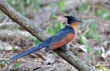
Figure 2. Chestnut-winged Cuckoo.

To describe Cuckoo Search for clarity, Yang and Deb use the following three idealized principles[37]:

1. One egg is laid by each cuckoo at a time, and it deposits it in a nest that is selected at random.

2. The best nests with the highest quality eggs (solutions with the highest fitness) will be passed on to future generations.

3. The number of host nests is fixed, and a host has a probability of discovering an alien egg of $P_{a}\in[0,1]$. In this scenario, the host bird can either discard the egg or leave the nest and create a new one at a different site.

A solution’s fitness can simply be proportional to the objective function’s value. A cuckoo egg signifies a new solution, and each egg in a nest indicates a solution. The goal is to replace the poor solutions in the nests with new and maybe improved solutions (cuckoos). This approach can be expanded to a more sophisticated scenario of several eggs representing a set of solutions in each nest. Therefore, we will take the simplest approach possible, with each nest containing only one egg. The CSA pseudo-code is shown in Algorithm 1 based on these criteria.

Algorithm 1 Cuckoo Search Algorithm: CSA

Input: Problem instance $S$
    Output: the best possible solution of $S$

1:  Initialize the population of $m$ host nests (solutions) $s=(s_{1},\ldots,s_{m})$;

2:  $t=0$;

3:  $maxGen=$ Maximum number of generations;

4:  while $t\leq maxGen$ do

5:     Select a cuckoo (say $x_{i}$) at random using Lévy flights and evaluate its fitness $f(x_{i})$;

6:     Choose one of $n$ (say $y_{i}$) nests at random;

7:     if $f(x_{i})>f(y_{i})$ then

8:        replace the old nest $x_{i}$ by the new one $y_{i}$

9:     end if

10:     A portion of the worst nests $p_{a}$ are removed and replaced with new ones;

11:     Sort the solutions and choose the best one;

12:     Refresh the current best solution;

13:     $t=t+1$;

14:  end while

After generating the initial population, CSA generates new solutions $x^{i+1}$ associated to each cuckoo $i$ in each iteration $t$ by a random walk via Lévy flight:

$$x_{i}^{t+1}=x_{i}^{t}+\alpha\oplus L\acute{e}vy(\lambda)$$ (1)

Several researchers have revealed that the flight behavior of many animals and insects exhibits typical Lévy flights characteristics [42, 39, 40, 41].

Lévy flights are a type of random walk named after the French mathematician Paul Lévy [42], in which $\alpha$ in the equation above denotes the step size which should correspond to the problem’s interests (most of the time $\alpha=1$) and the term product $\oplus$ denotes entrywise multiplications. The step lengths are selected from a probability distribution with a power law tail. Lévy distributions, or stable distributions, are the names given to these probability distributions.

$$L\acute{e}vy\sim u=l^{\lambda},$$ (2)

where $1<\lambda\leq 3$ and $l$ is the flight length [43].

The initial purpose of CSA and Lévy flights was to solve continuous optimization problems. Yang and Deb [37] show the outperform and the robustness of CSA over GA and PSO, because of its larger search space exploration capacity and fewer parameters to fine-tune than other algorithms. There is just one parameter $P_{a}$, separate from the population size $N$, CSA has been widely used and shown promising efficiency in a variety of optimization and computational intelligence applications[44].

On the other hand, Tein and Ramli suggested a discrete cuckoo search algorithm to handle nurse scheduling problems [46]. While Boumedine and Bouroubi proposed a discrete hybrid cuckoo search algorithm to solve the protein folding problem [47].

In this paper, we present a discrete hybrid CS-based method, called the Hybrid Cuckoo Search Algorithm for minimum dominating set (HCSA-MDS), to solve the MDS problem, which is one of the most difficult combinatorial optimization problems. The suggested discrete HCSA-MDS employs an adaptive Lévy flight for the MDS problem.

4. Hybrid CSA for the MDS problem

We describe our approach to tackling the MDS problem in the following section. Our algorithm takes as input a problem instance $G=(V,E)$, in which $G$ is an undirected, connected graph, $V$ is a set of vertices, and $E$ is a set of edges.

The HCSA-MDS combines the cuckoo search algorithm with the genetic crossover operator and the cleaning with repairing technique to exploit the solutions. While Lévy flights, with its ability to explore new regions in the search space, is a particularly useful strategy in the diversification phase. The goal of this hybridization is to establish a proper balance between search exploration and exploitation. The main structure is shown in Figure 3.

Figure 3. HCSA-MDS flowchart.

We first discuss the HCSA-MDS components before fully stating the HCSA-MDS algorithm 4.

4.1. Solution and population representation

The HCSA-MDS algorithm starts with a population $P$ that contains a set of $m$ nests (solutions), some of which are non-feasible. As a result, a $0-1$ vector with a dimension equal to the number of nodes in the graph $G=(V,E)$ represents a solution $x$ in $P$. The ith node in $G$ is part of the dominating set if the vector’s ith element has a value of 1. While the ith vector’s item has a value of 0, this indicates that a node is not part of the dominant set. Table 1 illustrates the binary representation of the solution of the Example 1 presented in Section 1.

1	2	3	$\cdots$	13	14	15	$\cdots$	85
0	1	0	$\cdots$	0	1	0	$\cdots$	0

Table 1. Binary representation of the best found MDS

4.2. A new cuckoo egg’s production using the crossover operator

The crossover operator is one of the genetic operators that applies to two parents (solutions) and then chooses at random any of the crossover points $p_{h}$ , $h\in\{0,1,...,n-1\}$ [30]. Two offspring (new solutions) are created by joining the parents at the crossover point for the next generation. However, for any solution from population $P$ that we consider the first parent, we randomly choose a second parent from the current population. Then, the one-point crossover operation is used to generate two offsprings. In the proposed algorithm, only the best offspring are chosen for the next stage, see the example in the following Table 2:

Parents	Binary representation		Offsprings	Binary representation
First	1010$\mid$10110	$\mathbf{\Rightarrow}$	First	1010$\mid$10010
Second	1111$\mid$10010		Second	1111$\mid$10110

Table 2. An illustrative example of a crossover operator with a single point-crossover.

In the previous example, the two offsprings are generated by combining the first and the second parents at the fourth position choosed randomly. Furthermore, in the example, the crossover generates two new solutions for which, in terms of minimum dominating set, the first one outperforms its parents and even its sibling.

4.3. Filtering procedure

For intensification, HCSA-MDS employs a filtering mechanism that cleans the MDS solutions by removing part of the redundant nodes. Cleaning attempts to limit the dominating set represented by the solution while maintaining its coverage [31]. The Filtering procedure is shown in Algorithm 2:

Algorithm 2 Filtering procedure

Input: Solution $S$.
     Output: Filtered solution.

1:  for each node $x$ in $S$ do

2:     if $x=1$ then

3:        Set $x=0$;

4:        compute the new fitness value of the solution $S$;

5:        if  the new fitness values is increased  then

6:           update the solution $S$ and set $x=0$;

7:        else

8:           reset $x=1$;

9:        end if

10:     end if

11:  end for

4.4. Reparation procedure

In this phase, we fix the solution $S$ that does not cover all nodes in this procedure. First we check whether the solution is not a dominating set, then the next vertex to be added to the set of dominators is always picked from vertices that are not in $S$ with the maximum degree. The reparation process stops when $S$ is a dominating set, as shown in Algorithm 3.

Algorithm 3 Reparation procedure

Input: Solution $S$.
     Output: Repaired solution.

1:  if there exist Non-covered nodes in the solution $S$ then

2:     Select a node $x$ with maximum degree in non-covered nodes set;

3:     Set $x=1$ and update the solution $S$;

4:     Remove $x$ from non-covered nodes and its neighbours;

5:  end if

4.5. Construction of new solution via Lévy flights

Fruit flies or Drosophila melanogaster, investigate their environment utilizing a sequence of straight flight pathways interrupted by a sharp $90\mathrm{°}$ rotation, resulting in an Lévy-flying-style discontinuous free exploration pattern on a large scale, according to Reynolds and Frye [39]. The basic features of Lévy flights can also be seen in studies of human behavior, such as foraging movement patterns that are used by human foragers [42].

Therefore, because of the step length features, Lévy flights are more efficient in exploring the search space. We link the step length (i.e., the length of the subset) with the value created by the Lévy flights to employ this technique for MDS. For example, if $s$ is an $n$-dimensional solution, we divide the interval $\left[0,1\right]$ into $m$ subintervals and define the step length($step_{length}$) as stated below:

$\theta$	$\left[0,\frac{1}{m}\right[$	$\left[\frac{1}{m},\frac{2}{m}\right[$	…	$\left[\frac{m-1}{m},1\right]$
$step_{length}$	$\left[1,\frac{\max_{l}}{m}\right[$	$\left[\frac{\max_{l}}{m},\frac{2\max_{l}}{m}\right[$	…	$\left[\frac{(m-1)\max_{l}}{m},\max_{l}\right]$

where $\theta$ is the Lévy flights value acquired and $\max_{l}=\frac{n}{h}$, $h\in\left\{1,2,3,\ldots,n\right\}$ is the maximum subset we are able to invert. Let $i$ be the length of the subset chosen randomly from the interval generated by Lévy’s flight value. Then, from the $n$-dimensional solution, we choose a random position between $1$ and $n-i$ from which the $i$-inversion begins.

4.6. HCSA-MDS Algorithm

Algorithm 4 HCSA-MDS

Input: A graph $G=(V,E)$.
     Output: Best Dominating Set.

1:  Initialization: Generate an initial population $P$ of $m$ feasible solutions,$S=(x_{i},\ldots,x_{m})$;

2:  $Gen=0$;

3:  while $Gen\leq Max$ (maximum number of generations) do

4:     $i=1$;

5:     while $i\leq m$ do

6:        Filter repaired solution to improve its quality;

7:        Select a random solution $x_{j}$ from $P$ as second parent;

8:        Produce a new cuckoo eggs $y_{j}$ using the crossover operator to the selected parents $x_{i}$ and $x_{j}$;

9:        if $f(y_{j})\geq f(x_{i})$ then

10:           Replace $x_{i}$ by the new produced solution $y_{j}$;

11:        end if

12:     end while

13:     The worst solutions are removed from $P$ and new ones are generated via Lévy flights proportional to $P_{a}\in\left[0,1\right]$;

14:     Rank the solutions from the best to the worst and find the best one;

15:     Update the global optimal solution;

16:  end while

5. Experimental results

HCSA-MDS effectiveness is evaluated against a collection of well-known efficient algorithms for the Minimum Dominating Set problem that has been reported in the literature. The rest of this section will be as follows. First, all benchmarks used are presented. Then, we compare the obtained results by the proposed algorithm with the state-of-the-art approaches.

To determine the relevance of the differences between the approaches results and HCSA-MDS Wilcoxon’s signed-rank test is used. It’s a nonparametric test method for analyzing matched-pair data. In addition, we employ Critical Difference (CD) diagrams that help to clarify things.

The Wilcoxon test is a powerful tool for detecting substantial variations between two algorithms’ performance, which will assist us in:

1. Determine which individual of a pair is ”greater than” i.e., determine the sign of any pair’s distinction.

2. Compare and contrast the differences.

The Wilcoxon signed-rank test is used for the evaluation of matched-pair statistics. The null hypothesis in the Wilcoxon’s signed-rank test is whether the probability distributions of the first and second data are equivalent, denoted $\mathcal{H}_{0}$ which means, the sum of the good ranks (the value of the first algorithm is greater than the second algorithm) is equal to the sum of the bad ranks (the value of the second algorithm is bigger than the first algorithm). However, if the sum of the good ranks differs from the sum of the bad ones, we reject $\mathcal{H}_{0}$ in favor of the alternative hypothesis, symbolized by $\mathcal{H}_{1}$, that the two algorithms differ [51].

When two scores achieved by any pair of algorithms are equal, which is signified by ties, all tied cases are removed from the analysis, reducing $N$, the number of matched pairs. This hypothesis can be evaluated using statistics based on intrapair differences and a null hypothesis refusal area equivalent to or less than $\alpha=0.05$ for a two-tailed test where the hypothesis is that the frequency for which the two signs appear will differ greatly.

Furthermore, Wilcoxon’s statistic uses these ranks to build a $Z$ score, which will be compared to a typical normal distribution to determine whether there are any variations between the algorithms. The $p$ value is then evaluated by comparing it to the $0.05$ significance level. We consider the null hypothesis if it is greater or equal to 0.05, for which the compared two algorithms do not differ. In contrast, if it is less than 0.05, we consider the alternative hypothesis, which is that the two algorithms differ and then one outperforms the other [52].

Critical difference (CD) diagrams, initially described in [53], were used to rank algorithms. They are a helpful tool for evaluating various algorithms. Before plotting any diagram, first use the non-parametric Friedman test, which analyzes each data set’s algorithms independently to determine the average ranks of algorithms to see whether there are any substantial differences. When the null hypothesis that all perform equally is well rejected, we conduct a post-hoc analysis. A Wilcoxon signed-rank test is used in the second phase to determine whether each pair of algorithms differs significantly [54]. We must use Holm’s approach to adapt Wilcoxon’s test because we are evaluating several hypotheses. Each considered algorithm is ranked on the horizontal axis in these diagram plots. The algorithm with the best performance receives a rank close to 1, the second receives a bigger rank, and so on. Strong horizontal bars connect the corresponding algorithms, for which we cannot differentiate from the Holm-adjusted Wilcoxon’s test, regarded as statistically equal.

5.1. Data Sets

The following two benchmarks are widely used in the literature for the MDS problem:

1. 42 random geometric graphs with upwards to 400 nodes, previously given in [32]. The authors used the generating instructions from [48, 49] to create the networks. Each network is created by inserting $n$ nodes, see column N^o of nodes in a $M\times M$ area at random according to the uniform distribution as shown in the column Area in Table 3. Several graph instances were generated for each network based on the range parameter listed in column Range in Table 3. They followed the instructions in [48] to guarantee that the graph formed a connected graph. Moreover, the number of graph instances per network was also included in the column N^o of instances.

   Network Id N^o of nodes ($n$) Range Area (A) N^o of instances N1${}_{A}^{n}$ 80 60-120 400$\times$400 7 N2${}_{A}^{n}$ 100 80-120 600$\times$600 5 N3${}_{A}^{n}$ 200 70-120 700$\times$700 6 N4${}_{A}^{n}$ 200 100-160 1000$\times$1000 7 N5${}_{A}^{n}$ 250 130-160 1500$\times$1500 4 N6${}_{A}^{n}$ 300 180-220 2000$\times$2000 5 N7${}_{A}^{n}$ 350 200-230 2500$\times$2500 4 N8${}_{A}^{n}$ 400 210-240 3000$\times$3000 4

   Table 3. First benshmark.

2. 21 graphs of 400 and 800 vertices, provided from [32]. In this benchmark set, the optimal dominating set is known. The authors employed the approach described in [50] to generate graphs with known domination numbers and provided densities henceforth denoted $\mathbf{N_{d,p}^{n}}$, where $n$ is the number of nodes, $d$ the domination number, and $p$ is the probability for edge creation. The detailed procedure is initially presented in [50].
   

   In this benchmark, we used two graphs of 400 and 800 vertices with different densities (0.1,0.3 and 0.5) and different domination numbers as presented in Table 4.

   Network $n$ $p$ $d$ N^o of graph instance $N_{d,0.1}^{400}$ $400$ $0.1$ $8,11,14,18,23$ $5$ $N_{d,0.3}^{400}$ $400$ $0.3$ $3,5,8,11,14$ $5$ $N_{d,0.5}^{400}$ $400$ $0.5$ $3,5,8,11$ $4$ $N_{d,0.1}^{800}$ $800$ $0.1$ $11,14,22$ $3$ $N_{d,0.3}^{800}$ $800$ $0.3$ $3,5$ $2$ $N_{d,0.5}^{800}$ $800$ $0.5$ $3,6$ $2$

   Table 4. Second benchmark.

Note that there are 63 graphs in both benchmark sets.

5.2. Tuning algorithm parameters

To conduct our experiment, we set the cuckoo search parameters respecting the common parameters used in the literature to address various optimization issues [37]. Table 5 shows the HCSA-MDS parameter values that produce the best performance. The first parameter $N$ is the population size, and the next parameter is maxGen, which represents the number of generations. However, the probability of the host bird discovering a cuckoo egg is $P_{a}$. Finally, the cuckoo’s step length parameters are $\gamma$ and $\alpha$.

Parameter	Value
$N$	$50$
$MaxGen$	$500$
$P_{a}$	$0.25$
$\gamma$	$3/2$
$\alpha$	$1$

Table 5. HCSA-MDS Parameters.

5.3. The numerical performance

Each benchmark was performed 10 times on every graph from the two literature data sets. However, for the second test case, we obtain the optimal dominant set from the first generation in all ten runs, except for four graphs that require more than 20 generations, so we generalize the number of generations up to 500 as stated in Section 5.2. Python was used to implement our HCSA-MDS algorithm. Furthermore, all testing was carried out on a system with 16 Gigabytes of RAM and a 2.6 GHz Intel Core i5 CPU. The suggested HCSA-MDS performance was evaluated using the two groups of data sets presented in Section 5.1. Table 6 shows the results of HCSA-MDS on 42 graph instances generated by the initial test cases. Tables 9 and 10 show the other HCSA-MDS performance on 21 graph instances generated by the second test scenarios.

5.3.1. Comparative analysis of HCSA-MDS against the state-of-art approaches on the first benchmark

We test the suggested HCSA-MDS on the first benchmark against HGA-MDS [31], SAMDS [32], and HBA [33] for the purpose of proving the performance of the HCSA-MDS approach check Table 6.

HGA-MDS SAMDS HBA HCSA-MDS Graph Id Range Best Avg. Std. Best Avg. Std. Best Avg. Std. Best Avg. Std. Worst N1${}_{400}^{80}$ 60 15 15.95 0.39 15 16.35 0.67 16 16.00 0 14 14.00 0 14^⋆ 70 13 14.00 0.73 12 14.40 1.14 13 13.30 0.48 11 11.00 0 11^⋆ 80 10 10.85 0.59 10 12.00 1.03 10 10.60 0.52 9 9.10 0.32 10^⋆ 90 8 8.40 0.50 8 9.60 1.27 9 9.60 0.52 8 8.00 0 8^⋆ 100 7 8,20 0.52 7 9.10 0.97 8 8.40 0.52 7 7.00 0 7^⋆ 110 6 6.05 0.22 6 7.55 0.69 6 6.90 0.32 6 6.00 0 6^⋆ 120 5 5.95 0.39 5 7.00 1.08 6 6.70 0.48 5 5.20 0.42 6 N2${}_{600}^{100}$ 80 19 19.55 0.85 18 20.55 1.23 19 19.00 0 15 15.90 0.32 16^⋆ 90 16 17.20 0.95 15 17.65 1.73 18 18.00 0 15 15.00 0 15^⋆ 100 14 14.85 0.49 13 14.95 1.05 14 14.40 0.52 13 13.20 0.42 14^⋆ 110 11 12.15 0.67 11 12.85 1.23 12 12.30 0.48 11 11.00 0 11^⋆ 120 10 10.15 0.37 9 12.00 1.49 11 11.00 0 9 9.00 0 9^⋆ N3${}_{700}^{200}$ 70 37 45.65 10.83 35 39.95 2.09 34 35.40 0.84 29 29.50 0.71 31^⋆ 80 31 33.05 1.32 29 33.50 1.73 28 28.20 0.42 25 25.50 0.97 28^⋆ 90 26 28.75 2.67 25 29,25 1.94 25 26.00 0.67 20 21.20 0.63 22^⋆ 100 21 24.70 4.94 20 24.20 1.70 21 21.80 0.42 18 19.00 0.47 20^⋆ 110 19 19.95 0.51 18 21.40 1.93 17 17.70 0.48 16 16.20 0.42 17^⋆ 120 17 17.30 0.47 15 19.55 1.43 15 16.20 0.79 14 14.00 0 14^⋆ N4${}_{1000}^{200}$ 100 39 45.25 5.57 38 41.35 1.87 36 36.70 0.48 29 29.70 0.82 31^⋆ 110 35 37.35 2.06 33 37.20 2.44 30 30.80 0.42 26 26.40 0.52 27^⋆ 120 27 28.90 1.77 26 30.10 1.45 26 26.30 0.48 23 23.10 0.32 24^⋆ 130 26 27.30 1.13 25 28.15 1.42 23 24.20 0.63 23 23.10 0.32 24 140 23 24.35 1.35 22 25.70 1.84 22 23.00 0.67 20 20.90 0.32 21^⋆ 150 21 21.45 0.76 20 23.55 1.43 19 20.30 0.82 18 18.10 0.32 19^⋆ 160 20 21.60 0.94 19 21.30 1.30 18 18.00 0 17 17.00 0 17^⋆ N5${}_{1500}^{250}$ 130 55 75.45 24.01 51 56.05 2.68 49 50.00 0.67 37 38.10 0.99 40^⋆ 140 48 59.75 12.78 46 48.65 1.35 42 42.60 0.70 40 41.10 0.57 42^⋆ 150 44 48.30 3.34 41 44.75 1.71 37 37.90. 0.32 37 37.60 0.52 38 160 38 41.65 3.42 37 40.90 1.92 31 32.60 1.71 30 30.40 0.52 31^⋆ N6${}_{2000}^{300}$ 180 54 61.20 6.64 47 52.35 2.41 44 45.70 0.95 43 43.10 0.32 44^⋆ 190 48 55.55 6.35 46 50.20 2.24 44 44.40 0.52 40 41.10 0.74 42^⋆ 200 41 47.90 5.07 40 45.25 2.55 41 41.10 0.32 36 36.40 0.52 37^⋆ 210 40 48.60 7.99 39 43.60 1.70 37 37.70 0.82 34 34.40 0.52 35^⋆ 220 36 39.90 4.34 36 40.65 1.90 33 34.10 0.57 31 31.80 0.79 33^⋆ N7${}_{2500}^{350}$ 200 67 93.45 23.58 61 66.35 2.13 58 58.90 0.32 47 48.10 0.57 49^⋆ 210 63 91.20 26.70 58 61.85 2.18 53 55.00 1.05 44 45.60 0.84 47^⋆ 220 55 76.85 30.55 49 55.05 2.31 51 51.80 0.63 44 44.60 0.52 45^⋆ 230 51 67.00 21.02 48 54.05 2.42 45 47.10 1.37 39 40.00 0.82 41^⋆ N8${}_{3000}^{400}$ 210 79 115.55 41.21 75 80.15 3.10 72 73.30 0.95 58 59.90 1.45 62^⋆ 220 77 110.45 39.76 73 79.25 3.18 70 71.00 0.82 56 56.40 0.52 57^⋆ 230 73 111.55 38.94 71 74.10 2.22 64 64.00 0 60 60.70 0.48 61^⋆ 240 70 103.15 32.02 63 68.80 2.98 58 59.30 0.67 55 56.60 0.70 57^⋆

Table 6. Performance comparison of various algorithms for the first benchmark sets.

HCSA-MDS performance is given for each instance in terms of:

1. The best solution is defined by the column denoted ”Best”, which defines the better solution identified by each approach, which is the minimum dominating set found in all runs for each graph instance.

2. Average: This indicator is given by the column labeled ”Avg.”, and it represents the mean of the finest solution values discovered in the individual runs of each graph instance.

3. The column labeled ”Std.” represents standard deviation, which is a statistic that measures the dispersion of the best solutions identified in runs.

4. The worst solution is defined by the column denoted ”Worst”, which is only for HCSA-MDS this measure represents the worst solution found in 10 runs for each graph instance.

5. The number of times we have gotten to the optimal solution in the column labeled ”Opt. Rea.” (see Table 9 and Table 10), which represents the number of runs on each graph for which the solution (domination number) was reached.

The following assessment can be drawn from the previous experiments (see Table 6):

• HCSA-MDS outperforms all the state-of-the-art solutions in terms of providing the best solution. Furthermore, HCSA-MDS can improve the best-known solution in 32 out of 42 graph instances and match the best-known solution for the rest of the 10 instances. For the larger graphs, the differences between HCSA-MDS and the other algorithms begin to grow. For example, in instances with 300, 350, and 400 vertices, HCSA-MDS provided better solutions in all graph instances with a substantial difference, as shown in Figure 5, which simulated the results of a best-solution comparison between HCSA-MDS and the other approaches. In addition, we used a critical difference diagram in Figure 4(b)4(a) to verify these results, showing that HCSA-MDS beats all other algorithms, followed by HBA, SAMDS, and HGA-MDS, which is the worst. In summarizing, we can assert that HCSA-MDS beats the state of the art in terms of solution quality by a large margin.

• Concerning the worst solution obtained over 10 runs, in 23 out of 42 graph instances, HCSA-MDS can outperform the currently best-known approaches. Furthermore, throughout the ten runs, HCSA-MDS does not produce worse solutions than those produced by the best solution in the state of the art. HCSA-MDS improves the best solution obtained by HBA in 29 instances and only matches HBA’s performance in 11 graphs. In only two cases did HBA find a solution that was better than HCSA-MDS’s worst solution. In 32 out of 42 graph instances, the HCSA-MDS worst solution is better than the best solution produced by SAMDS, and in 8 cases, it matches the best solution. In only two cases, the best solution provided by SAMDS is better than the worst solution by HCSA-MDS. In 35 instances, HCSA-MDS gave worst solutions that were better than HGA-MDS’s best solutions, 6 solutions were similar to the best solution, and in only one case, HGA outperformed HCSA-MDS in terms of worst solution. To recap, these details can be found in the Ranks Table 7. Table 8 displays Wilcoxon’s test statistics which show that there is a significant difference between HCSA-MDS and other approaches. Finally, Figure 4(b)4(b) shows the critical difference plot where HCSA-MDS exceeds the state of the art in terms of the worst solution when compared to the best solution yielded by literature approaches.

	HCSA-MDS			No
$\longrightarrow$	$>$	$<$	$=$	instances
HBA	29	2	11	42
SAMDS	32	2	8	42
HGA-MDS	35	1	6	42

Table 7. The ranks in summary.

Criteria	Algorithm	$Z$	Sig. ($p$ value)
Worst of HCSA-MDS	HCSA-MDS vs HBA	-4.671	0.000
VS	HCSA-MDS vs SAMDS	-4.918	0.000
Best of Others	HCSA-MDS vs HGA-MDS	-5.192	0.000

Table 8. Results of statistical significance between HCSA-MDS’s worst solutions and other approaches best solutions.

• The results of the standard deviation (column std.) in Table 6 clearly show that HCSA-MDS is more stable than HBA, as it gave stable dominating set values in 10 out of 42 instances, whereas HBA only provided stable dominating set values in 6 out of 42 instances. For both approaches, the standard deviation for the other cases is too near zero. SAMDS, on the other hand, outperforms HGA-MDS, which is the worst, especially in the densest graphs. This result is verified by the mean ranks of critical difference plots in Figure 4(b)4(c), where HCSA-MDS beats the other algorithms with statistical significance. Despite being ranked second, HBA’s stability is statistically equal to that of HCSA-MDS. Eventually, the HGA-MDS approach is the weakest in the analysis.

(a) Comparison of the best solutions (Best).

(b) HCSA-MDS worst solutions (Worst) compared to HBA,SAMDS, and HGA-MDS best solutions.

Figure 4. Critical Difference plots evaluating HCSA-MDS, HBA, SAMDS, and HGA-MDS for the first benchmark.

(c) Standard deviation (std.)

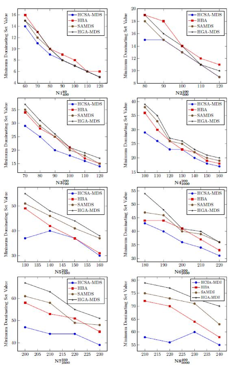
Figure 5. Best solution (Best) analysis of various approaches.

5.3.2. Numerical results for the HCSA-MDS and various approaches on the second benchmark

We discuss the effectiveness of the suggested HCSA-MDS on the second test case benchmark in this section. Our method’s results are evaluated against those of state-of-the-art algorithms. Hence, we compare HCSA-MDS against a variety of greedy algorithms from [50], where Sanshis L described and studied many greedy heuristics designated Greedy, GreedyRev, GreedyRan, GreedyVote, and GreedyVoteGr, which is an updated variant of GreedyVote. According to the evaluations, GreedyVoteGr beats other greedy heuristics when employing the local search process.

Similarly, we compare HCSA-MDS with the Hybrid Genetic Algorithm abbreviated HGA-MDS from [32], as well as Simulated Annealing (SAMDS) from the same paper [32] which shows better performance than HGA-MDS and the greedy heuristics.

The numerical values are presented in Tables 9 and 10. For each graph instance, the results of various approaches are presented in terms of the average solution (Avg.) obtained in 10 runs in each table. Three alternative graph densities are taken: from dense to sparse 0.5,0.3 and 0.1. For today’s state-of-the-art approaches, such benchmark sets are just very simple. Thus, we examine how many run out of 10, the Minimum Dominating Set was reached, which is represented in the column labeled ”Opt. Rea.”.

The experiments in Tables 9 and 10, show that HCSA-MDS is the highest performing algorithm with absolute distinctions in terms of average solution and reaching the optimal solution. Moreover,almost all instances 100% reaching the optimal in all 10 runs except two instances ($\mathbf{N_{0.3,3}^{400}}$,$\mathbf{N_{0.5,3}^{800}}$) optimal reached 8, 9 times respectively out of ten.

To determine the relevance of the differences between the approaches results and HCSA-MDS we used Wilcoxon’s signed-rank test. it only makes sense to consider only GreedyVoteGr, HGA-MDS, and SAMDS approaches, as they outperform the other greedy algorithms, moreover the results of the rest of the greedy methods are too similar.

The Test statistics presented in Table 11, show that there is a significant difference between HGA-MDS and the best performing algorithm in the Greedy series from [50], which is GreedyVoteGr in terms of both criteria. Furthermore, HGA-MDS could perform equally as well as SAMDS in terms of the mean of the solutions found, although SAMDS outperforms HGA-MDS in terms of the attainment rate of reaching the Minimum Dominating Set. Finally, HCSA-MDS outperforms SAMDS, HGA-MDS, and GreedyVoteGr since it is outperformed by HGA-MDS. To conclude, we can state that HCSA-MDS outperforms the state-of-the-art approaches in terms of robustness and stability.

Greedy GreedyRev GreedyRan GreedyVote GreedyVoteGr HGA-MDS SAMDS HCSA-MDS Opt. Opt. Opt. Opt. Opt. Opt. Opt. Opt. Graph d Avg. Rea. Avg. Rea. Avg. Rea. Avg. Rea. Avg. Rea. Avg. Rea. Avg. Rea. Avg. Rea. N${}_{0.1,d}^{400}$ 8 14.2 0 16.1 4 30.9 0 9.2 4 8 10 8 10 8 10 8 10 11 22.1 0 25.2 0 33.2 0 16.8 0 15.6 5 11.1 9 11.1 9 11 10 14 24 0 25.6 0 35.2 0 19 1 18.6 3 14.4 6 14.2 9 14 10 18 27.3 0 27.3 0 38.5 0 21.8 0 20.4 4 18.4 6 18 10 18 10 23 31.3 0 28.8 0 41.8 0 24.9 0 24.8 0 24.2 4 23 10 23 10 N${}_{0.3,d}^{400}$ 3 6.8 0 9.9 0 10.9 0 6.8 4 6 4 3 10 3.8 8 3.2 8 5 9 0 10.6 0 11.7 0 8.7 0 8.7 0 5.3 7 5.2 8 5 10 8 10.9 0 11.6 0 13.3 0 9.3 0 9.2 0 8.1 9 9 8 8 10 11 14 0 12.6 0 15.6 0 11.1 9 11 10 11 10 11 10 11 10 14 16.1 0 14.2 0 18.2 0 14 10 14 10 14 10 14 10 14 10 N${}_{0.5,d}^{400}$ 3 5 0 6.3 0 6.4 0 5 0 5 0 3.1 9 3.1 9 3 10 5 6 2 6.6 0 7 0 5.6 5 5.4 6 5.2 8 5.3 9 5 10 8 8.8 3 8.2 8 9 0 8.1 9 8 10 8 10 8 10 8 10 11 11.9 3 11 10 11.9 4 11 10 11 10 11 10 11 10 11 10

Table 9. Numerical results for various approaches as well as HCSA-MDS on $\mathbf{N_{p,d}^{400}}$.

Greedy GreedyRev GreedyRan GreedyVote GreedyVoteGr HGA-MDS SAMDS HCSA-MDS Opt. Opt. Opt. Opt. Opt. Opt. Opt. Opt. Graph d Avg. Rea. Avg. Rea. Avg. Rea. Avg. Rea. Avg. Rea. Avg. Rea. Avg. Rea. Avg. Rea. N${}_{0.1,d}^{800}$ 11 26.3 0 30.5 0 40.3 0 23.7 0 22.8 1 11.3 7 11.3 7 11 10 14 28.1 0 31.4 0 41.9 0 23.5 0 22.4 2 14 10 14 10 14 10 22 34.9 0 33.1 0 48.3 0 27.3 0 27.3 0 22.5 5 22 10 22 10 N${}_{0.3,d}^{800}$ 3 8.7 0 12.1 0 12.5 0 9 0 8.8 1 7.9 6 7.3 6 3 10 5 9.7 0 12.2 0 13.3 0 9.4 0 9.4 0 6.8 5 5 10 5 10 N${}_{0.5,d}^{800}$ 3 6 0 7.3 0 7 0 6 0 6 0 4.4 5 3.4 8 3.2 9 6 7.4 2 7.8 0 8.3 0 6.3 7 6.2 8 6.5 8 6 10 6 10

Table 10. Numerical results for various approaches as well as HCSA-MDS on $\mathbf{N_{p,d}^{800}}$.

Criteria	Algorithm	$Z$	Sig. ($p$ value)
Optimal Reached	HGA-MDS vs. GrVoteGr	-3.417	0.001
(Opt. Rea.)	SAMDS vs. HGA-MDS	-2.364	0.018
	HCSA-MDS vs. HGA-MDS	-3.136	0.002
	HCSA-MDS vs. SAMDS	-2.716	0.007
Averge	HGA-MDS vs. GrVoteGr	-3.413	0.001
(Avg.)	SAMDS vs. HGA-MDS	-1.609	1.08
	HCSA-MDS vs. HGA-MDS	-3.158	0.002
	HCSA-MDS vs. SAMDS	-2.814	0.005

Table 11. The Wilcoxon’s signed ranks test results for GreedyVoteGr, HGA-MDS, SAMDS, and HCSA-MDS.

6. Conclusion

In this paper, we addressed one of the fundamental NP-Hard problems in graph theory, which is the Minimum Dominating Set problem. We have proposed an effective Hybrid Cuckoo Search Algorithm abbreviated HCSA-MDS. HCSA-MDS outperforms the existing state-of-the-art techniques in terms of the best result obtained, according to an experimental evaluation on multiple benchmark sets. Furthermore, we tested the robustness of our proposed algorithm to state-of-the-art techniques utilizing the best, average, and even worst solutions, and found that HCSA-MDS outperformed other approaches.

HCSA-MDS, in our perspective, outperforms the state-of-art techniques, because it combines the cuckoo search algorithm, which uses Lévy flights to efficiently explore the search space, with multiple schemes for intensification and genetic crossover operator to exploit new solutions.

References

- [1] Haynes, Teresa W and Hedetniemi, Stephen and Slater, Peter, Fundamentals of domination in graphs, 2013, CRC press.
- [2] Schroeder, Daniel Thilo and Schaal, Ferdinand and Filkukova, Petra and Pogorelov, Konstantin and Langguth, Johannes WICO Graph: A Labeled Dataset of Twitter Subgraphs based on Conspiracy Theory and 5G-Corona Misinformation Tweets. ICAART (2), 257–266, 2021.
- [3] Dai, Fei and Wu, Jie, An extended localized algorithm for connected dominating set formation in ad hoc wireless networks, IEEE transactions on parallel and distributed systems, 15, 10, 908–920, 2004, IEEE
- [4] Wu, Jie and Li, Hailan, A dominating-set-based routing scheme in ad hoc wireless networks, Telecommunication Systems, 18, 1, 13–36, 2001, Springer.
- [5] Blum, Jeremy and Ding, Min and Thaeler, Andrew and Cheng, Xiuzhen, Connected dominating set in sensor networks and MANETs, bookHandbook of combinatorial optimization, 329–369, 2004, Springer.
- [6] Shen, Chao and Li, Tao, Multi-document summarization via the minimum dominating set, bookProceedings of the 23rd International Conference on Computational Linguistics (Coling 2010), 984–992, 2010.
- [7] Xu, Yi-Zhi and Zhou, Hai-Jun, Generalized minimum dominating set and application in automatic text summarization, bookJournal of Physics: Conference Series, 699, 1, 012014, 2016, IOP Publishing.
- [8] Dinh, Thang N and Shen, Yilin and Nguyen, Dung T and Thai, My T, On the approximability of positive influence dominating set in social networks, Journal of Combinatorial Optimization, 27, 3, 487–503, 2014, Springer
- [9] Daliri Khomami, Mohammad Mehdi and Rezvanian, Alireza and Bagherpour, Negin and Meybodi, Mohammad Reza, Minimum positive influence dominating set and its application in influence maximization: a learning automata approach, Applied Intelligence, 48, 3, 570–593, 2018, Springer.
- [10] Wang, Feng and Du, Hongwei and Camacho, Erika and Xu, Kuai and Lee, Wonjun and Shi, Yan and Shan, Shan, On positive influence dominating sets in social networks, Theoretical Computer Science, 412, 3, 265–269, 2011, Elsevier.
- [11] Wang, Guangyuan and Wang, Hua and Tao, Xiaohui and Zhang, Ji, Finding weighted positive influence dominating set to make impact to negatives: a study on online social networks in the new millennium, bookICTs and the millennium development goals, 67–80, 2014, Springer.
- [12] Takaguchi, Taro and Hasegawa, Takehisa and Yoshida, Yuichi, Suppressing epidemics on networks by exploiting observer nodes, Physical Review E, 90, 1, 012807, 2014, APS.
- [13] Zhao, Dawei and Xiao, Gaoxi and Wang, Zhen and Wang, Lianhai and Xu, Lijuan, Minimum dominating set of multiplex networks: definition, application, and identification, IEEE Transactions on Systems, Man, and Cybernetics: Systems, 51, 12, 7823–7837, 2020, IEEE.
- [14] Wuchty, Stefan, Controllability in protein interaction networks, Proceedings of the National Academy of Sciences, 111, 19, 7156–7160, 2014, National Acad Sciences.
- [15] Nacher, Jose C and Akutsu, Tatsuya, Minimum dominating set-based methods for analyzing biological networks, Methods, 102, 57–63, 2016, Elsevier.
- [16] Garey, Michael R and Johnson, David S, Computers and intractability, 174, 1979, freeman San Francisco.
- [17] Fomin, Fedor V and Kratsch, Dieter and Woeginger, Gerhard J, Exact (exponential) algorithms for the dominating set problem, bookInternational Workshop on Graph-Theoretic Concepts in Computer Science, 245–256, 2004, Springer.
- [18] Schiermeyer, Ingo, Efficiency in exponential time for domination-type problems, Discrete Applied Mathematics, 156, 17, 3291–3297, 2008, Elsevier.
- [19] Grandoni, Fabrizio, A note on the complexity of minimum dominating set, Journal of Discrete Algorithms, 4, 2, 209–214, 2006, Elsevier0.
- [20] Fomin, Fedor V and Grandoni, Fabrizio and Kratsch, Dieter, Some new techniques in design and analysis of exact (exponential) algorithms, Bull. EATCS, 87, 47–77, 2005.
- [21] Van Rooij, Johan MM and Bodlaender, Hans L, Design by measure and conquer, a faster exact algorithm for dominating set, arXiv preprint arXiv:0802.2827, 2008.
- [22] Van Rooij, Johan MM and Nederlof, Jesper and Dijk, Thomas C van, Inclusion/exclusion meets measure and conquer, bookEuropean Symposium on Algorithms, 554–565, 2009, Springer.
- [23] Exact algorithms for dominating set, Van Rooij, Johan MM and Bodlaender, Hans L, Discrete Applied Mathematics, 159, 17, 2147–2164, 2011, Elsevier.
- [24] Iwata, Yoichi, A faster algorithm for dominating set analyzed by the potential method, bookInternational Symposium on Parameterized and Exact Computation, 41–54, 2011, Springer.
- [25] Parekh, Abhay K, Analysis of a greedy heuristic for finding small dominating sets in graphs, Information processing letters, 39, 5, 237–240, 1991, Elsevier.
- [26] Wan, Peng-Jun and Alzoubi, Khaled M and Frieder, Ophir, A simple heuristic for minimum connected dominating set in graphs, International Journal of Foundations of Computer Science, 14, 02, 323–333, 2003, World Scientific.
- [27] Alkhalifah, Yaser and Wainwright, Roger L, A genetic algorithm applied to graph problems involving subsets of vertices, bookProceedings of the 2004 Congress on Evolutionary Computation (IEEE Cat. No. 04TH8753), 1, 303–308, 2004, IEEE.
- [28] Misra, Rajiv and Mandal, Chittaranjan, Minimum connected dominating set using a collaborative cover heuristic for ad hoc sensor networks, IEEE Transactions on parallel and distributed systems, 21, 3, 292–302, 2009, IEEE.
- [29] Sanchis, Laura A, Experimental analysis of heuristic algorithms for the dominating set problem, Algorithmica, 33, 1, 3–18, 2002, Springer.
- [30] Umbarkar, Anant J and Sheth, Pranali D, Crossover operators in genetic algorithms: a review., ICTACT journal on soft computing, 6, 1, 2015.
- [31] Hedar, Abdel-Rahman and Ismail, Rashad, Hybrid genetic algorithm for minimum dominating set problem, bookInternational conference on computational science and its applications, 457–467, 2010, Springer.
- [32] Hedar, Abdel-Rahman and Ismail, Rashad, Simulated annealing with stochastic local search for minimum dominating set problem, International Journal of Machine Learning and Cybernetics, 3, 2, 97–109, 2012, Springer.
- [33] Abed, Saad Adnan and Rais, Helmi Md, Hybrid bat algorithm for minimum dominating set problem, Journal of Intelligent & Fuzzy Systems, 33, 4, 2329–2339, 2017, IOS Press.
- [34] Cuckoo search algorithm: a metaheuristic approach to solve structural optimization problems, Gandomi, Amir Hossein and Yang, Xin-She and Alavi, Amir Hossein, Engineering with computers, 29, 1, 17–35, 2013, Springer.
- [35] Chestnut-winged Cuckoo (Clamator coromandus), Payne, RB and Kirwan, GM, Birds of the World, 1st ed.; del Hoyo, J., Elliott, A., Sargatal, J., Christie, DA, de Juana, E., Eds, 2020.
- [36] Payne, Robert B and Sorensen, Michael D, The cuckoos, 15, 2005, Oxford University Press.
- [37] Yang, Xin-She and Deb, Suash, Cuckoo search via Lévy flights, book2009 World congress on nature & biologically inspired computing (NaBIC), 210–214, 2009, Ieee.
- [38] Brown, Clifford T and Liebovitch, Larry S and Glendon, Rachel, Lévy flights in Dobe Ju/’hoansi foraging patterns, Human Ecology, 35, 1, 129–138, 2007, Springer.
- [39] Reynolds, Andy M and Frye, Mark A, Free-flight odor tracking in Drosophila is consistent with an optimal intermittent scale-free search, PloS one, 2, 4, e354, 2007, Public Library of Science San Francisco, USA.
- [40] Pavlyukevich, Ilya, Lévy flights, non-local search and simulated annealing, journal of computational physics, 226, 2, 1830–1844, 2007, Elsevier.
- [41] Pavlyukevich, Ilya, Cooling down Lévy flights, Journal of Physics A: Mathematical and Theoretical, 40, 41, 12299, 2007, IOP Publishing.
- [42] Brown, Clifford T and Liebovitch, Larry S and Glendon, Rachel, Lévy flights in Dobe Ju/’hoansi foraging patterns, Human Ecology, 35, 1, 129–138, 2007, Springer.
- [43] Viswanathan, Gandimohan M and Buldyrev, Sergey V and Havlin, Shlomo and Da Luz, MGE and Raposo, EP and Stanley, H Eugene, Optimizing the success of random searches, nature, 401, 6756, 911–914, 1999, Nature Publishing Group.
- [44] Yang, Xin-She and Deb, Suash, Cuckoo search: recent advances and applications, Neural Computing and applications, 24, 1, 169–174, 2014, Springer.
- [45] Walton, S and Hassan, O and Morgan, K and Brown, MR, Modified cuckoo search: a new gradient free optimisation algorithm, Chaos, Solitons & Fractals, 44, 9, 710–718, 2011, Elsevier.
- [46] Recent advancements of nurse scheduling models and a potential path, Lim, Huai Tein and Ramli, Razamin, 2010, Citeseer.
- [47] Boumedine, Nabil and Bouroubi, Sadek, Protein folding in 3D lattice HP model using a combining cuckoo search with the Hill-Climbing algorithms, Applied Soft Computing, 119, 108564, 2022, Elsevier.
- [48] Bettstetter, Christian, On the minimum node degree and connectivity of a wireless multihop network, bookProceedings of the 3rd ACM international symposium on Mobile ad hoc networking & computing, 80–91, 2002.
- [49] Ho, Chin Kuan and Singh, Yashwant Prasad and Ewe, Hong Tat, An enhanced ant colony optimization metaheuristic for the minimum dominating set problem, Applied Artificial Intelligence, 20, 10, 881–903, 2006, Taylor & Francis.
- [50] Experimental analysis of heuristic algorithms for the dominating set problem, Sanchis, Laura A, Algorithmica, 33, 1, 3–18, 2002, Springer.
- [51] Sheskin, David J, Handbook of parametric and nonparametric statistical procedures, 2003, Chapman and Hall/CRC.
- [52] Toothaker, Larry E, Book Review: Nonparametric Statistics for the Behavioral Sciences Sidney Siegel and N. John Castellan, Jr. New York: McGraw-Hill, 1988, 399 pp., Applied Psychological Measurement, 13, 2, 217–219, 1989, Sage Publications Sage CA: Thousand Oaks, CA.
- [53] Demšar, Janez, Statistical comparisons of classifiers over multiple data sets, The Journal of Machine learning research, 7, 1, 1–30, 2006.
- [54] Benavoli, Alessio and Corani, Giorgio and Mangili, Francesca, Should we really use post-hoc tests based on mean-ranks?, The Journal of Machine Learning Research, 17, 1, 152–161, 2016.