A mass transport approach to the optimization of adapted couplings of real valued random variables.

RΓ©mi Lassalle UniversitΓ© Paris 9 (Dauphine), PSL, Place du MarΓ©chal De Lattre De Tassigny, 75775 Paris Cedex 16, France lassalle@ceremade.dauphine.fr
Abstract.

In this work, we investigate an optimization problem over adapted couplings between pairs of real valued random variables, possibly describing random times. We relate those couplings to a specific class of causal transport plans between probabilities on the set of real numbers endowed with a filtration, for which their provide a specific representation, which is motivated by a precise characterization of the corresponding deterministic transport plans. From this, under mild hypothesis, the existence of a solution to the problem investigated here is obtained. Furthermore, several examples are provided, within this explicit framework.

Key words and phrases:
Stochastic analysis, optimal transport, optimization, filtrations.

Mathematics Subject Classification : 60H99 ;

1. Introduction

For the sake of clarity, in this work, the set 𝕋𝕋\mathbb{T} which within models encountered here may label times, will be the whole real line ℝℝ\mathbb{R}. We investigate the connections between adapted mass transport problems and optimization over fixed marginals couplings (X,Y,(Ξ©,π’œ,β„™))π‘‹π‘ŒΞ©π’œβ„™(X,Y,(\Omega,\mathcal{A},\mathbb{P})) of the specific form :

Definition 1.1.

Let X:Ω→ℝ:𝑋→ΩℝX:\Omega\to\mathbb{R} and Y:Ω→ℝ:π‘Œβ†’Ξ©β„Y:\Omega\to\mathbb{R} be two random variables defined on a same β„™βˆ’limit-fromβ„™\mathbb{P}- complete probability space (Ξ©,π’œ,β„™)Ξ©π’œβ„™(\Omega,\mathcal{A},\mathbb{P}). We say that (X,Y,(Ξ©,π’œ,β„™))π‘‹π‘ŒΞ©π’œβ„™(X,Y,(\Omega,\mathcal{A},\mathbb{P})) is an adapted coupling, if and only if, there exist two random variables Ο„:Ω→ℝ:πœβ†’Ξ©β„\tau:\Omega\to\mathbb{R}, and Z:Ω→ℝ:𝑍→ΩℝZ:\Omega\to\mathbb{R}, such that

Y=(X+Z)β€‹πŸ™{X≀τ}+Ο„β€‹πŸ™{X>Ο„},β„™βˆ’a.s.,formulae-sequenceπ‘Œπ‘‹π‘subscript1π‘‹πœπœsubscript1π‘‹πœβ„™π‘Žπ‘ Y=(X+Z)\mathds{1}_{\{X\leq\tau\}}+\tau\mathds{1}_{\{X>\tau\}},\ \mathbb{P}-a.s., (1.1)

where Z𝑍Z and Ο„πœ\tau match with the following conditions :

  1. (1)

    Zβ‰₯0𝑍0Z\geq 0, β„™βˆ’a.s.formulae-sequenceβ„™π‘Žπ‘ \mathbb{P}-a.s.

  2. (2)

    For any tβˆˆπ•‹π‘‘π•‹t\in\mathbb{\mathbb{T}}, such that ℙ​({Xβ‰₯t})>0ℙ𝑋𝑑0\mathbb{P}(\{X\geq t\})>0, the condition

    ℙ​({Ο„βˆˆA}∩{X∈B}|{Xβ‰₯t})=ℙ​({Ο„βˆˆA}|{Xβ‰₯t})​ℙ​({X∈B}|{Xβ‰₯t}),β„™πœπ΄conditional𝑋𝐡𝑋𝑑ℙconditionalπœπ΄π‘‹π‘‘β„™conditional𝑋𝐡𝑋𝑑\mathbb{P}(\{\tau\in A\}\cap\{X\in B\}|\{X\geq t\})=\mathbb{P}(\{\tau\in A\}|\{X\geq t\})\mathbb{P}(\{X\in B\}|\{X\geq t\}),

    holds, βˆ€A,Bβˆˆβ„¬β€‹(ℝ)for-all𝐴𝐡ℬℝ\forall A,B\in\mathcal{B}(\mathbb{R}) Borel sets of ℝℝ\mathbb{R}, such that AβŠ‚]βˆ’βˆž,t[A\subset]-\infty,t[ and BβŠ‚[t,+∞[B\subset[t,+\infty[.

Given Ξ·,ν∈M1​(ℝ)πœ‚πœˆsubscript𝑀1ℝ\eta,\nu\in M_{1}(\mathbb{R}), two Borel probability measures on ℝℝ\mathbb{R}, we denote by C​p​la​(Ξ·,Ξ½)𝐢𝑝subscriptπ‘™π‘Žπœ‚πœˆCpl_{a}(\eta,\nu) the set of such adapted couplings (X,Y,(Ξ©,π’œ,β„™))π‘‹π‘ŒΞ©π’œβ„™(X,Y,(\Omega,\mathcal{A},\mathbb{P})) which further satisfy pX=Ξ·subscriptπ‘π‘‹πœ‚p_{X}=\eta and pY=Ξ½subscriptπ‘π‘Œπœˆp_{Y}=\nu, where pXsubscript𝑝𝑋p_{X} (resp. pYsubscriptπ‘π‘Œp_{Y}) denotes the probability law of the random variable X𝑋X (resp. Yπ‘ŒY) on the probability space (Ξ©,π’œ,β„™)Ξ©π’œβ„™(\Omega,\mathcal{A},\mathbb{P}).

In models, we may interpret X𝑋X as a time where a signal, for instance a postal letter, or a phone call, or any physical signal within experiments, is received, and Yπ‘ŒY as the time where a response signal is emitted, while we interpret Ο„πœ\tau as a time waiting for the signal actually received at X𝑋X, and Z𝑍Z as a delay time of answer ; if the entry signal has not been received before the waiting time Ο„πœ\tau has been exhausted, it results into a signal sent at Ο„πœ\tau ; otherwise, a signal is emitted with a delay Z𝑍Z after the entry signal has been received, before Ο„πœ\tau, at a time X𝑋X. Thus, we interpret (1)1(1) as a delay hypothesis, while we interpret (2)2(2) as a waiting time hypothesis. Within this perspective, notice that a sufficient condition for (2)2(2) is that Ο„πœ\tau is β„™βˆ’limit-fromβ„™\mathbb{P}- independent to X𝑋X, while another sufficient condition is obtained by taking Ο„=Xπœπ‘‹\tau=X, β„™βˆ’a.s.formulae-sequenceβ„™π‘Žπ‘ \mathbb{P}-a.s., whenever Yβ‰₯Xπ‘Œπ‘‹Y\geq X holds β„™βˆ’limit-fromβ„™\mathbb{P}- almost surely. Therefore, taking now for granted the existence of such couplings, let X𝑋X, Ο„πœ\tau, Z𝑍Z be three random variables defined on a same β„™βˆ’limit-fromβ„™\mathbb{P}- complete probability space (Ξ©,π’œ,β„™)Ξ©π’œβ„™(\Omega,\mathcal{A},\mathbb{P}), where Z𝑍Z is non-negative, where Ο„πœ\tau satisfies (2)2(2), and define Yπ‘ŒY byΒ (1.1) ; then (X,Y,(Ξ©,π’œ,β„™))π‘‹π‘ŒΞ©π’œβ„™(X,Y,(\Omega,\mathcal{A},\mathbb{P})) is an adapted coupling according to DefinitionΒ 1.1. In particular, if Z=0𝑍0Z=0, then in the previous example, we obtain Y=min⁑(X,Ο„)::π‘Œπ‘‹πœabsentY=\min(X,\tau): thus Ο„πœ\tau suggests a particular case of so-called censoring times (see [16] p.124), which might involve further interpretations for Ο„πœ\tau. Cases where Xβ‰€Ο„π‘‹πœX\leq\tau, β„™βˆ’a.s.formulae-sequenceβ„™π‘Žπ‘ \mathbb{P}-a.s. are of particular interest with respect to the recent literature : in this case Yβ‰₯Xπ‘Œπ‘‹Y\geq X, β„™βˆ’a.s.formulae-sequenceβ„™π‘Žπ‘ \mathbb{P}-a.s., and therefore, whenever both X𝑋X and Yπ‘ŒY are β„™βˆ’limit-fromβ„™\mathbb{P}- integrable, it results that

Eℙ​[Y|σ​(X)]β‰₯X,β„™βˆ’a.s.,formulae-sequencesubscript𝐸ℙdelimited-[]conditionalπ‘ŒπœŽπ‘‹π‘‹β„™π‘Žπ‘ E_{\mathbb{P}}[Y|\sigma(X)]\geq X,\ \mathbb{P}-a.s.,

the left hand term denoting a conditional expectation with respect to the Οƒβˆ’limit-from𝜎\sigma- field generated by the random variable X𝑋X. Otherwise stated, some of those couplings are also submartingale couplings, while (βˆ’X,βˆ’Y,(Ξ©,π’œ,β„™))π‘‹π‘ŒΞ©π’œβ„™(-X,-Y,(\Omega,\mathcal{A},\mathbb{P})) is therefore a particular case of so-called supermartingale couplings, which have been recently investigated within a canonical form, for instance see [14]. However, submartingale couplings don’t exhaust the class of adapted couplings within the acceptation of DefinitionΒ 1.1. Indeed, at the inverse, we may find random variables X𝑋X and Ο„πœ\tau, β„™βˆ’limit-fromβ„™\mathbb{P}- independent from one to each other such that X>Ο„π‘‹πœX>\tau, β„™βˆ’a.s.formulae-sequenceβ„™π‘Žπ‘ \mathbb{P}-a.s., and take Z=0𝑍0Z=0 in which case X𝑋X and Y=Ο„π‘ŒπœY=\tau are β„™βˆ’limit-fromβ„™\mathbb{P}- independent, without necessarily being neither martingale nor submartingale couplings ; for a recall on definitions of martingale couplings, for instance see [9], while for other among attractive approaches using martingales together with optimal transport, for instance see [3]. Further, as noticed earlier, DefinitionΒ 1.1 doesn’t require Ο„πœ\tau to be necessarily independent to X𝑋X in (2)2(2), but rather states a specific conditional independence which motivated the interpretation adopted above of Ο„πœ\tau as a waiting time for X𝑋X.

Let c:ℝ×ℝ→ℝ:𝑐→ℝℝℝc:\mathbb{R}\times\mathbb{R}\to\mathbb{R} be a non-negative Borel measurable map, where for given x,yβˆˆβ„π‘₯𝑦ℝx,y\in\mathbb{R}, c​(x,y)𝑐π‘₯𝑦c(x,y) is interpreted within this model as the cost to send a signal at time y𝑦y when an entry signal is received at time xπ‘₯x ; for instance, when applying this model to a post office gestion, for x<yπ‘₯𝑦x<y, the number c​(x,y)β‰₯0𝑐π‘₯𝑦0c(x,y)\geq 0 may coincide with the cost, which is expressed in euros, to stock a letter or a package from the time described by xπ‘₯x, where it has been received at the post office, until the time described by y𝑦y where it is delivered out to the target recipient. In this work, given two Borel probability measures Ξ·πœ‚\eta and ν𝜈\nu on ℝℝ\mathbb{R}, we are interested in the following problem

infEℙ​[c​(X,Y)],infimumsubscript𝐸ℙdelimited-[]π‘π‘‹π‘Œ\inf E_{\mathbb{P}}[c(X,Y)],

where the infimum is taken on the set of all the adapted couplings (X,Y,(Ξ©,π’œ,β„™))∈C​p​la​(Ξ·,Ξ½)π‘‹π‘ŒΞ©π’œβ„™πΆπ‘subscriptπ‘™π‘Žπœ‚πœˆ(X,Y,(\Omega,\mathcal{A},\mathbb{P}))\in Cpl_{a}(\eta,\nu) of Ξ·πœ‚\eta to ν𝜈\nu.

Here, we address this problem through the connections between those adapted couplings and so-called causal (or adapted) transport plans. Indeed, as stated below, it turns out that adapted couplings defined according to DefinitionΒ 1.1 actually provide a specific representation for causal transport plans between probabilities on the set of real numbers endowed with suitable probabilistic filtrations, within the precise definition adopted in [11], which will be the ariane thread of this note. This motivates the structure of this work, which is the following :
Refer to caption
Refer to caption
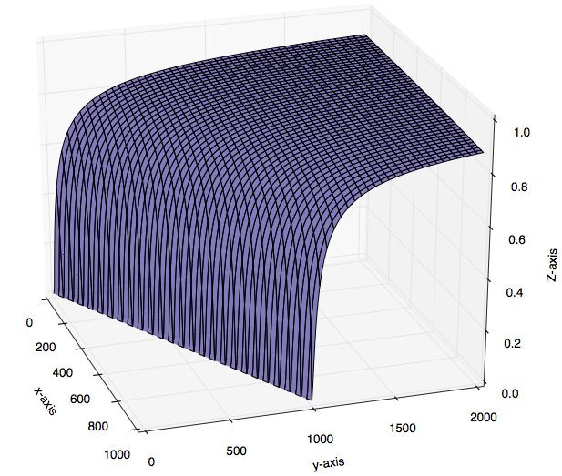
Figure 1.1. These figures, which will be described more accurately below, illustrate LemmaΒ 3.1 and TheoremΒ 3.1. The image on the left represents the graph of the restriction of a conditional cumulative distribution function
FΞ³:(x,y)βˆˆβ„2→ℙ​({Y≀y}|X=x)∈[0,1]:superscript𝐹𝛾π‘₯𝑦superscriptℝ2β†’β„™conditionalπ‘Œπ‘¦π‘‹π‘₯01F^{\gamma}:(x,y)\in\mathbb{R}^{2}\to\mathbb{P}(\{Y\leq y\}|X=x)\in[0,1]
which is associated to the joint law pX,Ysubscriptπ‘π‘‹π‘Œp_{X,Y} of an adapted coupling (X,Y,(Ξ©,π’œ,β„™))π‘‹π‘ŒΞ©π’œβ„™(X,Y,(\Omega,\mathcal{A},\mathbb{P})) according to DefinitionΒ 1.1 : as it will be shown by TheoremΒ 4.1, it turns out to coincide with some causal transport plan γ𝛾\gamma, when ℝℝ\mathbb{R} is endowed with a suitable probabilistic filtration; above, the "​X=x​""𝑋π‘₯""X=x" refers to a desintegration of measure. The image on the right represents the graph of a function T:ℝ→ℝ:𝑇→ℝℝT:\mathbb{R}\to\mathbb{R} such that (X,T​(X),(Ξ©,π’œ,β„™))π‘‹π‘‡π‘‹Ξ©π’œβ„™(X,T(X),(\Omega,\mathcal{A},\mathbb{P})) is an adapted coupling for any real-valued random variable X𝑋X : as it will be pointed out below, the joint law pX,T​(X)subscript𝑝𝑋𝑇𝑋p_{X,T(X)} actually boils down to a deterministic causal transport plan. Within models, in both cases illustrated above, the upper half-plane (resp. the lower half-plane) above (resp. below) the first diagonal corresponds to cases where a response signal was sent at a time y𝑦y relatively after (resp. before) the time xπ‘₯x where the entry signal has been received. Depending on those two regions of the plane, curves may exhibit quite distinct aspects.

In section 2, we fix the notation with a particular emphasize on the filtration which we take on ℝℝ\mathbb{R}, and on the transport kernel which is used to define the filtration generated by a transport plan adopted in [11] ; within models, recall that this filtration encapsulates the information flow which is required to perform the plan as time evolves. In section 3, DefinitionΒ 3.1 provides a recall of the latter, within this specific framework, which is used to state the definition of causal transport plans which we adopt here. Then, LemmaΒ 3.1 mentions a characterization for such plans between Borel probability measures on ℝℝ\mathbb{R}, which is then used to shorten subsequent proofs : it stands on specific properties of a conditional probability cumulative distribution function

FΞ³:(x,y)βˆˆβ„2β†’Fxγ​(y)βˆˆβ„,:superscript𝐹𝛾π‘₯𝑦superscriptℝ2β†’subscriptsuperscript𝐹𝛾π‘₯𝑦ℝF^{\gamma}:(x,y)\in\mathbb{R}^{2}\to F^{\gamma}_{x}(y)\in\mathbb{R},

which is Borel measurable (respectively increasing and cΓ d-lΓ g) along the first (resp. second) variable ; the french acronym cΓ d-lΓ g refers to right-continuous functions with left limits. To obtain a better understanding of those latter plans within the particular circumstances which we encounter in this context, we then state an accurate characterization to identify the deterministic ones, in TheoremΒ 3.1, while LemmaΒ 3.2 provides details to clearly grasp its origin. As a byproduct, this theorem yields a strong motivation for the representation provided by the adapted couplings adopted in DefinitionΒ 1.1. A proof that this representation actually holds in the general case is provided in TheoremΒ 4.1 of sectionΒ 4, where, under mild hypothesis, it is then applied to obtain, in CorollaryΒ 4.1, the existence of a solution to the problem which is stated above, from adapted tools of mass transport. It may be remarked that some arguments adopted from optimal transport can facilitate the identification of the optima. Furthermore, several examples are provided, notably from the jump times of a simple Poisson process, which are aimed to provide some explicit illustrations of specificities of the related causal transport plans, within this framework.

2. Preliminaries and notation

In this whole work, for the sake of clarity, we set 𝕋=ℝ𝕋ℝ\mathbb{T}=\mathbb{R}, while ℝℝ\mathbb{R} is endowed with its usual topology, whose associated Borel Οƒβˆ’limit-from𝜎\sigma- field is denoted by ℬ​(ℝ)ℬℝ\mathcal{B}(\mathbb{R}). The set of Borel probability measures on (ℝ,ℬ​(ℝ))ℝℬℝ(\mathbb{R},\mathcal{B}(\mathbb{R})) is denoted by M1​(ℝ)subscript𝑀1ℝM_{1}(\mathbb{R}). Whenever π’’βŠ‚β„¬β€‹(ℝ)𝒒ℬℝ\mathcal{G}\subset\mathcal{B}(\mathbb{R}) denotes a sigma-field, and ν∈M1​(ℝ)𝜈subscript𝑀1ℝ\nu\in M_{1}(\mathbb{R}), the set of Ξ½βˆ’limit-from𝜈\nu- negligible subsets is defined by 𝒩ν:={NβŠ‚β„:βˆƒAβˆˆβ„¬β€‹(ℝ),NβŠ‚A,and,​ν​(A)=0}assignsuperscriptπ’©πœˆconditional-set𝑁ℝformulae-sequence𝐴ℬℝformulae-sequence𝑁𝐴and,𝜈𝐴0\mathcal{N}^{\nu}:=\{N\subset\mathbb{R}:\ \exists A\in\mathcal{B}(\mathbb{R}),\ N\subset A,\ \text{and,}\ \nu(A)=0\}. Moreover 𝒒νsuperscriptπ’’πœˆ\mathcal{G}^{\nu}, which we still call here the Ξ½βˆ’limit-from𝜈\nu- completion of 𝒒𝒒\mathcal{G}, denotes the smallest Οƒβˆ’limit-from𝜎\sigma- fields on ℝℝ\mathbb{R} which contains both all the elements of 𝒒𝒒\mathcal{G} and all the elements of 𝒩νsuperscriptπ’©πœˆ\mathcal{N}^{\nu} ; notice that the negligible sets are taken with respect to the whole ℬ​(ℝ)ℬℝ\mathcal{B}(\mathbb{R}), while stating the Ξ½βˆ’limit-from𝜈\nu- completion of a sub Οƒβˆ’limit-from𝜎\sigma- field 𝒒𝒒\mathcal{G}. For much details on probabilities and on specific tools as we use it subsequently, we refer to [1]. For ν∈M1​(ℝ)𝜈subscript𝑀1ℝ\nu\in M_{1}(\mathbb{R}), the unique extension of ν𝜈\nu to ℬ​(ℝ)νℬsuperscriptβ„πœˆ\mathcal{B}(\mathbb{R})^{\nu} is still denoted by ν𝜈\nu, which doesn’t seem to yield any confusion below. We endow ℝℝ\mathbb{R} with the filtration (ℬt​(ℝ))tβˆˆπ•‹subscriptsubscriptℬ𝑑ℝ𝑑𝕋(\mathcal{B}_{t}(\mathbb{R}))_{t\in\mathbb{T}}, i.e. ℬs​(ℝ)βŠ‚β„¬t​(ℝ)βŠ‚β„¬β€‹(ℝ)subscriptℬ𝑠ℝsubscriptℬ𝑑ℝℬℝ\mathcal{B}_{s}(\mathbb{R})\subset\mathcal{B}_{t}(\mathbb{R})\subset\mathcal{B}(\mathbb{R}), βˆ€s,tβˆˆπ•‹for-all𝑠𝑑𝕋\forall s,t\in\mathbb{T} such that s≀t𝑠𝑑s\leq t, which is defined by

ℬt(ℝ)={Aβˆˆβ„¬(ℝ):AβŠ‚]βˆ’βˆž,t[or[t,+∞[βŠ‚A},\mathcal{B}_{t}(\mathbb{R})=\{A\in\mathcal{B}(\mathbb{R}):A\subset]-\infty,t[\ \text{or}\ [t,+\infty[\subset A\},

so that ℬt​(ℝ)subscriptℬ𝑑ℝ\mathcal{B}_{t}(\mathbb{R}) is equivalently defined by ℬt​(ℝ)=σ​(π’žt)subscriptβ„¬π‘‘β„πœŽsubscriptπ’žπ‘‘\mathcal{B}_{t}(\mathbb{R})=\sigma(\mathcal{C}_{t}), the smallest Οƒβˆ’limit-from𝜎\sigma- field on ℝℝ\mathbb{R} which contains all the subsets which constitute

π’žt={]βˆ’βˆž,a],a<t},\mathcal{C}_{t}=\{]-\infty,a],a<t\}, (2.2)

βˆ€tβˆˆπ•‹for-all𝑑𝕋\forall t\in\mathbb{T}. The cartesian product ℝ×ℝℝℝ\mathbb{R}\times\mathbb{R} is endowed with its usual product topology which turns it into a Polish space, while the associated Borel sigma field is denoted by ℬ​(ℝ×ℝ)ℬℝℝ\mathcal{B}(\mathbb{R}\times\mathbb{R}) ; M1​(ℝ×ℝ)subscript𝑀1ℝℝM_{1}(\mathbb{R}\times\mathbb{R}) denotes the set of Borel probability measures defined on the measurable space (ℝ×ℝ,ℬ​(ℝ×ℝ))ℝℝℬℝℝ(\mathbb{R}\times\mathbb{R},\mathcal{B}(\mathbb{R}\times\mathbb{R})), while we adapt conventional notation analogous to the case of ℝℝ\mathbb{R} for completions. Given Ξ·,ν∈M1​(ℝ)πœ‚πœˆsubscript𝑀1ℝ\eta,\nu\in M_{1}(\mathbb{R}), in optimal transport ([10], [13], [15], [18]), a probability γ∈M1​(ℝ×ℝ)𝛾subscript𝑀1ℝℝ\gamma\in M_{1}(\mathbb{R}\times\mathbb{R}) is said to be a transport plan from Ξ·πœ‚\eta to ν𝜈\nu, if and only if, its first marginal is Ξ·πœ‚\eta (i.e. p1⋆​γ=Ξ·subscriptsubscript𝑝1β‹†π›Ύπœ‚{p_{1}}_{\star}\gamma=\eta) and its second marginal is ν𝜈\nu (i.e. p2⋆​γ=Ξ½subscriptsubscript𝑝2β‹†π›Ύπœˆ{p_{2}}_{\star}\gamma=\nu), p1:(x,y)βˆˆβ„Γ—β„β†’xβˆˆβ„:subscript𝑝1π‘₯𝑦ℝℝ→π‘₯ℝp_{1}:(x,y)\in\mathbb{R}\times\mathbb{R}\to x\in\mathbb{R} (resp. p2:(x,y)βˆˆβ„Γ—β„β†’yβˆˆβ„:subscript𝑝2π‘₯𝑦ℝℝ→𝑦ℝp_{2}:(x,y)\in\mathbb{R}\times\mathbb{R}\to y\in\mathbb{R}) denoting the canonical projections functions, while p1⋆​γsubscriptsubscript𝑝1⋆𝛾{p_{1}}_{\star}\gamma (resp. p2⋆​γsubscriptsubscript𝑝2⋆𝛾{p_{2}}_{\star}\gamma) denotes the pushforward (see [1]) of γ𝛾\gamma by p1subscript𝑝1p_{1} (resp. by p2subscript𝑝2p_{2}) ; p1⋆​γ​(A)=γ​(A×ℝ)subscriptsubscript𝑝1⋆𝛾𝐴𝛾𝐴ℝ{p_{1}}_{\star}\gamma(A)=\gamma(A\times\mathbb{R}) (resp. p2⋆​γ​(B)=γ​(ℝ×B)subscriptsubscript𝑝2⋆𝛾𝐡𝛾ℝ𝐡{p_{2}}_{\star}\gamma(B)=\gamma(\mathbb{R}\times B)), βˆ€Aβˆˆβ„¬β€‹(ℝ)for-all𝐴ℬℝ\forall A\in\mathcal{B}(\mathbb{R}) (resp. βˆ€Bβˆˆβ„¬β€‹(ℝ)for-all𝐡ℬℝ\forall B\in\mathcal{B}(\mathbb{R})). Then,

Π​(Ξ·,Ξ½)={γ∈M1​(ℝ×ℝ):p1⋆​γ=Ξ·,p2⋆​γ=Ξ½}Ξ πœ‚πœˆconditional-set𝛾subscript𝑀1ℝℝformulae-sequencesubscriptsubscript𝑝1β‹†π›Ύπœ‚subscriptsubscript𝑝2β‹†π›Ύπœˆ\Pi(\eta,\nu)=\{\gamma\in M_{1}(\mathbb{R}\times\mathbb{R}):{p_{1}}_{\star}\gamma=\eta,{p_{2}}_{\star}\gamma=\nu\}

denotes the set of transport plans from Ξ·πœ‚\eta to ν𝜈\nu.

To describe accurately cases where the mass is splitted within the transport, recall that for any Ξ³βˆˆΞ β€‹(Ξ·,Ξ½)π›ΎΞ πœ‚πœˆ\gamma\in\Pi(\eta,\nu), there exists a function xβˆˆβ„β†’QΞ³x∈M1​(ℝ)π‘₯ℝ→superscriptsubscript𝑄𝛾π‘₯subscript𝑀1ℝx\in\mathbb{R}\to Q_{\gamma}^{x}\in M_{1}(\mathbb{R}) (see [6], [7]), such that the function

Ο•B:xβˆˆβ„β†’QΞ³x​(B)βˆˆβ„:subscriptitalic-ϕ𝐡π‘₯ℝ→subscriptsuperscript𝑄π‘₯𝛾𝐡ℝ\phi_{B}:x\in\mathbb{R}\to Q^{x}_{\gamma}(B)\in\mathbb{R} (2.3)

is Borel measurable, βˆ€Bβˆˆβ„¬β€‹(ℝ)for-all𝐡ℬℝ\forall B\in\mathcal{B}(\mathbb{R}), and

γ​(AΓ—B)=∫AQΞ³x​(B)​η​(d​x),βˆ€A,Bβˆˆβ„¬β€‹(ℝ),formulae-sequence𝛾𝐴𝐡subscript𝐴superscriptsubscript𝑄𝛾π‘₯π΅πœ‚π‘‘π‘₯for-all𝐴𝐡ℬℝ\gamma(A\times B)=\int_{A}Q_{\gamma}^{x}(B)\eta(dx),\ \forall A,B\in\mathcal{B}(\mathbb{R}), (2.4)

the latter denoting a Lebesgue integral with respect to the Borel probability measure Ξ·πœ‚\eta, which is well defined from the previous hypothesis onΒ (2.3) ; within mass transport models, QΞ³x​(B)subscriptsuperscript𝑄π‘₯𝛾𝐡Q^{x}_{\gamma}(B) may be interpreted as the proportion of the mass located at xβˆˆβ„π‘₯ℝx\in\mathbb{R} which is carried to Bβˆˆβ„¬β€‹(ℝ)𝐡ℬℝB\in\mathcal{B}(\mathbb{R}), since QΞ³subscript𝑄𝛾Q_{\gamma} coincides with a desintegration kernel of γ𝛾\gamma with respect to the canonical projection p1subscript𝑝1p_{1} (see [5]), outside an Ξ·βˆ’limit-fromπœ‚\eta- negligible set ; we have, for any Aβˆˆβ„¬β€‹(ℝ)𝐴ℬℝA\in\mathcal{B}(\mathbb{R}), QΞ³x​(A)=γ​({p2∈A}|p1=x)superscriptsubscript𝑄𝛾π‘₯𝐴𝛾conditionalsubscript𝑝2𝐴subscript𝑝1π‘₯Q_{\gamma}^{x}(A)=\gamma(\{p_{2}\in A\}|p_{1}=x), Ξ·βˆ’a.s.formulae-sequenceπœ‚π‘Žπ‘ \eta-a.s., where "​p1=x​""subscript𝑝1π‘₯""p_{1}=x" refers here to a desintegration of measure. Subsequently, any such function QΞ³subscript𝑄𝛾Q_{\gamma} will be called a transport kernel associated to γ𝛾\gamma ; it is unique up to an Ξ·βˆ’limit-fromπœ‚\eta- negligible set, which will justify to take Ξ·βˆ’limit-fromπœ‚\eta- completions below. Futher, for xβˆˆβ„π‘₯ℝx\in\mathbb{R}, FxΞ³subscriptsuperscript𝐹𝛾π‘₯F^{\gamma}_{x} denotes the cumulative distribution function of QΞ³xsuperscriptsubscript𝑄𝛾π‘₯Q_{\gamma}^{x} ; FxΞ³(a)=QΞ³x(]βˆ’βˆž,a])F^{\gamma}_{x}(a)=Q_{\gamma}^{x}(]-\infty,a]), βˆ€aβˆˆβ„for-allπ‘Žβ„\forall a\in\mathbb{R}, and we set

FΞ³:(x,y)βˆˆβ„2β†’Fxγ​(y)βˆˆβ„,:superscript𝐹𝛾π‘₯𝑦superscriptℝ2β†’subscriptsuperscript𝐹𝛾π‘₯𝑦ℝF^{\gamma}:(x,y)\in\mathbb{R}^{2}\to F^{\gamma}_{x}(y)\in\mathbb{R},

to which we refer to as a conditional cumulative distribution function associated to γ𝛾\gamma, as it may depend on the choice of QΞ³subscript𝑄𝛾Q_{\gamma}. Furthermore, given a real-valued random variable X𝑋X which is defined on a probability space (Ξ©,π’œ,β„™)Ξ©π’œβ„™(\Omega,\mathcal{A},\mathbb{P}), that is, a function X:Ω→ℝ:𝑋→ΩℝX:\Omega\to\mathbb{R} whose level sets {Ο‰βˆˆΞ©:X​(Ο‰)≀l}βˆˆπ’œconditional-setπœ”Ξ©π‘‹πœ”π‘™π’œ\{\omega\in\Omega:X(\omega)\leq l\}\in\mathcal{A} are all contained in π’œπ’œ\mathcal{A}, βˆ€lβˆˆβ„for-all𝑙ℝ\forall l\in\mathbb{R}, for short and once given AβŠ‚β„π΄β„A\subset\mathbb{R}, we may use the notation {X∈A}𝑋𝐴\{X\in A\} to denote the inverse image Xβˆ’1​(A):={Ο‰βˆˆΞ©:X​(Ο‰)∈A}assignsuperscript𝑋1𝐴conditional-setπœ”Ξ©π‘‹πœ”π΄X^{-1}(A):=\{\omega\in\Omega:X(\omega)\in A\}, while we use the notation Eℙ​[X]subscript𝐸ℙdelimited-[]𝑋E_{\mathbb{P}}[X] to denote the mathematical expectation of X𝑋X under the probability β„™β„™\mathbb{P} ; Eℙ​[X]:=∫ΩX​(Ο‰)​ℙ​(d​ω)assignsubscript𝐸ℙdelimited-[]𝑋subscriptΞ©π‘‹πœ”β„™π‘‘πœ”E_{\mathbb{P}}[X]:=\int_{\Omega}X(\omega)\mathbb{P}(d\omega) denotes a Lebesgue integral with respect to the probability measure β„™β„™\mathbb{P} whenever X𝑋X is β„™βˆ’limit-fromβ„™\mathbb{P}- integrable (i.e. Eℙ​[|X|]<+∞subscript𝐸ℙdelimited-[]𝑋E_{\mathbb{P}}[|X|]<+\infty), in which case Eℙ​[X]βˆˆβ„subscript𝐸ℙdelimited-[]𝑋ℝE_{\mathbb{P}}[X]\in\mathbb{R}, while we set Eℙ​[X]=+∞subscript𝐸ℙdelimited-[]𝑋E_{\mathbb{P}}[X]=+\infty whenever Xβ‰₯0𝑋0X\geq 0, β„™βˆ’a.s.formulae-sequenceβ„™π‘Žπ‘ \mathbb{P}-a.s. and X𝑋X is not β„™βˆ’limit-fromβ„™\mathbb{P}- integrable. The law of the random variable X𝑋X is denoted by pX∈M1​(ℝ)subscript𝑝𝑋subscript𝑀1ℝp_{X}\in M_{1}(\mathbb{R}), where pX​(A)=ℙ​(Xβˆ’1​(A))=ℙ​({X∈A})subscript𝑝𝑋𝐴ℙsuperscript𝑋1𝐴ℙ𝑋𝐴p_{X}(A)=\mathbb{P}(X^{-1}(A))=\mathbb{P}(\{X\in A\}), βˆ€Aβˆˆβ„¬β€‹(ℝ)for-all𝐴ℬℝ\forall A\in\mathcal{B}(\mathbb{R}), while further assuming that Y:Ω→ℝ:π‘Œβ†’Ξ©β„Y:\Omega\to\mathbb{R} denotes a random variable defined on the same probability space as X𝑋X, pX,Y∈M1​(ℝ×ℝ)subscriptπ‘π‘‹π‘Œsubscript𝑀1ℝℝp_{X,Y}\in M_{1}(\mathbb{R}\times\mathbb{R}) denotes the joint law of X𝑋X and Yπ‘ŒY, that is, the pushforward pX,Y:=(X,Y)⋆​ℙassignsubscriptπ‘π‘‹π‘Œsubscriptπ‘‹π‘Œβ‹†β„™p_{X,Y}:=(X,Y)_{\star}\mathbb{P} of the probability measure β„™β„™\mathbb{P} by the measurable function (X,Y):Ο‰βˆˆΞ©β†’(X​(Ο‰),Y​(Ο‰))βˆˆβ„Γ—β„:π‘‹π‘Œπœ”Ξ©β†’π‘‹πœ”π‘Œπœ”β„β„(X,Y):\omega\in\Omega\to(X(\omega),Y(\omega))\in\mathbb{R}\times\mathbb{R}, so that pX,Y​(A)=ℙ​({(X,Y)∈A})subscriptπ‘π‘‹π‘Œπ΄β„™π‘‹π‘Œπ΄p_{X,Y}(A)=\mathbb{P}(\{(X,Y)\in A\}), βˆ€Aβˆˆβ„¬β€‹(ℝ×ℝ)for-all𝐴ℬℝℝ\forall A\in\mathcal{B}(\mathbb{R}\times\mathbb{R}); whenever X𝑋X is β„™βˆ’limit-fromβ„™\mathbb{P}- independent to Yπ‘ŒY we denote by pXβŠ—pYtensor-productsubscript𝑝𝑋subscriptπ‘π‘Œp_{X}\otimes p_{Y} their joint law pX,Ysubscriptπ‘π‘‹π‘Œp_{X,Y}. Finally, given a probability space (Ξ©,π’œ,β„™)Ξ©π’œβ„™(\Omega,\mathcal{A},\mathbb{P}), if Cβˆˆπ’œπΆπ’œC\in\mathcal{A} is such that ℙ​(C)>0ℙ𝐢0\mathbb{P}(C)>0, we apply the standard notation ℙ​(A|C)=ℙ​(A∩C)ℙ​(C)β„™conditional𝐴𝐢ℙ𝐴𝐢ℙ𝐢\mathbb{P}(A|C)=\frac{\mathbb{P}(A\cap C)}{\mathbb{P}(C)}, βˆ€Aβˆˆπ’œfor-allπ΄π’œ\forall A\in\mathcal{A}, as it is used in DefinitionΒ 1.1 with C={Xβ‰₯t}𝐢𝑋𝑑C=\{X\geq t\}, tβˆˆπ•‹π‘‘π•‹t\in\mathbb{T}, while for any Aβˆˆπ’œπ΄π’œA\in\mathcal{A}, πŸ™A:Ω→ℝ:subscript1𝐴→Ωℝ\mathds{1}_{A}:\Omega\to\mathbb{R} denotes here the indicator function of A𝐴A ; πŸ™A​(Ο‰)=1subscript1π΄πœ”1\mathds{1}_{A}(\omega)=1 if Ο‰βˆˆAπœ”π΄\omega\in A, while πŸ™A​(Ο‰)=0subscript1π΄πœ”0\mathds{1}_{A}(\omega)=0 if Ο‰βˆ‰Aπœ”π΄\omega\notin A, βˆ€Ο‰βˆˆΞ©for-allπœ”Ξ©\forall\omega\in\Omega.

3. Causal mass transport between Borel probabilities on the set of real numbers.

3.1. The filtration generated by a transport plan, a characterization

We recall some conventional terminology adopted in [11], which will be required subsequently.

Definition 3.1.

Let Ξ·,ν∈M1​(ℝ)πœ‚πœˆsubscript𝑀1ℝ\eta,\nu\in M_{1}(\mathbb{R}), and Ξ³βˆˆΞ β€‹(Ξ·,Ξ½)π›ΎΞ πœ‚πœˆ\gamma\in\Pi(\eta,\nu). The filtration (𝒒t​(Ξ³))tβˆˆπ•‹subscriptsubscript𝒒𝑑𝛾𝑑𝕋(\mathcal{G}_{t}(\gamma))_{t\in\mathbb{T}} generated by γ𝛾\gamma is defined, for any tβˆˆπ•‹π‘‘π•‹t\in\mathbb{T}, by

𝒒t(Ξ³)=Οƒ(Ο•B:Bβˆˆβ„¬t(ℝ),Ξ½(βˆ‚B)=0)Ξ·;\mathcal{G}_{t}(\gamma)=\sigma(\phi_{B}:B\in\mathcal{B}_{t}(\mathbb{R}),\ \nu(\partial B)=0)^{\eta};

the Ξ·βˆ’limit-fromπœ‚\eta- completion of the smallest sigma field which turns into measurable functions all the functions Ο•Bsubscriptitalic-ϕ𝐡\phi_{B} as inΒ (2.3) such that Bβˆˆβ„¬t​(ℝ)𝐡subscriptℬ𝑑ℝB\in\mathcal{B}_{t}(\mathbb{R}) and ν​(βˆ‚B)=0𝜈𝐡0\nu(\partial B)=0. The set Ξ c​(Ξ·,Ξ½)subscriptΞ π‘πœ‚πœˆ\Pi_{c}(\eta,\nu) of causal (or adapted) transport plans γ𝛾\gamma from Ξ·πœ‚\eta to ν𝜈\nu is defined by

Ξ c​(Ξ·,Ξ½)={Ξ³βˆˆΞ β€‹(Ξ·,Ξ½):𝒒t​(Ξ³)βŠ‚β„¬t​(ℝ)Ξ·,βˆ€tβˆˆπ•‹}.subscriptΞ π‘πœ‚πœˆconditional-setπ›ΎΞ πœ‚πœˆformulae-sequencesubscript𝒒𝑑𝛾subscriptℬ𝑑superscriptβ„πœ‚for-all𝑑𝕋\Pi_{c}(\eta,\nu)=\{\gamma\in\Pi(\eta,\nu):\mathcal{G}_{t}(\gamma)\subset\mathcal{B}_{t}(\mathbb{R})^{\eta},\ \forall t\in\mathbb{T}\}.
Lemma 3.1.

Let Ξ·,ν∈M1​(ℝ)πœ‚πœˆsubscript𝑀1ℝ\eta,\nu\in M_{1}(\mathbb{R}), Ξ³βˆˆΞ β€‹(Ξ·,Ξ½)π›ΎΞ πœ‚πœˆ\gamma\in\Pi(\eta,\nu), and further denote by QΞ³:xβˆˆβ„β†’QΞ³x∈M1​(ℝ):subscript𝑄𝛾π‘₯ℝ→superscriptsubscript𝑄𝛾π‘₯subscript𝑀1ℝQ_{\gamma}:x\in\mathbb{R}\to Q_{\gamma}^{x}\in M_{1}(\mathbb{R}) a transport kernel associated to γ𝛾\gamma byΒ (2.4). Then the following assertions are equivalent :

  1. (i)

    γ∈Πc​(Ξ·,Ξ½)𝛾subscriptΞ π‘πœ‚πœˆ\gamma\in\Pi_{c}(\eta,\nu)

  2. (ii)

    For any tβˆˆπ•‹π‘‘π•‹t\in\mathbb{T} such that Ξ·([t,+∞[)>0\eta([t,+\infty[)>0, βˆ€Aβˆˆβ„¬t​(ℝ)for-all𝐴subscriptℬ𝑑ℝ\forall A\in\mathcal{B}_{t}(\mathbb{R}),and for all xβ‰₯tπ‘₯𝑑x\geq t outside an Ξ·βˆ’limit-fromπœ‚\eta- negligible set, we have

    Qγx(A)=γ({p2∈A}|{p1∈[t,+∞[});Q_{\gamma}^{x}(A)=\gamma(\{p_{2}\in A\}|\{p_{1}\in[t,+\infty[\});

    conditional probability, with respect to an event.

  3. (iii)

    For any tβˆˆπ•‹π‘‘π•‹t\in\mathbb{T} such that Ξ·([t,+∞[)>0\eta([t,+\infty[)>0, and for any a<tπ‘Žπ‘‘a<t, βˆƒca,tβˆˆβ„subscriptπ‘π‘Žπ‘‘β„\exists c_{a,t}\in\mathbb{R} such that we have

    Fxγ​(a)=ca,t,βˆ€xβ‰₯t,outside anβ€‹Ξ·βˆ’negligible set,formulae-sequencesuperscriptsubscript𝐹π‘₯π›Ύπ‘Žsubscriptπ‘π‘Žπ‘‘for-allπ‘₯𝑑outside anπœ‚negligible setF_{x}^{\gamma}(a)=c_{a,t},\ \forall x\geq t,\ \text{outside an}\ \eta-\text{negligible set},

    FxΞ³:ℝ→[0,1]:superscriptsubscript𝐹π‘₯𝛾→ℝ01F_{x}^{\gamma}:\mathbb{R}\to[0,1] denoting the cumulative distribution function of QΞ³xsuperscriptsubscript𝑄𝛾π‘₯Q_{\gamma}^{x}, βˆ€xβˆˆβ„for-allπ‘₯ℝ\forall x\in\mathbb{R}.

Proof:Β Since the definitions yield

ℬt​(ℝ)=ρtβˆ’1​(ℬ​(ℝ))={{xβˆˆβ„:ρt​(x)∈A}:Aβˆˆβ„¬β€‹(ℝ)},subscriptℬ𝑑ℝsuperscriptsubscriptπœŒπ‘‘1ℬℝconditional-setconditional-setπ‘₯ℝsubscriptπœŒπ‘‘π‘₯𝐴𝐴ℬℝ\mathcal{B}_{t}(\mathbb{R})=\rho_{t}^{-1}(\mathcal{B}(\mathbb{R}))=\{\{x\in\mathbb{R}:\rho_{t}(x)\in A\}:A\in\mathcal{B}(\mathbb{R})\},

where the function ρt:sβˆˆβ„β†’min⁑(s,t)βˆˆβ„:subscriptπœŒπ‘‘π‘ β„β†’π‘ π‘‘β„\rho_{t}:s\in\mathbb{R}\to\min(s,t)\in\mathbb{R} is continuous, βˆ€tβˆˆπ•‹for-all𝑑𝕋\forall t\in\mathbb{T}, and ρt∘ρu=ρmin⁑(t,u),subscriptπœŒπ‘‘subscriptπœŒπ‘’subscriptπœŒπ‘‘π‘’\rho_{t}\circ\rho_{u}=\rho_{\min(t,u)}, βˆ€t,uβˆˆπ•‹for-all𝑑𝑒𝕋\forall t,u\in\mathbb{T}, ∘\circ denoting the usual pullback of functions, from [11] we first deduce that, for any tβˆˆπ•‹π‘‘π•‹t\in\mathbb{T}, we have

𝒒t(Ξ³)=Οƒ(Ο•A:Aβˆˆβ„¬t(ℝ))Ξ·;\mathcal{G}_{t}(\gamma)=\sigma(\phi_{A}:A\in\mathcal{B}_{t}(\mathbb{R}))^{\eta}; (3.5)

since ℬt​(ℝ)subscriptℬ𝑑ℝ\mathcal{B}_{t}(\mathbb{R}) is also the Οƒβˆ’limit-from𝜎\sigma- field generated by {ρtβˆ’1​(F):F​closed subset of​ℝ}conditional-setsuperscriptsubscriptπœŒπ‘‘1𝐹𝐹closed subset ofℝ\{\rho_{t}^{-1}(F):\ F\ \text{closed subset of}\ \mathbb{R}\}, the latter equationΒ (3.5) can also be checked readily by a monotone class argument, once noticed that, since ρtsubscriptπœŒπ‘‘\rho_{t} is continuous, for any closed set FβŠ‚β„πΉβ„F\subset\mathbb{R}, the holding condition λ​({y>0:ν​(βˆ‚(ρtβˆ’1​(dFβˆ’1​([0,y]))))>0})=0πœ†conditional-set𝑦0𝜈superscriptsubscriptπœŒπ‘‘1superscriptsubscript𝑑𝐹10𝑦00\lambda(\{y>0:\nu(\partial(\rho_{t}^{-1}(d_{F}^{-1}([0,y]))))>0\})=0, where Ξ»πœ†\lambda denotes the Lebesgue mesure, and where dF:xβˆˆβ„β†’infy∈F|xβˆ’y|βˆˆβ„:subscript𝑑𝐹π‘₯ℝ→subscriptinfimum𝑦𝐹π‘₯𝑦ℝd_{F}:x\in\mathbb{R}\to\inf_{y\in F}|x-y|\in\mathbb{R}, yields the existence of a decreasing sequence (Bn)nβˆˆβ„•subscriptsubscript𝐡𝑛𝑛ℕ(B_{n})_{n\in\mathbb{N}} of closed subsets of the form ρtβˆ’1(dFβˆ’1(]βˆ’βˆž,tn]))\rho_{t}^{-1}(d_{F}^{-1}(]-\infty,t_{n}])), for some tn>0subscript𝑑𝑛0t_{n}>0, which further satisfy ν​(βˆ‚Bn)=0𝜈subscript𝐡𝑛0\nu(\partial B_{n})=0, Bnβˆˆβ„¬t​(ℝ)subscript𝐡𝑛subscriptℬ𝑑ℝB_{n}\in\mathcal{B}_{t}(\mathbb{R}), βˆ€nβˆˆβ„•for-all𝑛ℕ\forall n\in\mathbb{N} while ρtβˆ’1​(F)=β‹‚nβˆˆβ„•BnsuperscriptsubscriptπœŒπ‘‘1𝐹subscript𝑛ℕsubscript𝐡𝑛\rho_{t}^{-1}(F)=\bigcap_{n\in\mathbb{N}}B_{n}, so that ϕρtβˆ’1​(F)=limnβ†’βˆžΟ•Bnsubscriptitalic-Ο•superscriptsubscriptπœŒπ‘‘1𝐹subscript→𝑛subscriptitalic-Ο•subscript𝐡𝑛\phi_{\rho_{t}^{-1}(F)}=\lim_{n\to\infty}\phi_{B_{n}}, Ξ·βˆ’a.s.formulae-sequenceπœ‚π‘Žπ‘ \eta-a.s., and therefore ϕρtβˆ’1​(F)subscriptitalic-Ο•superscriptsubscriptπœŒπ‘‘1𝐹\phi_{\rho_{t}^{-1}(F)} is 𝒒t​(Ξ³)βˆ’limit-fromsubscript𝒒𝑑𝛾\mathcal{G}_{t}(\gamma)- measurable. FromΒ (3.5), we first notice that γ∈Πc​(Ξ·,Ξ½)𝛾subscriptΞ π‘πœ‚πœˆ\gamma\in\Pi_{c}(\eta,\nu), if an only if,

Qγ​(A)=Eη​[Qγ​(A)|ℬt​(ℝ)Ξ·],Ξ·βˆ’a.s.formulae-sequencesubscript𝑄𝛾𝐴subscriptπΈπœ‚delimited-[]conditionalsubscript𝑄𝛾𝐴subscriptℬ𝑑superscriptβ„πœ‚πœ‚π‘Žπ‘ Q_{\gamma}(A)=E_{\eta}[Q_{\gamma}(A)|\mathcal{B}_{t}(\mathbb{R})^{\eta}],\ \eta-a.s. (3.6)

for all Aβˆˆβ„¬t​(ℝ)𝐴subscriptℬ𝑑ℝA\in\mathcal{B}_{t}(\mathbb{R}), βˆ€tβˆˆπ•‹for-all𝑑𝕋\forall t\in\mathbb{T} ; the right-hand term ofΒ (3.6) denotes a conditional expectation with respect to the ΟƒπœŽ\sigma- field ℬt​(ℝ)Ξ·subscriptℬ𝑑superscriptβ„πœ‚\mathcal{B}_{t}(\mathbb{R})^{\eta}, where tβˆˆπ•‹π‘‘π•‹t\in\mathbb{T}. We now turn to the main part of the proof. First assume (i)𝑖(i), and let tβˆˆβ„π‘‘β„t\in\mathbb{R}. For Aβˆˆβ„¬t​(ℝ)𝐴subscriptℬ𝑑ℝA\in\mathcal{B}_{t}(\mathbb{R}), from the very definition of the conditional expectation with respect to a sigma field (for instance see [5], [7]), and from the properties of the filtration (ℬt​(ℝ))tβˆˆπ•‹subscriptsubscriptℬ𝑑ℝ𝑑𝕋(\mathcal{B}_{t}(\mathbb{R}))_{t\in\mathbb{T}} just recalled above, it directly follows that

EΞ·[QΞ³(A)|ℬt(ℝ)Ξ·]=QΞ³(A)πŸ™]βˆ’βˆž,t[+Ξ³({p2∈A}|{p1∈[t,+∞[})πŸ™[t,+∞[,Ξ·βˆ’a.s.,E_{\eta}[Q_{\gamma}(A)|\mathcal{B}_{t}(\mathbb{R})^{\eta}]=Q_{\gamma}(A)\mathds{1}_{]-\infty,t[}+\gamma(\{p_{2}\in A\}|\{p_{1}\in[t,+\infty[\})\mathds{1}_{[t,+\infty[},\ \eta-a.s.,

if Ξ·([t,+∞[)>0\eta([t,+\infty[)>0, whileΒ (3.6) already holds as soon as Ξ·([t,+∞[)=0\eta([t,+\infty[)=0. As a consequence,Β (3.6) holds for all Aβˆˆβ„¬t​(ℝ)𝐴subscriptℬ𝑑ℝA\in\mathcal{B}_{t}(\mathbb{R}), and βˆ€tβˆˆπ•‹for-all𝑑𝕋\forall t\in\mathbb{T}, if and only if,

Ξ³({p2∈A}|{p1∈[t,+∞[})πŸ™[t,+∞[=QΞ³(A)πŸ™[t,+∞[,Ξ·βˆ’a.s.,\gamma(\{p_{2}\in A\}|\{p_{1}\in[t,+\infty[\})\mathds{1}_{[t,+\infty[}=Q_{\gamma}(A)\mathds{1}_{[t,+\infty[},\ \eta-a.s.,

holds, for all Aβˆˆβ„¬t​(ℝ)𝐴subscriptℬ𝑑ℝA\in\mathcal{B}_{t}(\mathbb{R}), and βˆ€tβˆˆπ•‹for-all𝑑𝕋\forall t\in\mathbb{T} such that Ξ·([t,+∞[)>0\eta([t,+\infty[)>0, which is (i​i)𝑖𝑖(ii) : we have proved that (i)𝑖(i) is equivalent to (i​i)𝑖𝑖(ii). On the other hand, since for tβˆˆπ•‹π‘‘π•‹t\in\mathbb{T} and a<tπ‘Žπ‘‘a<t, ]βˆ’βˆž,a]βˆˆβ„¬t(ℝ)]-\infty,a]\in\mathcal{B}_{t}(\mathbb{R}), (i​i)𝑖𝑖(ii) yields (i​i​i)𝑖𝑖𝑖(iii) as a particular case, by taking

ca,t=Ξ³({p2∈]βˆ’βˆž,a]}|{p1∈[t,+∞[})∈[0,1].c_{a,t}=\gamma(\{p_{2}\in]-\infty,a]\}|\{p_{1}\in[t,+\infty[\})\in[0,1]. (3.7)

Finally, assuming that (i​i​i)𝑖𝑖𝑖(iii) holds, for tβˆˆπ•‹π‘‘π•‹t\in\mathbb{T} such that Ξ·([t,+∞[)>0\eta([t,+\infty[)>0, and a<tπ‘Žπ‘‘a<t, we notice that we still obtainΒ (3.7), so that we have (i​i)𝑖𝑖(ii) for all Aβˆˆβ„¬t​(ℝ)𝐴subscriptℬ𝑑ℝA\in\mathcal{B}_{t}(\mathbb{R}) of the form ]βˆ’βˆž,a]]-\infty,a], a<tπ‘Žπ‘‘a<t. Since ℬt​(ℝ)=σ​(π’žt)subscriptβ„¬π‘‘β„πœŽsubscriptπ’žπ‘‘\mathcal{B}_{t}(\mathbb{R})=\sigma(\mathcal{C}_{t}), where π’žtβŠ‚β„¬β€‹(ℝ)subscriptπ’žπ‘‘β„¬β„\mathcal{C}_{t}\subset\mathcal{B}(\mathbb{R}) is given byΒ (2.2), (i​i)𝑖𝑖(ii) follows from a monotone class argument (see [5]). Β Β  Β Β 

Refer to caption
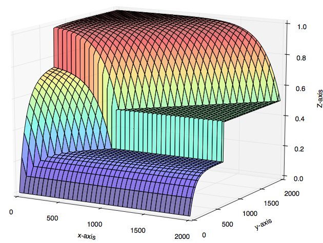
Figure 3.2. This figure illustrates LemmaΒ 3.1. Representation of the restriction to the square [0,2000]Γ—[0,2000]0200002000[0,2000]\times[0,2000] of a conditional cumulative distribution function FΞ³superscript𝐹𝛾F^{\gamma}, which is associated to the causal transport plan
Ξ³=12​pX,X+Z+14​pXβŠ—Ξ΄t0+14​pXβŠ—pX,𝛾12subscript𝑝𝑋𝑋𝑍tensor-product14subscript𝑝𝑋subscript𝛿subscript𝑑0tensor-product14subscript𝑝𝑋subscript𝑝𝑋\gamma=\frac{1}{2}p_{X,X+Z}+\frac{1}{4}p_{X}\otimes\delta_{t_{0}}+\frac{1}{4}p_{X}\otimes p_{X},
where t0=700subscript𝑑0700t_{0}=700, and where X𝑋X, and Z𝑍Z denote two β„™βˆ’limit-fromβ„™\mathbb{P}- independent real valued random variables defined on a same probability space (Ξ©,π’œ,β„™)Ξ©π’œβ„™(\Omega,\mathcal{A},\mathbb{P}), whose laws are given by pX=ℰ​(1100)subscript𝑝𝑋ℰ1100p_{X}=\mathcal{E}\left(\frac{1}{100}\right), and by pZ=ℰ​(1200)subscript𝑝𝑍ℰ1200p_{Z}=\mathcal{E}\left(\frac{1}{200}\right) ; ℰ​(Ξ²)∈M1​(ℝ)ℰ𝛽subscript𝑀1ℝ\mathcal{E}(\beta)\in M_{1}(\mathbb{R}) denotes the so-called exponential law of parameter Ξ²βˆˆβ„+⋆𝛽superscriptsubscriptℝ⋆\beta\in\mathbb{R}_{+}^{\star}, that is, the Borel probability measure absolutely continuous with respect to the Lebesgue measure, whose density fΞ²:ℝ→ℝ:subscript𝑓𝛽→ℝℝf_{\beta}:\mathbb{R}\to\mathbb{R} is given by
fβ​(x)=β​exp⁑(βˆ’Ξ²β€‹x)β€‹πŸ™[0,+∞[​(x),βˆ€xβˆˆβ„.f_{\beta}(x)=\beta\exp(-\beta x)\mathds{1}_{[0,+\infty[}(x),\ \forall x\in\mathbb{R}.

3.2. Deterministic causal transport plans

Let η∈M1​(ℝ)πœ‚subscript𝑀1ℝ\eta\in M_{1}(\mathbb{R}), let T:ℝ→ℝ:𝑇→ℝℝT:\mathbb{R}\to\mathbb{R} be a Borel measurable function, and define Ξ³T=(Iℝ,T)⋆​ηsubscript𝛾𝑇subscriptsubscriptπΌβ„π‘‡β‹†πœ‚\gamma_{T}=(I_{\mathbb{R}},T)_{\star}\eta, the deterministic transport plan of Ξ·πœ‚\eta by T𝑇T ; we can set QΞ³Tx=Ξ΄T​(x)subscriptsuperscript𝑄π‘₯subscript𝛾𝑇subscript𝛿𝑇π‘₯Q^{x}_{\gamma_{T}}=\delta_{T(x)}, βˆ€xβˆˆβ„for-allπ‘₯ℝ\forall x\in\mathbb{R}, Ξ΄ysubscript𝛿𝑦\delta_{y} denoting the Dirac mass (see [1]) centered on yβˆˆβ„π‘¦β„y\in\mathbb{R}, βˆ€yβˆˆβ„for-all𝑦ℝ\forall y\in\mathbb{R}, while Ξ³Tsubscript𝛾𝑇\gamma_{T} coincides with the pushforward measure of Ξ·πœ‚\eta by the measurable function

(Iℝ,T):xβˆˆβ„β†’(x,T​(x))βˆˆβ„Γ—β„,:subscript𝐼ℝ𝑇π‘₯ℝ→π‘₯𝑇π‘₯ℝℝ(I_{\mathbb{R}},T):x\in\mathbb{R}\to(x,T(x))\in\mathbb{R}\times\mathbb{R},

so that (Iℝ,T)⋆​η​(C)=η​({xβˆˆβ„:(x,T​(x))∈C})subscriptsubscriptπΌβ„π‘‡β‹†πœ‚πΆπœ‚conditional-setπ‘₯ℝπ‘₯𝑇π‘₯𝐢(I_{\mathbb{R}},T)_{\star}{\eta}(C)=\eta(\{x\in\mathbb{R}:(x,T(x))\in C\}), βˆ€Cβˆˆβ„¬β€‹(ℝ×ℝ)for-all𝐢ℬℝℝ\forall C\in\mathcal{B}(\mathbb{R}\times\mathbb{R}). Further recall that, within those specific hypothesis, fromΒ (3.5) we obtain

𝒒t​(Ξ³T)=𝒒tT,subscript𝒒𝑑subscript𝛾𝑇superscriptsubscript𝒒𝑑𝑇\mathcal{G}_{t}(\gamma_{T})=\mathcal{G}_{t}^{T}, (3.8)

where

𝒒tT={Tβˆ’1​(A):Aβˆˆβ„¬t​(ℝ)}Ξ·,superscriptsubscript𝒒𝑑𝑇superscriptconditional-setsuperscript𝑇1𝐴𝐴subscriptβ„¬π‘‘β„πœ‚\mathcal{G}_{t}^{T}=\{T^{-1}(A)\ :\ A\in\mathcal{B}_{t}(\mathbb{R})\}^{\eta},

βˆ€tβˆˆπ•‹for-all𝑑𝕋\forall t\in\mathbb{T} ; Tβˆ’1​(A)={xβˆˆβ„:T​(x)∈A}superscript𝑇1𝐴conditional-setπ‘₯ℝ𝑇π‘₯𝐴T^{-1}(A)=\{x\in\mathbb{R}:T(x)\in A\} still denotes the inverse image of Aβˆˆβ„¬β€‹(ℝ)𝐴ℬℝA\in\mathcal{B}(\mathbb{R}) by the function T𝑇T. Finally, for the sake of consistency with [11] and for short, given η∈M1​(ℝ)πœ‚subscript𝑀1ℝ\eta\in M_{1}(\mathbb{R}), subsequently T𝑇T will be said to be adapted (or causal), if and only if, Ξ³T∈Πc​(Ξ·,Ξ½)subscript𝛾𝑇subscriptΞ π‘πœ‚πœˆ\gamma_{T}\in\Pi_{c}(\eta,\nu), where Ξ½=Tβ‹†β€‹Ξ·πœˆsubscriptπ‘‡β‹†πœ‚\nu=T_{\star}\eta, if and only if,

𝒒tTβŠ‚β„¬t​(ℝ)Ξ·,βˆ€tβˆˆπ•‹,formulae-sequencesuperscriptsubscript𝒒𝑑𝑇subscriptℬ𝑑superscriptβ„πœ‚for-all𝑑𝕋\mathcal{G}_{t}^{T}\subset\mathcal{B}_{t}(\mathbb{R})^{\eta},\ \forall t\in\mathbb{T},

where the last equivalence follows fromΒ (3.8); again, Tβ‹†β€‹Ξ·βˆˆM1​(ℝ)subscriptπ‘‡β‹†πœ‚subscript𝑀1ℝT_{\star}\eta\in M_{1}(\mathbb{R}) denotes the pushforward or direct image of η∈M1​(ℝ)πœ‚subscript𝑀1ℝ\eta\in M_{1}(\mathbb{R}) by the Borel measurable function T:ℝ→ℝ:𝑇→ℝℝT:\mathbb{R}\to\mathbb{R}, that is T⋆​η​(A)=η​({xβˆˆβ„:T​(x)∈A})subscriptπ‘‡β‹†πœ‚π΄πœ‚conditional-setπ‘₯ℝ𝑇π‘₯𝐴T_{\star}\eta(A)=\eta(\{x\in\mathbb{R}:T(x)\in A\}), βˆ€Aβˆˆβ„¬β€‹(ℝ)for-all𝐴ℬℝ\forall A\in\mathcal{B}(\mathbb{R}).

Lemma 3.2.

Let η∈M1​(ℝ)πœ‚subscript𝑀1ℝ\eta\in M_{1}(\mathbb{R}), and let T:ℝ→ℝ:𝑇→ℝℝT:\mathbb{R}\to\mathbb{R} be a Borel measurable function such that T𝑇T is adapted, i.e. Tβˆ’1​(ℬt​(ℝ))βŠ‚β„¬t​(ℝ)Ξ·superscript𝑇1subscriptℬ𝑑ℝsubscriptℬ𝑑superscriptβ„πœ‚T^{-1}(\mathcal{B}_{t}(\mathbb{R}))\subset\mathcal{B}_{t}(\mathbb{R})^{\eta}, βˆ€tβˆˆπ•‹for-all𝑑𝕋\forall t\in\mathbb{T}. Further assume that we have

η​({xβˆˆβ„:T​(x)<x})>0.πœ‚conditional-setπ‘₯ℝ𝑇π‘₯π‘₯0\eta(\{x\in\mathbb{R}:T(x)<x\})>0. (3.9)

Then, the following assertions are satisfied :

  1. (i)

    βˆ€tβˆˆπ•‹for-all𝑑𝕋\forall t\in\mathbb{T}, βˆ€Aβˆˆβ„¬β€‹(ℝ)for-all𝐴ℬℝ\forall A\in\mathcal{B}(\mathbb{R}) such that either AβŠ‚]βˆ’βˆž,t[A\subset]-\infty,t[ or [t,+∞[βŠ‚A[t,+\infty[\subset A, the following implication holds :

    Ξ·({xβ‰₯t:T(x)∈A})>0⟹η({xβˆˆβ„:T(x)∈A}|[t,+∞[)=1.\eta(\{x\geq t:T(x)\in A\})>0\implies\eta(\{x\in\mathbb{R}:T(x)\in A\}|[t,+\infty[)=1.
  2. (ii)

    Let

    D={tβˆˆβ„:η​({xβ‰₯t:T​(x)<t})>0}.𝐷conditional-setπ‘‘β„πœ‚conditional-setπ‘₯𝑑𝑇π‘₯𝑑0D=\{t\in\mathbb{R}:\eta(\{x\geq t:T(x)<t\})>0\}.

    Then, Dβ‰ βˆ…π·D\neq\emptyset, and there exists a unique t0βˆˆβ„subscript𝑑0ℝt_{0}\in\mathbb{R} which is such that t0<tsubscript𝑑0𝑑t_{0}<t, βˆ€t∈Dfor-all𝑑𝐷\forall t\in D, and

    Ξ·({xβˆˆβ„:T(x)=t0}|[t,+∞[)=1,βˆ€t∈D.\eta(\{x\in\mathbb{R}:T(x)=t_{0}\}|[t,+\infty[)=1,\ \forall t\in D.
  3. (iii)

    infDβˆˆβ„infimum𝐷ℝ\inf D\in\mathbb{R} is not attained and we have

    η(]infD,+∞[)>0\eta(]\inf D,+\infty[)>0

    and

    Ξ·({xβˆˆβ„:T(x)=t0}|]infD,+∞[)=1.\eta(\{x\in\mathbb{R}:T(x)=t_{0}\}|]\inf D,+\infty[)=1.
  4. (iv)

    The following hold :

    {Ξ·({x≀t0:T(x)β‰₯x})=Ξ·(]βˆ’βˆž,t0])Ξ·(]t0,+∞[)>0Ξ·({xβˆˆβ„:T(x)=t0}|]t0,+∞[)=1.\begin{cases}\eta(\{x\leq t_{0}:T(x)\geq x\})=\eta(]-\infty,t_{0}])\\ \eta(]t_{0},+\infty[)>0\\ \eta(\{x\in\mathbb{R}:T(x)=t_{0}\}|]t_{0},+\infty[)=1\end{cases}.

Proof:Β Since Ξ³T=(Iℝ,T)β‹†β€‹Ξ·βˆˆΞ c​(Ξ·,Ξ½)subscript𝛾𝑇subscriptsubscriptπΌβ„π‘‡β‹†πœ‚subscriptΞ π‘πœ‚πœˆ\gamma_{T}=(I_{\mathbb{R}},T)_{\star}\eta\in\Pi_{c}(\eta,\nu), where Ξ½=Tβ‹†β€‹Ξ·πœˆsubscriptπ‘‡β‹†πœ‚\nu=T_{\star}\eta, LemmaΒ 3.1 applies. Hence, assume that tβˆˆπ•‹π‘‘π•‹t\in\mathbb{T} and Aβˆˆβ„¬t​(ℝ)𝐴subscriptℬ𝑑ℝA\in\mathcal{B}_{t}(\mathbb{R}) are such that η​({xβ‰₯t:T​(x)∈A})>0πœ‚conditional-setπ‘₯𝑑𝑇π‘₯𝐴0\eta(\{x\geq t:T(x)\in A\})>0 ; in particular, Ξ·([t,+∞[)>0\eta([t,+\infty[)>0. As we can state

QΞ³Tx​(A)=Ξ΄T​(x)​(A)=πŸ™A​(T​(x))=πŸ™Tβˆ’1​(A)​(x),βˆ€xβˆˆβ„,formulae-sequencesubscriptsuperscript𝑄π‘₯subscript𝛾𝑇𝐴subscript𝛿𝑇π‘₯𝐴subscript1𝐴𝑇π‘₯subscript1superscript𝑇1𝐴π‘₯for-allπ‘₯ℝQ^{x}_{\gamma_{T}}(A)=\delta_{T(x)}(A)=\mathds{1}_{A}(T(x))=\mathds{1}_{T^{-1}(A)}(x),\ \forall x\in\mathbb{R},

QΞ³Tsubscript𝑄subscript𝛾𝑇Q_{\gamma_{T}} denoting a transport kernel for Ξ³Tsubscript𝛾𝑇\gamma_{T} recalled above, from LemmaΒ 3.1 we obtain

πŸ™Tβˆ’1​(A)πŸ™[t,+∞[=Ξ³T({p2∈A}|{p1∈[t,+∞[})πŸ™[t,+∞[,Ξ·βˆ’a.s.,\mathds{1}_{T^{-1}(A)}\mathds{1}_{[t,+\infty[}=\gamma_{T}(\{p_{2}\in A\}|\{p_{1}\in[t,+\infty[\})\mathds{1}_{[t,+\infty[},\ \eta-a.s.,

so that η​({xβ‰₯t:T​(x)∈A})>0πœ‚conditional-setπ‘₯𝑑𝑇π‘₯𝐴0\eta(\{x\geq t:T(x)\in A\})>0 implies Ξ³T({p2∈A}|{p1∈[t,+∞[})=1\gamma_{T}(\{p_{2}\in A\}|\{p_{1}\in[t,+\infty[\})=1, from which the implication (i)𝑖(i) follows. Further noticing that

η​({xβˆˆβ„:T​(x)<x})=η​(⋃qβˆˆβ„š{xβ‰₯q:T​(x)<q}),πœ‚conditional-setπ‘₯ℝ𝑇π‘₯π‘₯πœ‚subscriptπ‘žβ„šconditional-setπ‘₯π‘žπ‘‡π‘₯π‘ž\eta(\{x\in\mathbb{R}:T(x)<x\})=\eta\left(\bigcup_{q\in\mathbb{Q}}\{x\geq q:T(x)<q\}\right),

and that a countable union of negligible sets is again negligible, we obtain Dβ‰ βˆ…π·D\neq\emptyset fromΒ (3.9). Then, we choose any t∈D𝑑𝐷t\in D, and define

t0=inf({yβˆˆβ„:η​({xβ‰₯t:T​(x)<y})β‰₯η​({xβ‰₯t:T​(x)<t})}).subscript𝑑0infimumconditional-setπ‘¦β„πœ‚conditional-setπ‘₯𝑑𝑇π‘₯π‘¦πœ‚conditional-setπ‘₯𝑑𝑇π‘₯𝑑t_{0}=\inf(\{y\in\mathbb{R}:\eta(\{x\geq t:T(x)<y\})\geq\eta(\{x\geq t:T(x)<t\})\}).

Together with (i)𝑖(i), from the definitions, it is then an easy exercise to check that t0βˆˆβ„subscript𝑑0ℝt_{0}\in\mathbb{R} doesn’t depend on the choice of t∈D𝑑𝐷t\in D, while it meets the required hypothesis. Finally, the rest of the statement results by following the successive steps, while applying (i)𝑖(i) as far as necessary. Β Β  Β Β 

Theorem 3.1.

Let η∈M1​(ℝ)πœ‚subscript𝑀1ℝ\eta\in M_{1}(\mathbb{R}), let T:ℝ→ℝ:𝑇→ℝℝT:\mathbb{R}\to\mathbb{R} be a Borel measurable function, set Ξ½=Tβ‹†β€‹ΞΌπœˆsubscriptπ‘‡β‹†πœ‡\nu=T_{\star}\mu, and still define Ξ³T=(Iℝ,T)⋆​ηsubscript𝛾𝑇subscriptsubscriptπΌβ„π‘‡β‹†πœ‚\gamma_{T}=(I_{\mathbb{R}},T)_{\star}\eta to be the deterministic transport plan of Ξ·πœ‚\eta by T𝑇T. Then, Ξ³T∈Πc​(Ξ·,Ξ½)subscript𝛾𝑇subscriptΞ π‘πœ‚πœˆ\gamma_{T}\in\Pi_{c}(\eta,\nu), if and only if, T𝑇T satisfies one among the two hypothesis below :

  1. (1)

    T​(x)β‰₯x𝑇π‘₯π‘₯T(x)\geq x, Ξ·βˆ’a.s.formulae-sequenceπœ‚π‘Žπ‘ \eta-a.s.

  2. (2)

    βˆƒt0βˆˆβ„subscript𝑑0ℝ\exists t_{0}\in\mathbb{R} which is such that, βˆ€x≀t0for-allπ‘₯subscript𝑑0\forall x\leq t_{0} outside an Ξ·βˆ’limit-fromπœ‚\eta- negligible set, we have T​(x)β‰₯x𝑇π‘₯π‘₯T(x)\geq x, and for any x>t0π‘₯subscript𝑑0x>t_{0} outside an Ξ·βˆ’limit-fromπœ‚\eta- negligible set, we have T​(x)=t0𝑇π‘₯subscript𝑑0T(x)=t_{0}.

Proof:Β Assuming that one among (1)1(1) or (2)2(2) is satisfied, it is enough to notice that ℬt​(ℝ)=σ​(π’žt)subscriptβ„¬π‘‘β„πœŽsubscriptπ’žπ‘‘\mathcal{B}_{t}(\mathbb{R})=\sigma(\mathcal{C}_{t}), where π’žtsubscriptπ’žπ‘‘\mathcal{C}_{t} is given byΒ (2.2), so that we easily check that Ξ³T∈Πc​(Ξ·,Ξ½)subscript𝛾𝑇subscriptΞ π‘πœ‚πœˆ\gamma_{T}\in\Pi_{c}(\eta,\nu), as 𝒒tTβŠ‚β„¬t​(ℝ)Ξ·superscriptsubscript𝒒𝑑𝑇subscriptℬ𝑑superscriptβ„πœ‚\mathcal{G}_{t}^{T}\subset\mathcal{B}_{t}(\mathbb{R})^{\eta}, βˆ€tβˆˆπ•‹for-all𝑑𝕋\forall t\in\mathbb{T} ; recall thatΒ (3.8) holds. Conversely, assuming that Ξ³T∈Πc​(Ξ·,Ξ½)subscript𝛾𝑇subscriptΞ π‘πœ‚πœˆ\gamma_{T}\in\Pi_{c}(\eta,\nu), the result follows from LemmaΒ 3.2. Β Β  Β Β 

Remark:Β  (2)2(2) above is clearly equivalent to : βˆƒt0βˆˆβ„subscript𝑑0ℝ\exists t_{0}\in\mathbb{R} and a non-negative Borel measurable function gT:ℝ→[0,+∞[g_{T}:\mathbb{R}\to[0,+\infty[, such that

T​(x)=(x+gT​(x))β€‹πŸ™]βˆ’βˆž,t0]​(x)+t0β€‹πŸ™]t0,+∞[​(x),Ξ·βˆ’a.e..T(x)=(x+g_{T}(x))\mathds{1}_{]-\infty,t_{0}]}(x)+t_{0}\mathds{1}_{]t_{0},+\infty[}(x),\ \eta-a.e..
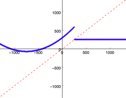
Refer to caption
Refer to caption
Refer to caption
Refer to caption
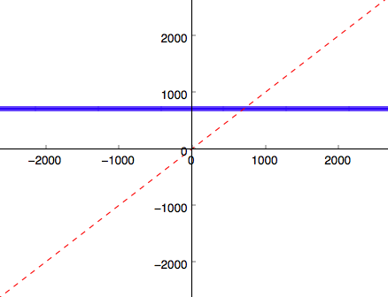
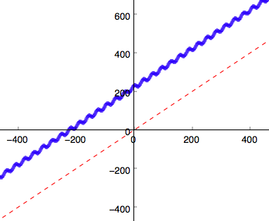
Figure 3.3. This figures illustrate TheoremΒ 3.1. In red, the first diagonal of the plane. In blue, the representation of the restriction of the graph of the Borel measurable function T:ℝ→ℝ:𝑇→ℝℝT:\mathbb{R}\to\mathbb{R}, given by, from the image on the left to the image on the right,
T​(x)=c,βˆ€xβˆˆβ„,formulae-sequence𝑇π‘₯𝑐for-allπ‘₯ℝT(x)=c,\ \forall x\in\mathbb{R},
with c=700𝑐700c=700, by
T​(x)=(x+z0)β€‹πŸ™]βˆ’βˆž,t0]​(x)+t0β€‹πŸ™]t0,+∞[​(x),βˆ€xβˆˆβ„,T(x)=(x+z_{0})\mathds{1}_{]-\infty,t_{0}]}(x)+t_{0}\mathds{1}_{]t_{0},+\infty[}(x),\ \forall x\in\mathbb{R},
with t0=30subscript𝑑030t_{0}=30 and z0=200subscript𝑧0200z_{0}=200, by
T:xβˆˆβ„β†’(a​x2+b​x+c)β€‹πŸ™]βˆ’βˆž,t0]+t0β€‹πŸ™]t0,+∞[​(x)βˆˆβ„,T:x\in\mathbb{R}\to(ax^{2}+bx+c)\mathds{1}_{]-\infty,t_{0}]}+t_{0}\mathds{1}_{]t_{0},+\infty[}(x)\in\mathbb{R},
with t0=250subscript𝑑0250t_{0}=250, a=11500π‘Ž11500a=\frac{1}{1500}, b=1𝑏1b=1, and c=300𝑐300c=300, and finally by
T:xβˆˆβ„β†’x+a​cos⁑(b​x)+cβˆˆβ„,:𝑇π‘₯ℝ→π‘₯π‘Žπ‘π‘₯𝑐ℝT:x\in\mathbb{R}\to x+a\cos(bx)+c\in\mathbb{R},
where a=10π‘Ž10a=10, b=15𝑏15b=\frac{1}{5}, and c=220𝑐220c=220. For any η∈M1​(ℝ)πœ‚subscript𝑀1ℝ\eta\in M_{1}(\mathbb{R}), those functions T𝑇T induce a deterministic causal transport plan Ξ³T=(Iℝ,T)β‹†β€‹Ξ·βˆˆΞ c​(Ξ·,Ξ½)subscript𝛾𝑇subscriptsubscriptπΌβ„π‘‡β‹†πœ‚subscriptΞ π‘πœ‚πœˆ\gamma_{T}=(I_{\mathbb{R}},T)_{\star}\eta\in\Pi_{c}(\eta,\nu) of Ξ·πœ‚\eta to Ξ½=Tβ‹†β€‹Ξ·πœˆsubscriptπ‘‡β‹†πœ‚\nu=T_{\star}\eta.

As a first practical consequence of TheoremΒ 3.1, we get :

Corollary 3.1.

Let T:ℝ→ℝ:𝑇→ℝℝT:\mathbb{R}\to\mathbb{R} be a Borel measurable function, η∈M1​(ℝ)πœ‚subscript𝑀1ℝ\eta\in M_{1}(\mathbb{R}), and assume that Ξ½=Tβ‹†β€‹Ξ·πœˆsubscriptπ‘‡β‹†πœ‚\nu=T_{\star}\eta and Ξ·πœ‚\eta are diffuse (i.e. η​({x})=ν​({x})=0πœ‚π‘₯𝜈π‘₯0\eta(\{x\})=\nu(\{x\})=0, βˆ€xβˆˆβ„for-allπ‘₯ℝ\forall x\in\mathbb{R}), and that Ξ·(]t,+∞[)>0\eta(]t,+\infty[)>0, βˆ€tβˆˆπ•‹for-all𝑑𝕋\forall t\in\mathbb{T} ; for instance, Ξ·πœ‚\eta has a cumulative distribution function which is strictly increasing on ]y,+∞[]y,+\infty[ for some yβˆˆβ„π‘¦β„y\in\mathbb{R}. Then, T𝑇T is adapted, if and only if,

T​(x)β‰₯x,Ξ·βˆ’a.s..formulae-sequence𝑇π‘₯π‘₯πœ‚π‘Žπ‘ T(x)\geq x,\ \eta-a.s..

Β Β  Β Β 

Example 3.1.

Let a,bβˆˆβ„π‘Žπ‘β„a,b\in\mathbb{R}, and define T:xβˆˆβ„β†’a​x+bβˆˆβ„:𝑇π‘₯β„β†’π‘Žπ‘₯𝑏ℝT:x\in\mathbb{R}\to ax+b\in\mathbb{R} ; recall again that within those hypothesis, given η∈M1​(ℝ)πœ‚subscript𝑀1ℝ\eta\in M_{1}(\mathbb{R}), T𝑇T is said to be adapted, if and only if, Ξ³=(Iℝ,T)β‹†β€‹Ξ·βˆˆΞ c​(Ξ·,Ξ½)𝛾subscriptsubscriptπΌβ„π‘‡β‹†πœ‚subscriptΞ π‘πœ‚πœˆ\gamma=(I_{\mathbb{R}},T)_{\star}\eta\in\Pi_{c}(\eta,\nu), where Ξ½=Tβ‹†β€‹Ξ·πœˆsubscriptπ‘‡β‹†πœ‚\nu=T_{\star}\eta, if and only if, Tβˆ’1​(ℬt​(ℝ))βŠ‚β„¬t​(ℝ)Ξ·superscript𝑇1subscriptℬ𝑑ℝsubscriptℬ𝑑superscriptβ„πœ‚T^{-1}(\mathcal{B}_{t}(\mathbb{R}))\subset\mathcal{B}_{t}(\mathbb{R})^{\eta}, βˆ€tβˆˆπ•‹for-all𝑑𝕋\forall t\in\mathbb{T}.

  • β€’

    Assuming that Ξ·=𝒩​(0,1)πœ‚π’©01\eta=\mathcal{N}(0,1) (the Gauss law), T𝑇T is adapted, if and only if, either a=0π‘Ž0a=0, or both a=1π‘Ž1a=1 and bβ‰₯0𝑏0b\geq 0.

  • β€’

    If Ξ·=ℰ​(1)πœ‚β„°1\eta=\mathcal{E}(1) (exponential law) then T𝑇T is adapted, if and only if, either a=0π‘Ž0a=0, or both aβ‰₯1π‘Ž1a\geq 1 and bβ‰₯0𝑏0b\geq 0.

4. Characterization of adapted couplings and probabilistic optimization.

The following TheoremΒ 4.1 will allow to address the problem stated in the introduction by using tools of causal optimal transport, in CorollaryΒ 4.1.

Theorem 4.1.
  1. (1)

    Let Ξ·,ν∈M1​(ℝ)πœ‚πœˆsubscript𝑀1ℝ\eta,\nu\in M_{1}(\mathbb{R}). Then, for any γ∈Πc​(Ξ·,Ξ½)𝛾subscriptΞ π‘πœ‚πœˆ\gamma\in\Pi_{c}(\eta,\nu), there exists an adapted coupling (X,Y,(Ξ©,π’œ,β„™))∈C​p​la​(Ξ·,Ξ½)π‘‹π‘ŒΞ©π’œβ„™πΆπ‘subscriptπ‘™π‘Žπœ‚πœˆ(X,Y,(\Omega,\mathcal{A},\mathbb{P}))\in Cpl_{a}(\eta,\nu) such that pX,Y=Ξ³subscriptπ‘π‘‹π‘Œπ›Ύp_{X,Y}=\gamma, where pX,Y∈M1​(ℝ×ℝ)subscriptπ‘π‘‹π‘Œsubscript𝑀1ℝℝp_{X,Y}\in M_{1}(\mathbb{R}\times\mathbb{R}) denotes the joint law of the random variables X:Ω→ℝ:𝑋→ΩℝX:\Omega\to\mathbb{R} and Y:Ω→ℝ:π‘Œβ†’Ξ©β„Y:\Omega\to\mathbb{R} on the probability space (Ξ©,π’œ,β„™)Ξ©π’œβ„™(\Omega,\mathcal{A},\mathbb{P}), and where C​p​la​(Ξ·,Ξ½)𝐢𝑝subscriptπ‘™π‘Žπœ‚πœˆCpl_{a}(\eta,\nu) (resp. Ξ c​(Ξ·,Ξ½)subscriptΞ π‘πœ‚πœˆ\Pi_{c}(\eta,\nu)) is given by DefinitionΒ 1.1 (resp. by DefinitionΒ 3.1).

  2. (2)

    For any adapted coupling (X,Y,(Ξ©,π’œ,β„™))∈C​p​la​(pX,pY)π‘‹π‘ŒΞ©π’œβ„™πΆπ‘subscriptπ‘™π‘Žsubscript𝑝𝑋subscriptπ‘π‘Œ(X,Y,(\Omega,\mathcal{A},\mathbb{P}))\in Cpl_{a}(p_{X},p_{Y}), we have

    pX,Y∈Πc​(pX,pY),subscriptπ‘π‘‹π‘ŒsubscriptΠ𝑐subscript𝑝𝑋subscriptπ‘π‘Œp_{X,Y}\in\Pi_{c}(p_{X},p_{Y}),

    pXsubscript𝑝𝑋p_{X} (resp. pYsubscriptπ‘π‘Œp_{Y}) denoting the probability law of X𝑋X (resp. of Yπ‘ŒY) on (Ξ©,π’œ,β„™)Ξ©π’œβ„™(\Omega,\mathcal{A},\mathbb{P}).

Proof:Β First assume that γ∈Πc​(Ξ·,Ξ½)𝛾subscriptΞ π‘πœ‚πœˆ\gamma\in\Pi_{c}(\eta,\nu), and define

{(Ξ©,π’œ,β„™)=(ℝ×ℝ,ℬ​(ℝ×ℝ)Ξ³,Ξ³)X=p1Y=p2Ο„=min⁑(p1,p2)Z=(Yβˆ’X)β€‹πŸ™{X≀τ};casesΞ©π’œβ„™β„β„β„¬superscriptℝℝ𝛾𝛾otherwise𝑋subscript𝑝1otherwiseπ‘Œsubscript𝑝2otherwise𝜏subscript𝑝1subscript𝑝2otherwiseπ‘π‘Œπ‘‹subscript1π‘‹πœotherwise\begin{cases}(\Omega,\mathcal{A},\mathbb{P})=(\mathbb{R}\times\mathbb{R},\mathcal{B}(\mathbb{R}\times\mathbb{R})^{\gamma},\gamma)\\ X=p_{1}\\ Y=p_{2}\\ \tau=\min(p_{1},p_{2})\\ Z=(Y-X)\mathds{1}_{\{X\leq\tau\}}\end{cases};

p1subscript𝑝1p_{1} (resp. p2subscript𝑝2p_{2}) still denotes the canonical projection on the first (resp. second) component of the product space ℝ×ℝℝℝ\mathbb{R}\times\mathbb{R}. Then, it is enough to check that (X,Y,(Ξ©,π’œ,β„™))π‘‹π‘ŒΞ©π’œβ„™(X,Y,(\Omega,\mathcal{A},\mathbb{P})) satisfies the axioms of DefinitionΒ 1.1 to obtain (1)1(1), which follows from LemmaΒ 3.1. Then, (2)2(2) follows by applying again LemmaΒ 3.1, (i​i​i)𝑖𝑖𝑖(iii), together with the definitions. Β Β  Β Β 

Refer to caption
Figure 4.4. This figure illustrates ExampleΒ 4.1, for 0<a<b0π‘Žπ‘0<a<b. From classical results (see 2/ in 1.7. of [8]), for Ξ³=pTa,Tb𝛾subscript𝑝subscriptπ‘‡π‘Žsubscript𝑇𝑏\gamma=p_{T_{a},T_{b}} it follows that we can choose
Fxγ​(y)=πŸ™]0,+∞[​(yβˆ’x)​(1βˆ’erf​(bβˆ’a2​(yβˆ’x))),F^{\gamma}_{x}(y)=\mathds{1}_{]0,+\infty[}(y-x)\left(1-\text{erf}\left(\frac{b-a}{\sqrt{2(y-x)}}\right)\right),
βˆ€(x,y)βˆˆβ„+×ℝfor-allπ‘₯𝑦subscriptℝℝ\forall(x,y)\in\mathbb{R}_{+}\times\mathbb{R}, where erf denotes the so-called error function, which is given by erf​(z)=2Ο€β€‹βˆ«0zexp⁑(βˆ’t2)​𝑑terf𝑧2πœ‹superscriptsubscript0𝑧superscript𝑑2differential-d𝑑\text{erf}(z)=\frac{2}{\sqrt{\pi}}\int_{0}^{z}\exp\left(-t^{2}\right)dt, βˆ€zβˆˆβ„+for-all𝑧subscriptℝ\forall z\in\mathbb{R}_{+}; ℝ+subscriptℝ\mathbb{R}_{+} is the support of pTasubscript𝑝subscriptπ‘‡π‘Žp_{T_{a}}. The figure represents the restriction of the graph of FΞ³superscript𝐹𝛾F^{\gamma}, for a=6π‘Ž6a=6 and b=11𝑏11b=11.
Example 4.1.

Let (Bt)t∈[0,+∞[(B_{t})_{t\in[0,+\infty[} be a standard real valued Brownian motion, starting from 00, which is defined on a β„™βˆ’limit-fromβ„™\mathbb{P}- complete probability space (Ξ©,π’œ,β„™)Ξ©π’œβ„™(\Omega,\mathcal{A},\mathbb{P}) (see [16]); this is the continuous LΓ©vy process associated to the Gauss law 𝒩​(0,1)𝒩01\mathcal{N}(0,1) which is an infinitely divisible distribution, while the law of this continuous stochastic process is the so-called Wiener measure, see [12], [16], [17], [19]. In particular, (Bt)t∈[0,+∞[(B_{t})_{t\in[0,+\infty[} is a family of gaussian random variables labeled by ℝ+subscriptℝ\mathbb{R}_{+}, such that on the one hand the function t∈[0,+∞[β†’Bt(Ο‰)βˆˆβ„t\in[0,+\infty[\to B_{t}(\omega)\in\mathbb{R} is continuous for any Ο‰βˆˆΞ©πœ”Ξ©\omega\in\Omega outside a β„™βˆ’limit-fromβ„™\mathbb{P}- negligible set, while on the other hand, for any s,t∈]0,+∞[s,t\in]0,+\infty[ such that s<t𝑠𝑑s<t, there exists two independent random variables G𝐺G and G~~𝐺\widetilde{G}, depending respectively on s𝑠s and on both s𝑠s and t𝑑t, defined on a same probability space, and with a same Gauss law pG=pG~=𝒩​(0,1)∈M1​(ℝ)subscript𝑝𝐺subscript𝑝~𝐺𝒩01subscript𝑀1ℝp_{G}=p_{\widetilde{G}}=\mathcal{N}(0,1)\in M_{1}(\mathbb{R}), such that the joint law pBs,Btsubscript𝑝subscript𝐡𝑠subscript𝐡𝑑p_{B_{s},B_{t}} of the two random variables Bs:Ω→ℝ:subscript𝐡𝑠→ΩℝB_{s}:\Omega\to\mathbb{R} and Bt:Ω→ℝ:subscript𝐡𝑑→ΩℝB_{t}:\Omega\to\mathbb{R} on (Ξ©,π’œ,β„™)Ξ©π’œβ„™(\Omega,\mathcal{A},\mathbb{P}) coincide with the joint law of the random variables s​G𝑠𝐺\sqrt{s}G and s​G+tβˆ’s​G~𝑠𝐺𝑑𝑠~𝐺\sqrt{s}G+\sqrt{t-s}\widetilde{G}, that is

pBs,Bt=ps​G,s​G+tβˆ’s​G~.subscript𝑝subscript𝐡𝑠subscript𝐡𝑑subscript𝑝𝑠𝐺𝑠𝐺𝑑𝑠~𝐺p_{B_{s},B_{t}}=p_{\sqrt{s}G,\sqrt{s}G+\sqrt{t-s}\widetilde{G}}.

For cβˆˆβ„π‘β„c\in\mathbb{R}, define the, β„™βˆ’limit-fromβ„™\mathbb{P}- almost surely finite, first passage time random variable

Tc:=inf({tβ‰₯0:Bt=c}),assignsubscript𝑇𝑐infimumconditional-set𝑑0subscript𝐡𝑑𝑐T_{c}:=\inf(\{t\geq 0:B_{t}=c\}),

which is a so-called stopping time with respect to the filtration generated by (Bt)t∈[0,+∞[(B_{t})_{t\in[0,+\infty[} (see [8]). Assuming that 0<a<b0π‘Žπ‘0<a<b, from TheoremΒ 4.1, we obtain

pTa,Tb∈Πc​(pTa,pTb),subscript𝑝subscriptπ‘‡π‘Žsubscript𝑇𝑏subscriptΠ𝑐subscript𝑝subscriptπ‘‡π‘Žsubscript𝑝subscript𝑇𝑏p_{T_{a},T_{b}}\in\Pi_{c}(p_{T_{a}},p_{T_{b}}),

pTasubscript𝑝subscriptπ‘‡π‘Žp_{T_{a}} (resp. pTbsubscript𝑝subscript𝑇𝑏p_{T_{b}}) denoting the probability law of Tasubscriptπ‘‡π‘ŽT_{a} (resp. of Tbsubscript𝑇𝑏T_{b}), while pTa,Tb=(Ta,Tb)β‹†β€‹β„™βˆˆM1​(ℝ×ℝ)subscript𝑝subscriptπ‘‡π‘Žsubscript𝑇𝑏subscriptsubscriptπ‘‡π‘Žsubscript𝑇𝑏⋆ℙsubscript𝑀1ℝℝp_{T_{a},T_{b}}=(T_{a},T_{b})_{\star}\mathbb{P}\in M_{1}(\mathbb{R}\times\mathbb{R}) denotes their joint law, on the probability space (Ξ©,π’œ,β„™)Ξ©π’œβ„™(\Omega,\mathcal{A},\mathbb{P}).

Corollary 4.1.

Assume that c:ℝ×ℝ→ℝ:𝑐→ℝℝℝc:\mathbb{R}\times\mathbb{R}\to\mathbb{R} is a non-negative and lower semi-continuous function, and let Ξ·,ν∈M1​(ℝ)πœ‚πœˆsubscript𝑀1ℝ\eta,\nu\in M_{1}(\mathbb{R}). Then, there exists an adapted coupling (X⋆,Y⋆,(Ω⋆,(X_{\star},Y_{\star},(\Omega_{\star}, π’œβ‹†,subscriptπ’œβ‹†\mathcal{A}_{\star}, ℙ⋆))∈Cpla(Ξ·,Ξ½)\mathbb{P}_{\star}))\in Cpl_{a}(\eta,\nu) which attains

inf({Eℙ​[c​(X,Y)]:(X,Y,(Ξ©,π’œ,β„™))∈C​p​la​(Ξ·,Ξ½)}),infimumconditional-setsubscript𝐸ℙdelimited-[]π‘π‘‹π‘Œπ‘‹π‘ŒΞ©π’œβ„™πΆπ‘subscriptπ‘™π‘Žπœ‚πœˆ\inf(\{E_{\mathbb{P}}[c(X,Y)]:(X,Y,(\Omega,\mathcal{A},\mathbb{P}))\in Cpl_{a}(\eta,\nu)\}), (4.10)

where C​p​la​(Ξ·,Ξ½)𝐢𝑝subscriptπ‘™π‘Žπœ‚πœˆCpl_{a}(\eta,\nu) denotes the set defined in DefinitionΒ 1.1. Moreover, this problem is equivalent to the causal (or adapted) Monge-Kantorovich problem

infγ∈Πc​(Ξ·,Ξ½)βˆ«β„Γ—β„c​(x,y)​γ​(d​x,d​y),subscriptinfimum𝛾subscriptΞ π‘πœ‚πœˆsubscriptℝℝ𝑐π‘₯𝑦𝛾𝑑π‘₯𝑑𝑦\inf_{\gamma\in\Pi_{c}(\eta,\nu)}\int_{\mathbb{R}\times\mathbb{R}}c(x,y)\gamma(dx,dy), (4.11)

where Ξ c​(Ξ·,Ξ½)subscriptΞ π‘πœ‚πœˆ\Pi_{c}(\eta,\nu) is given by DefinitionΒ 3.1. That is, γ∈Πc​(Ξ·,Ξ½)𝛾subscriptΞ π‘πœ‚πœˆ\gamma\in\Pi_{c}(\eta,\nu) attains the infimum ofΒ (4.11), if and only if, there exists some adapted coupling (X,Y,(Ξ©,π’œ,β„™))∈C​p​la​(Ξ·,Ξ½)π‘‹π‘ŒΞ©π’œβ„™πΆπ‘subscriptπ‘™π‘Žπœ‚πœˆ(X,Y,(\Omega,\mathcal{A},\mathbb{P}))\in Cpl_{a}(\eta,\nu) which attains the infimum ofΒ (4.10), and Ξ³=pX,Y𝛾subscriptπ‘π‘‹π‘Œ\gamma=p_{X,Y}, where pX,Ysubscriptπ‘π‘‹π‘Œp_{X,Y} denotes the joint law of the pair of random variables X:Ω→ℝ:𝑋→ΩℝX:\Omega\to\mathbb{R} and Y:Ω→ℝ:π‘Œβ†’Ξ©β„Y:\Omega\to\mathbb{R}, on the β„™βˆ’limit-fromβ„™\mathbb{P}- complete probability space (Ξ©,π’œ,β„™)Ξ©π’œβ„™(\Omega,\mathcal{A},\mathbb{P}).

Proof:Β From TheoremΒ 4.1, this optimization problem is equivalent to the causal Monge-Kantorovich problemΒ (4.11). Hence, the result follows from [11]. Β Β  Β Β 

Example 4.2.

For mβˆˆβ„•π‘šβ„•m\in\mathbb{N}, Ξ»>0πœ†0\lambda>0, denote by Γ​(m,1Ξ»)∈M1​(ℝ)Ξ“π‘š1πœ†subscript𝑀1ℝ\Gamma\left(m,\frac{1}{\lambda}\right)\in M_{1}(\mathbb{R}) the Borel probability measure absolutely continuous with respect to the Lebesgue measure, whose density ρm,1Ξ»:ℝ→ℝ:subscriptπœŒπ‘š1πœ†β†’β„β„\rho_{m,\frac{1}{\lambda}}:\mathbb{R}\to\mathbb{R} is given by

ρm,1λ​(x)=λ​exp⁑(βˆ’Ξ»β€‹x)​(λ​x)mβˆ’1(mβˆ’1)!β€‹πŸ™[0,+∞[​(x),βˆ€xβˆˆβ„;\rho_{m,\frac{1}{\lambda}}(x)=\lambda\exp(-\lambda x)\frac{(\lambda x)^{m-1}}{(m-1)!}\mathds{1}_{[0,+\infty[}(x),\ \forall x\in\mathbb{R};

those are particular cases of the so-called gamma distributions. For nβˆˆβ„•π‘›β„•n\in\mathbb{N}, and pβˆˆβ„•π‘β„•p\in\mathbb{N}, define

Ξ·=Γ​(n,1Ξ»)πœ‚Ξ“π‘›1πœ†\eta=\Gamma\left(n,\frac{1}{\lambda}\right)

and

Ξ½=Γ​(n+p,1Ξ»),πœˆΞ“π‘›π‘1πœ†\nu=\Gamma\left(n+p,\frac{1}{\lambda}\right),

for some λ∈]0,+∞[\lambda\in]0,+\infty[. Further, let (Nt)tβˆˆβ„+subscriptsubscript𝑁𝑑𝑑subscriptℝ(N_{t})_{t\in\mathbb{R}_{+}} be a simple Poisson process with parameter Ξ»πœ†\lambda, which is defined on some probability space (Ξ©,π’œ,β„™)Ξ©π’œβ„™(\Omega,\mathcal{A},\mathbb{P}) (for a definition, see [4], [16] or [17]), and set

Tm=inf({tβˆˆβ„:Ntβ‰₯m}),subscriptπ‘‡π‘šinfimumconditional-set𝑑ℝsubscriptπ‘π‘‘π‘šT_{m}=\inf(\{t\in\mathbb{R}:N_{t}\geq m\}),

which is a random variable on (Ξ©,π’œ,β„™)Ξ©π’œβ„™(\Omega,\mathcal{A},\mathbb{P}), which describes the time of the mβˆ’limit-fromπ‘šm-th jump of the process, βˆ€mβˆˆβ„•for-allπ‘šβ„•\forall m\in\mathbb{N}. Then, denoting by pTn,Tn+psubscript𝑝subscript𝑇𝑛subscript𝑇𝑛𝑝p_{T_{n},T_{n+p}} the joint law of the jump times Tnsubscript𝑇𝑛T_{n} and Tn+psubscript𝑇𝑛𝑝T_{n+p} on (Ξ©,π’œ,β„™)Ξ©π’œβ„™(\Omega,\mathcal{A},\mathbb{P}), from TheoremΒ 4.1 we obtain

pTn,Tn+p∈Πc​(Ξ·,Ξ½),subscript𝑝subscript𝑇𝑛subscript𝑇𝑛𝑝subscriptΞ π‘πœ‚πœˆp_{T_{n},T_{n+p}}\in\Pi_{c}(\eta,\nu),

so that Jensen’s inequality ensures that it also attains the infimum of

infγ∈Πc​(Ξ·,Ξ½)βˆ«β„Γ—β„|xβˆ’y|​γ​(d​x,d​y).subscriptinfimum𝛾subscriptΞ π‘πœ‚πœˆsubscriptℝℝπ‘₯𝑦𝛾𝑑π‘₯𝑑𝑦\inf_{\gamma\in\Pi_{c}(\eta,\nu)}\int_{\mathbb{R}\times\mathbb{R}}|x-y|\gamma(dx,dy).

Remark:Β  (On the identification of the optima, and the c𝑐c-cyclical monotonicity.) Let η∈M1​(ℝ)πœ‚subscript𝑀1ℝ\eta\in M_{1}(\mathbb{R}), ν∈M1​(ℝ)𝜈subscript𝑀1ℝ\nu\in M_{1}(\mathbb{R}), further assume that c:ℝ×ℝ→ℝ:𝑐→ℝℝℝc:\mathbb{R}\times\mathbb{R}\to\mathbb{R} is non-negative, continuous, and that there exists uβˆˆβ„’1​(Ξ·)𝑒superscriptβ„’1πœ‚u\in\mathcal{L}^{1}(\eta), vβˆˆβ„’1​(Ξ½)𝑣superscriptβ„’1𝜈v\in\mathcal{L}^{1}(\nu), such that c​(x,y)≀u​(x)+v​(y)𝑐π‘₯𝑦𝑒π‘₯𝑣𝑦c(x,y)\leq u(x)+v(y), βˆ€(x,y)βˆˆβ„Γ—β„for-allπ‘₯𝑦ℝℝ\forall(x,y)\in\mathbb{R}\times\mathbb{R}. Notice that, from the proofs that the c𝑐c- cyclical monotonicity is a necessary condition for optima of usual Monge-Kantorovich problem (see the fundamental theorem of optimal transport in [2]), for γ∈Πc​(Ξ·,Ξ½)𝛾subscriptΞ π‘πœ‚πœˆ\gamma\in\Pi_{c}(\eta,\nu) to be an optimum of the causal mass transport problemΒ (4.11), a necessary condition is that for any nβˆˆβ„•π‘›β„•n\in\mathbb{N}, and for any {(xi,yi):i∈{1,…,n}}conditional-setsubscriptπ‘₯𝑖subscript𝑦𝑖𝑖1…𝑛\{(x_{i},y_{i}):i\in\{1,...,n\}\} contained in the support of γ𝛾\gamma, such that

maxi∈{1,…,n}⁑xi<mini∈{1,…,n}⁑yi,subscript𝑖1…𝑛subscriptπ‘₯𝑖subscript𝑖1…𝑛subscript𝑦𝑖\max_{i\in\{1,...,n\}}x_{i}<\min_{i\in\{1,...,n\}}y_{i}, (4.12)

and for any permutation Οƒ:{1,…,n}β†’{1,…,n}:πœŽβ†’1…𝑛1…𝑛\sigma:\{1,...,n\}\to\{1,...,n\}, we necessarily have

βˆ‘i=1nc​(xi,yi)β‰€βˆ‘i=1nc​(xi,yσ​(i));superscriptsubscript𝑖1𝑛𝑐subscriptπ‘₯𝑖subscript𝑦𝑖superscriptsubscript𝑖1𝑛𝑐subscriptπ‘₯𝑖subscriptπ‘¦πœŽπ‘–\sum_{i=1}^{n}c(x_{i},y_{i})\leq\sum_{i=1}^{n}c(x_{i},y_{\sigma(i)});

indeed, assumingΒ (4.12), (i​i​i)𝑖𝑖𝑖(iii) of LemmaΒ 3.1 ensures that, following the proof by absurd which is proposed for the classical problem in [2], as soon as γ∈Πc​(Ξ·,Ξ½)𝛾subscriptΞ π‘πœ‚πœˆ\gamma\in\Pi_{c}(\eta,\nu), the plan Ξ³~~𝛾\widetilde{\gamma} of lower cost than γ𝛾\gamma which is built in [2] can be chosen to be an element of Ξ c​(Ξ·,Ξ½)subscriptΞ π‘πœ‚πœˆ\Pi_{c}(\eta,\nu), as far as, given t1∈]maxi∈{1,…,n}xi,mini∈{1,…,n}yi[t_{1}\in]\max_{i\in\{1,...,n\}}x_{i},\min_{i\in\{1,...,n\}}y_{i}[, the neighbourhoods (Ui)i∈{1,…,n}subscriptsubscriptπ‘ˆπ‘–π‘–1…𝑛(U_{i})_{i\in\{1,...,n\}} (resp. (Vi)i∈{1,…,n}subscriptsubscript𝑉𝑖𝑖1…𝑛(V_{i})_{i\in\{1,...,n\}}) of the respective (xi)∈{1,…,n}subscriptsubscriptπ‘₯𝑖absent1…𝑛(x_{i})_{\in\{1,...,n\}} (resp. (yi)∈{1,…,n}subscriptsubscript𝑦𝑖absent1…𝑛(y_{i})_{\in\{1,...,n\}}), where the mass may be modified, can be chosen to be such that ⋃i=1nUiβŠ‚]βˆ’βˆž,t1[\bigcup_{i=1}^{n}U_{i}\subset]-\infty,t_{1}[ and ⋃i=1nVi.βŠ‚]t1,+∞[\bigcup_{i=1}^{n}V_{i}.\subset]t_{1},+\infty[.

References

  • [1] Airault, H., Malliavin, P. IntΓ©gration, analyse de Fourier, probabilitΓ©s, analyse gaussienne. 2eme Γ©dition, Masson, Paris Milan Barcelone, (1994)
  • [2] Ambrosio, L., Gigli, N. A user’s guide to optimal transport. Lecture notes in mathematics Springer (2012)
  • [3] BeiglbΓΆeck, M., Huesmann, M., Cox, G. Optimal transport and Skorokhod embedding Inventiones mathematicae, Volume 208, Issue 2, pp 327-400 (2017)
  • [4] Cont, R., Tankov, P. Financial Modelling with Jump Processes Chapman and Hall/CRC Boca Raton London New York Washington, D.C. (2004)
  • [5] Dellacherie, C. and Meyer, P. A. ProbabilitΓ©s et Potentiel Ch. 1 Γ  4. Paris, Hermann. (1975)
  • [6] Dellacherie, C. and Meyer, P. A. ProbabilitΓ©s et Potentiel Ch 9 Γ  11. Paris, Hermann (1983)
  • [7] Ikeda, N., and Watanabe, S., Stochastic Differential Equations and Diffusion Processes, North Holland, Amsterdam (Kodansha Ltd., Tokyo) (1981)
  • [8] ItΓ΄, K., McKean, H.P. Diffusion processes and their sample paths Second Printing, Corrected. Springer-Verlag Berlin Heidelberg New-York (1974)
  • [9] Juillet, N. Martingale associated to peacocks using the curtain coupling. Electronic journal of probability (2018)
  • [10] Kantorovich, L. On the translocation of masses. C.R. (Doklady) Acad. Sci. URSS (N.S.), 37:199-201, (1942).
  • [11] Lassalle, R. Causal transport plans and their Monge-Kantorovich problems. Stochastic Analysis and Applications. (2018)
  • [12] Malliavin, P. Stochastic analysis. Grundenlehren der mathematischen Wissenschaften. vol. 313. Springer. Berlin Heidelberg New-York (1997)
  • [13] Monge, G. MΓ©moire sur la thΓ©orie des dΓ©blais et des remblais. dans ”Histoire de l’acadΓ©mie Royale des Sciences de Paris” (1781)
  • [14] Nutz, M., Stebegg, F. Canonical supermartingale couplings. Annals of probability (2016)
  • [15] Peyre, G., Cuturi, M. Computational Optimal Transport. Foundations and trends in machine learning, (2018)
  • [16] Protter, P.E. Stochastic Integration and Differential equations. 2eme edition. Springer. Berlin Heidelberg New-York (2005)
  • [17] Stroock, D. Probability theory: an analytic view second edition, cambridge (2011)
  • [18] Villani, C. Optimal Transport old and new. Springerβˆ’-Verlag Berlin Heidelberg. Grundlehren der mathematischen Wissenschaften, volume 338, (2009)
  • [19] Wiener, N. Differential spaces 131-174 J. Math. Phys 2 (1923)