MPPI-IPDDP: Hybrid Method of Collision-Free Smooth Trajectory Generation for Autonomous Robots

Abstract

This study presents a hybrid trajectory optimization method that generates a collision-free smooth trajectory for autonomous mobile robots. The hybrid method combines sampling-based model predictive path integral (MPPI) control and gradient-based interior-point differential dynamic programming (IPDDP) exploiting their advantages of exploration and smoothing. The proposed method, called MPPI-IPDDP, consists of three steps. The first step generates a coarse trajectory by MPPI control, the second step constructs a collision-free convex corridor, and the third step smooths the coarse trajectory by IPDDP using the collision-free convex corridor computed in the second step. For demonstration, the proposed algorithm was applied to trajectory optimization for differential-driving wheeled mobile robots and point-mass quadrotors. A supplementary video of the simulations can be found at https://youtu.be/-oUAt5sd9Bk.

I Introduction

Path or motion planning is a highly important problems for autonomous vehicles and robots. Many need to be simultaneously considered for robot path planning and navigation. For example, specification of mission objectives, examining the dynamical feasibility of a robot, ensuring collision avoidance, and considering the internal constraints of a robot.

Optimization-based methods for path planning can explicitly perform the above-mentioned tasks. The two most well-known optimal path planning methods for autonomous robots: gradient- and sampling-based methods. The former frequently assume that objective and constraint functions in a given planning problem are differentiable; however, they can rapidly provide a locally optimal smooth trajectory. Obtaining a numerical solution typically relies on nonlinear programming solvers such as IPOPT [1] and SNOPT [2]. In contrast, sampling-based methods do not require differentiability of functions; therefore, they are more constructive than the former methods for modeling obstacles without concern about their shapes in constrained optimization for collision-free path planning. In addition, sampling-based methods naturally perform exploration, thereby avoiding a local optimum. However, derivative-free sampling-based methods generally produce coarse (e.g., zigzag) trajectories. For example, rapidly-exploring random trees-based methods generate coarse trajectories [3]. To mitigate these drawbacks of gradient- and sampling-based methods while maintaining the advantages, a hybrid method combining them can be considered as proposed in [4].

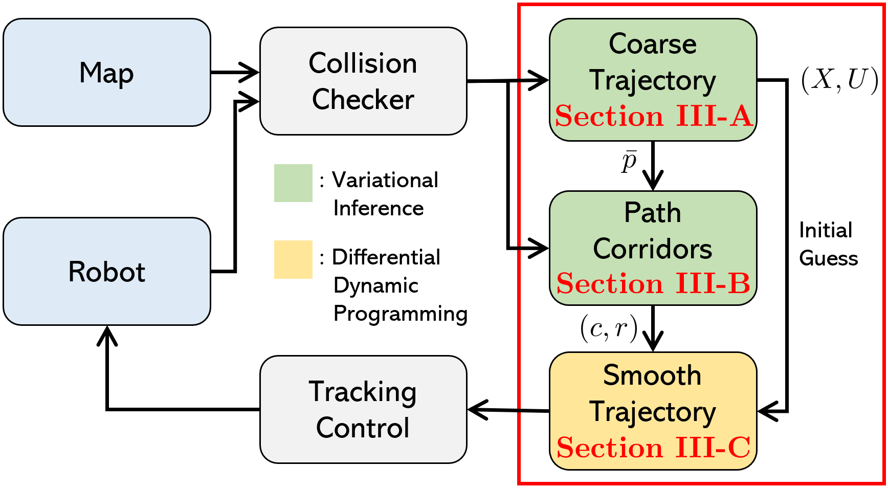
In this study, we propose a hybrid method of trajectory optimization by modularly incorporating sampling- and gradient-based methods. Fig. 1 depicts the structure of the proposed collision-free smooth path planning method. The hybrid method presented in this study generates a coarse trajectory and path corridors by using sampling-based optimization via variational inference (VI). Subsequently, a smooth trajectory is obtained by gradient-based optimization with a differential dynamic programming (DDP) scheme. It is assumed that a collision checker is available to indicate collision occurrence in a binary form, true or false.

Figure 1: Proposed method of collision-free smooth path planning. Contents in red box are subjects in this study.

VI refers to a class of optimization-based approaches of finding posterior distribution approximations of unknowns, and it makes Bayesian inference computationally efficient and scalable [5, 6]. Recently proposed model predictive path integral (MPPI) is a sampling-based planning method that uses a VI framework [7, 8]. Briefly, it samples random trajectories around a nominal trajectory and assigns weights to them in order of producing low costs. Subsequently, it updates the nominal trajectory with the weighted average. In this study, MPPI was used for generating a coarse trajectory for exploration while avoiding collision.

For smoothing the coarse trajectory with a gradient-based optimization, we introduced the concept of the path corridors, which is a well-known scheme reported in the literature [9, 4, 10, 11, 12]. Path corridors are collections of convex collision-free regions guiding a robot toward an aimed position. In this study, unlike the investigations mentioned above, a simple sampling-based optimization method was used to construct corridors.

To produce a smooth trajectory, a differential dynamic programming (DDP) framework can be applied in gradient-based optimization. DDP-based approaches, including iterative linear quadratic regulator, for nonlinear optimal control problems, have recently become commonly used in many applications of planning and nonlinear model predictive control for autonomous systems [13, 14]. DDP is based on Bellman’s principle of optimality and the necessary condition for optimal control problem. In addition, all functions defined in the optimal control problem are assumed to be smooth or at least twice continuously differentiable.

Because the original DDP approaches do not consider any constraints of the system state and inputs, many studies have been conducted to deal with constraints in DDP efficiently. The augmented Lagrangian (AL) method and the Karush-Kuhn-Tucker (KKT) condition were used in [15] and [16], respectively. In [14], a method combining the AL method with the KKT condition was proposed. The interior point differential dynamic programming (IPDDP) algorithm [17], employed in the present study, is based on the KKT condition. IPDDP, which is described in Section II-B, takes all Lagrangian and barrier terms into the so-called Q-function and solves a min-max problem.

The main contributions of this study are summarized as follows:

• We propose a hybrid path planning method that generates collision-free smooth trajectories by combining sampling-based trajectory optimization (MPPI) and gradient-based smooth optimization (IPDDP).

• We propose a method to construct collision-free convex path corridors by sampling-based optimization using VI.

• We present two numerical case studies for real-time path planning by which the effectiveness of the proposed method, MPPI-IPDDP, was demonstrated in the present research.

The remainder of this paper is organized as follows. Section II reviews sampling-based optimization by VI and IPDDP. Section III describes the proposed path planning method, called MPPI-IPDDP, which produces collision-free smooth trajectories. In Section IV, two-dimensional (2D) and three-dimensional (3D) case studies are presented to show the effectiveness of the proposed method. Section V concludes the paper and suggests directions for future studies.

II Preliminaries

II-A Sampling-based Optimization by Variational Inference

An optimization problem can be reconstructed as an inference problem, which can be solved by the VI method [18, 19]. To this end, in this study, a binary random variable $o$ indicating optimality was introduced where specifically, $p(o=1)$ is the probability of optimality. For brevity, we write it as $p(o)$.

We considered two different cases of VI for stochastic optimal control: VI for finite-dimensional optimization, in which the decision variable is a parameter vector, and VI for trajectory optimization, in which generating the optimal trajectory of a control system is considered.

II-A1 VI for Finite-dimensional Optimization

Let $\theta$ be a vector of decision variables. For VI corresponding to stochastic optimization or optimal control, the objective is to find the target distribution, $q^{*}$ defined as

$$q^{*}(\theta)=p(\theta\leavevmode\nobreak\ \!|\!\leavevmode\nobreak\ o)=\frac{p(o\leavevmode\nobreak\ \!|\leavevmode\nobreak\ \!\theta)p(\theta)}{\int p(o\leavevmode\nobreak\ \!|\leavevmode\nobreak\ \!\theta)p(\theta)d\theta}$$

Let $L(\theta)=p(o\leavevmode\nobreak\ \!|\!\leavevmode\nobreak\ \theta)$ be the likelihood function and $\tilde{q}^{*}$ be the empirical approximation of $q^{*}$ that is computed from samples $\{\theta_{1},\dots,\theta_{N}\}\sim p(\theta)$ drawn from prior $p(\theta)$. Thus, $\tilde{q}^{*}$ can be represented as

$$\tilde{q}^{*}(\theta)=\sum_{i=1}^{N}w_{i}\delta(\theta=\theta_{i})\enspace\!,\quad\!\!w_{i}=\frac{L(\theta_{i})}{\sum_{j=1}^{N}L(\theta_{j})}$$

where $\delta$ is the Dirac delta function and $N$ is the number of samples. Replacing $q^{*}$, $\tilde{q}^{*}$ is approximated using the forward Kullback-Leibler (KL) divergence as follows:

$$\pi^{*} =\underset{\pi}{\text{arg\,min}}\enspace\mathcal{D}_{\text{KL}}(\tilde{q}^{*}(\theta)\leavevmode\nobreak\ \!\|\!\leavevmode\nobreak\ \pi(\theta))$$

$$=\underset{\pi}{\text{argmax}}\enspace\mathbb{E}_{\theta\sim\tilde{q}^{*}(\theta)}\left[\log\pi(\theta)\right]\,.$$

If a normal distribution is chosen for parameterizing the policy, $\pi$, then a closed-form solution for the optimal policy, $\pi^{*}=\mathcal{N}(\mu,\Sigma)$, is obtained, where

$$\mu=\sum_{i=1}^{N}w_{i}\theta_{i}\enspace\!,\quad\!\!\Sigma=\sum_{i=1}^{N}w_{i}(\theta_{i}-\mu)(\theta_{i}-\mu)^{\top}$$ (1)

In this study, this VI-based stochastic optimization method was used for constructing collision-free convex path corridors, as described in Section III-B.

II-A2 VI for Trajectory Optimization

Let $\tau=(X,U)$ be a trajectory consisting of a sequence of controlled states $X=(x_{0},\dots,x_{T})$ and a sequence of control inputs $U=(u_{0},\dots,u_{T-1})$ over a finite time-horizon $T$. The objective is to find the target distribution, $q^{*}(\tau)=p(X\leavevmode\nobreak\ \!|\!\leavevmode\nobreak\ U)q^{*}(U)$, where $p(X\leavevmode\nobreak\ \!|\!\leavevmode\nobreak\ U)$ represents stochastic dynamics as follows:

$$q^{*}(\tau) =\underset{q(\tau)}{\text{arg\,min}}\enspace\mathcal{D}_{\text{KL}}(q(\tau)\,\|\,p(\tau\leavevmode\nobreak\ \!|\leavevmode\nobreak\ \!o))$$

$$=\underset{q(\tau)}{\text{arg\,min}}\enspace\!-\mathbb{E}_{\tau\sim q(\tau)}\left[\log p(o\leavevmode\nobreak\ \!|\!\leavevmode\nobreak\ \tau)\right]+\mathcal{D}_{\text{KL}}(q(U)\leavevmode\nobreak\ \!\|\!\leavevmode\nobreak\ p(U))\,.$$

Let $L(U)=\mathbb{E}_{X\sim p(X\leavevmode\nobreak\ \!|\!\leavevmode\nobreak\ U)}\left[\log p(o\leavevmode\nobreak\ \!|\!\leavevmode\nobreak\ \tau)\right]$. Thus, $q^{*}(\tau)$ can be rewritten as

$$q^{*}(U)=\underset{q(U)}{\text{arg\,min}} -\mathbb{E}_{U\sim q(U)}\left[L(U)\right]+\mathcal{D}_{\text{KL}}(q(U)\leavevmode\nobreak\ \!\|\!\leavevmode\nobreak\ p(U))$$

s.t. $$\int q(U)dU=1\,.$$

The closed-form solution for the above optimization is expressed as

$$q^{*}(U)=\frac{\exp(L(U))p(U)}{\int\exp(L(U))p(U)dU}$$

Let $\tilde{q}^{*}$ be the empirical distribution of $q^{*}$ approximated with samples $\{U_{1},\dots,U_{N}\}\sim p(U)$ drawn from prior $p(U)$. Thus, $\tilde{q}^{*}$ can be represented as

$$\tilde{q}^{*}(U)=\sum_{i=1}^{N}w_{i}\delta(U=U_{i})\enspace\!,\quad\!\!w_{i}=\frac{\exp(L(U_{i}))}{\sum_{j=1}^{N}\exp(L(U_{j}))}$$

Replacing $q$, $\tilde{q}^{*}$ is approximated with the forward KL divergence.

$$\pi^{*}=\underset{\pi}{\text{arg\,min}}\enspace\mathcal{D}_{\text{KL}}(\tilde{q}^{*}(U)\leavevmode\nobreak\ \!\|\!\leavevmode\nobreak\ \pi(U))$$

If a normal distribution is chosen for $\pi$, then a closed form solution of $\pi^{*}=\mathcal{N}(\mu,\Sigma)$ is obtained, where

$$\mu=\sum_{i=1}^{N}w_{i}U_{i}\enspace\!,\quad\!\!\Sigma=\sum_{i=1}^{N}w_{i}(U_{i}-\mu)(U_{i}-\mu)^{\top}$$ (2)

In this study, this VI-based trajectory optimization method was used in MPPI [7, 8] to generate a locally optimal trajectory, as presented in Section III-A.

II-A3 Additional Notes

One of the most common choices for the likelihood function is $p(o\leavevmode\nobreak\ \!|\!\leavevmode\nobreak\ \cdot)=\exp(-\gamma J(\cdot))$, where $J(\cdot)$ is the cost function and $\gamma>0$ is known as the inverse temperature. Using this likelihood function, weight $w_{i}$, as discussed in Sections II-A1 and II-A2 can be interpreted as the likelihood ratio corresponding to the sampled candidate, $\theta_{i}$ or $U_{i}$, respectively. Specifically, a low value of $J$ implies a high likelihood of optimality at an exponential rate.

Because this sampling-based optimization scheme is an iterative method, the distribution, $\pi$, affects the prior, $p$, at the next iteration; therefore, $\pi$ eventually reaches a locally optimal point. In this study, we considered normal distributions for the prior and posterior, and only propagated the mean, $\mu$, and used a fixed covariance $\Sigma$ without empirical adaptation, as expressed (1) and (2).

In [20], the Stein variational gradient descent (SVGD) method was proposed to directly approximate a target distribution $q^{*}$ by the reverse KL divergence, without using an empirical distribution $\tilde{q}^{*}$. In addition, it can deal with complex multi-modal distributions and achieve more exploration; consequently, a global optimum is more probable to be found. Although SVGD can be used as in [21], in this study, an empirical distribution and the forward KL divergence were employed for convenience.

II-B Interior Point Differential Dynamic Programming

IPDDP introduced in [17] can be used to solve a standard discrete-time optimal control problem (OCP) expressed as

$$\underset{u_{0:T-1}}{\text{minimize}} l_{f}(x_{T})+\sum_{t=0}^{T-1}l_{t}(x_{t},u_{t})$$ (3)

subject to $$x_{t+1}=f_{t}(x_{t},u_{t}),\,x_{0}=x_{\rm init}$$

$$g_{t}(x_{t},u_{t})\leq 0$$

where variables $x_{t}\in\mathbb{R}^{n}$ and $u_{t}\in\mathbb{R}^{m}$ are the system state and the control input vector at time step $t$, respectively, and $x_{\rm init}$ is the initial condition of the control system. Let the decision vector be denoted as $U:=u_{0:T-1}=[u_{0}^{\top},u_{1}^{\top},\cdots,u_{T-1}^{\top}]^{\top}\in\mathbb{R}^{nT}$, which is a concatenation of sequential control inputs over a time horizon $T$. Real-valued functions $l_{f}:\mathbb{R}^{n}\rightarrow\mathbb{R}$ and $l_{t}:\mathbb{R}^{n}\times\mathbb{R}^{m}\rightarrow\mathbb{R}$ are the final and stage cost functions, respectively, and $f_{t}:\mathbb{R}^{n}\times\mathbb{R}^{m}\rightarrow\mathbb{R}^{n}$ defines the controlled state transitions. Vector-valued function $g_{t}:\mathbb{R}^{n}\times\mathbb{R}^{m}\rightarrow\mathbb{R}^{k}$ defines the inequality constraints, where $k$ denotes the number of constraints. All functions defined in (3) are assumed to be twice continuously differentiable.

In dynamic programming, the OCP (3) can be converted into Bellman’s equation form at time $t$ with a given state $x_{t}$ as follows:

$$V_{t}(x_{t})=\underset{u_{t},s_{t}}{\text{min}} l_{t}(x_{t},u_{t})+V_{t+1}(f_{t}(x_{t},u_{t}))$$

subject to $$g_{t}(x_{t},u_{t})+s_{t}=0$$

$$s_{t}\geq 0$$

where $V_{t+1}$ is a value function for the next state and $s_{t}=[s^{1},\dots,s^{k}]^{\top}_{t}\in\mathbb{R}^{k}$ are slack variables. At the final stage, the value function is defined as $V_{T}(x_{T})=l_{f}(x_{T})$. For notational convenience, index $t$ is not shown in the remainder of this section. The relaxed Lagrangian with the log-barrier terms of $s$ is defined by the following $Q$-function:

$$Q(x,u,s,y) =l(x,u)+V^{\prime}(f(x,u))$$

$$+y^{\top}(c(x,u)+s)-\mu\sum_{i=1}^{k}\log s^{i}$$

where $\mu>0$ is the barrier parameter and $y$ is the Lagrangian multiplier. The relaxed value function, $V(x)$, is defined by a saddle point of the $Q$-function as follows:

$$V(x)=\underset{u,s}{\min}\ \underset{y}{\max}\enspace Q(x,u,s,y)$$

II-B1 Backward Pass

As in the standard DDP scheme, $Q$ is perturbed up to the quadratic terms at the current nominal points:

$$\delta Q =\begin{bmatrix}Q_{x}\\ Q_{u}\\ Q_{s}\\ Q_{y}\end{bmatrix}^{\!\!\top}\!\!\!\begin{bmatrix}\delta x\\ \delta u\\ \delta s\\ \delta y\end{bmatrix}\!+{1\over 2}\!\begin{bmatrix}\delta x\\ \delta u\\ \delta s\\ \delta y\end{bmatrix}^{\!\!\top}\!\!\!\left[\begin{array}[]{@{\,}c@{\,\,}c@{\,\,}c@{\,\,}c@{\,}}Q_{xx}&Q_{xu}&Q_{xs}&Q_{xy}\\ Q_{ux}&Q_{uu}&Q_{us}&Q_{uy}\\ Q_{sx}&Q_{su}&Q_{ss}&Q_{sy}\\ Q_{yx}&Q_{yu}&Q_{ys}&Q_{yy}\\ \end{array}\right]\!\begin{bmatrix}\delta x\\ \delta u\\ \delta s\\ \delta y\end{bmatrix}$$ (8)

$$=Q_{x}^{\top}\delta x+{1\over 2}\delta x^{\top}Q_{xx}\delta x$$ (9)

$$\quad+\delta x^{\top}\!\begin{bmatrix}Q_{xu}&\!\!\!\!0&\!\!\!\!Q_{xy}\end{bmatrix}\!\begin{bmatrix}\delta u\\ \delta s\\ \delta y\end{bmatrix}+\begin{bmatrix}Q_{u}\\ y-\mu S^{-1}e\\ Q_{y}\end{bmatrix}^{\!\!\top}\!\!\!\begin{bmatrix}\delta u\\ \delta s\\ \delta y\end{bmatrix}$$

$$\quad+{1\over 2}\begin{bmatrix}\delta u\\ \delta s\\ \delta y\end{bmatrix}^{\!\!\top}\!\!\!\left[\begin{array}[]{@{\,}c@{\,\,}c@{\,\,}c@{\,}}Q_{uu}&0&Q_{uy}\\ 0&\mu S^{-2}&I\\ Q_{yu}&I&0\\ \end{array}\right]\!\!\begin{bmatrix}\delta u\\ \delta s\\ \delta y\end{bmatrix}$$ (13)

where $e\in\mathbb{R}^{k}$ is an all-ones vector and $S:=\text{diag}(s)\in\mathbb{R}^{k\times k}$ is a diagonal matrix associated with vector $s\in\mathbb{R}^{k}$. By setting $\delta s^{\top}(\mu S^{-2})\delta s=\delta s^{\top}(S^{-1}Y)\delta s$, where $Y:=\text{diag}(y)$, the step direction that satisfies the extremum condition corresponding to the first-order optimality is determined using the following primal-dual KKT system as follows:

$$\left[\begin{array}[]{@{\,}c@{\,\,\,}c@{\,\,\,}c@{\,}}Q_{uu}&0&Q_{uy}\\ 0&Y&S\\ Q_{yu}&I&0\\ \end{array}\right]\!\!\begin{bmatrix}\delta u\\ \delta s\\ \delta y\end{bmatrix}=-\begin{bmatrix}Q_{ux}\\ 0\\ Q_{yx}\end{bmatrix}\delta x-\begin{bmatrix}Q_{u}\\ Sy-\mu e\\ Q_{y}\end{bmatrix}$$ (14)

Solving the KKT system expressed in (14) for $\delta u$, $\delta s$, and $\delta y$, yields

$$\delta u=K_{u}\delta x+d_{u}\enspace\!,\quad\!\!\delta s=K_{s}\delta x+d_{s}\enspace\!,\quad\!\!\delta y=K_{y}\delta x+d_{y}$$

where the coefficient matrices and the vectors are defined as

$$K_{u}=-\tilde{Q}_{uu}^{-1}\tilde{Q}_{ux}\,, d_{u}=-\tilde{Q}_{uu}^{-1}\tilde{Q}_{u}\,,$$

$$K_{s}=-(Q_{yx}+Q_{yu}K_{u})\,, d_{s}=-(r_{p}+Q_{yu}d_{u})\,,$$ (15)

$$K_{y}=S^{-1}Y(Q_{yx}+Q_{yu}K_{u})\,, d_{y}=S^{-1}(r+YQ_{yu}d_{u})$$

and the intermediate parameters and vectors are

$$\tilde{Q}_{u}=Q_{u}+Q_{uy}S^{-1}r\,,\, r=Yr_{p}-r_{d}\,,$$

$$\tilde{Q}_{uu}=Q_{uu}+Q_{uy}S^{-1}YQ_{yu}\,,\, r_{p}=Q_{y}\,,$$ (16)

$$\tilde{Q}_{ux}=Q_{ux}+Q_{uy}S^{-1}YQ_{yx}\,,\, r_{d}=Sy-\mu e\,.$$

Above, $r_{p}$ and $r_{d}$ are the primal and dual residuals, respectively. The KKT variables, $\delta s$ and $\delta y$, can be rewritten as

$$\delta s =S^{-1}YQ_{yx}\delta x+S^{-1}YQ_{yu}\delta u+S^{-1}r\,,$$

$$\delta y =-Q_{yx}\delta x-Q_{yu}\delta u-r_{p}\,.$$

Substituting the above expressions of $\delta s$ and $\delta y$ into the quadratic form, $\delta Q$, in (9) and setting $\delta s^{\top}(\mu S^{-2})\delta s=\delta s^{\top}(S^{-1}Y)\delta s$ yield another representation for the perturbed quadratic form as follows:

$$\delta Q= {1\over 2}r_{p}^{\top}S^{-1}Yr_{p}-r_{d}^{\top}S^{-1}r_{p}+\begin{bmatrix}\tilde{Q}_{x}\\ \tilde{Q}_{u}\end{bmatrix}^{\top}\begin{bmatrix}\delta x\\ \delta u\end{bmatrix}$$

$$+{1\over 2}\begin{bmatrix}\delta x\\ \delta u\end{bmatrix}^{\top}\begin{bmatrix}\tilde{Q}_{xx}&\tilde{Q}_{ux}^{\top}\\ \tilde{Q}_{ux}&\tilde{Q}_{uu}\end{bmatrix}\begin{bmatrix}\delta x\\ \delta u\end{bmatrix}$$

where $\tilde{Q}_{x}=Q_{x}+Q_{xy}S^{-1}r$ and $\tilde{Q}_{xx}=Q_{xx}+Q_{xy}S^{-1}YQ_{yx}$.

Finally, the perturbed value function is obtained as follows:

$$\delta V=\underset{\delta u,\delta s}{\min}\underset{\delta y}{\max}\enspace\delta Q=\Delta V+V_{x}^{\top}\delta x+{1\over 2}\delta x^{\top}V_{xx}\delta x$$

where the coefficients are

$$\Delta V =\tilde{Q}^{\top}_{u}d_{u}+{1\over 2}d_{u}^{\top}\tilde{Q}_{uu}d_{u}+{1\over 2}r_{p}^{\top}S^{-1}Yr_{p}-r_{d}^{\top}S^{-1}r_{p}\,,$$

$$V_{x} =\tilde{Q}_{x}+K_{u}^{\top}\tilde{Q}_{u}+\tilde{Q}_{ux}^{\top}d_{u}+K_{u}^{\top}\tilde{Q}_{uu}d_{u}\,,$$

$$V_{xx} =\tilde{Q}_{x}x+K_{u}^{\top}\tilde{Q}_{ux}+\tilde{Q}_{ux}^{\top}K_{u}+K_{u}^{\top}\tilde{Q}_{uu}K_{u}\,.$$

This perturbed value function, $\delta V$, is recursively used for $\delta V^{\prime}$ in the next backward step.

II-B2 Forward Pass

After calculating the perturbations in the backward pass, the nominal points are updated as follows: $u\leftarrow u+\alpha\delta u$, $s\leftarrow s+\alpha\delta s$, and $y\leftarrow y+\alpha\delta y$, where $\alpha\in(0,1]$ is the step size. In IPDDP, $\alpha$ is determined using the filter line-search method [1]. While reducing the step size, $\alpha$, starting from $1$, the filter line-search method accepts those updates that reduce either the cost or constraint violations. If no $\alpha$ is found acceptable, the forward pass is terminated for failure.

II-B3 Convergence

The barrier parameter, $\mu$, is monotonically decreased whenever the local convergence to the central path is achieved. The criterion for local convergence is $\max(\|Q_{u}\|_{\infty},\|r_{p}\|_{\infty},\|r_{d}\|_{\infty})<\kappa\mu$, where $\kappa>1$. The global convergence agrees with the sufficiently small $\mu$.

II-B4 Regularization

To guarantee that $\tilde{Q}_{uu}^{-1}$ is invertible in (II-B1), regularization parameter $\rho\geq 0$ is added: $Q_{uu}\leftarrow Q_{uu}+\rho I_{m}$. $\rho$ increases when it is not invertible or failure occurs in the forward pass. If $\rho$ reaches some upper bound $\rho_{\max}$, IPDDP is terminated for failure.

III Collision-free Smooth Trajectory Generation

This study considers the following OCP associated with trajectory optimization for path planning:

$$\underset{u_{0:T-1}}{\text{minimize}} l_{f}(x_{T})+\sum_{t=0}^{T-1}l(x_{t},u_{t})$$ (17)

subject to $$x_{t+1}=f(x_{t},u_{t}),\,x_{0}=x_{\rm init}$$

$$g(x_{t})\leq 0,\ h(u_{t})\leq 0$$

$$p_{t}\notin\mathcal{O}$$

where $p_{t}\in x_{t}$ is the position of a robot and $\mathcal{O}$ is the set of positions occupied by obstacles. Different from (3), the joint constraints on states and controls are decoupled. The proposed algorithm for solving (17) has three steps: searching for a feasible coarse trajectory using MPPI, constructing path corridors, and smoothing the coarse trajectory by IPDDP.

III-A Model Predictive Path Integral

First, a coarse trajectory using MPPI is generated. The cost function, $J$, is defined as

$$J(U)=l_{f}(x_{T})+\sum_{t=0}^{T-1}l(x_{t},u_{t})+\mathcal{I}^{\text{\scriptsize MPPI}}(x_{t})$$ (18)

where the indicator function for collision avoidance is defined as

$$\mathcal{I}^{\text{\scriptsize MPPI}}(x_{t})=\begin{cases}\infty,&\text{if\enspace}p_{t}\in\mathcal{O}\text{\enspace or\enspace}g(x_{t})>0\\ 0,&\text{otherwise}\end{cases}$$

and the sequence of states $x_{0:T}$ is determined by the initial state, $x_{0}=x_{\rm init}$, dynamics $x_{t+1}=f(x_{t},u_{t})$, and controls $U$.

To satisfy the control constraints in (17), the samples of controls, $U_{i}$, are projected onto the constraint set, i.e. $U_{i}\leftarrow\Pi(U_{i})$, where $\Pi$ is a projection operator applied to the feasible set of controls $\{u_{0:T-1}\in\mathbb{R}^{mT}\,|\,h(u_{i})\leq 0\ \text{for all $i$}\}$.

Using the method described in Section II-A2, locally optimal controls and corresponding states are obtained. Let $\bar{p}_{0:T}$ be the resulting position of a robot obtained by MPPI.

III-B Path Corridors

To construct corridors around a path $\bar{p}_{0:T}$, the following optimization problem is considered:

$$\underset{c,r}{\text{minimize}} J(c,r)=\lambda_{c}\|c-\bar{p}\|_{2}-\lambda_{r}r+\mathcal{I}^{\text{\scriptsize PC}}(c,r)$$ (19)

subject to $$\|c-\bar{p}\|_{2}\leq r$$

$$0\leq r\leq r_{\rm max}$$

where the indicator function for a radial collision-free corridor is defined as

$$\mathcal{I}^{\text{\scriptsize PC}}(c,r) =\begin{cases}\infty,&\text{if\enspace}\mathcal{B}_{r}(c)\bigcap\mathcal{O}\neq\emptyset\\ 0,&\text{otherwise}\end{cases}$$

$$\mathcal{B}_{r}(c) =\{p\ |\ \|p-c\|_{2}\leq r\}\,.$$

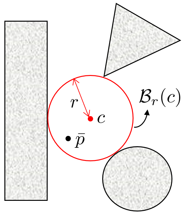
Parameters $\lambda_{c},\lambda_{r}>0$ are the weights and $r_{\max}$ is the maximum value of $r$. Although the shape of the corridors can be arbitrary, we selected a Euclidean ball $\mathcal{B}_{r}(c)$ represented by two variables: center $c$ and radius $r$. The problem as expressed in (19) is designed to enlarge the ball and ensure the center, $c$, close to $\bar{p}$ while containing $\bar{p}$ inside the ball without intersection with obstacles (see Fig. 2). If there are no obstacles around $\bar{p}$, the optimal solutions are $c=\bar{p}$ and $r=r_{\max}$.

The method described in Section II-A1 was used with $\theta=[c^{\top},r]^{\top}$ to solve the optimization problem in (19) at each stage of the path planning to compute a sequence of collision-free corridors, which are represented by $C=[c_{0}^{\top},\dots,c_{T-1}^{\top}]^{\top}$ and $R=[r_{0},\dots,r_{T-1}]^{\top}$. As in MPPI, the constraints on $c,r$ in (19) can be met by projection.

(a) Maximally inflated path corridor

(b) Inflation process

Figure 2: Schematics for collision-free path corridors.

III-C Trajectory Smoothing

In the final step of the proposed trajectory optimization for path planning, the following OCP is considered for smoothing the coarse trajectory generated by MPPI:

$$\underset{u_{0:T-1}}{\text{minimize}} l_{f}(x_{T})+\sum_{t=0}^{T-1}l(x_{t},u_{t})+\|p_{t}-c_{t}\|^{2}_{Q}$$ (20)

subject to $$x_{t+1}=f_{t}(x_{t},u_{t}),\,x_{0}=x_{\rm init}$$

$$g_{t}(x_{t})\leq 0,\ h_{t}(u_{t})\leq 0$$

$$\|p_{t}-c_{t}\|_{2}\leq r_{t}$$

where $p_{t}\in x_{t}$ is, again, the position of a robot, $(c_{t},r_{t})$ are the center and radius of the path corridor computed using (19), and $Q$ is a weight matrix penalizing the deviations from the center of a corridor. The constraint in the last row of (20) is included to ensure the robot remains inside the collision-free corridors.

IPDDP introduced in Section II-B was adopted to solve (20) and obtain a smooth trajectory. At the time, the coarse trajectory from the MPPI can be used for the initial guess, i.e., a warm start for local optimization; this can considerably accelerate the convergence rate of IPDDP.

III-D Algorithms

Algorithm 1 summarizes the proposed trajectory optimization method, MPPI-IPDDP, for generating collision-free smooth trajectories. The algorithm consists of three subroutines. First, MPPI uses a derivate-free VI to search a dynamically feasible but coarse trajectory. Second, Corridor also uses a derivate-free VI to construct collision-free circular corridors around the coarse trajectory. Finally, IPDDP employs a recursive method to smooth the coarse trajectory within the corridors. As demonstrated in the supplementary video available at https://youtu.be/-oUAt5sd9Bk, the proposed MPPI-DDP is verified to be capable of online replanning.

Algorithm 1 ${\tt MPPI\mbox{-}IPDDP}$

1:Input: initial state $x_{0}$, collision checker

2:Output: locally optimal controls $U^{*}$

3:Initialize: controls $U$

4:while not terminated do

5:    $U\leftarrow{\tt MPPI}(x_{0},U)$

6:    for $t=0,1,\dots,T-1$ do

7:         $x_{t+1}\leftarrow f(x_{t},u_{t})$

8:    end for

9:    $(C,R)\leftarrow{\tt Corridor}(X)$ $\triangleright$ $X=[x^{\top}_{0},\dots,x^{\top}_{T}]^{\top}$

10:    $U\leftarrow{\tt IPDDP}(X,U,C,R)$ $\triangleright$ (20)

11:end while

Algorithm 2 ${\tt MPPI}$

1:for $i=1,\dots,N_{u}$ do

2:    $\hat{U}_{i}\leftarrow\Pi_{u}(U+\varepsilon_{i})\ ,\quad\varepsilon_{i}\sim\mathcal{N}(0,\Sigma_{u})$

3:    $J_{i}\leftarrow{\tt cost}(x_{0},\hat{U}_{i})$ $\triangleright$ (18)

4:end for

5:$\bar{J}\leftarrow\min_{i}J_{i}$

6:for $i=1,\dots,N_{u}$ do

7:    $J_{i}\leftarrow J_{i}-\bar{J}$

8:    $w_{i}\leftarrow\exp(-\gamma_{u}J_{i})$

9:end for

10:$\bar{w}\leftarrow\sum_{i=1}^{N_{u}}w_{i}$

11:$U\leftarrow\sum_{i=1}^{N_{u}}(w_{i}/\bar{w})\hat{U}_{i}$

12:$U\leftarrow\Pi_{u}(U)$

Algorithm 3 ${\tt Corridor}$

1:$\bar{p}_{0:T}\leftarrow\text{extract positions from $X$}$

2:$c_{t}\leftarrow\bar{p}_{t}\enspace\text{for every $t=0,\dots,T-1$}$

3:$r_{t}\leftarrow 0\enspace\text{for every $t=0,\dots,T-1$}$

4:$Z\leftarrow(C,R)=[c^{\top}_{0},r_{0},c^{\top}_{1},r_{1},\dots,c^{\top}_{T-1},r_{T-1}]^{\top}$

5:while not sufficiently inflated do

6:    for $i=1,\dots,N_{z}$ do

7:         $\hat{Z}_{i}\leftarrow\Pi_{z}(Z+\varepsilon_{i})\ ,\quad\varepsilon_{i}\sim\mathcal{N}(0,\Sigma_{z})$

8:         $J_{i}\leftarrow{\tt cost}(\hat{Z}_{i})$ $\triangleright$ (19)

9:    end for

10:    $\bar{J}\leftarrow\min_{i}J_{i}$

11:    for $i=1,\dots,N_{z}$ do

12:         $J_{i}\leftarrow J_{i}-\bar{J}$

13:         $w_{i}\leftarrow\exp(-\gamma_{z}J_{i})$

14:    end for

15:    $\bar{w}\leftarrow\sum_{i=1}^{N_{z}}w_{i}$

16:    $Z\leftarrow\sum_{i=1}^{N_{z}}(w_{i}/\bar{w})\hat{Z}_{i}$

17:    $Z\leftarrow\Pi_{z}(Z)$

18:end while

19:$(C,R)\leftarrow Z$  (unpacking)

Algorithm 4 ${\tt IPDDP}$

1:while not converged globally and not max iteration do

2:    evaluate all derivatives needed;

3:    try backwardpass; $\triangleright$ Section II-B1

4:    try forwardpass; $\triangleright$ Section II-B2

5:    if any failure occurs then $\triangleright$ Section II-B4

6:         increase regularization parameter $\rho$;

7:         if $\rho>\rho_{\max}$ then

8:             break; $\triangleright$ Solve failed

9:         end if

10:         continue;

11:    else

12:         decrease regularization parameter $\rho$;

13:         update nominal trajectory;

14:    end if

15:    if locally converged then $\triangleright$ Section II-B3

16:         decrease barrier parameter $\mu$;

17:         reinitialize filter;

18:    end if

19:end while

IV Case Studies

In this section, we present two simulation results of trajectory optimization conducted to demonstrate the effectiveness of the proposed MPPI-IPDDP. The first case is of a wheeled mobile robot, and the second case considers a point-mass quadrotor.

IV-A Wheeled Mobile Robot

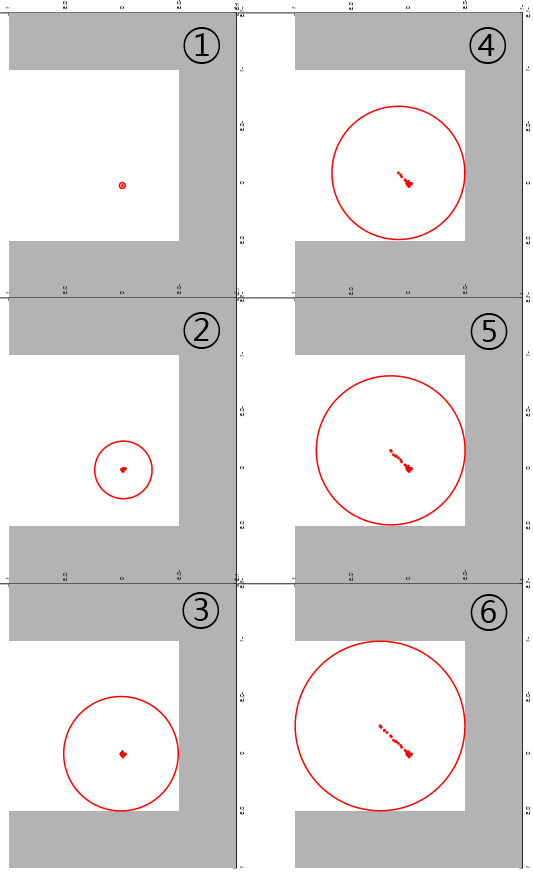
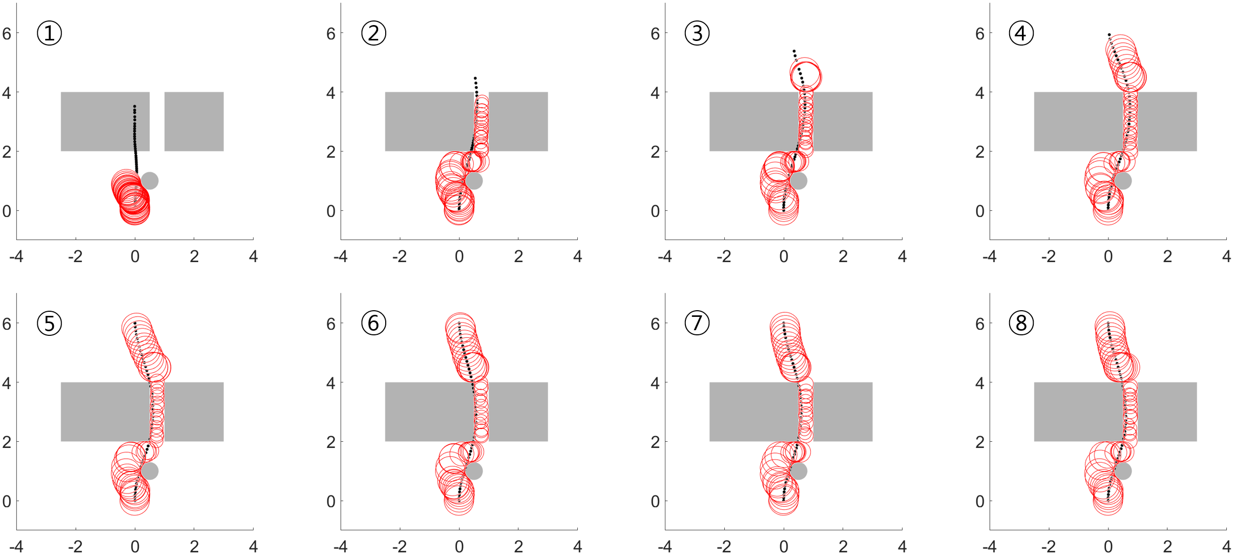
Figure 3: Iterations of MPPI-IPDDP algorithm for generating collision-free path from $(0,0)$ to $(0,6)$. Black dots mark positions of robot, red circles represent the path corridors, and gray color represents obstacles. Early part of iterations shows that constraint violation (black dots are not in corridors) because IPDDP is terminated by maximum iteration limit. However, finally, MPPI-IPDDP algorithm finds optimal collision-free trajectory.

(a) Coarse controls by MPPI

(b) Smooth controls by IPDDP

Figure 4: Comparison of control inputs obtained by MPPI and IPDDP.

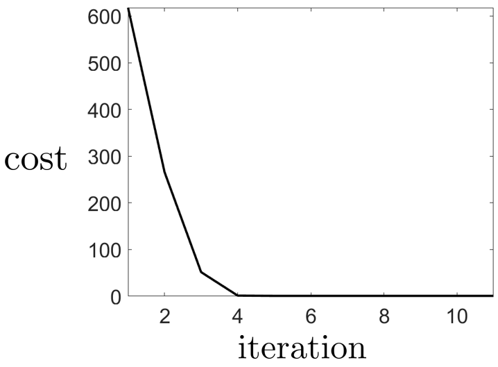
(a) Cost of trajectory reduces over iterations.

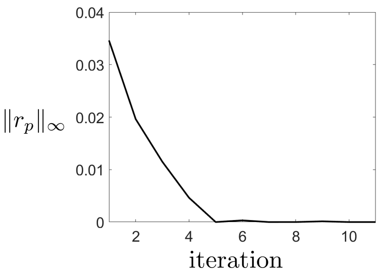
(b) Maximum value of primal residual approaches zero, indicating that constraints are satisfied.

Figure 5: Cost reduction and convergence rate over MPPI-IPDDP iterations.

For an example of 2D path planning, a scenario in which a differential wheeled robot arrives at a given target pose without collision was considered. The kinematic model of the robot is defined as

$$x_{t+1} =x_{t}+v_{t}\cos(\theta_{t})\Delta t$$

$$y_{t+1} =y_{t}+v_{t}\sin(\theta_{t})\Delta t$$

$$\theta_{t+1} =\theta_{t}+w_{t}\Delta t$$

where $(x_{t},y_{t})\in\mathbb{R}$ are the positions on the x- and y-axis respectively; $\theta_{t}\in\mathbb{R}$ is the angle of orientation; $v_{t},w_{t}\in\mathbb{R}$ are the velocity and angular velocity, respectively; and $\Delta t$ is the time interval. Vectors $[x_{t},y_{t},\theta_{t}]^{\top}$ and $[v_{t},w_{t}]^{\top}$ are the states and the controls, respectively. We set the initial states as $[0,0,\pi/2]^{\top}$ and the sampling time interval as $\Delta t=0.1$.

The constraints of the corresponding OCP for trajectory generation are defined as

$$0\leq v_{t}\leq 1.5\ ,\ |w_{t}|\leq 1.5\ ,\ (x_{t},y_{t})\notin\mathcal{O}$$

where $\mathcal{O}$ is the set of obstacles shown in Fig. 3 in gray. The cost functions of the corresponding OCP for trajectory generation are defined as

$$l_{f} =300(x_{T}^{2}+(y_{T}-6)^{2}+(\theta_{T}-\pi/2)^{2})$$

$$l =0.01(v_{t}^{2}+w_{t}^{2})$$

where $[0,6,\pi/2]^{\top}$ is the target pose. The parameters for the MPPI-IPDDP method are listed in Table I.

Table I: Parameters for trajectory optimization of wheeled mobile robot, as described in Section IV-A.

Parameter	Value	Parameter	Value
$\lambda_{c}$	20	$\lambda_{r}$	35
$r_{\text{max}}$	0.5	$T$	50
$\gamma_{z}$	1000	$\gamma_{u}$	100
$N_{u}$	5000	$\Sigma_{u}$	$\text{diag}([0.25,0.25])$
$N_{z}$	3000	$\Sigma_{z}$	$\text{diag}([0.3,0.3,0.08])$
$Q$	$0.001I_{3}$

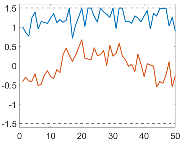
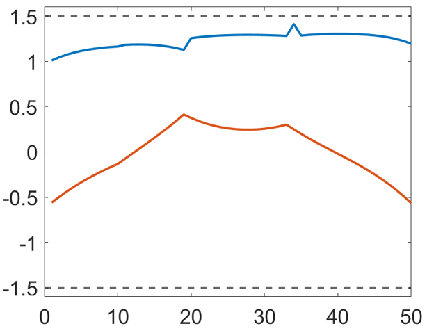
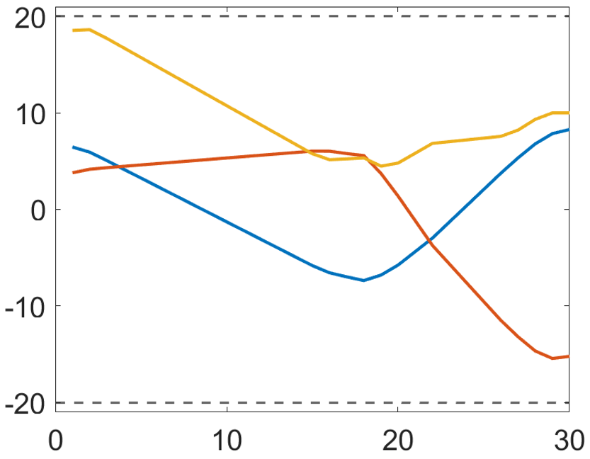
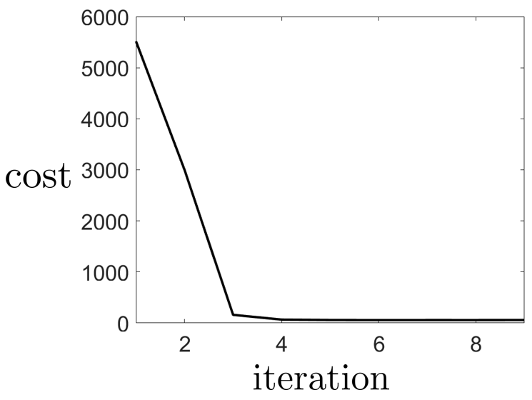
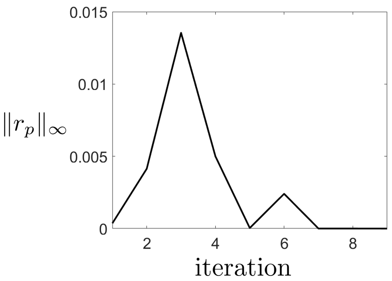
Fig. 3 shows the processing results of generating a smooth trajectory. In Fig. 5, the zigzag controls obtained by MPPI and the smoother ones by IPDDP are compared. Fig. 5 shows that the cost and constraint violations reduce with increasing MPPI-IPDDP iterations.

IV-B Quadrotor Without Attitude

Table II: Parameters for trajectory optimization of quadrator, as described in Section IV-B.

Parameter	Value	Parameter	Value
$\lambda_{c}$	20	$\lambda_{r}$	35
$r_{\text{max}}$	0.5	$T$	30
$\gamma_{z}$	1000	$\gamma_{u}$	100
$N_{u}$	8000	$\Sigma_{u}$	$\text{diag}([1.5,1.5,1.5])$
$N_{z}$	5000	$\Sigma_{z}$	$\text{diag}([0.3,0.3,0.3,0.08])$
$Q$	$0.001I_{3}$

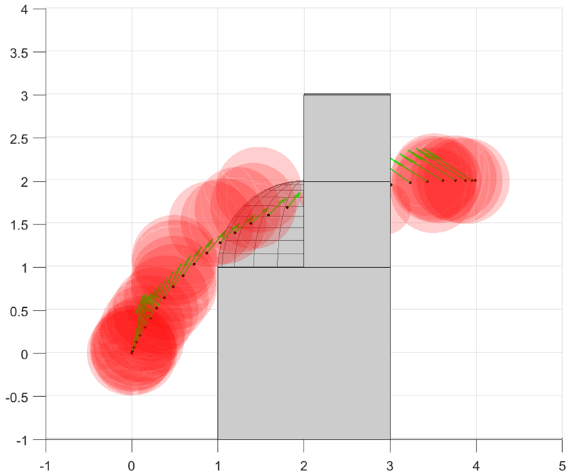
Figure 6: Iterations for generating path from $(0,0,0)$ to $(0,4,2)$ by MPPI-IPDDP. Black dots are positions of quadrotor, red spheres are path corridors, and gray color represents obstacles. Optimal trajectory passes through small hole and reaches destination.

Figure 7: Side view of generated trajectory. Green arrows represent directions of acceleration.

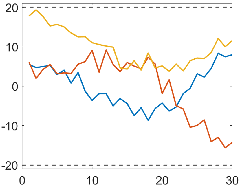
(a) Coarse controls by MPPI

(b) Smooth controls by IPDDP

Figure 8: Comparison of control inputs obtained by MPPI and IPDDP.

(a) Cost of trajectory reduces over iterations.

(b) Maximum value of primal residual approaches zero, indicating that constraints are satisfied.

Figure 9: Cost reduction and convergence rate over MPPI-IPDDP iterations.

As an example of 3D path planning, a scenario in which a quadrotor arrives at a given target position without collision was considered. it was assumed that the quadrotor can be modeled as a point mass. The kinematics of the quadrotor is given by

$$x_{t+1} =x_{t}+v_{t}\Delta t$$

$$v_{t+1} =v_{t}+(a_{t}-ge_{3})\Delta t$$

where $x_{t}\in\mathbb{R}^{3}$ and $v_{t}\in\mathbb{R}^{3}$ are the position and the velocity, respectively, $a_{t}\in\mathbb{R}^{3}$ is the acceleration, $g=9.81$ is the gravitational acceleration, and $e_{3}=[0,0,1]^{\top}$ is the vector of z-axis. $[x_{t}^{\top},v_{t}^{\top}]^{\top}$ and $a_{t}$ are the states and the controls, respectively. The initial state is set as $[0,0,0,0,0,0]^{\top}$, and $\Delta t=0.05$.

The constraints of the corresponding OCP for trajectory generation are defined as

$$\|a_{t}\|_{2}\leq 20\,,\ \|a_{t}\|_{2}\cos(60^{\circ})\leq e_{3}^{\top}a_{t}\,,\ \mbox{and}\ x_{t}\notin\mathcal{O}$$

where the first two constraints represent that the acceleration of the quadrotor must be inside a cone and $\mathcal{O}$ is the set of obstacles shown in Fig. 7 in gray. When projections are performed to satisfy the conic constraint, the following projection operator was applied for obtaining a second-order cone:

$$\Pi(u)=\begin{cases}\vspace{-.75mm}0&\text{if\enspace}\|v\|_{2}\leq-s\\[5.69054pt] u&\text{if\enspace}\|v\|_{2}\leq s\\ {1\over 2}\!\left(1+{s\over\|v\|_{2}}\right)\!\begin{bmatrix}v\\ \|v\|_{2}\end{bmatrix}&\text{if\enspace}\|v\|_{2}>|s|\end{cases}\vspace{-.25mm}$$

for $u=[v^{\top}s]^{\top}$, where $v$ and $s$ are a vector of a compatible dimension and a scalar, respectively. The cost functions of the corresponding OCP for trajectory generation are defined as

$$l_{f} =500(\|x_{T}-[0,4,2]^{\top}\|_{2}^{2}+\|v_{T}\|_{2}^{2})$$

$$l =0.01\|a_{t}\|_{2}^{2}$$

where $[0,4,2]^{\top}$ is the target position. The parameters for the MPPI-IPDDP method are listed in Table II.

Fig. 6 shows the processing results of generating a smooth trajectory. Fig. 9 compares the noisy controls obtained by MPPI and the smooth ones obtained by IPDDP. Fig. 9 shows that the cost and constraint violations reduce with increasing MPPI-IPDDP iterations.

V Conclusion

In this study, we established a new optimization-based hybrid local path planning method, MPPI-IPDDP, to generate a collision-free smooth optimal trajectory for path planning. Based on two case studies of ground and aerial robot path planning, we demonstrated the effectiveness of the proposed MPPI-IPDDP, even in a 3D environment with a complex layout of obstacles, provided that an efficient collision checker is available. The proposed algorithm can be further improved. As previously mentioned, SVGD can be used for improving the exploration. Planning under uncertainty needs to be considered. Future studies will be conducted on real-world applications of the MPPI-IPDDP algorithm incorporating a global planner.

References

• [1] A. Wächter and L. T. Biegler, “On the implementation of an interior-point filter line-search algorithm for large-scale nonlinear programming,” Mathematical Programming, vol. 106, no. 1, pp. 25–57, 2006.
• [2] P. E. Gill, W. Murray, and M. A. Saunders, “SNOPT: An SQP algorithm for large-scale constrained optimization,” SIAM Review, vol. 47, no. 1, pp. 99–131, 2005.
• [3] J. J. Kuffner and S. M. LaValle, “RRT-connect: An efficient approach to single-query path planning,” in 2000 IEEE International Conference on Robotics and Automation (ICRA), vol. 2.   IEEE, 2000, pp. 995–1001.
• [4] L. Campos-Macías, D. Gómez-Gutiérrez, R. Aldana-López, R. de la Guardia, and J. I. Parra-Vilchis, “A hybrid method for online trajectory planning of mobile robots in cluttered environments,” IEEE Robotics and Automation Letters, vol. 2, no. 2, pp. 935–942, 2017.
• [5] C. Zhang, J. Bütepage, H. Kjellström, and S. Mandt, “Advances in variational inference,” IEEE Transactions on Pattern Analysis and Machine Intelligence, vol. 41, no. 8, pp. 2008–2026, 2018.
• [6] K. P. Murphy, Probabilistic machine learning: An introduction.   MIT Press, 2022.
• [7] G. Williams, P. Drews, B. Goldfain, J. M. Rehg, and E. A. Theodorou, “Information-theoretic model predictive control: Theory and applications to autonomous driving,” IEEE Transactions on Robotics, vol. 34, no. 6, pp. 1603–1622, 2018.
• [8] Z. Wang, O. So, J. Gibson, B. Vlahov, M. S. Gandhi, G.-H. Liu, and E. A. Theodorou, “Variational inference MPC using Tsallis divergence,” arXiv preprint arXiv:2104.00241, 2021.
• [9] R. Geraerts and M. H. Overmars, “The corridor map method: A general framework for real-time high-quality path planning,” Computer Animation and Virtual Worlds, vol. 18, no. 2, pp. 107–119, 2007.
• [10] H. Cen, B. Li, T. Acarman, Y. Zhang, Y. Ouyang, and Y. Dong, “Optimization-based maneuver planning for a tractor-trailer vehicle in complex environments using safe travel corridors,” in 2021 IEEE Intelligent Vehicles Symposium (IV).   IEEE, 2021, pp. 974–979.
• [11] L. Schäfer, S. Manzinger, and M. Althoff, “Computation of solution spaces for optimization-based trajectory planning,” IEEE Transactions on Intelligent Vehicles, 2021, Early Access.
• [12] B. Li, T. Acarman, Y. Zhang, Y. Ouyang, C. Yaman, Q. Kong, X. Zhong, and X. Peng, “Optimization-based trajectory planning for autonomous parking with irregularly placed obstacles: A lightweight iterative framework,” IEEE Transactions on Intelligent Transportation Systems, 2021, Early Access.
• [13] R. Chai, A. Savvaris, A. Tsourdos, and S. Chai, “Overview of trajectory optimization techniques,” in Design of Trajectory Optimization Approach for Space Maneuver Vehicle Skip Entry Problems.   Springer, 2020, pp. 7–25.
• [14] Y. Aoyama, G. Boutselis, A. Patel, and E. A. Theodorou, “Constrained differential dynamic programming revisited,” in 2021 IEEE International Conference on Robotics and Automation (ICRA), 2021, pp. 9738–9744.
• [15] T. A. Howell, B. E. Jackson, and Z. Manchester, “ALTRO: A fast solver for constrained trajectory optimization,” in 2019 IEEE/RSJ International Conference on Intelligent Robots and Systems (IROS), 2019, pp. 7674–7679.
• [16] Z. Xie, C. K. Liu, and K. Hauser, “Differential dynamic programming with nonlinear constraints,” in 2017 IEEE International Conference on Robotics and Automation (ICRA), 2017, pp. 695–702.
• [17] A. Pavlov, I. Shames, and C. Manzie, “Interior point differential dynamic programming,” IEEE Transactions on Control Systems Technology, vol. 29, no. 6, pp. 2720–2727, 2021.
• [18] H. J. Kappen, V. Gómez, and M. Opper, “Optimal control as a graphical model inference problem,” Machine Learning, vol. 87, no. 2, pp. 159–182, 2012.
• [19] S. Levine, “Reinforcement learning and control as probabilistic inference: Tutorial and review,” arXiv preprint arXiv:1805.00909, 2018.
• [20] Q. Liu and D. Wang, “Stein variational gradient descent: A general purpose bayesian inference algorithm,” Advances in Neural Information Processing Systems, vol. 29, 2016.
• [21] A. Lambert, A. Fishman, D. Fox, B. Boots, and F. Ramos, “Stein variational model predictive control,” arXiv preprint arXiv:2011.07641, 2020.