Counting Abelian Squares for a Problem in Quantum Computing

Abstract

In a recent work I developed a formula for efficiently calculating the number of abelian squares of length $t+t$ over an alphabet of size $d$, where $d$ may be very large. Here I show how the expressiveness of a certain class of parameterized quantum circuits can be reduced to the problem of counting abelian squares over a large alphabet, and use the recently developed formula to efficiently calculate this quantity.

I Introduction

An abelian square is a word whose first half is an anagram of its second half, for example $\mathtt{intestines}=\mathtt{intes}\cdot\mathtt{tines}$ or $\mathtt{bonbon}=\mathtt{bon}\cdot\mathtt{bon}$. Abelian squares have been a subject of pure math research for many decades [1, 2, 3, 4, 5, 6, 7] but are seemingly not encountered often in scientific applications. Here I describe an application of abelian squares to a problem in the field of quantum computing. This application motivated the development of a new, more efficient recursive formula for calculating the number of abelian squares of given length over an alphabet of given size [8]. This work highlights the sometimes surprising connections between pure math and applied science, and the value of efficiently computable formulas for practitioners in applied fields.

In the first part of this article I review the basics of enumerating abelian squares and the recently developed formula for efficiently calculating their number. In the second part I describe the problem of quantifying the expressiveness of parameterized quantum circuits; show how for a particular family of circuits it reduces to the problem of counting abelian squares over an exponentially large alphabet; and finally, utilize the new formula to quantify the expressiveness of that family of circuits.

II Counting Abelian Squares

Let $f_{d}(t)$ denote the number of abelian squares of length $t+t$ over an alphabet of $d$ symbols. Trivially, $f_{1}(t)=1$ for all $t$ and $f_{d}(0)=1$ for all $d$. It is also not difficult to see that $f_{d}(1)=d$. To determine $f_{d}(t)$ for arbitrary $d$ and $t$, we define the signature of a word $w\in\{a_{1},\ldots,a_{d}\}^{*}$ as $(m_{1},\ldots,m_{d})$ where $m_{i}$ is the number of times the symbol $a_{i}$ appears in $w$. Note that two words are anagrams if and only if they have the same signature. Thus the number of abelian squares is the number of pairs $(x,y)$ such that $x$ and $y$ have the same signature. The number of words with a particular signature $(m_{1},\ldots,m_{d})$ is given by the multinomial coefficient

$$\binom{m_{1}+\cdots+m_{d}}{m_{1},\ldots,m_{d}} =\frac{(m_{1}+\cdots+m_{d})!}{m_{1}!\cdots m_{d}!}.$$ (1)

The number of ways to choose a pair of words, each with signature $(m_{1},\ldots,m_{d})$, is just the square of this quantity. Therefore the number of abelian squares of length $t+t$ is

$$f_{d}(t) =\sum_{m_{1}+\cdots+m_{d}=t}\binom{t}{m_{1},\ldots,m_{d}}^{2}$$ (2)

where the sum is implicitly over nonnegative integers. The first few values of $f_{d}(t)$ are shown in Table 1.

$d$\$t$	0	1	2	3	4	5	6	7
1	1	1	1	1	1	1	1	1
2	1	2	6	20	70	252	924	3432
3	1	3	15	93	639	4653	35169	272835
4	1	4	28	256	2716	31504	387136	4951552
5	1	5	45	545	7885	127905	2241225	41467725
6	1	6	66	996	18306	384156	8848236	218040696

Table 1: Number of abelian squares of length $t+t$ over an alphabet of size $d$ [9].

Eq. (2) is not easy to evaluate when $t$ and/or $d$ are large, as the number of signatures grows combinatorially in $d$ and $t$. For the application to be described in the next section, $d$ is exponentially large, prompting the need for an efficient way of calculating $f_{d}(t)$. In [8] I derived the recursive formula

$$f_{d}(t) =d\sum_{k=0}^{t-1}\binom{t}{k}\binom{t-1}{k}f_{d-1}(k).$$ (3)

Importantly, each level of recursion decreases both $d$ and $t$. Thus only $\min(t,d)$ levels of recursion are needed and the cost of evaluating $f_{d}(t)$ with this formula is only $O(t^{2}\min(d,t))$. The fact that eq. (3) can be evaluated efficiently even when $d$ is exponentially large is crucial to addressing the application described in the section.

III Application to a Problem in Quantum Computing

III.1 Parameterized Quantum Circuits and Expressiveness

In this section I present an application of formula (3) to a problem in the field of quantum computing. Quantum computing is an emerging approach to computing that leverages the peculiar laws of quantum physics to process information in new, sometimes powerful ways. In the last few years primitive quantum computing devices have become widely available and catapulted quantum computing into a highly active field of research. In the current era of small, noisy devices, the variational approach to quantum computing has become popular [10, 11, 12]. In the variational approach a conventional (digital) computer adjusts the parameters of a parameterized quantum circuit to optimize some function of its output. This approach can be used for a variety of useful tasks such as calculating properties of molecules and materials [13, 14, 15, 16, 17, 18, 19, 20, 21, 22, 23, 24], discrete optimization [25, 26], and machine learning [27, 28, 29, 30, 31], as well as linear algebra [32] and differential equations [33].

A key property of a parameterized quantum circuit is its expressiveness—the range of outputs that can be obtained by varying the parameters. A circuit that is not expressive enough for the problem at hand will produce inferior solutions. On the other hand, a circuit that is overly expressive may be difficult to optimize [34]. For our purposes, the output of a quantum circuit will be the state of an $n$-qubit register. (A qubit is a quantum bit.) Such a state can be represented by a unit-length complex vector $\psi\in\mathbb{C}^{2^{n}}$, with the caveat that the overall complex phase of the state is irrelevant.

One way of quantifying the expressiveness of a parameterized circuit is by its fidelity distribution [35, 36]. Fidelity $F(\psi,\psi^{\prime})=\left|\left<\psi,\psi^{\prime}\right>\right|^{2}$, where $\langle\cdot,\cdot\rangle$ denotes inner product, is a measure of the similarity of two quantum states $\psi$ and $\psi^{\prime}$. It ranges from 0 (for completely dissimilar states) to 1 (for identical states). Let $\psi(\theta)$ denote the quantum state produced by a quantum circuit as a function of the parameter vector $\theta$. Suppose parameter values are drawn at random. If the circuit is highly expressive, i.e. capable of producing a wide range of states, most of the resulting states will be dissimilar to each other and will have small mutual fidelity. Conversely, if the circuit is inexpressive, i.e. capable of producing only a narrow range of states, most of the produced states will be similar to each other and have large mutual fidelity. Thus the expected value of $F(\psi(\theta),\psi(\theta^{\prime}))$, where $\theta,\theta^{\prime}$ are independent random parameter values, quantifies the circuit’s expressiveness: the lower the expected value, the more expressive the circuit. As it turns out, this metric is not very sensitive. A more discerning metric is

$$\mathbb{E}\left[F(\psi(\theta),\psi(\theta^{\prime}))^{t}\right]$$ (4)

where $t>1$; typically $t$ is a small positive integer. As $t$ increases, $\mathbb{E}\left[F^{t}\right]$ becomes less sensitive to the states that are far apart. Thus small values of $t$ measure the expressiveness at a coarse scale in the quantum state space, while large values of $t$ measure the expressiveness at a fine scale.

III.2 Commutative Quantum Circuits and Abelian Squares

Commutative quantum circuits (also known as Instantaneous Quantum Polynomial circuits [37]) are a class of relatively simple parameterized quantum circuits whose output distributions are hard to simulate using digital computers [38]. These properties make them an interesting case study in the quest to understand when and why quantum computing is more powerful than classical computing. These properties also suggests that commutative quantum circuits may be a useful ansatz for variational quantum algorithms, for example in the field of machine learning [39].

An $n$ qubit commutative quantum circuit (CQC) of length $L$ can be defined as a sequence of $L$ multiqubit $X$ rotations acting on the state $|0\rangle^{\otimes n}$. (Since these operations all commute, their order does not matter.) For our purposes it will be convenient to treat the circuit and its output in the Hadamard basis; in this basis the circuit consists of $L$ multiqubit $Z$ rotations acting on the state $|+\rangle^{\otimes n}$ where $|+\rangle\equiv(|0\rangle+|1\rangle)/\sqrt{2}$ (Fig. 1). The output state is

$$|\psi\rangle =\left(\prod_{j=1}^{L}\exp(\mathrm{i}\alpha_{j}Z_{S_{j}})\right)\sum_{x\in\{0,1\}^{n}}\frac{1}{\sqrt{2^{n}}}|x\rangle$$ (5)

Where $S_{1},\ldots,S_{L}$ are distinct subsets of $\{1,\ldots,n\}$ and $Z_{S}\equiv\bigotimes_{i=1}^{n}\begin{cases}Z&i\in S\\ I&i\not\in S\end{cases}$, with $Z\equiv|0\rangle\langle 0|-|1\rangle\langle 1|$.

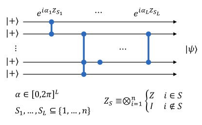
Figure 1: The structure of a commutative quantum circuit (CQC) in the Hadamard basis. Each circuit operation is a multiqubit $Z$-type rotation on a distinct subset of qubits. A maximal CQC on $n$ qubits consists of all $2^{n}-1$ $Z$-type rotations that act non-trivially on at least one qubit.

Consider a “maximal” circuit consisting of all $2^{n}$ $Z$-type rotations. Then $\alpha$ may be regarded as a vector over all length-$n$ bitstrings, where each bitstring specifies a particular subset of $\{1,\ldots,n\}$. A simple derivation shows that

$$|\psi\rangle =\frac{1}{\sqrt{2^{n}}}\sum_{x\in\{0,1\}^{n}}e^{\mathrm{i}\theta_{x}}|x\rangle$$ (6)

where $\theta\in\mathbb{R}^{2^{n}}$ is the Walsh-Hadamard transform of $\alpha$. It follows that the ability to prescribe all $2^{n}$ components of $\alpha$ implies the ability to prescribe all $d$ components of $\theta$. Since the circuit operation corresponding to $\alpha_{0}$ imparts an inconsequential global phase to the quantum state, that circuit operation may be omitted and the global phase may be chosen so that $\theta_{0}=0$. The output state may then be represented by a length-$2^{n}$ complex vector

$$\psi(\theta) =\left(\frac{1}{\sqrt{d}},\frac{e^{\mathrm{i}\theta_{1}}}{\sqrt{d}},\ldots,\frac{e^{\mathrm{i}\theta_{d-1}}}{\sqrt{d}}\right)$$ (7)

where $\theta_{1},\ldots,\theta_{d-1}$ can be independently varied. (Here $d=2^{n}$ and I have switched indices from bitstrings in $\{0,1\}^{n}$ to corresponding integers in $\{0,\ldots,2^{n}-1\}$.)

While maximal commutative quantum circuits are not practically realizable for large $n$ (the number of operations is $2^{n}-1$), they provide an upper bound on the expressiveness that can be achieved by any commutative quantum circuit with a given number of qubits. As I will now show, the expressiveness of a maximal commutative circuit, as measured by $\mathbb{E}\left[F^{t}\right]$, is proportional to $f_{2^{n}}(t)$. The fidelity $F$ is the square of the inner product

$$\psi(\theta)^{\dagger}\psi(\theta^{\prime}) =\frac{1}{d}\sum_{x=0}^{d-1}e^{\mathrm{i}(\theta_{x}^{\prime}-\theta_{x})}.$$ (8)

In terms of $\phi_{x}\equiv\theta_{x}^{\prime}-\theta_{x}$ we have

$$F(\psi(\theta),\psi(\theta^{\prime})) =\left|\psi(\theta)^{\dagger}\psi(\theta^{\prime})\right|^{2}=\frac{1}{d^{2}}\sum_{x,y=0}^{d-1}e^{\mathrm{i}(\phi_{x}-\phi_{y})},$$ (9)

$$F(\psi(\theta),\psi(\theta^{\prime}))^{t} =\frac{1}{d^{2t}}\sum_{x_{1},y_{1}=0}^{d-1}\cdots\sum_{x_{t},y_{t}=0}^{d-1}e^{\mathrm{i}(\phi_{x_{1}}+\cdots+\phi_{x_{t}})-\mathrm{i}(\phi_{y_{1}}+\cdots\phi_{y_{t}})},$$ (10)

and

$$\mathbb{E}\left[F(\psi(\theta),\psi(\theta^{\prime}))^{t}\right] =\frac{1}{d^{2t}}\sum_{x_{1},y_{1}=0}^{d-1}\cdots\sum_{x_{t},y_{t}=0}^{d-1}\mathbb{E}\left[e^{\mathrm{i}(\phi_{x_{1}}+\cdots+\phi_{x_{t}})-\mathrm{i}(\phi_{y_{1}}+\cdots\phi_{y_{t}})}\right].$$ (11)

Let us suppose the rotation angles $\alpha_{i}$ are drawn uniformly and independently from $[0,2\pi]$. Then each $\theta_{x}$ and $\theta_{x}^{\prime}$ are independent and uniform over $[0,2\pi]$, and $\phi_{x}$ is also uniform over $[0,2\pi]$. For each $i\in\{1,\ldots,d-1\}$, let $m_{i}(x)$ be the number of occurrences of $i$ in $(x_{1},\ldots,x_{t})$ and let $m_{i}(y)$ denote the number of occurrences of $i$ in $(y_{1},\ldots,y_{t})$. Then the summand may be written as

$$\mathbb{E}\left[e^{\mathrm{i}(\phi_{x_{1}}+\cdots+\phi_{x_{t}})-\mathrm{i}(\phi_{y_{1}}+\cdots\phi_{y_{t}})}\right] =\mathbb{E}\left[\prod_{i=1}^{d-1}e^{\mathrm{i}(m_{i}(x)-m_{i}(y))\phi_{i}}\right]$$ (12)

$$=\prod_{i=1}^{d-1}\mathbb{E}\left[e^{\mathrm{i}(m_{i}(x)-m_{i}(y))\phi_{i}}\right]$$ (13)

since the $\phi_{i}$’s are independent. Now,

$$\mathbb{E}\left[e^{\mathrm{i}(m_{i}(x)-m_{i}(y))\phi_{i}}\right] =\begin{cases}1&m_{i}(x)=m_{i}(y)\\ 0&m_{i}(x)\neq m_{i}(y)\end{cases}.$$ (14)

Thus the only pairs $(x,y)$ that contribute to $\mathbb{E}\left[F^{t}\right]$ are those for which $m_{i}(x)=m_{i}(y)$ for all $i=1,\ldots,d-1$. For such pairs it also holds that $m_{0}(x)=m_{0}(y)$. That is, a term contributes if and only if $x=(x_{1},\ldots,x_{t})$ is an anagram of $y=(y_{1},\ldots,y_{t})$, i.e. $xy$ is an abeliean square. It follows that

$$\mathbb{E}\left[F^{t}\right] =\frac{f_{d}(t)}{4^{nt}}.$$ (15)

Whereas $t$ is typically small, $d=2^{n}$ can be very large, which necessitates use of eq. (3).

It is convenient to compare $\mathbb{E}\left[F^{t}\right]$ for a given circuit to its minimal value

$$\mathbb{E}\left[F^{t}\right]_{\text{min}} =\binom{t+d-1}{t}^{-1}$$ (16)

which is achieved by a circuit that covers the entire state space uniformly. Fig. 2 plots the normalized expressiveness $\mathbb{E}\left[F^{t}\right]_{\text{min}}/\mathbb{E}\left[F^{t}\right]$. For all $d$, the normalized expressive is near 1 at small $t$ and decays to 0 at large $t$. This indicates that the circuits are highly expressive at coarse scales (small $t$), but have very low expressiveness at fine scales (large $t$). That is, the set of states that can achieved by maxmimal commutative quantum circuits span the breadth of the state space, but constitute only a sparse or low-dimensional subset of the state space.

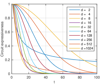
Figure 2: Normalized expressiveness $\mathbb{E}\left[F^{t}\right]_{\text{min}}/\mathbb{E}\left[F^{t}\right]$ of maximal commutative quantum circuits, as a function of the number of qubits $n$ and the resolving power $t$.

IV Acknowledgements

This work was performed at Oak Ridge National Laboratory, operated by UT-Battelle, LLC under contract DE-AC05-00OR22725 for the US Department of Energy (DOE). Support for the work came from the DOE Advanced Scientific Computing Research (ASCR) Accelerated Research in Quantum Computing Program under field work proposal ERKJ354.

References

- [1] Paul Erdős. Some unsolved problems. Michigan Math. J., 4(3):291–300, 1957.
- [2] Veikko Keränen. Abelian squares are avoidable on 4 letters. In W. Kuich, editor, Automata, Languages and Programming, Lecture Notes in Computer Science, pages 41–52, Berlin, Heidelberg, 1992. Springer.
- [3] Costas S. Iliopoulos, Dennis Moore, and W. F. Smyth. A characterization of the squares in a Fibonacci string. Theoretical Computer Science, 172(1):281–291, February 1997.
- [4] Arturo Carpi. On the number of Abelian square-free words on four letters. Discrete Applied Mathematics, 81(1):155–167, January 1998.
- [5] Julien Cassaigne, Gwénaël Richomme, Kalle Saari, and Luca Q. Zamboni. Avoiding abelian powers in binary words with bounded abelian complexity. Int. J. Found. Comput. Sci., 22(04):905–920, June 2011.
- [6] Mari Huova, Juhani Karhumäki, and Aleksi Saarela. Problems in between words and abelian words: K-abelian avoidability. Theoretical Computer Science, 454:172–177, October 2012.
- [7] M. Crochemore, C. S. Iliopoulos, T. Kociumaka, M. Kubica, J. Pachocki, J. Radoszewski, W. Rytter, W. Tyczyński, and T. Waleń. A note on efficient computation of all Abelian periods in a string. Information Processing Letters, 113(3):74–77, February 2013.
- [8] Ryan S. Bennink. Counting Abelian Squares More Efficiently. arXiv:2203.11886 [math.CO], March 2022.
- [9] L. B. Richmond and Jeffrey Shallit. Counting Abelian Squares. Electron. J. Combin., 16(1):R72, June 2009.
- [10] Jarrod R McClean, Jonathan Romero, Ryan Babbush, and Alán Aspuru-Guzik. The theory of variational hybrid quantum-classical algorithms. New J. Phys., 18(2):023023, February 2016.
- [11] Xiao Yuan, Suguru Endo, Qi Zhao, Ying Li, and Simon C. Benjamin. Theory of variational quantum simulation. Quantum, 3:191, October 2019.
- [12] Alicia B. Magann, Christian Arenz, Matthew D. Grace, Tak-San Ho, Robert L. Kosut, Jarrod R. McClean, Herschel A. Rabitz, and Mohan Sarovar. From Pulses to Circuits and Back Again: A Quantum Optimal Control Perspective on Variational Quantum Algorithms. PRX Quantum, 2(1):010101, January 2021.
- [13] Alberto Peruzzo, Jarrod McClean, Peter Shadbolt, Man-Hong Yung, Xiao-Qi Zhou, Peter J. Love, Alán Aspuru-Guzik, and Jeremy L. O’Brien. A variational eigenvalue solver on a photonic quantum processor. Nat Commun, 5(1):4213, September 2014.
- [14] Ying Li and Simon C. Benjamin. Efficient Variational Quantum Simulator Incorporating Active Error Minimization. Phys. Rev. X, 7(2):021050, June 2017.
- [15] Abhinav Kandala, Antonio Mezzacapo, Kristan Temme, Maika Takita, Markus Brink, Jerry M. Chow, and Jay M. Gambetta. Hardware-efficient variational quantum eigensolver for small molecules and quantum magnets. Nature, 549(7671):242–246, September 2017.
- [16] Guillaume Verdon, Jacob Marks, Sasha Nanda, Stefan Leichenauer, and Jack Hidary. Quantum Hamiltonian-Based Models and the Variational Quantum Thermalizer Algorithm. arXiv:1910.02071 [quant-ph], October 2019.
- [17] Sam McArdle, Tyson Jones, Suguru Endo, Ying Li, Simon C. Benjamin, and Xiao Yuan. Variational ansatz-based quantum simulation of imaginary time evolution. npj Quantum Information, 5(1):75–81, September 2019.
- [18] Jin-Guo Liu, Liang Mao, Pan Zhang, and Lei Wang. Solving quantum statistical mechanics with variational autoregressive networks and quantum circuits. Mach. Learn.: Sci. Technol., 2(2):025011, February 2021.
- [19] C. Kokail, C. Maier, R. van Bijnen, T. Brydges, M. K. Joshi, P. Jurcevic, C. A. Muschik, P. Silvi, R. Blatt, C. F. Roos, and P. Zoller. Self-verifying variational quantum simulation of lattice models. Nature, 569(7756):355–360, May 2019.
- [20] Harper R. Grimsley, Sophia E. Economou, Edwin Barnes, and Nicholas J. Mayhall. An adaptive variational algorithm for exact molecular simulations on a quantum computer. Nat Commun, 10(1):3007, December 2019.
- [21] Cristina Cîrstoiu, Zoë Holmes, Joseph Iosue, Lukasz Cincio, Patrick J. Coles, and Andrew Sornborger. Variational fast forwarding for quantum simulation beyond the coherence time. npj Quantum Inf, 6(1):1–10, September 2020.
- [22] Bryan T. Gard, Linghua Zhu, George S. Barron, Nicholas J. Mayhall, Sophia E. Economou, and Edwin Barnes. Efficient symmetry-preserving state preparation circuits for the variational quantum eigensolver algorithm. npj Quantum Inf, 6(1):10, December 2020.
- [23] Luogen Xu, Joseph T. Lee, and J. K. Freericks. Test of the unitary coupled-cluster variational quantum eigensolver for a simple strongly correlated condensed-matter system. Mod. Phys. Lett. B, 34(19n20):2040049, July 2020.
- [24] Anirban N. Chowdhury, Guang Hao Low, and Nathan Wiebe. A Variational Quantum Algorithm for Preparing Quantum Gibbs States. arXiv:2002.00055 [quant-ph], January 2020.
- [25] Edward Farhi, Jeffrey Goldstone, and Sam Gutmann. A Quantum Approximate Optimization Algorithm. arXiv:1411.4028 [quant-ph], November 2014.
- [26] Nikolaj Moll, Panagiotis Barkoutsos, Lev S. Bishop, Jerry M. Chow, Andrew Cross, Daniel J. Egger, Stefan Filipp, Andreas Fuhrer, Jay M. Gambetta, Marc Ganzhorn, Abhinav Kandala, Antonio Mezzacapo, Peter Müller, Walter Riess, Gian Salis, John Smolin, Ivano Tavernelli, and Kristan Temme. Quantum optimization using variational algorithms on near-term quantum devices. Quantum Sci. Technol., 3(3):030503, July 2018.
- [27] Vojtěch Havlíček, Antonio D. Córcoles, Kristan Temme, Aram W. Harrow, Abhinav Kandala, Jerry M. Chow, and Jay M. Gambetta. Supervised learning with quantum-enhanced feature spaces. Nature, 567(7747):209–212, March 2019.
- [28] Nathan Wiebe and Leonard Wossnig. Generative training of quantum Boltzmann machines with hidden units. arXiv:1905.09902 [quant-ph], May 2019.
- [29] Maria Schuld, Ryan Sweke, and Johannes Jakob Meyer. Effect of data encoding on the expressive power of variational quantum-machine-learning models. Phys. Rev. A, 103(3):032430, March 2021.
- [30] Jacob L. Beckey, M. Cerezo, Akira Sone, and Patrick J. Coles. Variational quantum algorithm for estimating the quantum Fisher information. Phys. Rev. Research, 4(1):013083, February 2022.
- [31] Andrey Kardashin, Alexey Uvarov, and Jacob Biamonte. Quantum Machine Learning Tensor Network States. Front. Phys., 8, 2021.
- [32] Xin Wang, Zhixin Song, and Youle Wang. Variational Quantum Singular Value Decomposition. Quantum, 5:483, June 2021.
- [33] Michael Lubasch, Jaewoo Joo, Pierre Moinier, Martin Kiffner, and Dieter Jaksch. Variational quantum algorithms for nonlinear problems. Phys. Rev. A, 101(1):010301, January 2020.
- [34] Zoë Holmes, Kunal Sharma, M. Cerezo, and Patrick J. Coles. Connecting Ansatz Expressibility to Gradient Magnitudes and Barren Plateaus. PRX Quantum, 3(1):010313, January 2022.
- [35] Sukin Sim, Peter D. Johnson, and Alán Aspuru-Guzik. Expressibility and Entangling Capability of Parameterized Quantum Circuits for Hybrid Quantum-Classical Algorithms. Advanced Quantum Technologies, 2(12):1900070, 2019.
- [36] Stig Elkjær Rasmussen, Niels Jakob Søe Loft, Thomas Bækkegaard, Michael Kues, and Nikolaj Thomas Zinner. Reducing the Amount of Single-Qubit Rotations in VQE and Related Algorithms. Advanced Quantum Technologies, 3(12):2000063, 2020.
- [37] Dan Shepherd and Michael J. Bremner. Instantaneous Quantum Computation. Proc. R. Soc. A, 465(2105):1413–1439, May 2009.
- [38] Michael J. Bremner, Richard Jozsa, and Dan J. Shepherd. Classical simulation of commuting quantum computations implies collapse of the polynomial hierarchy. Proc. R. Soc. A, 467(2126):459–472, February 2011.
- [39] Brian Coyle, Daniel Mills, Vincent Danos, and Elham Kashefi. The Born supremacy: Quantum advantage and training of an Ising Born machine. npj Quantum Inf, 6(1):1–11, July 2020.