Precedence-Constrained Arborescences

Abstract

The minimum-cost arborescence problem is a well-studied problem in the area of graph theory, with known polynomial-time algorithms for solving it. Previous literature introduced new variations on the original problem with different objective function and/or constraints. Recently, the Precedence-Constrained Minimum-Cost Arborescence problem was proposed, in which precedence constraints are enforced on pairs of vertices. These constraints prevent the formation of directed paths that violate precedence relationships along the tree. We show that this problem is NP-hard, and we introduce a new scalable mixed integer linear programming model for it. With respect to the previous models, the newly proposed model performs substantially better. This work also introduces a new variation on the minimum-cost arborescence problem with precedence constraints. We show that this new variation is also NP-hard, and we propose several mixed integer linear programming models for formulating the problem.

1 Introduction

The Minimum-Cost Arborescence problem (MCA) is a well-known problem that consists in finding a directed minimum-cost spanning tree rooted at some vertex $r$ called the root in a directed graph. The first polynomial time algorithm for solving the problem was proposed independently by Yoeng-Jin Chu and Tseng-Hong Liu [8], and Jack Edmonds [11]. The problem can be formally described as follows. A directed graph $G=(V,A)$ is given where $V=\{1,\cdots,n\}$ is the set of vertices, $r\in V$ is the root of the arborescence, and $A\subseteq V\times V$ is the set of arcs with a cost $c_{a}$ associated with every arc $a\in A$. The goal is to find a minimum-cost directed spanning tree in $G$ rooted at $r$, i.e. a set $T\subseteq A$ of $n-1$ arcs, such that there is a unique directed path from $r$ to any other vertex $j\in V\setminus\{r\}$ in the subgraph induced by $T$. A different polynomial time algorithm for solving the MCA that operates directly on the cost matrix was discussed by Bock [4].

Since the MCA was first proposed, different variations have been introduced such as the Resource-Constrained Minimum-Weight Arborescence problem [15], where finite resources are associated with each vertex in the input graph. The objective of the problem is to find an arborescence with minimum total cost where the sum of the costs of outgoing arcs from each vertex is at most equal to the resource of that vertex. The problem is categorized as NP-hard as it generalizes the Knapsack problem [15]. The Capacitated Minimum Spanning Tree problem [19] is another variation, where non-negative integer node demands $q_{j}$ is associated with each node $j\in V\backslash\{r\}$, and an integer $Q$ is given. The objective is to find a minimum spanning tree rooted at $r$ such that the sum of the weights of the vertices in any subtree off the root is at most $Q$. The problem is shown to be NP-hard as the particular case with zero cost arcs is a bin packing problem [19]. The $p$-Arborescence Star problem [30] is a relevant problem that is described as follows. Given a weighted directed graph $G=(V,A)$, a root vertex $r\in V$, and an integer $p$, the objective of the problem is to find a minimum-cost reverse arborescence rooted at $r$, such that the arborescence spans the set of vertices $H\subseteq V\backslash\{r\}$ of size $p$, and each vertex $v\in V\backslash\{H\cup r\}$ must be assigned to one of the vertices in $H$. The problem is NP-hard [29] in the general case by a reduction from the $p$-median problem [20]. Frieze and Tkocz [16] study the problem of finding a minimum-cost arborescence such that the cost of the arborescence is at most $c_{0}$. The problem is studied on randomly weighted digraphs where each arc in the graph has a weight $w$ and a cost $c$, each being an independent uniform random variable $U^{s}$ where $0<s\leq 1$, and $U$ is uniform $[0,1]$. The problem is NP-hard [16] through a reduction from the knapsack problem. Another problem is the Maximum Colorful Arborescence problem [14] which can be described as the following. Given a weighted directed acyclic graph with each vertex having a specified color from a set of colors $C$, the objective is to find an arborescence of maximum weight, in which no color appears more than once. The problem is known to be NP-hard [5] even when all arcs have a weight of 1. The Constrained Arborescence Augmentation problem [25] is a different variation that can be described as follows. Given a weighted directed graph $G=(V,A)$, and an arborescence $T=(V,A_{r})$ in $G$ rooted at vertex $r\in V$, the objective of the problem is to find an arc subset $A^{\prime}$ from $A-A_{r}$ such that there still exists an arborescence in the new graph $G^{\prime}=(V,A_{r}\cup A^{\prime}-{a})$ for each arc $a\in A_{r}$, where the sum of the weights of the arcs in $A^{\prime}$ is minimized. The problem is an extension on the augmentation problem [13], and is shown to be NP-hard [25]. The Minimum $k$ Arborescence with Bandwidth Constraints [6] is another variation, where every arc $a\in A$ has an integer bandwidth $b(a)$ that indicates the number of times such an arc can be used. The objective of the problem is to find $k$ arborescences of minimum-cost rooted at the $k$ given root vertices, covering every arc $a\in A$ at most $b(a)$ times. It has been shown that the problem can be solved in polynomial time [6]. The Degree-Constrained Minimal Spanning Tree problem with unreliable links and node outage costs [23] is modeled as a directed graph with the root vertex being the central node of a network, and all other vertices being terminal nodes. The problem consists in finding links in a network to connect a set of terminal nodes to a central node, while minimizing both link costs and node outage costs. Node outage cost is the economic cost incurred by the network user whenever that node is disabled due to failure of a link. The problem is shown to be NP-hard by reducing the problem to an equivalent Traveling Salesman problem [18]. The Minimum Changeover Cost Arborescence [17] is another variation, where each arc is labeled with a color out of a set of $k$ available colors. A changeover cost is defined on every vertex $v$ in the arborescence other than the root. The cost over a vertex $v$ is paid for each outgoing arc from $v$ and depends on the color of its outgoing arcs, relative to the color of its incoming arc. The costs are given through a $k\times k$ matrix $C$, where each entry $C_{ab}$ specifies the cost to be paid at vertex $v$ when its incoming arc is colored $a$ and one of its outgoing arcs is colored $b$. A change over cost at vertex $v$ is calculated as the sum of costs paid for every outgoing arc at that vertex. The objective of the problem is to find an arborescence $T$ with minimum total change over cost for every vertex $j\in V$ other than the root. The problem is shown to be NP-hard and very hard to approximate [17]. Finding a pair of arc-disjoint in-arborescence and out-arborescence is another problem, with the objective of finding a pair of arc-disjoint $r$-out-arborescence rooted at $r_{1}$ and $r$-in-arborescence rooted at $r_{2}$ where $r_{1},r_{2}\in V$. An $r$-out-arborescence has all its arcs directed away from the root, and an $r$-in-arborescence has all its arcs directed towards the root. The problem was studied by Bérczi et al. [3] where a linear-time algorithm for solving the problem in directed acyclic graphs is proposed. The problem is shown to be NP-Complete in general graphs even if $r_{1}=r_{2}$ [2]. Yingshu et al. [26] studied the problem of constructing a strongly connected broadcast arborescence with bounded transmission delay, where they devise a polynomial time algorithm for constructing a broadcast network with minimum energy consumption that respects the transmission delays of the broadcast tree simultaneously. The Minimum Spanning Tree Problem with Conflict Pairs is a variation of the minimum spanning tree problem where given an undirected graph and a set $S$ that contains conflicting pairs of edges called a conflict pair, the objective of the problem is to find a minimum-cost spanning tree that contains at most one edge from each conflict pair in $S$ [7]. The problem is shown to be NP-hard [9]. The Least-Dependency Constrained Spanning Tree problem [34] is another variation that can be defined as follows. Given a connected graph $G=(V,E)$ and a directed graph $D=(E,A)$ whose vertices are the edges of $G$, the directed graph $D$ is a dependency graph for $E$, and $e_{1}\in E$ is a dependency of $e_{2}\in E$ if $(e_{1},e_{2})\in A$. The objective of the problem is to decide whether there is a spanning tree $T$ of $G$ such that each edge in $T$ has either an empty dependency or at least one of its dependencies is also in $T$. The All-Dependency Constrained Spanning Tree problem [34] is a similar problem that consists in deciding whether there is a spanning tree $T$ of $G$ such that each of its edges either has no dependency or all of its dependencies are in $T$. The two problems are shown to be NP-Complete [34].

The Precedence-Constrained Minimum-Cost Arborescence problem (PCMCA) was first introduced by Dell’Amico et al. [10], where a set of precedence constraints is included as follows. Given a set $R$ of ordered pairs of vertices, then for each precedence $(s,t)\in R$ any path of the arborescence covering both vertices $s$ and $t$ must visit $s$ before visiting $t$. The objective of the problem is to find an arborescence of minimum total cost that satisfies the precedence constraints. By definition of the PCMCA, we always assume that if $(s,t)\in R$ then $(t,s)\notin A$. The PCMCA has applications in infrastructure design such as designing a commodity distribution network. As an example, assume we have a commodity distribution network, where the distribution starts from a main vertex (root of the arborescence), and the distribution travels in a single direction away from the root to every other vertex in the graph. Such a structure follows the definition of an arborescence. Now assume that transit duties that are higher than the travel costs have to be paid by vertex $s$ in the graph, if the commodity passes through vertex $t$ on its way to vertex $s$. To avoid for such duties to be paid by vertex $s$, we can impose a precedence relationship between the vertex pair $s$ and $t$, i.e. $(s,t)\in R$. This will guarantee that no directed path from $t$ to $s$ will appear in the distribution network, and vertex $s$ can avoid paying the transit duties (see [10] for more details).

A new variation on the MCA named the Precedence-Constrained Minimum-Cost Arborescence problem with Waiting Times (PCMCA-WT) is introduced in this work. The problem is an extension on the PCMCA characterized by an additional constraint. Given a spanning arborescence rooted at vertex $r$, with arc costs indicating the time required to traverse an arc, assume there is a flow which starts at the root vertex $r$ and traverses each path of the arborescence. For each precedence $(s,t)\in R$, we must guarantee that the time at which the flow enters $s$ is smaller than or equal to the time at which the flow enters $t$. As an example, assume that $(b,a),(c,a),(d,a)\in R$, and the flow enters vertex $b$ at time step 5, vertex $c$ at time step 10, and vertex $d$ at time step 15. Therefore, the flow must enter vertex $a$ at a time step greater than or equal to 15, and if the cost of the path from $r$ to $a$ is equal to 10, then this will result in a waiting time of 5 at vertex $a$. The objective of the problem is to find an arborescence $T$ that has a minimum total cost, plus total waiting times, where the flow never enters $t$ earlier than entering $s$ for all $(s,t)\in R$.

The contributions of this paper can be summarized as:

1. Introducing a scalable and efficient integer linear programming model for the PCMCA.

2. Introducing the PCMCA-WT as a new variation of the MCA.

3. Proving that both the PCMCA and the PCMCA-WT are NP-hard.

The rest of the paper is organized as follows. Section 2 presents a proof of complexity and a new mixed integer linear programming model (MILP) for the PCMCA. Section 3 presents a proof of complexity and several mixed integer linear programming models for the PCMCA-WT. Section 4 discusses computational results, while some conclusions are summarized in Section 5.

2 The Precedence-Constrained Minimum-Cost Arborescence Problem

The Precedence-Constrained Minimum-Cost Arborescence problem can be formally described as follows. Let $G=(V,A)$ be a directed graph, $r\in V$, and $P=(V,R)$ be a precedence graph. Let $c_{ij}$ be a cost associated with every arc $(i,j)\in A$. An arc $(s,t)\in R$ is a precedence relationship between the two vertices $s,t\in V$. The objective of the problem is to find a minimum-cost arborescence $T$ rooted at vertex $r\in V$ such that, for each $(s,t)\in R$, $t$ must not belong to the unique path in $T$ that connects $r$ to $s$. For simplicity, we always assume that for the root $r\in V$, $(s,r)\notin A$ for all $s\in V\backslash\{r\}$, as by definition none of these arcs would be part of an arborescence rooted at $r$, and $(s,r)\notin R$ for all $s\in V\backslash\{r\}$ as the problem would be infeasible otherwise.

Figure 1 presents an example that shows the difference between the classic MCA and the PCMCA. The example instance graph with its respective arc costs is shown in the figure on the left, with the precedence relationship $(3,1)$ highlighted in red. The figure in the middle shows a feasible MCA solution with a cost of 3. The MCA solution is infeasible for the PCMCA since $(3,1)\in R$, and vertex 1 belongs to the directed path connecting $r$ to vertex 3. To make the solution feasible for the PCMCA, vertex 1 must succeed vertex 3 on the same directed path, or the two vertices must reside on two disjoint paths. A feasible solution with a cost of 4 is shown in the figure on the right.

Figure 1: Comparing a MCA and a PCMCA solution. The graph on the left shows the instance graph with its respective arc costs, with the precedence relationship $(3,1)\in R$ highlighted in red. The graph in the middle shows the optimal MCA, and the graph on the right shows the optimal PCMCA. The MCA solution is not a feasible PCMCA solution since vertex 1 precedes vertex 3 on the same directed path and $(3,1)\in R$.

2.1 Computational Complexity

Some of the Minimum-Cost Arborescence variations mentioned in Section 1 belong to the NP-hard complexity class. In this section we show that the Precedence-Constrained Minimum-Cost Arborescence Problem is also NP-hard. The proof is inspired by the one introduced in [24] for the Path Avoiding Forbidden Pairs problem.

Theorem 1.

The PCMCA is NP-hard.

Figure 2: A PCMCA instance reduced from 3-SAT. The set of vertices $v_{ij}\subset V$ are the literals of the 3-SAT problem, where each layer is a clause that is completely connected only to the clause in the next layer. Dashed arcs show the precedence constraints $R$ between pairs of vertices. As an example, we assume literal $v_{11}$ is the negation of $v_{m1}$, therefore there is a precedence relationship $(v_{m1},v_{11})\in R$ which will enforce that no literal and its negation can belong to the same path.

Proof.

By reduction from 3-SAT: Let $X=\{x_{1},x_{2},\dots,x_{t}\}$ be a set of variables. Let $\Phi=C_{1}\,\wedge\,C_{2}\,\wedge\,\dots\wedge\,C_{m}$ be a boolean expression in 3-conjunctive normal form, such that each clause $C_{i}$, $i=1,\dots,m$, is denoted by $(v_{i1}\vee v_{i2}\vee v_{i3})$, where each literal $v_{ik},1\leq k\leq 3$, is associated to one variable in $X$ or its negation. We will construct a graph $G$ and a set of precedence constraints $R$ such that there exists a feasible solution of the PCMCA problem in $G$ if and only if $\Phi$ is satisfiable.

Let $G=(V,A)$ where $V=\{r\}\cup\{s\}\cup\{s^{\prime}\}\cup\{t\}\cup C$, with $C$, $A$ and $R$ defined as follows.

$$C ={\{v_{ik}:1\leq i\leq m,1\leq k\leq 3\}}$$

$$A =\{(r,s),(r,s^{\prime})\}\cup\{(s,v_{1j}),1\leq j\leq 3)\}\cup\{(v_{mj},t),1\leq j\leq 3\}$$

$$\cup\{(v_{ij},v_{i+1,k}),1\leq i<m,1\leq j,k\leq 3\}\cup\{(s^{\prime},v_{ij}),1\leq i\leq m,1\leq j\leq 3\}$$

$$R =\{(t,s^{\prime})\}\cup\{(v_{hk},v_{ij}):h>i,\,v_{hk}\text{ and }v_{ij}\text{ refer to the same variable, but}$$

$$\quad\,\,\,\text{exactly one of the two literals is negated}\}$$

Note that $C$ contains $3m$ vertices, one for each literal of each clause $C_{i}$, with all arcs having an equal positive cost. The three sets $C$, $A$, and $R$ induce the graph shown in Figure 2. The set of precedence constraints, besides $(t,s^{\prime})$, is between two vertices that refer to the same literal, but exactly one of the two literals is negated. If a feasible solution $T$ of the PCMCA problem can be found in $G$, this implies that:

1. no path from $s^{\prime}$ to $t$ exists in $T$

2. in any (rooted) path there is no pair of vertices corresponding to a variable and its negation

3. there is a unique path $P$ from $r$ to $t$ which passes through $s$ and through a vertex of each clause

The formula can be satisfied by assigning true values to all the literals corresponding to the vertices in $P\cap C$, and assigning false values to all the variables not associated with these literals. This satisfies all the clauses.

Conversely, if the formula is satisfied then each clause has at least one literal with true value, and no variable is assigned to both true and false (in different clauses). We construct a PCMCA feasible solution as follows. We start by building a path $P$ from $r$ to $t$ which includes $s$ and exactly one vertex from each clause, corresponding to a literal with true value. We complete the arborescence by adding $(r,s^{\prime})$ and $(s^{\prime},v)$ for each $v\not\in P$. ∎

2.2 A Set-Based Model

The MILP previously proposed in [10] suffers from scalability issues because of the cubic number of variables (relative to the number of vertices and the precedence relationships) used to model the precedence relationships between vertex pairs. A new integer linear program for the PCMCA is introduced in this section.

We extend the classic connectivity constraints for the MCA [22] in such a way to take precedences into account. When considering a set $S\subseteq V\backslash\{r\}$ we add a constraint for each $j\in S$, and we force that at least one active arc must enter $S$ coming from the set of vertices allowed to precede $j$ on the path connecting $j$ to $r$.

Let $x_{ij}$ be a variable associated with every arc $(i,j)\in A$ such that $x_{ij}=1$ if $(i,j)\in T$ and 0 otherwise, where $T$ is the resulting optimal arborescence. Let $V_{j}=\{i\in V:(j,i)\notin R\}$ be the set of vertices that can precede $j$ on a directed path from the root without introducing precedence violations or, in turn, a violating path, which is a directed path that violates some precedence relationship in $R$.

minimize $$\sum_{(i,j)\in A}c_{ij}x_{ij}$$ (1)

subject to $$\sum_{(i,j)\in A}x_{ij}=1 \forall j\in V\backslash\{r\}$$ (2)

$$\sum_{\begin{subarray}{c}(i,k)\in A:\\ i\in V_{j}\backslash S,\,k\in S\end{subarray}}x_{ik}\geq 1 \forall j\in V\backslash\{r\},\forall S\subseteq V_{j}\backslash\{r\}:j\in S$$ (3)

$$x_{ij}\in\{0,1\} \forall(i,j)\in A$$ (4)

Constraints (2) implies the first property of an arborescence namely that every vertex $v\in V\backslash\{r\}$ must have a single parent. Constraints (3) model the connectivity constraints, that is every vertex $j\in V\backslash\{r\}$ must be reachable from the root. Note that $V_{j}\backslash S$ contains at least $r$, while $S$ contains at least $j$. The set of constraints (3) reduces to the classical connectivity constraints for the MCA which are $\sum_{(i,k)\in A:\,i\notin S,\,k\in S}x_{ik}\geq 1$ $\forall S\subseteq V\backslash\{r\}$ when the set $R$ of precedence relationships is empty. This is because when $R$ is an empty set, $V_{j}=V$ for all $j\in V\backslash\{r\}$. Constraints (3) also impose the precedence relationships. Inequality (3) implies that the resulting arborescence will not include vertex $t$ in the directed path connecting $r$ to $s$ when $(s,t)\in R$. Note that this is the same inequality named weak $\sigma$-inequality considered by Ascheuer, Jünger & Reinelt [1] for the Sequential Ordering Problem. Finally, constraints (4) define the domain of the variables. The MILP model proposed has $O(|A|)$ variables, and $O(|A|)$ constraints, plus an exponential number of connectivity constraint (3). Although the number of constraints of the Set-Based Model is exponential, it is more efficient at solving the problem than the model introduced in [10]. This is because in practice the number of constraints that are dynamically added to the model is small. Moreover, the model uses a smaller number of variables. An experimental validation for these considerations will be provided by the experiments in Section 4.

One approach to solve a linear relaxation model (LR-model) that has an exponential number of constraints is to start by solving the LR-model without including a large set of constraints (such as (3)), then iteratively adding a constraint once it is violated, then solving the new LR-model again. A procedure for finding a violated constraint is called a separation procedure. The optimal solution of the LR-model is found as soon as there are no violated constraints. When solving a MILP, the optimality gap needs to be closed to find the optimal solution even if no violated inequality is found.

In the literature, the large set of constraints that are necessary to model the problem, but are added dynamically to the model only when they are violated, are known as lazy constraints. Note that using this approach, the separation procedure must also be used to check the feasibility of integer solutions found by the linear relaxation or primal heuristics.

1:$G=(V,A)$ is a directed graph, $\bar{x}$ is a fractional LP-solution

2:procedure Find_Violated_Inequality($G$, $\bar{x}$)

3:     for $j\in V\backslash\{r\}$ do

4:         Construct a directed graph ${D_{j}}=(V_{j},A^{\prime})$ such that:

5:         $V_{j}=\{i\in V:(j,i)\notin R\}$

6:         $A^{\prime}=\{(i,k)\in A\,|\,i,k\in V_{j}\}$

7:         $c_{ik}=\bar{x}_{ik}\,\,\,\,\forall\,(i,k)\in A^{\prime}$

8:         Calculate a minimum $(r,j)$-cut $C$ in ${D_{j}}$

9:         if $\text{the cost of }C<1$ then

10:              return the violated inequality $\sum_{(i,k)\in C\,\,}x_{ik}\geq 1$

11:         end if

12:     end for

13:end procedure

Algorithm 1 Separation Procedure for Inequalities (3)

Algorithm 1 describes the separation procedure for inequalities (3). Let $\bar{x}$ be a solution of the linear relaxation or a candidate primal solution. An inequality (3) that is violated by the solution $\bar{x}$ can be detected by computing a minimum $(r,j)$-cut $C$ in a directed graph $D_{j}=(V_{j},A^{\prime})$, where $A^{\prime}$ is equal to the set of arcs $A$ minus the arcs incident to the immediate successors of $j$ in the precedence graph. The cost $c_{ik}$ of an arc $(i,k)\in A^{\prime}$ is equal to $\bar{x}_{ik}$. The value of the minimum $(r,j)$-cut $C$ in $D_{j}$ can tell us the following about the given fractional solution:

1. If the cost of a minimum cut is equal to 0, then vertex $j$ is not reachable from $r$ in $D_{j}$. In this case, the solution does not contain a path from $r$ to $j$, or contains a single or multiple paths from $r$ to $j$, all of which pass through a successor of $j$.

2. If the cost of a minimum cut is in the range $(0,1)$, then vertex $j$ is reachable from $r$ in $D_{j}$. In this case, the solution contains multiple paths from $r$ to $j$, and at least one of them passes through a successor of $j$.

3. If the cost of a minimum cut is equal to 1, then vertex $j$ is reachable from $r$ through a single or multiple paths in $D_{j}$, although possibly some of them pass through a successor of $j$.

In the first two cases, the minimum cut $C$ defines an inequality (3) violated by $\bar{x}$, however in the last case a violated inequality (3) does not exist even if the fractional solution $\bar{x}$ contains a violating path. Therefore, although inequalities (3) are valid inequalities for that PCMCA, there are fractional LP-solutions that contain violating paths, but satisfy inequalities (3).

Figure 3 shows an example on how the separation procedure works. The figure also shows a fractional solution of the Set-Based model that contains a violating path, but does not violate any inequality (3). Another example, showing how the Path-Based model introduced in [10] fails to detect a violating path in a fractional solution, is presented in A.

A drawback of the Set-Based model is the high computational complexity of the separation procedure of inequalities (3), which has a complexity of $O(n^{4})$, assuming it uses an $O(n^{3})$ algorithm for computing a minimum $(s,t)$-cut in $D_{j}$ [21].

Figure 3: An example of a fractional solution of the Set-Based model that contains a violating path, and does not violate an inequality (3). Every arc cost is associated with the value of its respective variable $x_{ij}$. For this solution we have the violated precedence $(s,t)\in R$. The figure on the left shows the solution, and the figure on the right shows the graph ${D_{j}}$ which has a minimum $(r,s)$-cut of value 1 indicated by the red dashed line.

3 The Precedence-Constrained Minimum-Cost Arborescence Problem with Waiting Times

Figure 4: Comparing an instance solved as a PCMCA, and solved as a PCMCA-WT. The graph on the left shows the instance with its respective arc costs, and the precedence relationship $(2,3)\in R$ highlighted in red. The graph in the middle shows the optimal PCMCA solution of cost 3, and the graph on the right shows the optimal PCMCA-WT solution of cost 4. The PCMCA solution is not a feasible PCMCA-WT solution since the flow enters vertex 3 before entering vertex 2 and $(2,3)\in R$.

In the Precedence-Constrained Minimum-Cost Arborescence Problem with Waiting Times (PCMCA-WT) a flow starts from the root $r$ at time 0, and traverses each path of the arborescence. The cost $c_{ij}$ of an arc $(i,j)\in A$ represents the time required to traverse that arc. Let $d_{j}$ be the time at which the flow enters vertex $j\in V$. For any $(s,t)\in R$, $d_{t}\geq d_{s}$, which means that the flow must enter vertex $t$ at the same time step or after entering vertex $s$. Let $w_{j}$ be the waiting time before the flow enters vertex $j$ required to respect the aforementioned constraint. The objective is to find an arborescence $T$ that has a minimum total cost plus total waiting time, where the flow never enters $t$ earlier than entering $s$ for all $(s,t)\in R$. For simplicity, we always assume that for the root $r\in V$, $(i,r)\notin A$ for all $i\in V\backslash\{r\}$, as by definition none of these arcs would be part of an arborescence rooted at $r$, and $(s,r)\notin R$ for all $s\in V\backslash\{r\}$, as the problem would be infeasible otherwise.

Figure 4 presents an example that shows the difference between the PCMCA and the PCMCA-WT. Next to each vertex we have its corresponding $d_{t}$ value. In this example we have the precedence relationship $(2,3)$ highlighted in red. The two solutions depicted are valid solutions for the PCMCA, since they both satisfy the precedence constraints, that is $t$ never precede $s$ on the same directed path for all $(s,t)\in R$. The solution in the middle shows the optimal PCMCA solution with a total cost of 3 (sum of all the arcs). We can see that the solution in the middle is not a feasible PCMCA-WT solution since $(2,3)\in R$ but $d_{3}<d_{2}$. The solution on the right shows an optimal PCMCA-WT solution with a cost of 4 (sum of all the arcs plus waiting time at each vertex). The solution results in a waiting time of 1 at vertex 3, since the time from $r$ to $2$ is 2, and the time from $r$ to $3$ is 1.

3.1 Computational Complexity

In this section we show that the PCMCA-WT is NP-hard.

The Rectilinear Steiner Arborescence (RSA) Problem [32] is an NP-hard problem formally defined as follows. Let $P=\{p_{1},p_{2},\dots,p_{n}\}$ be a set of points in the first quadrant of the Cartesian plane, where $p_{i}=(x_{i},y_{i})$ with $x_{i},y_{i}\geq 0$, and $p_{1}=(0,0)$. A complete grid can be created, where the points in P are on the intersections of vertical and horizontal lines. A set $S$ of Steiner vertices can be added, corresponding to the $O(|P|^{2})$ intersection points not overlapping with the points in $P$. The arcs of the problem are the right-directed horizontal segments and the up-directed vertical segments between two adjacent points of the grid $P\cup S$. The cost associated with each arc $(p_{i},p_{j})$ is defined as $|x_{i}-x_{j}|+|y_{i}-y_{j}|$. Figure 5 shows an example of an RSA instance with 5 points, and the relative Steiner vertices.

Given a positive value $k$, the decision version of the RSA problem consists in deciding whether there is an arborescence with total length not greater than $k$ such that the arborescence is rooted at $p_{1}$ and it contains a unique path from $p_{1}$ to $p_{i}$ for all $i\in\{1,2,\dots,{n}\}$. Note that the length of each path from $p_{1}$ to $p_{i}$ is $x_{i}+y_{i}$ by construction.

Figure 5: The figure shows an RSA instance with 5 points and 10 Steiner vertices, while the dashed lines represent the arcs of the instance.

Theorem 2.

The PCMCA-WT is NP-hard.

Proof.

By a reduction from the decision version of the RSA problem: we construct a graph $G=(V,A)$ and a set $R$ of precedence constraints such that there exist a PCMCA-WT solution of cost at most $k$ if and only if a RSA of cost at most $k$ exists. Given an instance of the RSA problem with a set of points P and a set of Steiner points S, consider the PCMCA-WT instance defined as follows:

$${V}\mkern 150.0mu \mkern-100.0mu{=\,P\cup S}$$

$${A^{\prime}}\mkern 150.0mu \mkern-100.0mu{=\{(i,j):\text{$j$ is immediately on the top of $i$ in the grid, or $j$ is im-}}$$

  mediately on the right of $$i$$ in the grid}

$${A}\mkern 155.0mu \mkern-100.0mu{=\,A^{\prime}\cup\{(P_{FAR},s_{i}),s_{i}\in S\}\text{, with }{P_{FAR}\in\operatorname*{argmax}_{p_{i}\in P}\{x_{i}+y_{i}\}}\mkern 100.0mu}$$

$${R}\mkern 155.0mu \mkern-100.0mu{=\,\{(p,P_{FAR}):p\in P\setminus\{P_{FAR}\}\}}$$

$${c_{ij}}\mkern 150.0mu \mkern-100.0mu{=\,(x_{j}-x_{i})+(y_{j}-y_{i})\text{ for }(i,j)\in A^{\prime}}$$

$${c_{P_{FAR},s_{i}}}\mkern 110.0mu \mkern-100.0mu{=\,0\text{ for }s_{i}\in S}$$

Figure 6: The PCMCA-WT instance associated with the RSA instance depicted in Figure 5. A RSA solution of minimum cost is given by the blue arcs. The red arcs have cost 0 and, together with the blue ones, form an optimal PCMCA-WT solution.

If the instance of RSA has a solution of cost $k$, then a solution of cost $k$ for the instance of PCMCA-WT can be obtained. Starting from the solution of the RSA problem, it is possible to complete the solution of the associated PCMCA-WT problem by adding 0-cost arcs (red arcs) to connect the node $P_{FAR}$ to the Steiner nodes not used in the RSA solution. The solution of an RSA instance and a solution of the associated PCMCA-WT problem are depicted in Figure 6.

Conversely, assume that there is a feasible solution of PCMCA-WT with cost at most $k$. Without loss of generality suppose that such a solution is optimal. Note that a path starting at $P_{FAR}$ and passing through a vertex in $P$ cannot exist due to the precedence constraints. Besides, every leaf of the arborescence that is in $S$ must have $P_{FAR}$ as parent; otherwise, making $P_{FAR}$ its parent would reduce the cost. Therefore, removing all the leaves of the PCMCA-WT arborescence connected through $P_{FAR}$ results in a tree that uses only arcs in $A^{\prime}$ and whose leaves are all in $P$. It follows that the resulting tree is a feasible solution for the RSA.

∎

3.2 MILP Models

This section introduces three different MILP models for formulating the Precedence-Constrained Minimum-Cost Arborescence Problem with Waiting Times. For all the models, let $d_{j}$ be a variable associated with every vertex $j\in V$ to represent the time at which the flow enters vertex $j$, with $d_{r}=0$. The value of $d_{j}$ is bounded from below by summing the time from $r$ to the parent $i$ of $j$ and the cost of the arc $(i,j)\in A$ that is part of the arborescence. To ensure that the resulting arborescence satisfies the precedence constraints, we enforce that the time from $r$ to $t$ is greater than or equal to the time from $r$ to $s$ for all $(s,t)\in R$. A variable $x_{ij}$ is associated with every arc $(i,j)\in A$ such that $x_{ij}=1$ if $(i,j)\in T$ and 0 otherwise, where $T$ is the resulting optimal arborescence.

In all the models proposed for the PCMCA-WT, the value of $M$, which is an upper bound on the value of an optimal solution, is equal to the solution cost of solving the instance as a Sequential Ordering Problem (SOP) [28] using a nearest neighbor algorithm [33]. This is a valid upper bound on the solution for the PCMCA-WT, since a valid solution for the SOP consists of a simple directed path that includes all the vertices of the graph such that $t$ never precede $s$ for all $(s,t)\in R$, which implies that $d_{t}\geq d_{s}$ for all $(s,t)\in R$, and the waiting time on each vertex is equal to zero.

3.2.1 A Multi-Commodity Flow Model

The model introduced in this section extends the one introduced in [10] for the PCMCA, and formulates the sub-problem of finding an arborescence rooted at $r$ that does not violate precedence relationships in $R$ as a multi-commodity flow problem. The model uses a polynomial set of constraints instead of inequalities (3) to ensure that every vertex in the graph is reachable from the root, and that for any $(s,t)\in R$ there is no path from $r$ to $s$ that passes through $t$ in the resulting arborescence. This can be ensured by having a flow value of 1 that enters every vertex $k$ in the graph, and that for any vertex $k$ the flow to that vertex does not pass through a successor of $k$. Let $y^{k}_{ij}$ be a variable associated with every vertex $k\in V\backslash\{r\}$ and every arc $(i,j)\in A$, such that $y^{k}_{ij}=1$ if arc $(i,j)\in A$ is part of the path from the root $r$ to vertex $k$, and 0 otherwise. Let $w_{i}$ be the waiting time at vertex $i\in V$.

(MCF)minimize $$\mkern-100.0mu\sum_{\begin{subarray}{c}(i,j)\in A\end{subarray}}c_{ij}x_{ij}+\sum_{i\in V}w_{i}$$ (5)

subject to $$\mkern-150.0mu\sum_{(i,j)\in A}x_{ij}=1\mkern 260.0mu\forall j\in V\backslash\{r\}$$ (6)

$$\mkern-150.0mu\sum_{\begin{subarray}{c}(i,j)\in A:\\ (k,j)\notin R\end{subarray}}y^{k}_{ij}-\sum_{\begin{subarray}{c}(j,i)\in A:\\ (k,j)\notin R\end{subarray}}y^{k}_{ji}=\left\{\begin{array}[]{l}1\mbox{ if }i=r\\ \mkern-14.0mu-1\mbox{ if }i=k\\ 0\mbox{ otherwise}\end{array}\right.\mkern-15.0mu\begin{array}[]{r}\forall k\in V\backslash\{r\},\\ \forall i\in V:(k,i)\notin R\end{array}$$ (12)

$$\mkern-150.0mud_{r}=0$$ (13)

$$\mkern-150.0mu{d_{j}\geq d_{i}-M+(M+c_{ij})x_{ij}\mkern 160.0mu\forall(i,j)\in A}$$ (14)

$$\mkern-150.0muw_{j}\geq d_{j}-d_{i}-M+(M-c_{ij})x_{ij}\mkern 118.0mu\forall(i,j)\in A$$ (15)

$$\mkern-150.0mud_{t}\geq d_{s}\mkern 320.0mu\forall(s,t)\in R$$ (16)

$$\mkern-150.0muy^{k}_{ij}\leq x_{ij}\mkern 220.0mu\forall k\in V\backslash\{r\},(i,j)\in A$$ (17)

$$\mkern-150.0mux_{ij}\in\{0,1\}\mkern 288.0mu\forall(i,j)\in A$$ (18)

$$\mkern-150.0muy^{k}_{ij}\in\{0,1\}\mkern 200.0mu\forall k\in V\backslash\{r\},(i,j)\in A$$ (19)

$$\mkern-150.0mud_{i},w_{i}\geq 0\mkern 332.0mu\forall i\in V$$ (20)

Constraints (6) impose the first property of an arborescence namely that every vertex $v\in V\backslash\{r\}$ must have a single parent. Constraints (12) are the multi-commodity flow constraints: every vertex $k\in V$ must be reachable from the root, and any path from $r$ to $k$ must not pass through the successors of $k$ in the precedence graph $P$ (otherwise this would violate a precedence relation). Constraint (13) sets the distance from the root $r$ to itself to be equal to 0. Constraints (14) impose that when arc $(i,j)$ is selected to be part of the arborescence, then the time at which the flow enters vertex $j$ is greater than or equal to the time at which the flow enters vertex $i$ plus $c_{ij}$. Constraints (15) enforce that the waiting time at each vertex $j$ is greater than or equal to the difference between the time at which the flow enters vertex $j$ and the time at which the flow enters vertex $i$ plus $c_{ij}$, where $i$ is the parent of $j$ in the arborescence. Constraints (16) enforce that the time at which the flow enters vertex $t$ must be greater than or equal to the time at which the flow enters vertex $s$, for all $(s,t)\in R$. Finally, constraints (17)-(20) define the domain of the variables. The MILP model proposed has $O(|V||A|)$ variables, and $O(|V||A|)$ constraints.

The major drawback of this model is the large number of variables used which might result in memory issues when solving large-sized instances, similar to what happens in the model proposed in [10] for the PCMCA.

3.2.2 A Distance-Accumulation Model

The model introduced in this section extends the model introduced in Section 2.2 for the PCMCA. As mentioned earlier, the time from the root $r$ to vertex $j$ in the arborescence is bounded from below by summing the time from $r$ to the parent $i$ of $j$ and the cost of the arc $(i,j)\in A$, with $d_{r}=0$. To ensure that the resulting arborescence satisfies the precedence constraints, we enforce that the time from $r$ to $t$ is greater than or equal to the time from $r$ to $s$ for all $(s,t)\in R$. We recall that $w_{i}$ is the waiting time at vertex $i\in V$.

(DA)minimize $$\sum_{\begin{subarray}{c}(i,j)\in A\end{subarray}}c_{ij}x_{ij}+\sum_{i\in V}w_{i}$$ (21)

subject to $$\sum_{(i,j)\in A}x_{ij}=1 \forall j\in V\backslash\{r\}$$ (22)

$$\sum_{\begin{subarray}{c}(i,k)\in A:\\ i\in V_{j}\backslash S,\,k\in S\end{subarray}}x_{ik}\geq 1 \mkern-125.0mu\forall j\in V\setminus\{r\},\forall S\subseteq V_{j}\backslash\{r\}:j\in S$$ (23)

$$d_{r}=0$$ (24)

$$d_{j}\geq d_{i}-M+(M+c_{ij})x_{ij} \forall(i,j)\in A$$ (25)

$$w_{j}\geq d_{j}-d_{i}-M+(M-c_{ij})x_{ij} \forall(i,j)\in A$$ (26)

$$d_{t}\geq d_{s} \forall(s,t)\in R$$ (27)

$$x_{ij}\in\{0,1\} \forall(i,j)\in A$$ (28)

$$d_{i},w_{i}\geq 0 \forall i\in V$$ (29)

Constraints (22) impose the first property of an arborescence, namely that every vertex $v\in V\backslash\{r\}$ must have a single parent. Constraints (23) model the connectivity constraint, that is every vertex $v\in V\backslash\{r\}$ must be reachable from the root, and they also impose the precedence constraints where the resulting arborescence should not include vertex $t$ in the directed path connecting $r$ to $s$ when $(s,t)\in R$. This will lead to an arborescence such that the flow never enters $t$ before entering $s$, if $s$ precedes $t$ on the same directed path. Constraint (24) sets the distance from the root $r$ to itself to be equal to 0. Constraints (25) impose that when arc $(i,j)$ is selected to be part of the arborescence, then the time at which the flow enters vertex $j$ is greater than or equal to the time at which the flow enters vertex $i$ plus $c_{ij}$. Constraints (26) enforce that the waiting time at vertex $j$ is greater than or equal to the difference between the time at which the flow enters vertex $j$ and the time at which the flow enters vertex $i$ plus $c_{ij}$. Constraints (27) enforce that the time at which the flow enters vertex $t$ is greater than or equal to the time at which the flow enters vertex $s$ for all $(s,t)\in R$. Finally, constraints (28) and (29) define the domain of the variables. The MILP model proposed, without constraints (23), has $O(|A|)$ variables, and $O(|A|)$ constraints. Constraints (23) are dynamically added to the model using the same separation procedure described in Section 2.2.

3.2.3 An Adjusted Arc-Cost Model

The model introduced in this section is originated by removing inequalities (26) from the model introduced in Section 3.2.2 and representing the value of $w_{j}$ by the nonlinear term

$${w_{j}=\sum_{i:(i,j)\in A}(d_{j}-d_{i}-c_{ij})x_{ij}}$$ (30)

A different linear model is then derived as follows.

Proposition 1.

The waiting time at vertex $j\in V$ can be expressed by the nonlinear equality (30).

Proof.

Inequalities (26) can be rewritten as $w_{j}\geq d_{j}-d_{i}-c_{ij}-M(1-x_{ij})$ $\forall(i,j)\in A$. If $x_{ij}=0$ then $w_{j}$ has to be greater than or equal to a negative value, however the value of $w_{j}$ should be greater than or equal to zero by definition. Accordingly, the inequality would be active and affect the solution only when $x_{ij}=1$. Therefore, we can represent the waiting time at vertex $j$ using equality (30). ∎

Based on Proposition 1, we can replace the second term in the objective function (21) as follows:

$${\sum_{j\in V}w_{j}=\sum_{j\in V}\sum_{i:(i,j)\in A}(d_{j}-d_{i}-c_{ij})x_{ij}=\sum_{(i,j)\in A}(d_{j}-d_{i}-c_{ij})x_{ij}}$$

This means that inequalities (26) are no longer necessary as the objective function no longer depends on $w$, which results in the following nonlinear model.

minimize $$\sum_{(i,j)\in A}c_{ij}x_{ij}+\sum_{(i,j)\in A}(d_{j}-d_{i}-c_{ij})x_{ij}$$ (31)

subject to $$\sum_{(i,j)\in A}x_{ij}=1 \forall j\in V\backslash\{r\}$$ (32)

$$\sum_{\begin{subarray}{c}(i,k)\in A:\\ i\in V_{j}\backslash S,\,k\in S\end{subarray}}x_{ik}\geq 1 \mkern-110.0mu\forall j\in V\setminus\{r\},\forall S\subseteq V_{j}\backslash\{r\}:j\in S$$ (33)

$$d_{r}=0$$ (34)

$$d_{j}\geq d_{i}-M+(M+c_{ij})x_{ij} \forall(i,j)\in A$$ (35)

$$d_{t}\geq d_{s} \forall(s,t)\in R$$ (36)

$$x_{ij}\in\{0,1\} \forall(i,j)\in A$$ (37)

$$d_{i}\geq 0 \forall i\in V$$ (38)

Proposition 2.

Using a new set of $|A|$ variables $z$ and $2|A|$ new constraints, the objective function (31) can be linearized as follows:

$$\text{minimize}\,\sum_{j\in V\backslash\{r\}}d_{j}-\sum_{(i,j)\in A}z_{ij}$$

Proof.

The objective function (31) can be rewritten as follows:

$$\sum_{(i,j)\in A}c_{ij}x_{ij}+\sum_{(i,j)\in A}(d_{j}-d_{i}-c_{ij})x_{ij}=$$ (39)

$$\sum_{(i,j)\in A}d_{j}x_{ij}-\sum_{(i,j)\in A}d_{i}x_{ij}\,\,=\sum_{j\in V\backslash\{r\}}d_{j}-\sum_{(i,j)\in A}d_{i}x_{ij}$$

We use the fact that $\sum_{(i,j)\in A}d_{j}x_{ij}=\sum_{j\in V\backslash\{r\}}d_{j}$ as each $j\in V\backslash\{r\}$ has exactly one $x_{ij}$ assigned to 1 in an arborescence, as imposed by (32).

Since the term $d_{i}x_{ij}$ is summed over each arc $(i,j)\in A$, then we need at least $2|A|$ constraints to linearize the product. We can substitute each term $d_{i}x_{ij}$ by a new continuous variable $z_{ij}$ and the following two inequalities:

$$z_{ij}\leq Mx_{ij} \forall(i,j)\in A$$ (40)

$$z_{ij}\leq d_{i} \forall(i,j)\in A$$ (41)

Inequalities (40) ensure that if $x_{ij}=0$ then $z_{ij}=0$. On the other hand, if $x_{ij}=1$, then inequalities (40) ensure that $z_{ij}$ is less than the upper bound on the optimal solution which is further tightened by inequalities (41). This results in a total of $2|A|$ new constraints and (31) can now be expressed as $\sum_{j\in V\backslash\{r\}}d_{j}-\sum_{(i,j)\in A}z_{ij}$ by elaborating on (39). ∎

Based on Proposition 2, we can derive the following MILP model that contains $O(|A|)$ variables, and $O(|A|)$ constraints, plus an exponential number of constraints (33).

(AAC)minimize $$\sum_{j\in V\backslash\{r\}}d_{j}-\sum_{(i,j)\in A}z_{ij}$$ (42)

subject to $$\sum_{(i,j)\in A}x_{ij}=1 \forall j\in V\backslash\{r\}$$ (43)

$$\sum_{\begin{subarray}{c}(i,k)\in A:\\ i\in V_{j}\backslash S,\,k\in S\end{subarray}}x_{ik}\geq 1 \mkern-90.0mu\forall j\in V\setminus\{r\},\forall S\subseteq V_{j}\backslash\{r\}:j\in S$$ (44)

$$d_{r}=0$$ (45)

$$d_{j}\geq d_{i}-M+(M+c_{ij})x_{ij} \forall(i,j)\in A$$ (46)

$$d_{t}\geq d_{s} \forall(s,t)\in R$$ (47)

$$z_{ij}\leq d_{i} \forall(i,j)\in A$$ (48)

$$z_{ij}\leq Mx_{ij} \forall(i,j)\in A$$ (49)

$$x_{ij}\in\{0,1\} \forall(i,j)\in A$$ (50)

$$z_{ij}\geq 0 \forall(i,j)\in A$$ (51)

$$d_{i}\geq 0 \forall i\in V$$ (52)

Proposition 3.

The following inequalities are valid for the (AAC) model:

$$\sum_{i\in V:(i,j)\in A}z_{ij}\leq d_{j}-\sum_{(i,j)\in A}c_{ij}x_{ij} \qquad\forall j\in V\backslash\{r\}$$ (53)

Proof.

Since for each vertex $j\in V\backslash\{r\}$ there is only one active arc $(i,j)\in A$ entering $j$ (from inequalities (43)), from inequalities (46) we can derive the following new quadratic inequalities:

$$d_{j}\geq\sum_{i\in V:(i,j)\in A}d_{i}x_{ij}+\sum_{(i,j)\in A}c_{ij}x_{ij} \qquad\forall j\in V\backslash\{r\}$$ (54)

From inequalities (48) and (49) we have $z_{ij}\leq d_{i}x_{ij}$ (see Proposition 2), then inequality (53) can be derived from inequality (54) as follows.

$$d_{j}\geq\sum_{i\in V:(i,j)\in A}d_{i}x_{ij}+\sum_{(i,j)\in A}c_{ij}x_{ij} \implies\sum_{i\in V:(i,j)\in A}d_{i}x_{ij}\leq d_{j}-\sum_{(i,j)\in A}c_{ij}x_{ij}$$

$$\implies\sum_{i\in V:(i,j)\in A}z_{ij}\leq d_{j}-\sum_{(i,j)\in A}c_{ij}x_{ij}$$

$$\implies d_{j}\geq\sum_{i\in V:(i,j)\in A}z_{ij}+\sum_{(i,j)\in A}c_{ij}x_{ij}$$

∎

It should be noted that inequalities (53) are not an integral part of the $AAC$ model, but are added to have a stronger linear relaxation. If the inequalities are not included in the model, then the value of the $z_{ij}$s can be substantially larger than the value of the $d_{j}$s in order to minimize the value of the objective function. This could result in feasible solutions of the linear relaxation with a negative objective function. This would make the MILP much harder to solve. Therefore, inequalities (53) are considered for all the experiments reported in this paper.

4 Experimental Results

The computational experiments for evaluating the proposed models are based on the benchmark instances of TSPLIB [31], SOPLIB [27] and COMPILERS [33] originally proposed for the SOP [12]. The benchmark instances are the same instances previously adopted in [10].

All the experiments are performed on an Intel i7 processor running at 1.8 GHz with 8 GB of RAM. CPLEX 12.8 is used for solving the MILPs. CPLEX is run with its default parameters, and single threaded standard Branch-and-Cut (B&C) algorithm is applied for solving the MILP models, with BestBound node selection, and MIP emphasis set to MIPEmphasisOptimality. A time limit of 1 hour is set for the computation time for each computational (new) method/instance. No time limit was instead considered for the computational time of the Path-Based Model (see [10]).

In all the tables that follow, Name and Size columns report the name and size of the instance, Density of P reports the density of arcs in the precedence graph computed as $\frac{2\cdot|R|}{|V|(|V|-1)}$, $z^{*}$ reports the value of the optimal solution for that instance. For each model we report the following columns. Cuts column reports the number of model-dependent cuts (inequalities) that are dynamically added to the model, Nodes column reports the number of nodes in the search decision-tree, Time (s) reports the solution time in seconds. The same set of columns is reported for both the results of the model’s linear relaxation (grouped under $LR$), and for the mixed integer linear programming model (grouped under $IP$).

4.1 Computational Results for the PCMCA

A MILP model for the PCMCA was previously proposed in [10], where precedence constraints are imposed by propagating a value along every path with end-points $s$ and $t$ for $(s,t)\in R$ in order to detect a precedence violation. This results in a cubic number of variables (a variable for each precedence relationship and vertex), and a quadratic number of constraints for the value propagation. The model is known to suffer from scalability and performance issues [10]. Tables 1-3 report the overall results of the model proposed in Section 2, that will be named Set-Based Model, and compare its results with the results obtained by the model previously proposed in [10], that is here named Path-Based Model. In Tables 1-3, the Gap column indicates the percentage relative difference between the optimal solution ($z^{*}$) of the PCMCA instance and the objective function value of the model’s linear relaxation ($Cost_{LR}$), computed as $100\cdot\frac{z^{*}-Cost_{LR}}{z^{*}}$.

An overview of the results for the Path-Based Model shows that its linear relaxation optimally solves 47% of the instances with a 2.1% average optimality gap. On the other hand, the linear relaxation of the Set-Based Model optimally solves 68% of the instances (a 44% improvement compared to Path-Based Model) with an average optimality gap of 1.7% (a 23% improvement compared to the Path-Based Model). The solution times for the integer Path-Based Model range between milliseconds and 2.5 hours (the maximum computing time allowed was longer in [10]), with an average of 276 seconds, a median of 3 seconds, and standard deviation of 1116 seconds. The solution times for the integer Set-Based Model range between milliseconds and 15 minutes, with an average of 27 seconds, a median of 0.8 seconds, and standard deviation of 129 seconds (this is on average a 90% improvement compared to the Path-Based Model). In the integer Set-Based Model, the number of cuts generated by exploring the whole branch-decision-tree increases by 80% on average, compared to the root of the branch-decision-tree itself, and the solver explores 77 nodes on average. On the other hand, for the integer Path-Based Model the solver explores 5588 nodes on average (a 98% increase).

By inspecting Tables 1-3 we can observe that the Path-Based Model from [10] optimally solves a subset of the instances faster than the Set-Based Model. We can see that those instances (underlined in the tables) are relatively large in size and have either a very sparse or very dense precedence graph. More specifically, in terms of size the Path-Based Model is faster at solving 54% of the instances that have a size larger than 500. In terms of precedence graph density, the Path-Based Model is faster at solving 62% of the instance with density smaller than 0.005 and is faster at solving 57% of the instances with density larger than 0.990. Considering the two factors simultaneously, the Path-Based Model is faster at solving 57% of the instances with size larger than 500 and precedence graph density that is smaller than 0.008 or larger than 0.940. A low density precedence graph implies a small number of variables and constraints used to model the precedence relationships in the Path-Based Model, and since finding a violated precedence inequality is much faster in that model, it is sometimes more efficient at solving those instances. In other instances, the increase in solution time is justified by the time it takes to find a violated inequality in the Set-Based Model. In general, if we look at Figure 7, which shows the distribution of solution times for each model, we see that the Set-Based Model is much faster at solving the instances, even when we consider or exclude outliers. The large solution time in the Set-Based Model for the two instances prob.100 and R.700.100.1, compared to the Path-Based Model, can be explained by the number of cuts generated while solving the LR, which also increases the overall solution time. We can verify that by observing the solution time of the LR for the first instance.

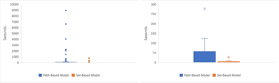
Figure 7: A box plot showing the distribution of solution times (in seconds) of all the 116 instances for the Path-Based Model from [10] and the Set-Based Model. The box plot on the right excludes outliers.

In conclusion, the Set-Based Model is a significant improvement over previous methods. Indeed, it provides optimal solutions in substantially less time, and memory usage for the majority of the instances considered. The same cannot be said about the Set-Based Model when linear relaxations only are considered, as the Path-Based Model can be solved much faster in most cases because of the fewer number of constraints, although it sometimes generates a looser estimate on the value of the optimal integer solution. In terms of memory usage, the Set-Based Model consumes approximately an average of 95MB, with a standard deviation of 132 and median of 41 when solving the instances considered. On the other hand, the Path-Based Model consumes approximately an average of 363MB, with a standard deviation of 486 and median of 116. For considerably large sized instances such as R.700.100.30 and R.700.100.60, the Path-Based Model consumes 1841MB and 1097MB for each of those two instances, whereas the Set-Based Model consumes 263MB and 286MB for the same instances. The two instances considered are solved at the root node of the branch-decision tree by both models.

4.2 Computational Results for the PCMCA-WT

For the computational experiments of the PCMCA-WT, we omit the detailed results for SOPLIB benchmark instances. However, we can draw the following conclusions on these instances. The Multi-Commodity Flow (MCF) model is unable to solve large sized instances because of memory issues (building the model consumes around 5GB of memory on average) or time out while solving the model’s linear relaxation. Since the linear relaxation of MCF model was unable to solve any single instance from SOPLIB benchmark set, we concluded that it is highly unsuitable for solving such instances. The characteristics of SOPLIB instances are summarized in Table 2. The Distance-Accumulation (DA) model and the Adjusted Arc-Cost (AAC) model are able to optimally solve SOPLIB instances with low density precedence graphs within the time limit, with an average of 800 seconds, and achieve an average optimality gap of 63.8% for the LR models and 63.3% for the IP models before timing out for the remaining instances. These figures are much higher compared to the other two benchmark sets as will be shown later. The computational experiments have shown that large-sized instances with a highly dense precedence graph are outside the reach of the models proposed due to the intrinsic complexity of the problem.

Table 1: Overall computational results for comparing the Path-Based Model from [10] and the Set-Based Model for the PCMCA for TSPLIB instances

Instance				Path-Based Model [10]				Set-Based Model
				LR		IP		LR			IP
Name	Size	Density of P	$z^{*}$	Time (s)	Gap	Nodes	Time (s)	Cuts	Time (s)	Gap	Nodes	Cuts	Time (s)
br17.10	18	0.314	25	0.032	0.000	3	0.060	21	0.015	0.000	0	21	0.015
br17.12	18	0.359	25	0.047	0.000	3	0.063	22	0.016	0.000	0	22	0.016
ESC07	9	0.611	1531	0.031	0.000	0	0.031	13	0.031	0.000	0	13	0.031
ESC11	13	0.359	1752	0.031	0.000	0	0.031	1	0.031	0.000	0	1	0.031
ESC12	14	0.396	1138	0.016	0.000	0	0.016	1	0.016	0.000	0	1	0.016
ESC25	27	0.177	1041	0.062	0.000	0	0.062	31	0.063	0.000	0	31	0.063
ESC47	49	0.108	703	0.484	0.284	5	0.469	142	0.547	0.000	0	142	0.547
ESC63	65	0.173	56	0.329	0.000	0	0.329	42	0.218	0.000	0	42	0.218
ESC78	80	0.139	502	0.094	0.000	0	0.094	1	0.047	0.000	0	1	0.047
ft53.1	54	0.082	3917	1.172	0.408	7	1.172	78	0.328	0.230	5	84	0.375
ft53.2	54	0.094	3978	0.281	7.642	104	0.688	57	0.188	2.765	55	211	0.547
ft53.3	54	0.225	4242	1.890	5.587	122	2.547	96	0.453	0.000	0	96	0.453
ft53.4	54	0.604	4882	0.156	2.663	9	0.250	13	0.047	0.000	0	13	0.047
ft70.1	71	0.036	32846	2.891	0.000	1	2.828	158	2.750	0.000	0	158	2.750
ft70.2	71	0.075	32930	2.985	0.035	2	3.016	163	2.719	0.000	0	163	2.719
ft70.3	71	0.142	33431	0.750	2.423	954	63.171	66	0.265	2.034	145	2077	38.250
ft70.4	71	0.589	35179	13.015	0.584	53	13.438	30	0.094	2.146	369	1070	6.281
rbg048a	50	0.444	204	0.047	0.000	0	0.047	5	0.031	0.000	0	5	0.031
rbg050c	52	0.459	191	0.313	0.000	0	0.313	11	0.047	0.000	0	11	0.047
rbg109	111	0.909	256	11.578	0.000	0	11.578	14	0.094	0.000	0	14	0.094
rbg150a	152	0.927	373	2.485	0.000	0	2.485	14	0.187	0.000	1	14	0.219
rbg174a	176	0.929	365	29.610	0.274	2	29.609	22	0.297	0.000	1	22	0.313
rbg253a	255	0.948	375	13.985	0.000	0	13.985	22	1.125	0.000	0	22	1.125
rbg323a	325	0.928	754	1.547	0.000	0	1.547	26	1.047	0.000	0	26	1.047
rbg341a	343	0.937	610	23.344	3.279	376	278.859	89	3.031	0.000	0	89	3.031
rbg358a	360	0.886	595	0.312	0.000	0	0.312	67	5.812	0.000	0	67	5.812
rbg378a	380	0.894	559	16.079	3.936	543	178.515	21	1.829	4.472	36	282	19.047
kro124p.1	101	0.046	32597	0.734	5.997	47	1.844	95	1.782	0.000	0	95	1.782
kro124p.2	101	0.053	32851	0.578	6.929	1433	11.203	109	1.828	0.568	27	238	3.281
kro124p.3	101	0.092	33779	8.672	2.680	258648	6599.140	69	0.844	3.486	98	656	7.469
kro124p.4	101	0.496	37124	41.828	1.375	198	59.359	128	1.672	0.000	0	128	1.672
p43.1	44	0.101	2720	0.594	12.684	238	4.203	68	0.187	10.409	128	692	1.765
p43.2	44	0.126	2720	1.016	8.364	119	1.781	33	0.079	11.029	237	1164	4.359
p43.3	44	0.191	2720	0.547	14.407	283	2.829	77	0.188	7.537	134	598	1.437
p43.4	44	0.164	2820	1.218	8.688	198	3.516	11	0.047	8.333	353	1065	2.797
prob.100	100	0.048	650	11.766	1.308	1428	36.594	1840	622.437	0.240	4	1962	743.969
prob.42	42	0.116	143	0.125	0.000	0	0.125	2	0.032	0.000	0	2	0.032
ry48p.1	49	0.091	13095	0.828	0.886	879	1.656	31	0.094	1.894	54	177	0.609
ry48p.2	49	0.103	13103	1.031	0.551	220	1.593	58	0.235	0.000	0	58	0.235
ry48p.3	49	0.193	13886	2.109	3.657	123233	638.344	34	0.078	6.852	146	634	2.156
ry48p.4	49	0.588	15340	2.531	7.210	8610	24.156	65	0.172	5.847	32	153	0.313
Average				4.808	2.484	9700	194.923	94	15.878	1.655	45	300	20.855

Table 2: Overall computational results for comparing the Path-Based Model from [10] and Set-Based Model for the PCMCA for SOPLIB instances

Instance				Path-Based Model [10]				Set-Based Model
				LR		IP		LR			IP
Name	Size	Density of P	$z^{*}$	Time (s)	Gap	Nodes	Time (s)	Cuts	Time (s)	Gap	Nodes	Cuts	Time (s)
R.200.100.1	200	0.020	29	0.219	0.000	0	0.219	11	0.875	0.000	0	11	0.875
R.200.100.15	200	0.847	454	3235.391	5.740	382	4034.859	85	1.079	13.877	177	2395	64.812
R.200.100.30	200	0.957	529	12.922	11.153	59	54.828	39	0.266	9.263	10	77	0.875
R.200.100.60	200	0.991	6018	3.593	0.000	0	3.593	0	0.094	0.000	0	0	0.094
R.200.1000.1	200	0.020	887	0.203	0.000	0	0.203	3	0.656	0.000	0	3	0.656
R.200.1000.15	200	0.876	5891	203.234	4.261	132	329.313	35	0.766	5.568	87	557	7.860
R.200.1000.30	200	0.958	7653	56.000	0.026	2	57.141	9	0.234	0.000	0	9	0.297
R.200.1000.60	200	0.989	6666	3.797	0.000	0	3.797	0	0.094	0.000	0	0	0.094
R.300.100.1	300	0.013	13	0.500	0.000	0	0.500	14	2.250	0.000	0	14	2.250
R.300.100.15	300	0.905	575	3.985	10.261	87859	2220.656	20	1.171	7.652	139	1111	55.734
R.300.100.30	300	0.970	756	1.672	0.000	0	1.672	27	0.562	0.000	0	27	0.562
R.300.100.60	300	0.994	708	1.531	0.000	2	2.469	2	0.297	0.000	0	2	0.375
R.300.1000.1	300	0.013	715	10.546	0.000	0	10.546	8	2.094	0.000	0	8	2.515
R.300.1000.15	300	0.905	6660	0.812	5.983	3304	91.938	136	2.610	0.811	73	819	16.531
R.300.1000.30	300	0.965	8693	1.531	0.000	0	1.531	6	0.391	0.000	0	6	0.453
R.300.1000.60	300	0.994	7678	23.234	0.000	0	23.234	2	0.297	0.000	0	2	0.297
R.400.100.1	400	0.010	6	0.391	0.000	0	0.391	42	5.781	0.000	2	45	9.750
R.400.100.15	400	0.927	699	0.328	10.837	52858	2021.813	24	0.906	10.014	109	548	44.922
R.400.100.30	400	0.978	712	10.156	0.000	0	10.156	14	1.656	0.000	0	14	2.031
R.400.100.60	400	0.996	557	0.219	0.000	0	0.219	0	0.328	0.000	0	0	0.328
R.400.1000.1	400	0.010	780	6.734	0.000	0	6.734	4	2.797	0.000	0	4	2.797
R.400.1000.15	400	0.930	7382	0.625	8.467	56018	8935.188	78	5.375	2.181	91	362	24.000
R.400.1000.30	400	0.977	9368	34.531	1.057	4797	209.593	20	1.140	4.366	38	97	6.563
R.400.1000.60	400	0.995	7167	2.016	0.000	0	2.016	1	0.500	0.000	0	1	0.500
R.500.100.1	500	0.008	3	217.172	0.000	0	217.172	29	11.812	0.000	0	29	11.812
R.500.100.15	500	0.945	860	1.016	8.488	9879	443.125	100	7.406	3.895	38	286	21.156
R.500.100.30	500	0.980	710	14.453	3.099	11490	696.922	19	0.797	6.620	15	51	3.562
R.500.100.60	500	0.996	566	0.687	0.000	0	0.687	1	0.844	0.000	0	1	0.844
R.500.1000.1	500	0.008	297	0.609	0.000	0	0.609	0	4.469	0.000	0	0	4.469
R.500.1000.15	500	0.940	8063	82.015	0.000	57	100.640	119	15.063	0.000	0	119	15.063
R.500.1000.30	500	0.981	9409	11.141	0.000	0	11.141	11	3.125	0.000	0	11	3.125
R.500.1000.60	500	0.996	6163	0.671	0.000	0	0.671	1	0.875	0.000	0	1	0.875
R.600.100.1	600	0.007	1	659.156	0.000	0	659.156	1455	733.375	0.000	0	1455	733.375
R.600.100.15	600	0.950	568	31.516	0.000	1	34.985	23	5.312	0.000	0	23	5.312
R.600.100.30	600	0.985	776	13.484	1.675	659	298.109	24	2.375	0.000	0	24	2.375
R.600.100.60	600	0.997	538	0.359	0.000	0	0.359	0	0.906	0.000	0	0	0.906
R.600.1000.1	600	0.007	322	0.844	0.000	0	0.844	0	8.625	0.000	0	0	8.625
R.600.1000.15	600	0.945	9763	17.984	2.192	31	159.515	69	12.766	0.000	0	69	12.766
R.600.1000.30	600	0.984	9497	7.219	0.000	0	7.219	13	2.969	0.000	0	13	2.969
R.600.1000.60	600	0.997	6915	0.406	0.000	0	0.406	0	0.922	0.000	0	0	0.922
R.700.100.1	700	0.006	2	1.250	0.000	0	1.250	616	314.875	0.000	0	616	314.875
R.700.100.15	700	0.957	675	41.000	0.000	0	41.000	23	6.875	0.000	0	23	6.875
R.700.100.30	700	0.987	590	3.984	0.000	0	3.984	1	1.25	0.000	0	1	1.250
R.700.100.60	700	0.997	383	0.500	0.000	0	0.500	0	1.422	0.000	0	0	1.422
R.700.1000.1	700	0.006	611	1.625	0.000	0	1.625	0	13.891	0.000	0	0	13.891
R.700.1000.15	700	0.956	2792	1.500	0.000	0	1.500	4	1.875	0.000	0	4	1.875
R.700.1000.30	700	0.986	2658	0.360	0.000	0	0.360	0	0.828	0.000	0	0	0.828
R.700.1000.60	700	0.997	1913	0.515	0.000	0	0.515	0	1.375	0.000	0	0	1.375
Average				98.409	1.526	4740	431.352	64	24.714	1.338	16	184	29.494

Table 3: Overall computational results for comparing the Path-Based Model from [10] and Set-Based Model for the PCMCA for COMPILERS instances

Instance				Path-Based Model [10]				Set-Based Model
				LR		IP		LR			IP
Name	Size	Density of P	$z^{*}$	Time (s)	Gap	Nodes	Time (s)	Cuts	Time (s)	Gap	Nodes	Cuts	Time (s)
gsm.153.124	126	0.970	185	0.578	0.000	0	0.578	49	0.125	1.081	3	53	0.140
gsm.444.350	353	0.990	1542	0.078	0.000	0	0.078	0	0.094	0.000	0	0	0.094
gsm.462.77	79	0.840	292	3.422	0.000	17	4.047	14	0.031	0.000	0	14	0.031
jpeg.1483.25	27	0.484	71	0.234	0.000	43	0.266	21	0.031	0.000	4	34	0.047
jpeg.3184.107	109	0.887	411	14.640	0.487	24	16.844	32	0.093	0.000	0	32	0.093
jpeg.3195.85	87	0.740	13	278.844	38.462	4041	1366.985	45	0.125	38.462	5674	16979	897.312
jpeg.3198.93	95	0.752	140	252.734	2.857	2204	529.781	29	0.141	3.571	401	1686	9.704
jpeg.3203.135	137	0.897	507	47.578	0.394	31	56.703	18	0.094	2.170	7	41	0.125
jpeg.3740.15	17	0.257	33	1.782	3.030	231	0.234	17	0.031	0.000	0	17	0.031
jpeg.4154.36	38	0.633	74	0.641	5.405	1462	2.500	43	0.063	0.000	0	43	0.063
jpeg.4753.54	56	0.769	146	2.766	0.685	11	2.984	38	0.062	0.685	6	59	0.109
susan.248.197	199	0.939	588	76.329	0.340	22	106.672	21	0.125	0.000	0	21	0.125
susan.260.158	160	0.916	472	12.156	1.695	570	123.594	33	0.141	0.000	0	33	0.141
susan.343.182	184	0.936	468	194.188	1.068	776	474.391	47	0.203	0.962	19	89	0.359
typeset.10192.123	125	0.744	241	4.859	10.373	5565	297.859	93	0.500	0.000	0	93	0.500
typeset.10835.26	28	0.349	60	0.063	0.000	0	0.063	14	0.031	0.000	0	14	0.031
typeset.12395.43	45	0.518	125	0.531	0.800	10	0.437	27	0.078	0.000	0	27	0.078
typeset.15087.23	25	0.557	89	0.297	1.124	32	0.297	24	0.047	0.000	0	24	0.047
typeset.15577.36	38	0.555	93	0.031	0.000	0	0.031	4	0.015	0.000	0	4	0.015
typeset.16000.68	70	0.658	67	21.891	0.000	0	21.891	643	3.281	8.955	144	1316	7.172
typeset.1723.25	27	0.245	54	0.203	5.556	7660	4.094	19	0.031	5.556	21	99	0.110
typeset.19972.246	248	0.993	979	0.110	0.000	0	0.110	0	0.062	0.000	0	0	0.062
typeset.4391.240	242	0.981	837	378.172	0.119	46	6.250	18	0.094	0.000	0	18	0.094
typeset.4597.45	47	0.493	133	0.437	0.000	0	0.437	7	0.031	0.000	0	7	0.031
typeset.4724.433	435	0.995	1819	4.000	0.000	0	4.000	8	0.172	0.000	0	8	0.172
typeset.5797.33	35	0.748	93	0.234	0.000	0	0.234	9	0.032	0.000	0	9	0.032
typeset.5881.246	248	0.986	979	191.813	0.306	191	356.218	52	0.343	0.000	0	52	0.343
Average				55.134	2.693	849	125.095	49	0.225	2.276	233	769	33.965

4.2.1 Computational Results for LR Models

Tables 4-5 show the overall results for the linear relaxation of the MILP models proposed for the PCMCA-WT. In all the tables the Cost column reports the value of the objective function. The Gap column indicates the percentage relative difference between the cost of the best known integer solution of the instance ($Cost_{Best}$), and the objective function cost of the model’s linear relaxation ($Cost_{LR}$), computed as $100\cdot\frac{Cost_{Best}-Cost_{LR}}{Cost_{Best}}$. The Cuts column indicates the number of inequalities that are dynamically added to the model, that is inequalities (23) and (44) for each model. The solution information are not reported for instances where the solver times out or runs out of memory before finding the optimal solution.

The linear relaxation of the MCF model has an average optimality gap of 20.22%, and the solver times out before finding the optimal solution for the model’s linear relaxation for instances that are larger than 240. Comparing the results for the DA and AAC models, the first model’s linear relaxation has an average optimality gap of 23.96%, whereas the second model has an average optimaility gap of 23.99% across all the instances. Comparing the number of generated cuts, the AAC model generates 6% less cuts compared to the DA model. We can notice that the DA model finds higher estimates for the optimal integer solution compared to the other two models, however the AAC model finds better estimates on the symmetrical COMPILERS instances which have symmetric costs. Instances where the AAC model and MCF model found tighter estimates are underlined in the tables.

A major problem that we can notice in the MCF model is that the solution times are much larger when compared to the other two models. For example, the MCF model finds the optimal solution of ESC78 instance within 9 minutes compared to 4 and 6 seconds of computing time by the other two models. The same increased solution time can be noticed in other instances, sometimes reaching almost an hour to solve the linear relaxation compared to few seconds. For the instances that are optimally solved by all three LR models, the solution time is on average 889 seconds for the MCF model, 19 seconds for the DA model, and 38 seconds for the AAC model.

In general, it is hard to decide which linear relaxation would perform better on some instances, however the DA model seems to be the most suitable, as its linear relaxation is much easier to solve compared to the other two, and its result exhibits a lower average optimality gap compared to the other two models.

Table 4: LR Models computational results for PCMCA-WT for TSPLIB instances

Instance			MCF			DA				AAC
Name	Size	Density of P	Cost	Time (s)	Gap	Cost	Cuts	Time (s)	Gap	Cost	Cuts	Time (s)	Gap
br17.10	18	0.314	25.08	1.437	42.996	25.17	15	0.265	42.795	25.15	18	0.203	42.841
br17.12	18	0.359	25.12	1.032	42.917	25.17	15	0.265	42.795	25.15	18	0.203	42.841
ESC07	9	0.611	1887.50	0.204	0.971	1890.75	3	0.110	0.800	1782.07	7	0.031	6.502
ESC11	13	0.359	2127.00	0.297	2.162	2067.00	10	0.187	4.922	2040.30	8	0.312	6.150
ESC12	14	0.396	1138.00	0.109	0.000	1138.00	0	0.063	0.000	1138.00	1	0.078	0.000
ESC25	27	0.177	1043.05	3.297	9.927	1082.41	37	0.672	6.528	1064.20	40	0.890	8.100
ESC47	49	0.108	703.14	36.969	5.872	703.12	257	9.250	5.874	703.14	80	3.625	5.871
ESC63	65	0.173	56.00	266.610	0.000	56.00	6	1.594	0.000	56.00	67	20.937	0.000
ESC78	80	0.139	502.16	523.810	58.014	721.93	8	4.453	39.638	718.00	6	5.969	39.967
ft53.1	54	0.082	3953.05	188.391	3.325	3962.45	34	5.594	3.095	3949.66	25	8.297	3.408
ft53.2	54	0.094	3997.50	180.250	6.688	3998.74	40	5.531	6.659	3993.84	52	8.547	6.773
ft53.3	54	0.225	4286.90	171.203	21.442	4388.35	69	7.640	19.583	4249.72	97	13.562	22.124
ft53.4	54	0.604	5026.27	52.062	21.940	5149.40	18	4.875	20.028	5010.26	21	5.250	22.189
ft70.1	71	0.036	32801.04	1021.590	1.492	32980.40	148	16.610	0.954	32851.51	130	39.453	1.341
ft70.2	71	0.075	32895.06	1523.523	4.514	33016.60	160	22.235	4.161	32939.71	171	48.172	4.384
ft70.3	71	0.142	33441.93	2048.220	21.740	33641.84	402	47.500	21.272	33672.54	264	63.344	21.201
ft70.4	71	0.589	35433.67	113.969	12.302	35805.55	132	18.188	11.381	35427.98	156	31.813	12.316
rbg048a	50	0.444	231.57	335.875	11.277	228.06	11	1.703	12.621	221.84	11	3.985	15.004
rbg050c	52	0.459	215.12	124.781	4.393	214.35	36	2.485	4.733	217.24	26	3.422	3.449
rbg109	111	0.909	293.13	590.328	29.196	314.83	19	8.609	23.954	314.79	5	13.531	23.964
rbg150a	152	0.927	373.34	1417.090	30.991	417.14	12	10.969	22.895	416.17	7	32.969	23.074
rbg174a	176	0.929	365.40	2096.480	37.000	405.03	10	21.984	30.167	401.07	9	65.828	30.850
rbg253a	255	0.948	-	-	-	458.28	11	60.750	40.714	467.20	7	248.812	39.560
rbg323a	325	0.928	-	-	-	920.95	23	210.250	77.176	892.63	19	719.109	77.878
rbg341a	343	0.937	-	-	-	677.73	52	365.250	82.165	672.90	44	725.343	82.292
rbg358a	360	0.886	-	-	-	699.25	77	429.547	78.785	666.92	29	1395.735	79.766
rbg378a	380	0.894	-	-	-	644.63	107	422.203	76.635	605.73	61	1787.078	78.045
kro124p.1	101	0.046	32597.08	3482.940	7.476	32657.90	106	47.765	7.304	32603.69	123	89.266	7.457
kro124p.2	101	0.053	32761.06	3482.630	13.687	33053.63	135	48.688	12.916	32922.44	171	134.109	13.262
kro124p.3	101	0.092	33715.31	3490.750	37.550	33951.74	270	76.703	37.112	33826.66	303	212.000	37.344
kro124p.4	101	0.496	37386.23	2552.250	32.255	38025.91	132	35.250	31.096	37233.59	174	88.859	32.532
p43.1	44	0.101	2825.00	864.844	36.801	2825.00	49	2.140	36.801	2797.37	53	3.797	37.419
p43.2	44	0.126	2759.38	1036.547	35.453	2825.00	98	2.672	33.918	2722.91	140	9.422	36.306
p43.3	44	0.191	2759.53	573.968	48.660	2845.00	113	3.469	47.070	2722.79	197	10.407	49.343
p43.4	44	0.164	2925.07	11.937	40.305	2930.08	115	2.984	40.202	2822.27	93	4.968	42.403
prob.100	100	0.048	643.00	3484.390	36.210	668.13	1225	598.594	33.717	657.65	1009	999.453	34.757
prob.42	42	0.116	148.90	57.672	12.927	153.18	107	4.813	10.421	148.26	52	5.469	13.298
ry48p.1	49	0.091	13134.08	99.141	4.285	13133.93	62	4.953	4.286	13115.36	54	8.391	4.421
ry48p.2	49	0.103	13195.09	95.937	9.986	13243.77	48	4.703	9.654	13206.48	34	5.203	9.909
ry48p.3	49	0.193	13926.14	136.859	14.700	13979.71	207	12.469	14.371	13925.41	191	19.016	14.704
ry48p.4	49	0.588	16168.48	16.781	17.713	16316.13	60	5.344	16.962	16186.84	93	9.406	17.620
Average				835.671	19.921		108	61.691	24.784		99	166.982	25.626

Table 5: LR Models computational results for PCMCA-WT for COMPILERS instances

Instance			MCF			DA				AAC
Name	Size	Density of P	Cost	Time (s)	Gap	Cost	Cuts	Time (s)	Gap	Cost	Cuts	Time (s)	Gap
gsm.153.124	126	0.97	221.14	135.500	29.348	222.23	15	0.610	29.000	223.41	15	3.312	28.623
gsm.444.350	353	0.99	-	-	-	1914.83	6	4.531	33.351	2042.75	4	5.156	28.898
gsm.462.77	79	0.84	377.54	231.625	22.636	384.41	27	6.016	21.227	380.96	29	5.375	21.934
jpeg.1483.25	27	0.484	84.00	1.844	3.446	78.97	17	0.406	9.230	76.89	16	0.719	11.621
jpeg.3184.107	109	0.887	419.22	254.187	38.710	441.65	60	2.875	35.431	451.07	76	16.047	34.054
jpeg.3195.85	87	0.74	13.04	3595.590	47.837	9.00	126	7.875	64.000	13.00	195	9.130	48.000
jpeg.3198.93	95	0.752	140.26	3594.700	31.244	151.87	214	9.296	25.554	152.79	152	11.730	25.103
jpeg.3203.135	137	0.897	524.22	1217.125	30.104	564.03	58	3.234	24.796	568.97	122	21.063	24.137
jpeg.3740.15	17	0.257	33.00	0.313	0.000	33.00	5	0.093	0.000	33.00	3	0.125	0.000
jpeg.4154.36	38	0.633	86.88	7.843	3.469	85.06	26	2.125	5.489	84.01	21	0.765	6.656
jpeg.4753.54	56	0.769	150.20	76.875	8.413	153.08	30	3.500	6.659	150.19	40	2.250	8.421
susan.248.197	199	0.939	613.41	3519.028	48.192	658.84	108	9.672	44.355	682.70	138	34.656	42.340
susan.260.158	160	0.916	494.65	1681.391	43.533	519.01	116	7.796	40.752	534.43	244	55.359	38.992
susan.343.182	184	0.936	469.79	1488.110	45.500	539.47	72	6.156	37.416	554.04	94	20.234	35.726
typeset.10192.123	125	0.744	246.52	3579.440	40.599	264.30	131	22.078	36.313	260.60	90	23.328	37.205
typeset.10835.26	28	0.349	93.55	2.187	16.470	81.83	7	0.328	26.938	92.34	9	0.625	17.554
typeset.12395.43	45	0.518	139.02	57.437	4.784	137.85	110	3.094	5.582	137.27	107	4.484	5.979
typeset.15087.23	25	0.557	92.27	2.046	4.878	93.00	13	0.157	4.124	93.00	30	0.516	4.124
typeset.15577.36	38	0.555	120.01	4.141	3.995	120.69	21	0.531	3.448	120.01	14	1.015	3.992
typeset.16000.68	70	0.658	70.00	2051.330	12.500	70.07	121	4.062	12.413	69.48	486	32.735	13.150
typeset.1723.25	27	0.245	56.00	5.516	6.667	55.33	93	1.062	7.783	55.50	90	2.047	7.500
typeset.19972.246	248	0.993	-	-	-	1229.52	4	1.891	36.261	1234.43	11	4.328	36.007
typeset.4391.240	242	0.981	-	-	-	1006.12	31	2.812	28.745	1057.66	64	10.281	25.095
typeset.4597.45	47	0.493	144.01	23.484	7.094	143.13	89	3.282	7.658	141.18	169	9.281	8.916
typeset.4724.433	435	0.995	-	-	-	2351.03	29	12.016	31.517	2351.76	33	21.531	31.495
typeset.5797.33	35	0.748	105.93	2.843	6.258	106.00	9	0.625	6.195	104.21	21	0.891	7.779
typeset.5881.246	248	0.986	-	-	-	1204.29	27	5.234	29.159	1229.51	28	9.422	27.676
Average				978.753	20.713		58	4.495	22.718		85	11.348	21.518

4.2.2 Computational Results for IP Models

Tables 6-7 show the overall results of the MILP models proposed for the PCMCA-WT. In Tables 6-7, the Cost column reports the lower bound ($LB$) and upper bound ($UB$) on the value of the objective function obtained from solving the respective model. The IP Gap column measures the percentage relative difference between the upper and lower bound obtained from solving the respective model, calculated as $100\cdot\frac{UB-LB}{UB}$. Cuts column indicates the number of inequalities that are dynamically added to the model, that is inequalities (23) and (44) for each model. The solution time is not reported in the tables for the instances that are not optimally solved within the time limit. Moreover, the solution information is not reported for instances where it was not possible to solve the model’s linear relaxation (see Tables 4-5).

The MCF model achieves an optimality gap of 29% on average across all the instances it is able to solve, compared to 14% for the DA model, and 15% for the AAC model. We can notice that the solver is finding it difficult to solve the linear relaxation of the MCF model by observing the small number of nodes generated in the time limit for some of the instances, compared to the other two models. However, the MCF model is able to provide the best known solution (underlined in the tables) for 1 out of 68 instances, and the best lower bound for 1 instance.

Comparing the results of the DA and AAC models, we can see that the DA model has an average optimality gap of 19% compared to 21% across all the instances. Furthermore, the DA model solves three extra instances for the TSPLIB instances, while the AAC model solves one extra instance for the COMPILERS instances. For the instances (marked bold in the tables) that are optimally solved by both models, the DA model is 119% faster at solving those instances on average, computed as $100\cdot\frac{T_{DA}-T_{AAC}}{T_{DA}}$, where $T_{DA}$ and $T_{AAC}$ is the average solution time for solving those instances using the $DA$ model and $AAC$ model. Comparing the number of branch-decision-tree nodes generated by the two models, the DA model generates 36% more nodes on average across all the instances, and 10% more nodes on average for the instances that are optimally solved by the two models, The DA model found the best lower bound for 55 out of 68 instances, and better upper bounds for 51 out of 68 instances. On the other hand, the AAC model found tighter lower bounds for 12 out of 68 instances, and better upper bounds for 16 of those instances (underlined in the tables). In general, the DA model performs better than the AAC model, except on symmetrical instances and/or instances with extreme high densities larger than 0.9.

We can conclude that the AAC model is more suitable for symmetrical instances with extreme densities, while the DA model is more suitable for general instances. The MCF finds better bounds compared to the other two models for some instances, however it is not suitable for instances with size larger than 200.

Table 6: IP Models computational results for PCMCA-WT for TSPLIB instances

Instance			MCF				DA					AAC
Name	Size	Density of P	Cost	IP Gap	Nodes	Time (s)	Cost	IP Gap	Nodes	Cuts	Time (s)	Cost	IP Gap	Nodes	Cuts	Time (s)
br17.10	18	0.314	[35, 44]	20.455	192505		[34, 44]	22.727	2767833	3799		[34, 44]	22.727	2074173	3893
br17.12	18	0.359	[35, 44]	20.455	291653		[35, 45]	22.222	3376744	2519		[35, 44]	20.455	2845672	2265
ESC07	9	0.611	1906	0.000	7	0.109	1906	0.000	17	5	0.078	1906	0.000	0	3	0.078
ESC11	13	0.359	2174	0.000	20	0.265	2174	0.000	22	13	0.172	2174	0.000	33	12	0.219
ESC12	14	0.396	1138	0.000	0	0.078	1138	0.000	0	0	0.063	1138	0.000	0	1	0.078
ESC25	27	0.177	1158	0.000	1158	26.625	1158	0.000	1450	698	3.922	1158	0.000	1098	452	4.812
ESC47	49	0.108	747	0.000	2776	3154.14	747	0.000	750	31743	2230.171	[704, 783]	10.089	2	37495
ESC63	65	0.173	[56, 61]	8.197	165		56	0.000	4100	287	53.281	56	0.000	3177	14118	1223.313
ESC78	80	0.139	[922, 1346]	31.501	920		1196	0.000	11177	267	159.093	1196	0.000	15734	943	301.625
ft53.1	54	0.082	[3984, 4089]	2.568	790		4089	0.000	134416	2932	1430.797	4089	0.000	56905	1433	1195.875
ft53.2	54	0.094	[4054, 4659]	12.986	1055		[4135, 4284]	3.478	200163	6053		[4112, 4318]	4.771	57840	8393
ft53.3	54	0.225	[4472, 6071]	26.338	1030		[4623, 5457]	15.283	168357	6749		[4545, 5734]	20.736	92513	5778
ft53.4	54	0.604	[5409, 6871]	21.278	6531		[5657, 6439]	12.145	564462	2361		[5559, 6668]	16.632	340573	1588
ft70.1	71	0.036	[32937, 37078]	11.168	807		[33117, 33298]	0.544	23240	11362		[33128, 33714]	1.738	27834	6322
ft70.2	71	0.075	[33084, 43282]	23.562	408		[33357, 34450]	3.173	11000	13238		[33297, 34713]	4.079	11474	10171
ft70.3	71	0.142	[33693, 66153]	49.068	287		[33914, 42732]	20.636	8574	15867		[33830, 49116]	31.122	9040	11611
ft70.4	71	0.589	[35912, 44507]	19.312	1969		[36517, 40404]	9.620	121796	3615		[36188, 40701]	11.088	78814	3008
rbg048a	50	0.444	[259, 267]	2.996	596		261	0.000	146017	15025	2794.06	[260, 266]	2.256	62610	14794
rbg050c	52	0.459	[225, 236]	4.661	847		225	0.000	1260	326	10.469	225	0.000	24050	432	210.562
rbg109	111	0.909	[320, 699]	54.220	529		[354, 414]	14.493	150506	219		[349, 428]	18.458	85685	601
rbg150a	152	0.927	[403, 972]	58.539	384		[447, 541]	17.375	59431	232		[441, 650]	32.154	34702	618
rbg174a	176	0.929	[400, 1121]	64.318	326		[446, 580]	23.103	42286	302		[441, 627]	29.665	24226	113
rbg253a	255	0.948	-	-	-		[477, 773]	38.292	12700	152		[475, 971]	51.081	5427	231
rbg323a	325	0.928	-	-	-		[926, 4367]	78.796	4536	86		[903, 4035]	77.621	2845	78
rbg341a	343	0.937	-	-	-		[681, 3832]	82.229	3963	116		[680, 3800]	82.105	2300	90
rbg358a	360	0.886	-	-	-		[706, 3296]	78.580	3408	698		[674, 4109]	83.597	1779	144
rbg378a	380	0.894	-	-	-		[649, 2759]	76.477	2831	110		[613, 6701]	90.852	1128	106
kro124p.1	101	0.046	[32598, 45652]	28.595	1		[32858, 35438]	7.280	3389	139		[32827, 35231]	6.824	6926	5724
kro124p.2	101	0.053	[32762, 55265]	40.718	1		[33190, 37956]	12.557	14237	5920		[33163, 38002]	12.734	8410	3458
kro124p.3	101	0.092	[33716, 329579]	89.770	1		[34217, 53988]	36.621	20016	6098		[33991, 77266]	56.008	3313	9747
kro124p.4	101	0.496	[37395, 103491]	63.866	2		[39413, 55187]	28.583	71246	2652		[38269, 62162]	38.437	32120	2746
p43.1	44	0.101	[2825, 4470]	36.801	779		[2827, 4585]	38.342	160185	19944		[2825, 4615]	38.787	51091	11280
p43.2	44	0.126	[2760, 4845]	43.034	430		[2826, 4275]	33.895	162580	18401		[2826, 5025]	43.761	55765	15014
p43.3	44	0.191	[2828, 6955]	59.339	511		[2864, 6105]	53.088	85658	16311		[2847, 5375]	47.033	26582	10567
p43.4	44	0.164	[2991, 5415]	44.765	5826		[3101, 4900]	36.714	875030	2702		[2981, 4970]	40.020	408540	1620
prob.100	100	0.048	[643, 3611]	82.193	1		[674, 1047]	35.626	3718	9961		[661, 1008]	34.425	1533	7323
prob.42	42	0.116	[163, 171]	4.678	2746		171	0.000	112468	7561	945.203	[167, 171]	2.339	157734	11472
ry48p.1	49	0.091	[13278, 15362]	13.566	1339		[13356, 13854]	3.595	158744	8620		[13371, 13722]	2.558	85005	6664
ry48p.2	49	0.103	[13403, 17833]	24.842	585		[13507, 16968]	20.397	82990	10129		[13508, 14659]	7.852	63149	6161
ry48p.3	49	0.193	[13984, 21379]	34.590	773		[14371, 16337]	12.034	70000	8508		[14299, 16326]	12.416	38332	6103
ry48p.4	49	0.588	[16922, 20030]	15.517	10691		[17339, 19649]	11.756	699363	921		[17136, 20915]	18.068	398622	992
Average				28.164	14679			20.723	252211	5772	693.392		23.719	175531	5453	367.070

Table 7: IP Models computational results for PCMCA-WT for COMPILERS instances

Instance			MCF				DA					AAC
Name	Size	Density of P	Cost	IP Gap	Nodes	Time (s)	Cost	IP Gap	Nodes	Cuts	Time (s)	Cost	IP Gap	Nodes	Cuts	Time (s)
gsm.153.124	126	0.97	[234, 331]	29.305	936		[246, 313]	21.406	357665	413		[243, 319]	23.824	270962	405
gsm.444.350	353	0.99	-	-	-		[1996, 2873]	30.526	50228	209		[2103, 2905]	27.608	27606	216
gsm.462.77	79	0.84	[392, 707]	44.554	1150		[396, 493]	19.675	462000	1734		[391, 488]	19.877	185939	2399
jpeg.1483.25	27	0.484	87	0.000	2338	71.61	87	0.000	20708	583	11.254	87	0.000	33035	553	72.907
jpeg.3184.107	109	0.887	[430, 811]	46.979	992		[488, 684]	28.655	315065	1051		[489, 684]	28.509	121292	744
jpeg.3195.85	87	0.74	[14, 76]	81.579	0		[22, 25]	12.000	27085	9849		[21, 30]	30.000	2955	3273
jpeg.3198.93	95	0.752	[141, 353]	60.057	0		[172, 213]	19.249	89431	2584		[161, 204]	21.078	16822	3448
jpeg.3203.135	137	0.897	[535, 1539]	65.237	14		[600, 755]	20.530	179785	2533		[595, 750]	20.667	120417	1332
jpeg.3740.15	17	0.257	33	0.000	0	0.266	33	0.000	0	5	0.093	33	0.000	0	3	0.125
jpeg.4154.36	38	0.633	90	0.000	10271	139.579	90	0.000	15705	461	25.766	90	0.000	4242	298	12.562
jpeg.4753.54	56	0.769	[157, 174]	9.770	1826		[163, 165]	1.212	1128020	1079		164	0.000	594353	911	2231.235
susan.248.197	199	0.939	[614, 3014]	79.628	0		[718, 1184]	39.358	62265	1519		[736, 1353]	45.602	39582	1511
susan.260.158	160	0.916	[498, 2530]	80.316	74		[541, 1149]	52.916	163071	3999		[564, 876]	35.616	49000	1510
susan.343.182	184	0.936	[527, 1433]	63.224	5		[586, 862]	32.019	111339	901		[591, 887]	33.371	55306	1143
typeset.10192.123	125	0.744	[247, 774]	68.088	0		[280, 415]	32.530	92153	3643		[280, 456]	38.596	59000	1924
typeset.10835.26	28	0.349	[99, 114]	13.158	119310		[99, 112]	11.607	986681	7100		[99, 113]	12.389	577573	5961
typeset.12395.43	45	0.518	[141, 148]	4.730	5556		[143, 146]	2.055	392093	4782		[141, 147]	4.082	175106	4776
typeset.15087.23	25	0.557	97	0.000	10917		97	0.000	24721	1082	29.235	97	0.000	13225	759	32.094
typeset.15577.36	38	0.555	125	0.000	12472	1738.422	125	0.000	18600	1467	51.688	125	0.000	106552	3042	834.797
typeset.16000.68	70	0.658	[71, 102]	30.392	2		[77, 86]	10.465	13917	28566		[77, 80]	3.750	29319	6506
typeset.1723.25	27	0.245	60	0.000	682	84.75	60	0.000	1212	281	3.391	60	0.000	5533	481	29.734
typeset.19972.246	248	0.993	-	-	-		[1325, 1963]	32.501	68601	48		[1307, 1929]	32.245	33530	45
typeset.4391.240	242	0.981	-	-	-		[1067, 1419]	24.806	100406	332		[1093, 1412]	22.592	43577	388
typeset.4597.45	47	0.493	[147, 167]	11.976	3247		[150, 155]	3.226	501643	4681		[149, 159]	6.289	107981	3505
typeset.4724.433	435	0.995	-	-	-		[2378, 5376]	55.766	29538	214		[2460, 3433]	28.343	15907	211
typeset.5797.33	35	0.748	113	0.000	2872	100.234	113	0.000	15172	652	24.25	113	0.000	10733	341	24.953
typeset.5881.246	248	0.986	-	-	-		[1258, 1877]	32.978	105414	318		[1305, 1700]	23.235	44716	183
Average				31.318	7848			17.907	197501	2966	20.811		16.951	101639	1699	404.801

5 Conclusions

This work introduces a more scalable model for the PCMCA, and three models for solving the PCMCA-WT. A proof of complexity shows that the two problems fall inside the NP-hard complexity class. The experimental results show that the benchmark instances for the PCMCA could be solved much more efficiently compared to a previously proposed model. Moreover, the results show that the benchmark instances are much harder to solve under the PCMCA-WT settings. In general, large sized instances with dense precedence graphs are outside the reach of the three PCMCA-WT models proposed, therefore further studies to find better formulations for the problem are needed.

The two problems proposed have applications in designing distribution networks for commodities such as oil and gas, where the network is designed in such a way to avoid passing through a certain location when delivering the commodity to another location. Moreover, the delivery can be scheduled to reach certain locations with higher priority first. The Sequential Ordering Problem is a related problem with a wide range of applications in the domains of scheduling and logistics. The two problems proposed can be seen as relaxations of the Sequential Ordering Problem. Therefore, lower bounds for the SOP based on them (or their linear relaxations) could be derived, together with some new valid inequalities. This in turn could have impact on solving the several real-world problems that can be formulated as a Sequential Ordering Problem.

Appendix A The Path-Based model from [10] fails to detect the violation of precedence constraints in fractional solutions

The MILP model previously proposed for the PCMCA in [10], imposes the precedence relationships by propagating a value along every path with end-points $s$ and $t$ for $(s,t)\in R$ in order to detect a precedence violation. The violation is detected if a non-zero value is propagated from $t$ down to $s$. The model sometimes fail to detect a violating path in a fractional solution due to the diminishing propagated values along that path [10]. However, the Set-Based Model proposed in Section 2.2 is able to detect the violation for the same fractional solution. In order to show this, consider the example shown in Figure 8. Referring back to Algorithm 1, we construct the graph $D_{j}$ (consisting of all the vertices of the original graph $G$ excluding the successors of vertex $s$ in the precedence graph $P$), then we compute a minimum $(r,s)$-cut in $D_{j}$, namely cut $[\{s,1,2\},\{r\}]$, which has a value less than 1 in the example. On the other hand in the model proposed in [10] a value of 0 will be propagated down from $t$ to $s$ failing to detect the violating path. The details about how the value is propagated can be found in [10].

Figure 8: Example of a fractional solution that violates the precedence relationship $(s,t)\in R$, and how the violation cannot be detected by the Path-Based Model. The figure on the left shows the fractional solution with the violating path from $t$ to $s$. The figure in the middle shows the value propagated from $t$ to $s$ next to each vertex, where the violation is not detected using the Path-Based Model because a value of 0 is propagated down to vertex $s$ from $t$. The figure on the right shows how the Set-Based Model is able to detect the violating path, since using Algorithm 1 the graph has a minimum $(r,s)$-cut in $D_{j}$ with value less than 1.

References

- [1] N. Ascheuer, N. Jünger, and G. Reinelt. A branch & cut algorithm for the asymmetric traveling salesman problem with precedence constraints. Computational Optimization and Applications, 17(1):61–84, 2000.
- [2] J. Bang-Jensen. Edge-disjoint in- and out-branchings in tournaments and related path problems. Journal of Combinatorial Theory - Series B, 51(1):1–23, 1991.
- [3] K. Bérczi, S. Fujishige, and N. Kamiyama. A linear-time algorithm to find a pair of arc-disjoint spanning in-arborescence and out-arborescence in a directed acyclic graph. Information Processing Letters, 109(23):1227–1231, 2009.
- [4] F. Bock. An algorithm to construct a minimum directed spanning tree in a directed network. Developments in Operations Research, pages 29–44, 1971.
- [5] S. Böcker and F. Rasche. Towards de novo identification of metabolites by analyzing tandem mass spectra. In Seventh European Conference on Computational Biology and Bioinformatics, ECCB 2008, volume 24, pages 49–55. Springer, 2008.
- [6] M.C. Cai, X. Deng, and L. Wang. Minimum k arborescence with bandwidth constraints. Algorithmica, 38(4):529–537, 2004.
- [7] F. Carrabs, R. Cerulli, R. Pentangelo, and A. Raiconi. Minimum spanning tree with conflicting edge pairs: a branch-and-cut approach. Annals of Operations Research, 298:65–78, 2021.
- [8] Y.J. Chu and T.H. Liu. On the shortest arborescence of a directed graph. Scientia Sinica, 14:1396–1400, 1965.
- [9] A. Darmann, U. Pferschy, and J. Schauer. Determining a minimum spanning tree with disjunctive constraints. In Algorithmic Decision Theory, pages 414–423. Springer Berlin Heidelberg, 2009.
- [10] M. Dell’Amico, J. Jamal, and R. Montemanni. A mixed integer linear program for a precedence-constrained minimum-cost arborescence problem. In Proc. The International Conference on Industrial Engineering and Applications (Europe), pages 216–221, 2021.
- [11] J. Edmonds. Optimum branchings. Journal of research of the national bureau of standards, B 71(4):233–240, 1967.
- [12] L.F. Escudero. An inexact algorithm for the sequential ordering problem. European Journal of Operational Research, 37(2):236–249, 1988.
- [13] K.P. Eswaran and R.E. Tarjan. Augmentation problems. SIAM Journal on Computing, 5:653–665, 1976.
- [14] G. Fertin, J. Fradin, and G. Jean. Algorithmic aspects of the maximum colorful arborescence problem. In Theory and Applications of Models of Computation. TAMC 2017, pages 216–230. Springer, 2017.
- [15] M. Fischetti and D. Vigo. A branch-and-cut algorithm for the resource-constrained minimum-weight arborescence problem. Networks: An International Journal, 29(1):55–67, 1997.
- [16] A.M. Frieze and T. Tkocz. A randomly weighted minimum arborescence with a random cost constraint. Mathematics of Operations Research, 2021.
- [17] G. Galbiati, S. Gualandi, and F. Maffioli. On minimum changeover cost arborescences. Lecture Notes in Computer Science, 6630:112–123, 2011.
- [18] M.R. Garey and D.S. Johnson. Computers and intractability: A Guide to the Theory of NP-Completeness. W H Freeman & Co., San Francisco, 1979.
- [19] L. Gouveia and M.J. Lopes. The capacitated minimum spanning tree problem: On improved multistar constraints. European Journal of Operational Research, 160(1):47–62, 2005.
- [20] S.L. Hakimi. Optimum distribution of switching centers in a communication network and some related graph theoretic problems. Operations Research, 13(3):462–475, 1965.
- [21] J.X. Hao and J.B. Orlin. A faster algorithm for finding the minimum cut in a directed graph. Journal of Algorithms, 17(3):424–446, 1994.
- [22] V.R Houndji, P. Schaus, M.N. Hounkonnou, and L. Wolsey. The weighted arborescence constraint. In International Conference on AI and OR Techniques in Constraint Programming for Combinatorial Optimization Problems, pages 185–201. Springer, 2017.
- [23] R. Kawatra and D. Bricker. Design of a degree-constrained minimal spanning tree with unreliable links and node outage costs. European Journal of Operational Research, 156(1):73–82, 2004.
- [24] J. Kováč. Complexity of the path avoiding forbidden pairs problem revisited. Discrete Applied Mathematics, 161(10):1506–1512, 2013.
- [25] J. Li, X. Liu, and J. Lichen. The constrained arborescence augmentation problem in digraphs. In 2017 3rd IEEE International Conference on Computer and Communications (ICCC), pages 1204–1209. IEEE, 2017.
- [26] Y. Li, M.T. Thai, F. Wang, and D. Zhu Du. On the construction of a strongly connected broadcast arborescence with bounded transmission delay. IEEE Transactions on Mobile Computing, 5(10):1460–1470, 2006.
- [27] R. Montemanni, D.H. Smith, and L.M. Gambardella. A heuristic manipulation technique for the sequential ordering problem. Computers & Operations Research, 35(12):3931–3944, 2008.
- [28] R Montemanni, D.H. Smith, A.E. Rizzoli, and L.M. Gambardella. Sequential ordering problems for crane scheduling in port terminals. International Journal of Simulation and Process Modelling, 5(4):348–361, 2009.
- [29] V. Morais, B. Gendron, and G.R. Mateus. The -arborescence star problem: Formulations and exact solution approaches. Computers & Operations Research, 102:91–101, 2019.
- [30] A.H. Pereira, G.R. Mateus, and S. Urrutia. Branch-and-cut algorithms for the -arborescence star problem. International Transactions in Operational Research, 29(4):2374–2400, 2021.
- [31] G. Reinelt. TSPLIB–A travelling salesman problem library. ORSA Journal on Computing, 3(4):376–384, 1991.
- [32] W. Shi and C. Su. The rectilinear steiner arborescence problem is NP-complete. SIAM Journal on Computing, 35(3):729–740, 2005.
- [33] G. Shobaki and J. Jamal. An exact algorithm for the sequential ordeing problem and its application to switching energy minimization in compilers. Computational Optimizations and Applications, 61(2):343–372, 2015.
- [34] L.A. do Carmo Viana and M. Campêlo. Two dependency constrained spanning tree problems. International Transactions in Operational Research, 27(2):867–898, 2020.