Holographic Complexity of LST and Single Trace $T\overline{T},\,J\overline{T}$ and $T\overline{J}$ deformations

Abstract

This work is an extension of our previous work Chakraborty:2020fpt where we exploited holography to compute the complexity characteristics of Little String Theory (LST), a nonlocal, nongravitational field theory which flows to a local 2d CFT in the IR under RG via an integrable irrelevant ($T\overline{T}$) deformation. Here we look at the more general LST obtained by UV deforming the 2d CFT by incorporating Lorentz violating irrelevant $J\overline{T}$ and $T\overline{J}$ deformations on top of $T\overline{T}$ deformation, in an effort to capture the novel signatures of Lorentz violation (on top of nonlocality) on quantum complexity. In anticipation of the fact that the dual field theory is Lorentz violating, we compute the volume complexity in two different Lorentz frames and the comparison is drawn between the results. It turns out that for this system the nonlocality and Lorentz violation effects are inextricably intertwined in the UV divergence structure of the quantum complexity. The coefficients of the divergences carry the signature of Lorentz boost violation. We also compute the subregion complexity which displays a (Hagedorn) phase transition with the transition point being the same as that for the phase transition of entanglement entropy Chakraborty:2020udr . These new results are consistent with our previous work Chakraborty:2020fpt . Null warped AdS₃ is treated as special case of interest.

1 Introduction $\&$ Summary

Our understanding of strongly coupled gauge theories has been revolutionized by the AdS/CFT Maldacena:1997re ; Gubser:1998bc ; Witten:1998qj ; Aharony:1999ti duality (or more generally gauge/gravity duality Itzhaki:1998dd ). Strongly coupled regimes of field theories, once considered beyond the reach of analytical control due to breakdown of coupling constant perturbation theory, are now routinely being investigated by going over to the dual, weakly coupled physical system in weakly curved spacetime (most of the time constructed from the “bottom up” without the need of any details of string theory/M-theory compactifications). Effectively one solves (in most cases numerically) a much easier classical gravity-matter system, i.e. Einstein field equations coupled to classical matter. This “holographic approach” of solving strongly coupled fields theories (with or without gauge fields), has proliferated the use of GR/SUGRA tools in the fields of condensed matter many-body physics Sachdev:2010ch ; McGreevy:2009xe ; Hartnoll:2009sz and QCD Erlich:2005qh ; DaRold:2005mxj ; Karch:2006pv . In fact, the impact of gauge/gravity duality has been far more profound than simply providing a geometric computational toolkit for strongly coupled regimes of field theory. Thinking about how a dual field theory encodes various phenomena on the gravity side, such the emergent holographic (radial) direction, spatial connectivity in/of the bulk, presence of event horizons in the bulk, formation of gravitational singularities in the bulk etc, has led to the realization of the significance of various concepts from the quantum information and computation (QIC) canon which are able to capture aspects of field theory not captured by traditional observables such as correlators of local operators, or even Wilson loop operators. To name a few such concepts: Information geometry and information metrics, Shanon or Von-Neumann entropy Ryu:2006bv ; Hubeny:2007xt and Renyi Dong:2016fnf Entropy, Mutual Information, Tensor networks Swingle:2009bg , Computational Complexity, Fidelity susceptibility, Quantum error correcting codes. Influx of these ideas from QIC has turned out to be a ground-breaking enterprise leading to novel insights which might even have resolved the information paradox Penington:2019npb ; Almheiri:2019hni . Combining insights from complementary approaches such as holography, integrability or supersymmetry based arguments, lattice based approaches and perturbative approaches, we have explored the landscape of local quantum field theories rather comprehensively. However, the landscape of nonlocal quantum field theories is still mostly unexplored. Nonlocal field theories arise in various contexts in high energy physics both as effective or emergent theories (e.g. Namsrai:1986md ) as well fundamental (UV complete) theories (e.g.Sen:2015uaa ), they can be finite Efimov:1969fd (or super-renormalizable) and unitary. We are optimistic that holography will be as productive in demystifying many aspects/properties of nonlocal quantum field theories such as the LST as it has been for enhancing our understanding of strongly coupled regimes of local field theories. Another fact is that holography beyond the traditional asymptotically AdS setting is also little explored. Our hope is that studying set ups such as the LST will help us get an handle on nonperturbative quantum gravity beyond pure AdS asymptotics to flat asymptotics.

Our present understanding of holography is that the bulk spacetime geometry is a representation or form of encoding of the entanglement structure of the dual field theory state VanRaamsdonk:2009ar ; VanRaamsdonk:2010pw . The well known Ryu-Takayanagi (RT) proposal Ryu:2006bv ; Hubeny:2007xt was one of the earliest major piece of evidence to point in this direction (along with Maldacena’s construction Maldacena:2001kr of the eternal Schwarzschild-AdS (SAdS) as a thermally entangled state of two CFTs). Since then an impressive list of quantum entanglement related CFT observables have been related to classical geometric features of the bulk (see e.g.  VanRaamsdonk:2016exw for a review). However, entanglement entropy or other entanglement related concepts such as tensor networks or error-correcting codes are yet to capture the essential features of bulk geometry which lay hidden behind the black hole horizons. Take for instance the case of the Einstein-Rosen Bridge (ERB) behind the black hole horizons. Entanglement entropy saturates in a short time upon reaching thermalization whereas, ER bridge continues to grow linearly with time even after the dual field theory attains thermalization. To explain the ERB growth, Susskind Susskind:2014rva has imported another concept from quantum information theory and added it to the holographic dictionary, namely the computational complexity of the dual CFT state. Complexity is the property associated with the states in the Hilbert space of states of a quantum mechanical system quantifying the difficulty of preparing a state (called the target state), starting from the given reference state. While this is a well defined quantity for discrete systems, like quantum circuits in information theory, it has turned out to be enormously hard to define complexity for the continuous systems described by a QFT. It is fair to say that a precise and unambiguous definition of complexity is still lacking for field theories. In the approach of Nielsen et. al.2005quant.ph..2070N ; 2006Sci…311.1133N a definition of circuit complexity in field theory has been proposed as the minimum number of unitary gates in the space of unitary operators which has a Finsler geometry. The complexity of a target state, with respect to a reference state, is defined to be the geodesic length in a Finsler manifold with suitable cost functions and penalty factors, which acts like Lagrangian in typical variational problem. These cost functions are further required to obey certain conditions such as continuity, positive definiteness and satisfying the triangle inequality etc. Despite this attempt at achieving precision, there is still arbitrariness in the choice of cost functions which fixes the Finsler metric and complexity depends upon the choice of the metric. Several attempts have been made to define complexity in the continuum limit (see e.g. Jefferson:2017sdb ; Chapman:2017rqy ; Khan:2018rzm ; Yang:2018nda ; Molina-Vilaplana:2018sfn ; Hackl:2018ptj ; Bhattacharyya:2018wym ; Guo:2018kzl ; Bhattacharyya:2018bbv ; Yang:2018tpo ; Camargo:2019isp ; Balasubramanian:2019wgd ; Bhattacharyya:2019kvj ; Erdmenger:2020sup ; Bueno:2019ajd ; Chen:2020nlj ; Flory:2020eot ; Flory:2020dja for an incomplete but representative list). However, it is fair to say that as yet there exists neither any universal and unanimous definition of complexity in the continuum limit nor does there exist a complete study of the possible universality classes. In the continuum limit, complexity, even in principle, is a UV divergent quantity because it is defined to within a tolerance ($\epsilon$) with respect to the target state. Demanding more precision of reproducing the target state requires including more gates which leads to a dependence on the inverse tolerance which is a divergent term. Conventionally UV divergent or quantities explicitly dependent on the cutoff in QFT are considered unphysical as their value can be altered by simply altering the UV cutoff. But the characteristic UV cutoff dependence is a feature which seems to be indispensable while defining complexity in QFT.

There are two proposals in holography, each with its own distinct motivation, as to which bulk geometric feature represents the complexity of the dual boundary field theory quantum state. First one prescribes the field theory complexity to be proportional to the volume of the maximal volume spacelike hypersurface in the bulk which terminates at the exact boundary spatial slice on which the boundary quantum state is specified Susskind:2014rva . This is the complexity-volume ($CV$) proposal. The second proposal Brown:2015bva ; Brown:2015lvg prescribes the complexity to be proportional to the on-shell bulk SUGRA action integral supported over the Wheeler-deWitt (WdW) patch of the boundary spatial slice on which the field theory state is specified. This is the complexity-action ($CA$) proposal. Since the bulk is noncompact, both these bulk geometric duals of complexity are manifestly UV divergent, hence regularization is necessary as the lore goes in holography. In the CV proposal there is an ambiguity - in order to make the expression dimensionless one must include a length scale, $L$, characteristic of the geometry for which there is no unique candidate. For the CA proposal, there are also couple of issues. Some boundaries of the WdW patch are codimension one null submanifolds with edges or joints. The presence of such null boundaries and their joints (edges) requires the inclusion of carefully defined GHY boundary terms as discussed in Lehner:2016vdi . In this paper, we take an alternative approach to this issue Brown:2015lvg ; Parattu:2015gga ; Bolognesi:2018ion . Since we have to regulate the WdW patch in any case, we use a special regularization which deforms the WdW null boundary to timelike and in the process also smooths out the joints. At the end the regulator is removed. In this way we can compute the GHY terms and obtain a UV-regulated result in one go.

In a recent work Chakraborty:2020fpt we focused our attention on the decoupled regime of the theory of a stack of large number ($k\gg 1$) of NS$5$ branes wrapping $T^{4}\times S^{1}$, the so called Little String theory (LST) in $1+1$ dimensions. This system is unlike the theory of a stack of D$p$ branes, since the worldvolume theory living on the NS$5$ branes decouples from the bulk at finite value of the string length $l_{s}=\sqrt{\alpha^{\prime}}$. This implies that this decoupled theory, namely LST living on the NS$5$ branes, still retains stringy nonlocality and is not a local quantum field theory. In fact this decoupled theory living on the NS$5$ branes is to some extent intermediate between string theory (which is nonlocal theory containing massless gravitons) and a local QFT. The dual holographic background is then obtained by taking the near horizon geometry of the NS$5$ branes - it is a metrically flat spacetime with a linear dilaton $\mathbb{R}^{1,1}\times\mathbb{R}_{\phi}$ turned on all the way to spatial infinity. Such a holographic duality has been studied quite extensively in the past Aharony:1998ub ; Kutasov:2001uf . Now if one introduces $p\gg 1$ F$1$ strings wrapping a $S^{1}$ along the NS$5$ directions, the near horizon geometry of the F$1$ strings is given by AdS₃. Thus the full geometry interpolates between AdS₃ in the IR (which corresponds to the near horizon geometry of the F$1$ strings) to flat spacetime with a linear dilaton in the UV (which corresponds to the near horizon geometry of just the NS$5$ branes). Correspondingly, the boundary field theory interpolates between a local CFT₂ dual to AdS₃ in the IR to LST in the UV. The interpolating geometry discussed above is often referred to in the literature as $\mathcal{M}_{3}$. In the wake of the recent developments in the subject of $T\overline{T}$ deformation Smirnov:2016lqw ; Cavaglia:2016oda , it was proposed in Giveon:2017nie that there exists an analogous deformation of string theory in $AdS_{3}$ that shares many properties in common with the double trace $T\overline{T}$ deformation.This is often referred to as the single trace $T\overline{T}$ deformation in the literature which changes the UV asymptotics of the bulk geometry from $AdS_{3}$ to flat spacetime with a linear dilaton keeping fix the IR regime of the geometry. Analysis in Giveon:2017nie shows that the dual background geometry interpolates between $AdS_{3}$ in the IR to flat spacetime with a linear dilaton in the UV. Holography in this background (often referred to as $\mathcal{M}_{3}$) can be realized as a concrete example of holography in non-AdS background that is smoothly connected to $AdS_{3}$. Naturally this non-AdS holography set up has attracted a lot of attention and there has been a lot of studies where holography has been exploited to investigate various aspects of nonlocal field theories such as LST which admit gravity duals, e.g. Asrat:2017tzd ; Chakraborty:2018kpr ; Chakraborty:2018aji ; Chakraborty:2020xyz ; Chakraborty:2020udr ; Chakraborty:2020yka . In our recent work Chakraborty:2020fpt we probed this theory using holographic complexity as a probe. There we computed the volume and action complexity, both at zero and finite temperature. The complexity expressions contained imprints of the stringy nonlocality on the UV divergence structure. To be specific, we encountered quadratic and logarithmic divergences, evidently not to be associated with local field theory in $1$ space dimension (where we expect a linear divergence) when the UV cutoff is smaller than the (Hagedorn) length scale, $\beta_{H}=2\pi l_{s}\sqrt{k\,\lambda}$, set by the $T\overline{T}$ coupling $\lambda$). When the UV cutoff is held larger than the Hagedorn scale, complexity displays a linear UV divergence, much akin to a local field theory in $1$ space dimension. For completeness we computed the holographic complexity at finite temperature as well, however no unanticipated newer type of UV divergences were encountered in perturbation theory around zero temperature.

The purpose of this paper is to extend the our work in Chakraborty:2020fpt to a more general linear combination of irrelevant single trace deformations, namely the single trace $T\overline{T}$,$J\overline{T}$ and $T\overline{J}$ of a CFT₂ which contains/involves conserved left (right)-moving current $J(\overline{J})$. These irrelevant deformations drive the UV theory to nonlocality, in the sense that the UV is not a local fixed point as the high energy density of states exhibits a exponential Hagedorn growth Chakraborty:2020xyz . Moreover, the effect of turning on the irrelevant current $J(\overline{J})$ couplings is to explicitly break Lorentz boost symmetry in the UV. The dual gravity (string) background was introduced in Chakraborty:2019mdf ; Chakraborty:2020cgo which interpolates between AdS₃ in the IR to a linear dilaton background in the UV. From the string viewpoint, the UV is the near horizon limit of the stack of $k$ NS$5$ branes with $p$ F$1$ strings propagating in the world volume while incorporating NS-NS $H$-flux along the world volume directions violating Lorentz boost invariance Chakraborty:2019mdf ; Chakraborty:2018vja ; Apolo:2018qpq . Our main motivation to investigate this set up is to capture the imprint of Lorentz boost symmetry violation in the holographic complexity, to be specific in the UV divergence structure of holographic complexity. In particular, we are interested in finding out whether the imprints of Lorentz symmetry violation and nonlocality on the UV divergence are separate or different kind. Also since the theory does not respect boost symmetry, we would like to know how the UV divergences in complexity change as we move from one Lorentz frame to another. Another motivation of the present work is to study subsystem holographic complexity Alishahiha:2015rta ; Ben-Ami:2016qex ; Carmi:2016wjl which we had omitted in our previous work Chakraborty:2020fpt . Subsystem complexity, just like entanglement entropy of a subsystem’s reduced density matrix is expected to display phase transitions as the subsystem size is tuned. In particular, in the work Chakraborty:2020udr , which looked at entanglement entropy of this system, namely the $T\overline{T}$,$J\overline{T}$ and $T\overline{J}$ deformed CFT₂, entanglement entropy undergoes a (Hagedorn) phase transition when the subsystem size is tuned to a critical spatial size determined by the strength of the irrelevant couplings.

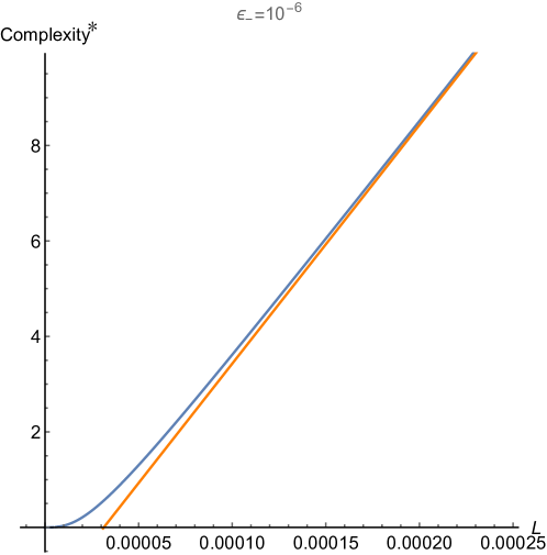
Figure 5: Subregion Volume Complexity vs $L$ plot for null warped AdS₃. For this plot we have set $k=10^{4}$, $l_{s}=10^{-2}$ and $\epsilon=10^{-5}$. Here, the $y$-axis represents $Complexity^{*}=Complexity\times 8\pi G_{N}$ while the $x$-axis is the subregion size $L$ in units of the AdS radius ($\sqrt{k}l_{s}=1.0$). The orange curve is the plot for pure AdS₃ while the blue curve is the plot for null WAdS₃.

The plan of the paper is as follows. In section 2, we give a briefly recap aspects of string theory in $AdS_{3}$, its single trace $T\overline{T},J\overline{T},T\overline{J}$ deformations and highlight interesting features of LST for the sake of completeness. We also review some features of the dual holographic background (bulk). In this regard we would like to point out that one may work with either a $3+1$-dimensional bulk as was done in the works on entanglement entropy Chakraborty:2020udr , or equivalently one can perform a KK reduction on the $y$ circle fiber and work with an effective bulk background in $2+1$ dimensions Chakraborty:2019mdf . Here we take the second approach because it affords us performing immediate comparision or checks with our previous work Chakraborty:2020fpt at every step. In section 3, we set out to compute the holographic complexity of the $T\overline{T},J\overline{T},T\overline{J}$ deformed CFT₂ by implementing the $CV$ prescription in two distinct (boundary) Lorentz frames, which we dub as the stationary frame and static frame (for reasons which will become obvious), related to each other by a Lorentz boost. In either frame, the volume complexity diverges quadratically with a subleading logarithmic divergence. However, anticipated, due to lack of boost symmetry, the coefficients of the quadratic and logarithmic divergence differ in the two frames (and even the finite piece differs). We find that the Lorentz violation effects (governed by the parameter $\epsilon_{\pm}$) and nonlocality effects (governed by the parameter $\lambda$) are inextricably linked - the UV divergence structure depends on a single parameter, namely $\mu=\lambda-\left(\epsilon_{+}+\epsilon_{-}\right)^{2}$ in the stationary frame, and the parameter $\lambda^{\prime}\equiv\lambda-4\epsilon_{+}\epsilon_{-}$ in the static frame. There is no way to cleanly separate the effects of nonlocality and Lorentz boost asymmetry. This is perhaps mildly disappointing since our hope was to be able to see the effects of nonlocality and Lorentz violation in separate or independent UV divergence structures. These results are consistent with the results obtained in Chakraborty:2020fpt - setting $\epsilon_{\pm}=0$ reproduces the volume complexity of the LST dual to the $\mathcal{M}_{3}$ geometry. The quadratic and logarithmic divergences of the volume complexity immediately reveals the nonlocal nature of the dual field theory (LST) as for a local theory the complexity is expected to scale with volume $\mathcal{V}$ (here length) and hence should diverge as lattice cell volume inverse $\mathcal{V}/\epsilon^{d}$. In either frames, the nonlocality scale is set by the respective Hagedorn length $\rho_{H}\propto\sqrt{k\mu}\,l_{s}$ in the stationary frame and $\beta^{\prime}_{H}\propto\sqrt{k\,\lambda^{\prime}}\,l_{s}$ in the static frame. When the lattice spacing is larger than the Hagedorn length scales in the respective frame ($\epsilon\gg\rho_{H}$ or $\epsilon\gg\beta^{\prime}_{H}$), the complexity expression reduces to that of a local field theory with a linear divergence (volume scaling). However if the lattice spacing is shorter than the Hagedorn length scale $\epsilon\ll\rho_{H},$ or $\epsilon\ll\lambda^{\prime}_{H}$, stringy physics takes over and the theory departs from behaving like a local field theory. Finally we note that the logarithmic divergent pieces (subleading divergence) in the complexity expressions in either frame which are accompanied by a dimensionless universal constant coefficient. This coefficient can be given the interpretation of the total number of “regularized/effective” degrees of freedom in the spacetime theory in the nonlocal stringy regime as opposed to the true degrees of freedom of LST which naively diverges Barbon:2008ut ; Chakraborty:2018kpr . Next in Sec. 4, we proceed to evaluate the subregion complexity, in both the stationary (Sec. 4.3) and static (Sec. 4.4) frames. The exact results for subregion complexity are obtained numerically, and the results are displayed graphically, subregion complexity plotted as function of the subregion size, $\mathcal{C}_{V}$ vs $L$ for several different choices of the set of parameters $\lambda,\epsilon_{\pm}$. In either frame, the plots clearly show the Hagedorn phase transition - at a critical subregion size, $L_{c}={\pi\sqrt{k\lambda\lambda^{\prime}}l_{s}\over 2\sqrt{\mu}}$ in the stationary frame and $L^{\prime}_{c}={1\over 2}\pi\sqrt{k\lambda}l_{s}$ in the static frame. For subregion sizes larger than the critical size, the subregion complexity grows linearly with subregion size (length), characteristic of a CFT₂ while for subregion sizes lower than the critical subregion length, subregion complexity grows quadratically with subsystem size (length), which is more like a nonlocal LST. The reason we identify this transition as the Hagedorn transition because the critical length, read off from the numerics (plot), is identical to the phase transition point of entanglement entropy Chakraborty:2020udr ! The fact that the critical length is different in the two frames related by a Lorentz boost simply reflects the boost asymmetry of the LST. In Sec. 5 we explore a very interesting special point in the parameter space of the couplings, namely when $\lambda=\epsilon_{+}=0$ (or $\lambda=\epsilon_{-}=0$) which is dual to the null warped AdS₃ geometry (with nonvanishing dilaton and NS-NS $B$ field). Although this might appear to be a slight digression, we explore this case since this falls under the same broader umbrella of sting theory in AdS₃. Since this limit is singular, instead of naively taking this limit in the final complexity expression of the general case, and redo some of the intermediate steps. The complexity is only well defined (real) when the UV cut off is restricted $\epsilon\leq\sqrt{k}\epsilon_{-}l_{s}$, a trait which lends support to the claims in the literature that the null warped AdS₃ spacetime is the holographic dual to field theory which does not possess a UV completion. For the null WAdS₃, the UV divergence structure is also special, one obtains UV divergences to all orders! In other words the complexity is not an analytic function of the UV cut off. This alludes to the fact that the boundary theory is highly nonlocal (and does not possess boost symmetry either). We also compute the subregion complexity numerically for a boundary interval of length, $L$ and present our results graphically via subregion $C_{V}$ vs $L$ plot in Fig. 5 for a (allowable) range of the warping parameter $\epsilon_{-}$. The subregion complexity monotonically increases with the subregion size and approaches the subregion complexity of a CFT₂ (i.e. pure AdS₃ linear regime) as $L$ is progressively increased. However, unlike what we found for the case of general values of the couplings $\lambda,\epsilon_{\pm}$, there is no Hagedorn like phase transition. These results were obtained in the stationary frame, and there is no static frame for this case since the associated boost transformation which takes one from the stationary to static frame, becomes singular. Next, in Sec. 6 we set out to compute the action complexity for the LST (i.e. the $T\overline{T},J\overline{T},T\overline{J}$ deformed CFT₂). Here we realize that the construction of null surfaces bounding the so called Wheeler-de Witt (WdW) patch is simplest in the boosted frame in the boundary since it leads to a static metric in the bulk. So we exclusively stick to this coordinate system for the entire section/calculation. We leave the construction of lightsheets associated with the WdW patch and the subsequent evaluation of the action-complexity for the stationary frame for future work. While computing the WdW we are confronted with a choice, either to the use the $3+1$-d bulk geometry or to work with the $2+1$-d bulk geometry by dimensionally reducing over the $y$-fiber. Although we present the calculation performed in the dimensionally reduced $2+1$-d set up, pleasantly the action complexities obtained using the the $3+1$-d and $2+1$-d bulk actions agree provided we retain the total derivative terms in the lower dimensional action one gets while performing a dimensional reduction. Usually such total derivative terms are omitted from the dimensionally reduced action as they do not contribute to the equations of motion, but they do contribute to (action) complexity. The action complexity results display the exact same divergence structures, quadratic and logarithm when $\epsilon\ll\beta^{\prime}_{H}$. Modulo an overall constant (courtesy the ambiguity in the choice of the “characteristic length-scale of the geometry” in the definition of the volume complexity), the leading quadratic divergence piece matches for both the volume and action complexities. However we find that the subleading logarithmic divergence, while having the same magnitude in both prescriptions, differs by a sign in the volume and action complexity expressions. This is not a total surprise. Past studies have revealed that the coefficients of the subleading divergent pieces might be different Bolognesi:2018ion hinting to the fact that the two bulk/holographic prescriptions of complexity might actually correspond to different schemes of defining complexity in the boundary field theory. These are also consistent with the results of our previous paper Chakraborty:2020fpt . As a final check, we extract the behavior of the action complexity in the deep IR limit (i.e. $\epsilon\gg\beta^{\prime}_{H}$) where it indeed reproduces the pure AdS₃ or CFT₂ vacuum state complexity Reynolds:2016rvl ; Carmi:2016wjl (for both prescriptions). In Sec. 7, we revisit the null Warped AdS₃ background (with dilaton and B-field) located at point in the coupling space, $\lambda=\epsilon_{+}=0$ and compute the action complexity of dual WCFT₂ using this bulk background. As remarked before, the static frame does not exist for this case, on cannot obtain the results by simply plugging $\lambda=\epsilon_{+}=0$ in the results of Sec. 6. We to tackle the calculation in the stationary frame itself where the construction of the WdW patch boundaries is more complicated than for a static geometry (but far simpler than that for the more general $\lambda,\epsilon_{+}\neq 0$ case). We find that the action complexity null warped AdS₃ vanishes! We believe this is purely a dimensional accident, the action complexity for pure AdS_d+1 analogously vanishes Reynolds:2016rvl ; Chakraborty:2020fpt due to an overall factor of $(d-2)$. Finally, in section 8 we conclude by discussing our results and provide an outlook for future work. In the appendices, we gather some results for ready references in the main sections. In Appendix A we recap the sigma model with the $T\overline{T},J\overline{T},T\overline{J}$ deformations and the $4$d target spacetime which follows and work out the action complexity terms for the $4$d geometry. Next in Appendix B we recap the KK reduction over the $y$ circle fiber following the conventions of Chakraborty:2019mdf , and obtain the dimensionally reduced 3d metric, Dilaton, B-field and KK scalar and KK gauge fields (the KK gauge fields obtained after reducing the 4d NS-NS B-field were missing in Chakraborty:2019mdf . Subsequently we demonstrate the action complexity integrals for the $3$d background work out to be the same as those from the $4$d background worked out in the previous section provided we retain the total derivative terms in the $3$d action. In Appendix C we compute the new GHY term contribution as a result of keeping the total derivative term in the $3$d lagrangian (action) and the net GHY contribution. In Appendix D we compute the holographic entanglement entropy for the WCFT dual to null warped AdS₃, for a boundary interval of size $L$, thereby closing a gap in the literature. For null WCFT we find that the entanglement entropy is log divergent, just like that of an local CFT₂, but the coefficient of the log divergence (central charge) now depends on the warping parameter.

For other interesting works on complexity in the context of double trace $T\overline{T}$ deformed CFT see Akhavan:2018wla ; Jafari:2019qns ; Geng:2019yxo .

2 Review of string theory in AdS₃, single trace $T\overline{T}$ and LST

We first consider critical superstring background AdS${}_{3}\times\mathcal{M}$, with $\mathcal{M}$ being a compact seven dimensional spacelike manifold, which preserves $\mathcal{N}\geq 2$ supersymmetry. A classic example of this kind of a set up consists of type $II$ strings on AdS${}_{3}\times S^{3}\times T^{4}$ preserving $(4,4)$ supersymmetry. The worldsheet theory of strings propagating in AdS₃ with NS-NS fluxes switched on but R-R fluxes turned off is a WZW nonlinear sigma model of the noncompact group manifold $SL(2,\mathbb{R})$. The worldsheet theory is symmetric under the holomorphic (left moving) and antiholomorphic (right moving) components of $sl(2,\mathbb{R})$ current algebra with level $k$. The AdS radius , $R_{AdS}$, is related to the level of the current algebra by the relation $R_{AdS}=\sqrt{k}l_{s}$, $l_{s}=\sqrt{\alpha^{\prime}}$ being the string length.

According to the AdS/CFT correspondence, string theory on (asymptotically) AdS₃ is dual to a two-dimensional CFT living on the conformal boundary of AdS₃. For supergravity approximation to be valid, we will have to work in the parameter regime $k\gg 1$. In the presence of the NS-NS three form H-flux, the spacetime theory has the following properties:

1. The spacetime theory has a normalizable $SL(2,\mathbb{C})$ invariant vacuum state:

   • The NS vacuum, which corresponds to global AdS₃ as the bulk.

   • The R vacuum, that corresponds to massless spinless ($M=J=0$) BTZ as the bulk.

2. The NS sector consists of a sequence of discrete states coming from the discrete series representation of $SL(2,\mathbb{R})$ followed by a continuum of long strings. The continuum starts above a gap of order ${k\over 2}$ Maldacena:2000hw .

3. The R-sector states contain a continuum above a gap of order ${1\over k}$. Here the fate of the discrete series states is unclear.

In the discussion that follows, we focus exclusively on the long strings of the R-sector.

In Seiberg:1999xz , it was argued, that for string theory on AdS${}_{3}\times\mathcal{M}$, the theory supported on a single long string is described by a sigma model on

$$\mathcal{M}^{(L)}_{6k}=\mathbb{R}_{\phi}\times\mathcal{M}~{},$$ (1)

with central charge $6k$. The theory on $\mathbb{R}_{\phi}$ has a dilaton field $\Phi$ that is linear in the coordinate $\phi$ with a slope given by

$$Q^{(L)}=(k-1)\sqrt{{2\over k}}~{}.$$ (2)

Thus the theory on the long string worldsheet has an effective interaction strength given by ${\rm exp}({Q^{(L)}\phi})$ and as a result the dynamics of the long strings becomes strongly coupled as they approach spatial infinity (boundary). But there is a wide range of positions on the radial direction where the long strings are weakly coupled. A natural question that one may ask at this point is: what is the full boundary theory dual to string theory in $AdS_{3}$. The answer to that question, for generic $k$, is unknown, but there are strong evidences to convince that the theory on the long strings is described by the symmetric product CFT

$$(\mathcal{M}^{(L)}_{6k})^{p}/S_{p}~{},$$ (3)

where $p$ represents the number of fundamental (F1) strings that form the background.

String theory in AdS₃ admits an operator $D(x,\overline{x})$ Kutasov:1999xu (where $x$ and $\overline{x}$ are coordinates of the two-dimensional spacetime theory), in the long string sector that has many properties in common with the $T\overline{T}$ operator. For example $D(x,\overline{x})$ is a $(2,2)$ quasi-primary operator of the spacetime Virasoro and has the same OPE with the stress tensor as the $T\overline{T}$ operator. However, there is an important difference between the $T\overline{T}$ operator and the operator $D(x,\overline{x})$: $T\overline{T}$ is a double trace whereas $D(x,\overline{x})$ is single trace. In fact

$$D(x,\overline{x})=\sum_{i=1}^{p}T_{i}\overline{T}_{i}~{},$$ (4)

where $T_{i}\overline{T}_{i}$ can be thought of as the $T\overline{T}$ operator of the $i^{th}$ block $\mathcal{M}^{(L)}_{6k}$ in the symmetric product CFT $(\mathcal{M}^{(L)}_{6k})^{p}/S_{p}$. For an elaborate discussion along this line see Chakraborty:2019mdf ; Chakraborty:2018vja

Next, consider the deformation of the long string symmetric product by the operator $D(x,\overline{x})$. This deforms the $i^{th}$ block CFT $\mathcal{M}^{(L)}_{6k}$ by the operator $T_{i}\overline{T}_{i}$ and is subsequently symmetrized. Such a deformation is evidently irrelevant and it involves flowing up the renormalization group (RG) trajectory. This $D(x,\overline{x})$ deformation of the spacetime theory translates to turning on the worldsheet a truly marginal deformation:

$$\int_{(\mathcal{M}^{(L)}_{6k})^{p}/S_{p}}d^{2}xD(x,\overline{x})\sim\int_{\Sigma}d^{2}zJ_{SL}^{-}\overline{J}_{SL}^{-}~{},$$ (5)

where $z,\overline{z}$ are the complex coordinates of the worldsheet Riemann surface $\Sigma$, $J_{SL}^{-}$ and $\overline{J}_{SL}^{-}$ are respectively the left and right moving null $sl(2,\mathbb{R})$ currents of the worldsheet theory.

The above current-anti-current deformation of the worldsheet $\sigma-$model is exactly solvable, and standard worldsheet techniques yield the metric (in string frame), dilaton and the B-field as Forste:1994wp ; Israel:2003ry

$$\begin{split}&ds^{2}=f^{-1}(-dt^{2}+dx^{2})+kl_{s}^{2}{dU^{2}\over U^{2}}~{},\\ &e^{2\Phi}={g_{s}^{2}\over kU^{2}}f^{-1}~{},\\ &dB={2i\over k^{3/2}\,l_{s}\,U^{2}}f^{-1}\epsilon_{3}~{},\end{split}$$ (6)

where $f=\lambda+{1\over kU^{2}}$, $\lambda$ is the dimensionless coupling of the marginal worldsheet deformation and $g_{s}$ is the asymptotic string coupling in $AdS_{3}$ with $g_{s}^{2}=e^{2\Phi(U\to 0)}\equiv e^{2\Phi_{0}}$. This background is popularly known as $\mathcal{M}_{3}$. The background $\mathcal{M}_{3}$ (LABEL:M3) interpolates between $AdS_{3}$ in the IR (i.e. $U\ll 1/\sqrt{k\lambda}$) to flat spacetime with a linear dilaton, $\mathbb{R}^{1,1}\times\mathbb{R}_{\phi}$ in the UV (i.e. $U\gg 1/\sqrt{k\lambda}$). The coupling $\lambda$ sets the scale at which the transition happens.

The deformed sigma model background (LABEL:M3) can also be obtained as a solution to the equations of the motion of three dimensional supergravity action Giveon:2005mi ; Chakraborty:2020yka

$$S={1\over 16\pi G_{N}}\int d^{3}X\sqrt{-g}e^{-2(\Phi-\Phi_{0})}\left(R+4g^{\mu\nu}\partial_{\mu}\Phi\partial_{\nu}\Phi-{1\over 12}H^{2}-4\Lambda\right)~{},$$ (7)

where $G_{N}$ is the three-dimensional Newton’s constant in $AdS_{3}$, $g_{\mu\nu}$ is the string frame metric, $R$ is the Ricci scalar (in string frame), $\Phi$ is the dilaton, $H=dB$ is the 3-form flux and $\Lambda$ is the cosmological constant.

As an example, the above construction can be realized as follows. Let us consider a stack of $k$ NS5 branes in flat space wrapping a four dimensional compact manifold (e.g. $T^{4}$ or $K_{3}$). The near horizon geometry of the stack of $k$ NS5 branes is given by $\mathbb{R}^{1,1}\times\mathbb{R}_{\phi}$ with a dilaton that is linear in the radial coordinate $\phi$ (where $\phi=\log(\sqrt{k}U)$). The string coupling goes to zero near the boundary (i.e. $U\to\infty$) whereas it grows unboundedly as one goes deep in the bulk (i.e. $U\to 0$). Next, let’s add $p$ (with $p\gg 1$) F1 strings stretched along $\mathbb{R}^{1,1}$. This stabilizes the dilaton and the string coupling saturates as $g_{s}\sim 1/\sqrt{p}$. Thus for large $p$ the string coupling is weak and one can trust string perturbation theory. The F1 strings modifies the IR geometry (i.e. $U\ll 1/\sqrt{k\lambda}$) to $AdS_{3}$. The smooth interpolation between $\mathbb{R}^{1,1}\times\mathbb{R}_{\phi}$ in the UV to $AdS_{3}$ in the IR corresponds to interpolation between near horizon geometry of the NS5 brane system to that of the F1 strings Chakraborty:2020swe ; Chakraborty:2020yka . The spacetime theory interpolates between a CFT₂ with central charge $6kp$ in the IR to two-dimensional LST in the UV. The theory is nonlocal in the sense that the short distance physics is not governed by a fixed point.

LST can be realized as the decoupled theory on the NS5 branes. It has properties that are somewhat intermediate between a local quantum field theory and a full fledged critical string theory. Unlike a local field theory, at high energy $E$, LST has a Hagedorn density of states $\rho\sim e^{\beta_{H}E}$ where $\beta_{H}=2\pi l_{s}\sqrt{k\lambda}$. On the other hand, LST has well defined off-shell amplitudes Aharony:2004xn and upon quantization it doesn’t give rise to massless spin 2 excitation. Both these properties are very similar to local quantum field theories. For a detailed review of LST see Aharony:1998ub ; Kutasov:2001uf .

One can generalize this scenario further by turning on holomorphic and antiholomorphic currents in the spacetime theory $J(x),\overline{J}(\overline{x}))$ Chakraborty:2019mdf ; Kutasov:1999xu . In that case, parallel to the construction of $D(x,\overline{x})$, one can also construct single trace operators, namely, $A(x,\overline{x})$ and $\overline{A}(x,\overline{x})$ of dimension $(1,2)$ and $(2,1)$ respectively Kutasov:1999xu . $A(x,\overline{x})$ has the same conformal dimension and OPE’s with the currents as the irrelevant double trace $J(x)\overline{T}(\overline{x})$ operator. Analogously, the single trace marginal $\overline{A}(x,\overline{x})$ is related to the irrelevant double trace $T(x)\overline{J}(\overline{x})$ operator in the spacetime CFT. In the symmetric product CFT, one can think of the operator of $A,\overline{A}$ as

$$A(x,\overline{x})=\sum_{j=1}^{p}J_{j}(x)\,\overline{T}_{j}(\overline{x});\,\overline{A}(x,\overline{x})=\sum_{j=1}^{p}T_{j}(x)\,\overline{J}_{j}(\overline{x}).$$ (8)

Turning on $A,\overline{A}(x,\overline{x})$, in addition to the $D(x,\overline{x})$ operators, in the spacetime corresponds to the perturbing the worldsheet llagrangian by the following marginal operators,

$$\delta\mathcal{L}_{WS}=\lambda\,J^{-}_{SL}(z)\overline{J}_{SL}^{-}(\overline{z})+\epsilon_{+}\,K(z)\overline{J}_{SL}^{-}(\overline{z})+\epsilon_{-}\,J_{SL}^{-}(z)\overline{K}(\overline{z}).$$ (9)

One has to strictly consider the positive sign of the coupling $\lambda$ because only for that sign of the coupling the spectrum of the deformed theory is real and the theory is unitary.

The worldsheet $U(1)$ currents $K(z)$ and $\overline{K}(\overline{z})$ are associated with left and right-moving momenta on a $S^{1}$ in the bulk spacetime labelled by the coordinate $y$. Such a deformation will lead to the sigma model action Chakraborty:2019mdf ,

$$S(\lambda,\epsilon_{+},\epsilon_{-})={k\over 2\pi}\int d^{2}z\left(\partial\phi\overline{\partial}\phi+h\partial\overline{\gamma}\overline{\partial}\gamma+{2\epsilon_{+}h\over\sqrt{k}}\partial y\overline{\partial}\gamma+{2\epsilon_{-}h\over\sqrt{k}}\overline{\partial}y\partial\overline{\gamma}+{f^{-1}h\over k}\partial y\overline{\partial}y\right)$$ (10)

where $f^{-1}=\lambda+e^{-2\phi}$, $h^{-1}=\lambda-4\epsilon_{+}\epsilon_{-}+e^{-2\phi}$. This corresponds to the $4d$ background Chakraborty:2019mdf ,

$${ds^{2}\over{l_{s}}^{2}}=kh\left(d\gamma+{2\epsilon_{-}\over\sqrt{k}}dy\right)\left(d\overline{\gamma}+{2\epsilon_{+}\over\sqrt{k}}dy\right)+kd\phi^{2}+dy^{2}$$ (11)

with a dilaton

$$e^{2\Phi}=g_{s}^{2}e^{-2\phi}h,$$ (12)

and a NS-NS B-field,

$$B_{\gamma\overline{\gamma}}=-{hk\over 2},\qquad B_{y\gamma}=-B_{\gamma y}=\epsilon_{+}h\sqrt{k},\qquad B_{y\overline{\gamma}}=-B_{\overline{\gamma}y}=-\epsilon_{-}h\sqrt{k}$$ (13)

See Appendix A for some of the details omitted here.

2.1 The Holographic $2+1$-d background

Upon performing a KK reduction along the $y$-circle Chakraborty:2019mdf , target space NS-NS sector background described by the $3$d metric

$$ds^{2}=kl_{s}^{2}{h(\phi)\over f(\phi)}\text{d$\phi$}^{2}+kl_{s}^{2}{h(\phi)^{2}\over f(\phi)}d\gamma d\overline{\gamma}-kl_{s}^{2}h(\phi)^{2}(\epsilon_{+}\text{d$\gamma$}+\epsilon_{-}\text{d$\overline{\gamma}$})^{2},$$ (14)

and the dilaton, $\Phi$ and a 2-form gauge field $H$ background,

$$e^{2\Phi} =g_{s}^{2}e^{-2\phi}\sqrt{f(\phi)h(\phi)}, B_{\gamma\overline{\gamma}} ={kh(U)l_{s}^{2}\over 2}.$$ (15)

The functions $h,f$ are defined by

$$h(\phi) ={1\over\lambda-4\epsilon_{+}\epsilon_{-}+e^{-2\phi}}, f(\phi) ={1\over\lambda+e^{-2\phi}},$$ (16)

where $\lambda,\,\epsilon_{\pm}$ are the irrelevant dimensionless couplings for $T\overline{T},J\overline{T},\,\&\,\overline{J}T$ deformations respectively. Here $\phi$ is the radial coordinate while the $\gamma,\overline{\gamma}$ are lightlike coordinates parallel to the boundary. In this work we will work instead with the following coordinates,

$$e^{\phi} =\sqrt{k}U, x ={\sqrt{k}l_{s}\over 2}(\gamma+\overline{\gamma}), t ={\sqrt{k}l_{s}\over 2}(\gamma-\overline{\gamma})$$

Thus, $U$ is the radial coordinate (RG scale) while $t,x$ are boundary time and space coordinate. In terms of these new coordinates metric reads,

$$ds^{2}={h(U)\over f(U)}\Bigg{[}kl_{s}^{2}{dU^{2}\over U^{2}}-h(U)\,\left(1+f(U)(\epsilon_{+}-\epsilon_{-})^{2}\right)dt^{2}\\ -2\,h(U)\,f(U)\,(\epsilon_{+}^{2}-\epsilon_{-}^{2}))\,dtdx+h(U)\,\left(1-f(U)(\epsilon_{+}+\epsilon_{-})^{2}\right)dx^{2}\Bigg{]}.$$ (17)

while the dilaton and the Kalb-Ramond field are given by,

$$e^{2\Phi} ={g_{s}^{2}\over\sqrt{\left(k\lambda U^{2}+1\right)\left(kU^{2}\left(\lambda-4\epsilon_{-}\epsilon_{+}\right)+1\right)}}, dB ={2h(U)\over k^{3/2}l_{s}U^{2}\sqrt{1-4\epsilon_{+}\epsilon_{-}f(U)}{}}\epsilon_{3}.$$ (18)

Here we have,

$$h(U) ={kU^{2}\over 1+(\lambda-4\epsilon_{+}\epsilon_{-})kU^{2}}, \,\,f(U) ={kU^{2}\over 1+\lambda kU^{2}},$$

(We notice that if we replace $\lambda\rightarrow\lambda^{\prime}=\lambda-4\epsilon_{+}\epsilon_{-}$, then $f(U)\rightarrow h(U)$. This fact will be put to use in the calculations to follow in the coming sections). This background interpolates between $AdS_{3}$ in the IR to linear dilaton flat spacetime in the UV. In the dual sense this geometry represents an integrable RG flow connecting a Lorentz invariant local CFT (fixed point) in the IR to a Lorentz violating nonlocal theory in the UV, namely a deformed little string theory (LST).

3 Holographic Volume Complexity

In this section we employ holography to compute the computational complexity of the LST deformed by irrelevant single trace $J\overline{T}$ and $T\overline{J}$ deformation following the Complexity-Volume (CV) Susskind:2014rva prescription. Computational complexity, just like entanglement entropy, is a manifestly UV-divergent quantity, and for ordinary quantum field theories the UV divergence structure of computational complexity is rigidly constrained Carmi:2016wjl ; Reynolds:2016rvl . In this section we reveal the UV-divergences which might arise in a nonlocal and lorentz violating field theory, such as two-dimensional CFT deformed by single trace $J\overline{T}$ and $T\overline{J}$ and compare and contrast them with those arising in a lorentz invariant local quantum field theory (e.g. a CFT₂). The volume complexity prescription computes the complexity of the dual boundary theory in terms of the volume of a maximal volume spacelike slice, $\Sigma$,

$$C_{V}={V_{\Sigma}\over G_{N}\,L}~{},\ \ \text{ with }\ \ V_{\Sigma}=\int_{\Sigma}d^{D-1}x\,\sqrt{\gamma_{\Sigma}}~{},$$ (19)

where $\gamma_{\mu\nu}$ is the pullback metric on the maximal volume slice. As mentioned before, $L$ represents a suitable characteristic scale of the geometry. Here, we are working in the string frame with a non-trivial dilaton background and the volume complexity proposal needs to be generalized. The appropriate generalization is given by Klebanov:2007ws ,

$$C_{V}={\widetilde{V}_{\Sigma}\over\kappa_{0}^{2}\,L}~{},\ \ \ \text{with }\ \ \widetilde{V}_{\Sigma}=\int_{\Sigma}d^{D-1}x\,e^{-2\left(\Phi-\Phi_{\infty}\right)}\sqrt{\gamma_{\Sigma}}~{}.$$ (20)

One can check that this generalization furnishes the correct powers of $G_{N}$ in the denominator using the string theory convention, $\kappa_{0}^{2}e^{-2(\Phi_{\infty}-\Phi_{0})}=8\pi G_{N}$ where $e^{\Phi_{\infty}}$ is the flat space string coupling and $e^{\Phi_{0}}$ is the string coupling of $AdS_{3}$. In anticipation of the fact that the dual boundary field theory is Lorentz violating, we compute the volume complexity in two different Lorentz frames and the comparison is drawn between the results.

3.1 Volume Complexity in stationary coordinates ($x,\,t$)

We specify the a spacelike hypersurface by the condition, $t=t(U),\,\forall x$. The pullback of the ambient metric in the so called stationary coordinates (17) on the hypersurface becomes:

$$ds^{2}_{\Sigma}=\left({kl_{s}^{2}\over U^{2}}-h(U)(1+f(U)(\epsilon_{+}-\epsilon_{-})^{2})t^{\prime}(U)^{2}\right)dU^{2}-2h(U)f(U)(\epsilon_{+}^{2}-\epsilon_{-}^{2}))t^{\prime}(U)dUdx\\ +h(U)(1-f(U)(\epsilon_{+}+\epsilon_{-})^{2})dx^{2}.$$ (21)

The general form of the volume of any hypersurface in string frame with appropriate inclusion of the dilaton factors in the integral measure is,

$$\begin{split}V_{\Sigma}(t_{*})&=e^{2(\Phi_{\infty}-\Phi_{0})}\int dx\,dU\,e^{-2\left(\Phi-\Phi_{0}\right)}\sqrt{\gamma_{\Sigma}},\\ &={kl_{s}L_{x}\over e^{-2(\Phi_{\infty}-\Phi_{0})}}\int_{0}^{\infty}dU\,\sqrt{1+k\mu\,U^{2}}\sqrt{1-{t^{\prime}(U)^{2}U^{4}\over l_{s}^{2}\left(1+k\mu\,U^{2}\right)}}.\end{split}$$

where, $L_{x}$ is the IR cutoff of the boundary LST and we have defined

$$\mu:=\lambda-\left(\epsilon_{-}+\epsilon_{+}\right){}^{2}$$ (22)

for later convenience. To find the maximal volume one needs to extremize this volume functional. The corresponding Euler-Lagrange equation is,

$$-Ul_{s}^{2}t^{\prime\prime}(U)\left(1+k\mu U^{2}\right)+l_{s}^{2}t^{\prime}(U)\left(3k\mu U^{2}+4\right)-2U^{4}t^{\prime}(U)^{3}=0.$$ (23)

To solve this nonlinear differential equation perturbatively, we employ the near boundary power series expansion of the form:

$$t(U)=T+{a\over U}+{b\over U^{2}}+{c\over U^{3}}+{d\over U^{4}}+....$$ (24)

Plugging this “large $U$” expansion in the Euler Lagrange equation and solving iteratively in powers of $U^{-1}$ we get all coefficients to vanish, $a=b=c=d=\ldots=0$. With this knowledge, the volume $V_{\Sigma}$ of the maximal slice turns out to be:

$$\begin{split}V_{\Sigma}(t_{*})&={kl_{s}L_{x}\over e^{-2(\Phi_{\infty}-\Phi_{0})}}\int dU\sqrt{1+kU^{2}\mu}.\end{split}$$ (25)

Therefore by (19), the volume complexity turns out to be

$$C_{V}\equiv{V_{\Sigma}(t_{*})\over\kappa_{0}^{2}\,L} = {k\,l_{s}\,L_{x}\over G_{N}\,L}\left[{l_{s}\over 2\epsilon}\sqrt{1+{k\,\mu\,l_{s}^{2}\over\epsilon^{2}}}+{{\rm sinh}^{-1}\left({\sqrt{k\,\mu}\,l_{s}\over\epsilon}\right)\over 2\sqrt{k\,\mu}}\right]~{}.$$ (26)

Note that by convention the length scale $L$ appearing here is the characteristic length scale associated with the geometry. Comparison with results from action complexity helps us resolve this ambiguity $L=\ell=\sqrt{k}\,l_{s}$, the AdS radius, and the volume complexity is after evaluating the integral is

$$\begin{split}C_{V}(T)&={cL_{x}\over 3\epsilon}\sqrt{{3\rho_{H}^{2}\over 4\pi^{2}\epsilon^{2}}+1}+{2\pi cL_{x}\over 3\sqrt{3}\gamma_{H}}{\rm sinh}^{-1}\left({\sqrt{3}\rho_{H}\over 2\pi\epsilon}\right),\\ &={cL_{x}\over 3\rho_{H}}\left({\rho_{H}\over\epsilon}\sqrt{1+{3\rho_{H}^{2}\over 4\pi^{2}\epsilon^{2}}}+{2\pi\over\sqrt{3}}{\rm sinh}^{-1}\left({\sqrt{3}\rho_{H}\over 2\pi\epsilon}\right)\right).\end{split}$$ (27)

Here as before, $\epsilon$ is the UV cutoff required to regularize the divergent integral by placing the boundary at $U={l_{s}\over\epsilon}$ and $c={3\sqrt{k}l_{s}\over 2G_{N}}$ is the Brown-Hanneaux central charge of the IR $CFT_{2}$. The expression in the first line is rewritten in terms of the Hagedorn density of states, $\rho_{H}$ Chakraborty:2020xyz in the second line:

$$\rho_{H}={2\pi\over\sqrt{3}}\sqrt{k\mu}l_{s}.$$ (28)

We immediately notice that the leading divergence is quadratic followed by a logarithmic divergence. The quadratic (and logarithmic) divergence now depend on both the parameters controlling non-locality and lorentz violation. However it appears that the Lorentz violation effects and nonlocality effects are combined into a single parameter, namely $\mu=\lambda-\left(\epsilon_{+}+\epsilon_{-}\right)^{2}$ and there is no way to cleanly separate the effects of one from the other. This is perhaps mildly disappointing since our hope was to be able to see the effects of nonlocality and Lorentz violation in separate UV divergence structures. Also, we see that in order for the notion of complexity to make sense, we have to restrict $\mu\geq 0$. This condition is important in ensuring the existence of a smooth dual gravity background geometry as mentioned in earlier works Chakraborty:2020udr ; Chakraborty:2020cgo . As a consistency check we note that the complexity expression (27) smoothly reduces to the previously known $\mathcal{M}_{3}$ expression as the lorentz violating couplings $\epsilon_{\pm}$ Chakraborty:2020fpt are turned off.

Let’s now examine the behavior of the theory in the two opposite extreme limits. Thinking of $\rho_{H}$ as the distance scale below which non-local and lorentz violating effects kicks in, one of the interesting limit to study would be the UV limit $\epsilon/\rho_{H}<<1$ where the short distance physics is that of the non-local lorentz violating field theory:

$$\lim_{\epsilon/\rho_{H}\to 0}C_{V}={cL_{x}\over\sqrt{3}\rho_{H}}\left({\rho_{H}^{2}\over 2\pi\epsilon^{2}}+{\pi\over 3}\ln\left({3\rho_{H}^{2}\over\pi^{2}\epsilon^{2}}\right)+O\left(\epsilon/\rho_{H}\right)\right).$$ (29)

The divergence structure as is evident from this expression, does not match with that of the lorentz covariant local field theory. For the latter case, the complexity being an extensive quantity counting the degrees of freedom in the field theory is expected to diverge linearly i.e. $L_{x}/\epsilon$.

Another interesting regime to study is the IR behavior where, $\rho_{H}/\epsilon<<1$.

$$\lim_{\rho_{H}/\epsilon\to 0}C_{V}={2cL_{x}\over 3\,\epsilon}.$$ (30)

This expression reproduces the expected result for a local field theory Reynolds:2016rvl by correctly counting the total number of degrees of freedom.

3.2 Volume complexity in static ($X,\,T$) coordinates

As alluded to in the introduction, due to the presence of additional irrelevant {$\epsilon_{\pm}$} couplings, the field theory is lorentz violating. As a result, the bulk geometry also inherits this character. Therefore we feel it is instructive to repeat the CV calculation in a different Lorentz frame, namely the “static coordinate system” obtained after performing the following lorentz boosts on the stationary coordinate system of the previous section,

$$X ={1\over 2\sqrt{\epsilon_{+}\epsilon_{-}}}((\epsilon_{+}+\epsilon_{-})x+(\epsilon_{+}-\epsilon_{-})t),$$

$$T ={1\over 2\sqrt{\epsilon_{+}\epsilon_{-}}}((\epsilon_{+}-\epsilon_{-})x+(\epsilon_{+}+\epsilon_{-})t),$$ (31)

the resulting metric is:

$$ds^{2} =kl_{s}^{2}{dU^{2}\over U^{2}}-h(U)\,dT^{2}+f(U)\,dX^{2}.$$ (32)

Using CV prescription, the maximal codim-1 surface $\Sigma$ is required to be given by the equation $T=T(U)$ with appropriate functional form which extremizes the volume element. Since there are no crossterms of form $dtdX$, it is appropriate to refer this as a static coordinate system.

The induced metric is

$$ds_{\Sigma}^{2} \equiv\gamma_{ab}dx^{a}dx^{b},$$

$$=\left({kl_{s}^{2}\over U^{2}}-h(U)T^{\prime}(U)^{2}\right)dU^{2}+f(U)\,dX^{2}.$$ (33)

In the string frame, the volume of such a spacelike slice anchored at a time $T_{*}$ on the boundary is,

$$\widetilde{V}(T) =e^{2(\Phi_{\infty}-\Phi_{0})}\int dx\,dU\,e^{-2\left(\Phi-\Phi_{0}\right)}\sqrt{\gamma_{\Sigma}},$$

$$={k^{3/2}l_{s}L_{x}\over e^{-2(\Phi_{\infty}-\Phi_{0})}}\int_{0}^{\infty}dU\,{kU^{2}\over\sqrt{f(U)h(U)}}\,\sqrt{f(U)\left({kl_{s}^{2}\over U^{2}}-h(U)T^{\prime}(U)^{2}\right)}.$$ (34)

Here $L_{x}=\int dx$ is the spatial extent (IR cutoff) of the boundary theory target space and $\lambda^{\prime}$ is defined to be

$$\lambda^{\prime}\equiv\lambda-4\epsilon_{+}\epsilon_{-}.$$ (35)

Extremizing this volume leads to the following Euler-Lagrange equation:

$$l_{s}^{2}\left(UT^{\prime\prime}(U)\left(1+k\lambda^{\prime}U^{2}\right)+T^{\prime}(U)\left(3k\lambda^{\prime}U^{2}+4\right)\right)-2U^{4}T^{\prime}(U)^{3}=0.$$ (36)

The solution is found by employing series expansion method, lets assume the near boundary expansion of $T(U)$ of the form:

$$T(U) = T_{*}+{a_{1}\over U}+{a_{2}\over U^{2}}+{a_{3}\over U^{3}}+\dots.$$ (37)

And plugging back in (36) and solving them order by order in ${1\over U}$, we obtain the result that all the coefficients vanish. Thus the maximal volume slice is $T(U)=T_{*}$, a result that can be anticipated from the time reflection symmetry: $T\rightarrow-T$, of the background. Thus, the volume of the maximal volume slice is,

$$\widetilde{V}_{\Sigma}(T) ={k^{3/2}\,l_{s}\,L_{x}\over e^{-2(\Phi_{\infty}-\Phi_{0})}}\int_{0}^{\infty}dU{U\over\sqrt{h(U)}},$$ (38)

$$={k\,l_{s}\,L_{x}\over e^{-2(\Phi_{\infty}-\Phi_{0})}}\int_{0}^{\infty}dU\sqrt{1+kU^{2}\lambda^{\prime}},$$ (39)

which diverges as $U\rightarrow\infty$. So we impose a UV cutoff at $U=l_{s}/\epsilon$ to regulate it. Also, we have defined $\lambda^{\prime}$ to be $\lambda-4\epsilon_{-}\epsilon_{+}$. The regulated volume is then,

$$\widetilde{V}_{\Sigma}(T)={k\,l_{s}\,L_{x}\over e^{-2(\Phi_{\infty}-\Phi_{0})}}\left[{l_{s}\over 2\epsilon}\sqrt{1+{k\,\lambda^{\prime}\,l_{s}^{2}\over\epsilon^{2}}}+{{\rm sinh}^{-1}\left({\sqrt{k\,\lambda^{\prime}}\,l_{s}\over\epsilon}\right)\over 2\sqrt{k\,\lambda^{\prime}}}\right]~{}.$$ (40)

As expected, due to time translation symmetry the expression is independent of $T_{*}$. Therefore from (20) volume complexity turns out to be

$$\mathcal{C}_{V}\equiv{\widetilde{V}_{\Sigma}\over\kappa_{0}^{2}\,L} = {k\,l_{s}\,L_{x}\over G_{N}\,L}\left[{l_{s}\over 2\epsilon}\sqrt{1+{k\,\lambda^{\prime}\,l_{s}^{2}\over\epsilon^{2}}}+{{\rm sinh}^{-1}\left({\sqrt{k\,\lambda^{\prime}}\,l_{s}\over\epsilon}\right)\over 2\sqrt{k\,\lambda^{\prime}}}\right]~{}.$$ (41)

Again following the remarks of the preceding section, $L=\ell=\sqrt{k}\,l_{s}$, the AdS radius and the volume complexity is thus,

$$\mathcal{C}_{V}={cL_{x}\over 3\beta^{\prime}_{H}}\left[{\beta^{\prime}_{H}\over 2\epsilon}\sqrt{4+{\beta_{H}^{\prime 2}\over\pi^{2}\epsilon^{2}}}+2\pi~{}{\rm sinh}^{-1}\left({\beta^{\prime}_{H}\over 2\pi\epsilon}\right)\right]~{},$$ (42)

where, $\beta^{\prime}_{H}$ is the inverse Hagedorn temperature

$$\beta^{\prime}_{H}=2\pi l_{s}\sqrt{k\lambda^{\prime}}~{}.$$ (43)

We would like to draw the reader’s attention to the important fact that the holographic volume complexity expression in the static frame (42) does not match with that in the stationary frame (27). This is the artifact of the dual field theory being Lorentz violating in nature i.e. the complexity measured in different frames related by a Lorentz boost transformation do not agree. Similar observation had also been made in regard to entanglement entropy in Chakraborty:2020udr . This is indeed gratifying to note.

3.2.1 A comment on the nonlocality and Lorentz violation

Let us recall that $\beta^{\prime}_{H}$ can be thought of the length scale below which nonlocality and Lorentz violation effects kicks in. Thus, an interesting limits to study would be $\epsilon/\beta^{\prime}_{H}\ll 1$ where the short distance physics is that of a nonlocal and Lorentz violating theory. In this limit the volume complexity takes the form

$$\lim_{\epsilon/\beta^{\prime}_{H}\to 0}\mathcal{C}_{V} = {cL_{x}\over 3\beta^{\prime}_{H}}\left[{\beta_{H}^{\prime 2}\over 2\pi\epsilon^{2}}+2\pi\log\left({\beta^{\prime}_{H}\over\pi\epsilon}\right)+\pi+O\left({\epsilon\over\beta^{\prime}_{H}}\right)\right]~{}.$$ (44)

Evidently the divergence structure of the volume complexity (44) does not appear like that of a local quantum field theory.

For the case of a local quantum field theory, complexity being an extensive quantity should be proportional to the degrees of freedom given by the number of lattice sites $\propto L_{x}/\epsilon$ i.e. scales inversely with the cutoff $\epsilon$ (lattice spacing). The quadratic and logarithmic divergences in (44) are a reflection of the fact that the boundary theory, being a LST, is a nonlocal, Lorentz violating field theory and fittingly a special combination of nonlocality and Lorentz violation parameters, namely $\beta^{\prime}_{H}$, features in the coefficient of this quadratic as well as the logarithmic divergences. One can check, that by making the nonlocality and Lorentz violation vanish in the limit $\epsilon/\beta^{\prime}_{H}\gg 1$, the volume complexity expression (42) indeed reduces to that of a local field theory,

$$\lim_{\epsilon/\beta^{\prime}_{H}\gg 1}\mathcal{C}_{V}={2c\over 3\beta^{\prime}_{H}}~{}{L_{x}\over(\epsilon/\beta^{\prime}_{H})}={2c\over 3}~{}{L_{x}\over\epsilon}~{}.$$ (45)

This expression of complexity (being proportional to the product of $c$, the central charge i.e. the number of degrees of freedom per lattice site, and $L_{x}/\epsilon$, which gives the total number of lattice sites) counts the total number of degrees of freedom in a local field theory.

This quadratic UV divergence of the LST in 1-space dimensions, i.e. a “hypervolume” divergence is a fascinating observation. Let compare and contrast it with the divergence structure arising in (holographic) entanglement entropy (EE). The EE for nonlocal field theories one encounters a similar phenomenon, the RT prescription yields a volume law instead of a perimeter (area) law for a subregion EE, e.g. see Barbon:2008ut ; Karczmarek:2013xxa ; Shiba:2013jja ; Pang:2014tpa in addition to the LST EE Chakraborty:2018kpr . However, physical understanding of the volume dependence (divergence) of EE for nonlocal field theories is perhaps intuitively obvious. Given a subregion, for a local field theory the entangling degrees of freedom are localized on the boundary. Once the theory becomes nonlocal, the entangling degrees of freedom are not only localized on the boundary of the subregion but also along direction orthogonal to the boundary, i.e. throughout the volume of the subregion. Hence the appearance of the volume divergence for EE. However, for the case of complexity is qualitatively different, it is already a volume law for local field theories, so it is not obvious intuitively why the “hypervolume” law and in particular why the power of divergence is “$\text{volume}+1$” instead of “$\text{volume}+n$” for arbitrary positive integral $n$. At this point we can only speculate which specific aspect of nonlocality of LST is captured by the hypervolume divergence: in the strong dilaton region (UV), the LST effectively behaves like it has grown an extra spatial dimension, much alike IIA string theory which grows an extra dimension when the dilaton turns strong (strong coupling). This appearance of an effective extra (noncompact) spatial dimension could potentially explain the “$\mathbf{volume}+1$” divergence structure. Although this analogy is not exact or direct since the LST studied in our work is obtained from NS5 branes in $IIB$ frame/theory, while the $10$ dimensional string to $11$ dimensional $M$-theory is realized in the $IIA$ frame, and the emergent dimension is a compact (circle). Similar observations/ suggestions i.e. LST behaving like it develops an extra spatial dimension at strong coupling, have been made in early works in LST in $IIA$ frame, e.g. in Minwalla:1999xi . Perhaps a more definitive statement can only be made when the holographic complexity of nonlocal field theories which are not necessarily LST (or derived from string theory) are computed. These theories will not share the stringy property of developing extra spatial dimensions at strong coupling and might have a different kind of divergence structure.

Next consider the coefficient of the log term (which is universal) in the expression of volume complexity (44) in the deep UV (i.e. $\epsilon\ll\beta^{\prime}_{H}$), which is

$$\widetilde{N}=c{L_{x}\over\beta^{\prime}_{H}}~{}.$$ (46)

Evidently, this coefficient counts the total number of “regularized/effective” degrees of freedom in the theory if we regard the lattice spacing of LST to be the Hagedorn scale, $\beta^{\prime}_{H}$ instead of the UV cutoff $\epsilon$ of the original IR CFT, namely, $N\sim c\,{L_{x}\over\epsilon}$. Regarding the universality of the log divergence piece in volume complexity and action complexity: We regret that the language in the draft led the referee to infer that we are claiming that the log divergence is universal across different holographic proposals of complexity (e.g. volume and action). There are now numerous proposals of holographic complexity (complexity$=$volume, complexity$=$action, complexity$=$spacetime volume 2.0, etc., finally culminating in the claim by Belin et. al. Belin:2021bga that there might be infinite number of such spatial codimension-one bulk geometric prescriptions of holographic complexity which are as good candidates as the ones suggested originally. It has been generally observed that although the leading divergence pieces across different prescriptions match, the coefficients of the subleading divergences do not match, either in sign or in magnitude. It could be that various prescriptions of holographic complexity correspond to field theory duals which are distinct but are in the same universality class in the sense of RG (although the study of field theory complexity is at a very premature stage to make such classifications of universality classes under RG). However, once we pick a proposal, the coefficient of the log divergence is universal in the usual sense - if we rescale the UV energy scale, the coefficient of the log divergence does not get rescaled. Such coefficients which do not get rescaled usually capture some universal physics e.g. in the RT proposal it gives the $c$-function.

Another interesting fact emerges if we rewrite the quadratic UV divergence term (44), in a manner which mimics a local field theory:

$$\mathcal{C}_{V}=\,{cL_{x}\beta^{\prime}_{H}\over 6\pi^{2}\epsilon^{2}}+\ldots=\,{2\widetilde{c}(\epsilon)\over 3}{L_{x}\over\epsilon}+\dots,\ \text{ where }\ \ \widetilde{c}(\epsilon)=c{\beta^{\prime}_{H}\over 4\pi^{2}\epsilon}~{},$$ (47)

If we pretend this is a local theory with a linear divergence structure, then the coefficient of the linear divergence if identified as an “effective central charge” is now a UV scale dependent parameter $\widetilde{c}(\epsilon)$, in fact it is a monotonically increasing function of UV scale (energy), ${1\over\epsilon}$. So this “effective central charge” diverges as the UV cutoff is withdrawn. Similar observations have been made about LST, namely a divergent central charge, elsewhere in the literature.

Now we compare the complexity results for the static frame and the stationary frame. They share several common features:

1. The static frame volume complexity, $\mathcal{C}_{V}$ (42) as a function of $\epsilon/\beta^{\prime}_{H}$ and the stationary frame complexity, $\mathcal{C}^{\prime}_{V}$ (27) as function of $\epsilon/\rho_{H}$ are always positive and monotonically decreases from UV to IR.

2. In the extreme UV regime (i.e. when $\epsilon\ll\beta^{\prime}_{H},\rho_{H}$), $\mathcal{C}_{V}$ diverges as (44), and $C^{\prime}_{V}$ too diverges as (29).

3. In the extreme IR regime, (i.e.when $\epsilon\gg\beta^{\prime}_{H},\rho_{H}$), $\mathcal{C}_{V}$ decreases to 0 as (45) and so does $\mathcal{C}^{\prime}_{V}$ according to (30).

Finally we plot the static frame complexity, $\mathcal{C}_{V}$ and the stationary frame complexity, $\mathcal{C}^{\prime}_{V}$ as a function of the cutoff, $\epsilon$ in figure 1.

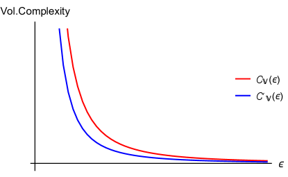
Figure 1: Static frame complexity, $\mathcal{C}_{V}$ and stationary frame complexity, $\mathcal{C}^{\prime}_{V}$ as a function the UV cutoff scale $\epsilon$.

In conclusion, we notice that the volume complexity for the LST deformed with Lorentz violating and nonlocal couplings leads to the exact same kind of divergences which nonlocality by itself would have produced (quadratic and logarithmic divergences). The distinctive signature of Lorentz boost violation is that the coefficients of the quadratic and logarithmic divergences as well as the finite piece in complexity differ in the two frames related by a Lorentz boost.

4 Subregion volume complexity

The volume complexity computed in the last section was unable to capture the distinguishing signatures of lorentz violation form nonlocality as far as the type of UV divergences appearing was concerned. In the hope that the subregion complexity might have something more to tell us about the differences between signatures of nonlocality and Lorentz violation, in this section we explore the features of subregion volume complexity for a boundary subregion of size $L$. To this end we have to focus our attention to the portion of the maximal volume slice which is contained within the Ryu-Takayanagi (RT) surface (curve) homologous to the aforementioned boundary spacelike interval (of size $L$) following the prescription of Alishahiha:2015rta .

First we briefly review the construction of the the RT surface in the dimensionally reduced $2+1$-d bulk gravity background, which is a codimension 2 surface in the bulk, homologous to the boundary subregion. The volume functional on a codimension-2 slice (in this case a curve) is obtained by looking at the constant time section of the $U=U(x)$ surface.

$$\begin{split}ds^{2}&=\left(kl_{s}^{2}{U^{\prime 2}\over U^{2}}+h(U)(1-f(U)(\epsilon_{+}+\epsilon_{-})^{2})\right)dx^{2},\end{split}$$ (48)

where, the prime denotes the derivative with respect to the parameter $x$ parameterizing the RT curve. In the string frame, this co-dimension-2 surface has the following volume functional, which in the present case turns out to be the length of the curve

$$\begin{split}\int dx\,\mathcal{L}(U(x),U^{\prime}(x),x)&={1\over U}\sqrt{kU^{\prime 2}l_{s}^{2}\left(k\lambda U^{2}+1\right)\left(kU^{2}\lambda^{\prime}+1\right)+kU^{4}\left(kU^{2}\mu+1\right)}.\end{split}$$ (49)

where, the primes over the quantities denotes their derivative with respect to $x$. Next, one has to minimize this string frame length functional to obtain the RT curve. However, instead follow the procedure of Chakraborty:2020udr and start by analyzing the integrals of motion. The condition that lagrangian is independent of time, gives us the first integral of motion

$$\begin{split}c_{1}&={\partial\mathcal{L}\over\partial t^{\prime}}\,~{}(=0),\end{split}$$ (50)

Since the lagrangian is cyclic in parameter $x$, the corresponding “hamiltonian” should be conserved:

$$\begin{split}c_{2}&=U^{\prime}{\partial\mathcal{L}\over\partial U^{\prime}}-\mathcal{L},\\ &={-kU^{3}\left(kU^{2}\mu+1\right)\over\sqrt{kU^{\prime 2}l_{s}^{2}\left(k\lambda U^{2}+1\right)\left(kU^{2}\lambda^{\prime}+1\right)+kU^{4}\left(kU^{2}\mu+1\right)}},\\ &=-\sqrt{k}U_{0}\sqrt{kU_{0}^{2}\mu+1},\end{split}$$ (51)

$c_{2}$ being a constant, we have used the boundary conditions at $x=0$ to evaluate $c_{2}$, i.e. $U(0)=U_{0}$ and $U^{\prime}(0)=0$ to evaluate it.

Solving for $U^{\prime}(x)$ and choosing the positive root,

$$\begin{split}U^{\prime}(x)&={U^{2}\sqrt{k\mu U^{2}+1}\sqrt{k\mu\left(U^{4}-U_{0}^{4}\right)+U^{2}-U_{0}^{2}}\over U_{0}l_{s}\sqrt{\left(k\lambda U^{2}+1\right)\left(k\lambda^{\prime}U^{2}+1\right)}\sqrt{k\mu U_{0}^{2}+1}}.\end{split}$$ (52)

To obtain the subregion size we integrate the above equation by specifying the appropriate limits of integration.

$$\int_{0}^{x}dx^{\prime} =\int_{U_{0}}^{U}{d\widetilde{U}\over\widetilde{U}^{\prime}(x)}.$$ (53)

After the integration limits had been specified, the subregion size is given as the function of the turning point $U_{0}$ by:

$$L =\int_{U_{0}}^{\infty}dU\,{dU\over U^{\prime}(x)}$$ (54)

If we choose to look at deep linear dilatonic region, ($k\lambda U^{2}>>1$) we obtain a simplification:

$$L ={\pi\sqrt{k\lambda\lambda^{\prime}}l_{s}\over 2\sqrt{\mu}}+O\left({1\over U_{0}^{2}}\right).$$ (55)

We can analytically solve for $L$ only perturbatively, but the characteristic features of subregion length in the linear dilaton region are immediately obvious. As we move $U_{0}$ closer to the boundary, $L$ asymptotes to a constant value:

$$L_{c} ={\pi\sqrt{k\lambda\lambda^{\prime}}l_{s}\over 2\sqrt{\mu}}.$$ (56)

This behaviour is typical of the theory having a Hagedorn phase transition as had already been alluded to before in the literature Chakraborty:2020udr in the context of the study of entanglement entropy using the $3+1$-d dual bulk background. (The critical length turns out to be the same).

We now perform some sanity checks by reproducing established results for different special cases from the general form equation (54) :

• AdS (Case $\lambda=\epsilon_{\pm}=0)$: The simplest of the all is the pure AdS geometry which has been the subject of an extensive study for which, the relation between the subregion length and the turning point is well known:

  $$\begin{split}L&={2l_{s}\over U_{0}}.\end{split}$$ (57)

• WAdS (Case $\lambda=\epsilon_{+}=0)$: The next case is when only the $J\overline{T}$ coupling is turned on. This case had also been thoroughly investigated and the gravity dual is warped AdS (WAdS) spacetime Azeyanagi:2012zd .

  $$\int_{0}^{L/2}dx^{{}^{\prime}} =\int_{U_{0}}^{{l_{s}\over\epsilon}}dU{U_{0}l_{s}\sqrt{1-kU_{0}^{2}\epsilon_{-}^{2}}\over U^{2}\sqrt{1-kU^{2}\epsilon_{-}^{2}}\sqrt{U^{2}-U_{0}^{2}+k\epsilon_{-}^{2}(-U^{4}+U_{0}^{4})}}$$ (58)

  $$\Rightarrow L ={2l_{s}\over U_{0}}+2kU_{0}l_{s}\epsilon_{-}^{2}\ln\left({{2l_{s}\over U_{0}\epsilon}}\right)+O(\epsilon_{-}^{4}).$$ (59)

  Upon turning off the coupling ($\epsilon_{-}\to 0$), one simply recovers the pure AdS result.

• $\mathcal{M}_{3}$ (Case $\epsilon_{+}=\epsilon_{-}=0)$: When only $T\overline{T}$ coupling is turned on,

  $$\begin{split}\int_{0}^{L/2}dx^{\prime}&=\int_{U_{0}}^{l_{s}/\epsilon}dU{U_{0}l_{s}\sqrt{k\lambda U^{2}+1}\sqrt{k\lambda U_{0}^{2}+1}\over U^{2}\sqrt{\left(U^{2}-U_{0}^{2}\right)\left(k\lambda\left(U^{2}+U_{0}^{2}\right)+1\right)}},\\ L&={1\over 2}\pi\sqrt{k\lambda}l_{s}+O\left({1\over U_{0}^{2}}\right),\end{split}$$ (60)

  we recover the result already encountered earlier in Chakraborty:2018kpr .

  Alternatively, treating coupling as the perturbation parameter,

  $$\begin{split}L&={2l_{s}\over U_{0}}+k^{2}\lambda^{2}U_{0}^{3}l_{s}\ln\left({2l_{s}\over U_{0}\epsilon}\right)+O(\lambda^{3}).\end{split}$$ (61)

  With $\lambda\to 0$, we again recover the AdS result.

Thus we have successfully reproduced the features of the RT curves for the special cases of the pure AdS, warped AdS and the $\mathcal{M}_{3}$ from our general formula relating the RT curve turning point and the subregion length (54). We will use this relation to obtain the expression for the subregion volume complexity next. This will be done numerically, since the analytic expressions can only be obtained perturbatively. Since we are not interested in perturbative answers, we will do this exactly but numerically. Just as we have done for the RT curve, before presenting the final results for the general case, we first perform sanity checks by studying various special cases where the effects of locality and Lorentz violation are removed and comparing those expressions to existing results in the literature obtained in the contexts where the boundary dual is a local CFT₂, instead of an LST₂.

4.1 Subregion volume (complexity) for $\lambda=\epsilon_{\pm}=0$: Poincare patch of AdS₃

The first check is the maximal volume corresponding to the subregion size ($\mathcal{V}(L)$) for the simplest of the cases - pure $AdS_{2+1}$. This can be evaluated analytically exactly. The induced metric on a codimension-$1$ submanifold of a constant time slice is

$$\begin{split}ds^{2}&={kl_{s}^{2}\over z^{2}}(dz^{2}+dx^{2}).\end{split}$$ (62)

Then subregion volume is,

$$\begin{split}\mathcal{V}(L)&=\int^{l_{s}/\epsilon}_{0}dz\int_{0}^{x(z)}dx^{\prime}e^{-2(\Phi(z)-\Phi_{\infty})}\sqrt{\gamma},\\ &=kl_{s}^{2}\left({L\over 2\epsilon}-{\pi\over 2}\right).\end{split}$$ (63)

The linear UV divergence is expected of any lorentz covariant local $CFT$ in one spatial dimension. This is a well known result Alishahiha:2015rta .

4.2 Subregion volume complexity $\epsilon_{\pm}=0$: $T\overline{T}$ deformation or $\mathcal{M}_{3}$

The next case we treat is a new result, although appropriately it belongs to the subject matter of the preceding work Chakraborty:2020fpt on pure $\mathcal{M}_{3}$ complexity. Since the subregion complexity calculation was omitted there, for the sake of completeness, we reproduce here the corresponding result for subregion complexity. In this case, the pullback of the ambient metric on codimension-$1$ surface bounded by the RT curve for the pure $\mathcal{M}_{3}$ case is:

$$\begin{split}ds^{2}&=kl_{s}^{2}{dU^{2}\over U^{2}}+h(U)dx^{2}.\end{split}$$ (64)

The volume corresponding to this subregion of the (maximal volume slice) as the function of the turning point $U_{0}$ is given by

$$\begin{split}\mathcal{V}&=\int_{U_{0}}^{l_{s}/\epsilon}dU\int_{0}^{x(U)}dx\,e^{-2(\Phi(U)-\Phi_{0})}\sqrt{\gamma},\\ &=kl_{s}\int_{U_{0}}^{l_{s}/\epsilon}dU\sqrt{1+k\lambda U^{2}}\int_{U_{0}}^{U}{d\widetilde{U}\over\widetilde{U}^{\prime}(x)}.\end{split}$$ (65)

We have to eliminate $U_{0}$ in favor of $L$ to express the maximal volume in terms of subregion length. However if we insist on analytical expression, then the inversion can only be achieved iteratively or perturbatively. In order to not compromise on precision, we instead perform the calculations numerically to illustrate the quantitative features of the subregion complexity.

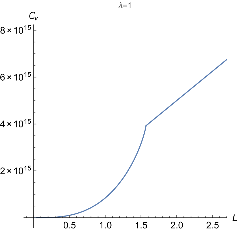
((a)) $\mathcal{C}_{V}\,vs\,L$  for  $\lambda=1$

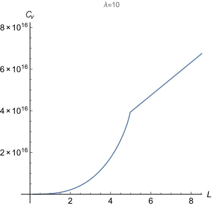
((b)) $\mathcal{C}_{V}\,vs\,L$  for  $\lambda=10$

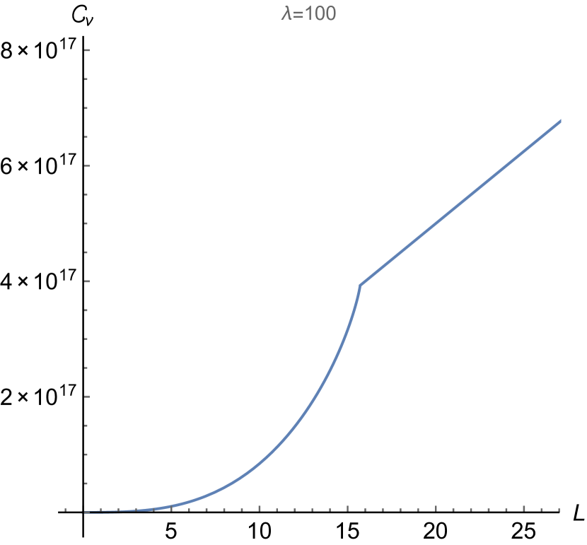
((c)) $\mathcal{C}_{V}\,vs\,L$  for  $\lambda=100$

Figure 2: Subregion volume complexity ($\mathcal{C}_{V}$) vs. subregion size ($L$) graphs for $T\overline{T}$ deformed CFT₂ (LST) for different values of the deformation parameter ($T\overline{T}$ coupling) $\lambda$ exhibiting Hagedorn phase transition. The critical suregion size at the transition point increases monotonically with $\lambda$.

In Fig. 2 we present the numerical plots demonstrating the dependence of complexity (modulo the factor of $8\pi G_{N}\sqrt{k}l_{s}$) on the subregion length $L$ for three different values (differing orders of magnitude) of $\lambda$, the $T\overline{T}$ deformation coupling parameter. All plots display the following universal traits

• The subregion volume complexity is a monotonically increasing function of the subregion size.

• The subregion volume complexity undergoes a sharpe (phase) transition as the subregion size is increased beyond a certain critical size as depicted by the presence of a kink in each of the plots.

• Once the subregion size is larger than the critical subregion (kink), the subregion volume complexity grows linearly with subregion size. This is characteristic of the AdS geometry as pointed out in the previous subsection 4.1. The RT curve extends deep into bulk where the geometry is close to AdS₃.

• The parabolic portion of the curve, for subregion size (length) is less than the critical length, pertains to the linear dilaton region because that is where the subregion size slowly approaches to a constant value $L_{c}$ regardless of the position of the turning point $U_{0}$ of the RT curve. The RT curve here remains stuck mostly in the deep UV region i.e. near the boundary.

The linear growth of the complexity with the subregion size when the subregion size is larger then the Hagedorn scale (see next section for more details) is plausible because in this situation the LST behaves more like a local CFT and the number of degrees of freedom in the Lorentz covariant local theory can be thought of as uniformly distributed along the boundary subregion. The kink signifies the termination of the linear dilaton geometry and bulk being subsequently taken over by the AdS geometry. It will turn out that same universal features will emerge when we introduce Lorentz violating effects in the system i.e. when the couplings $\epsilon_{\pm}$ are nonzero. In order to avoid repetition, we will leave further quantitative discussion to the next section where we tackle the case when Lorentz violating effects are turned on.

4.3 Subregion volume complexity for nonzero $\lambda,\epsilon_{\pm}$: $T\overline{T}$, $J\overline{T}$ and $\overline{J}T$ LST

Armed with the hints and insights from the previous sections for the various subcases (i.e. pure $AdS$ and $\mathcal{M}_{3}$), we are now ready to tackle the most general case with both the locality violating, and Lorentz violating couplings turned on and obtain the general characteristics for the subregion volume complexity. As was done in the previous section, we first record the pullback of the ambient metric on codimension two maximal volume surface, namely the constant $t$ surface, bounded by RT curve for the general case of the nonlocal as well as both of the Lorentz violating couplings turned on:

$$ds^{2}=kl_{s}^{2}{dU^{2}\over U^{2}}+h(U)(1-f(U)(\epsilon_{+}+\epsilon_{-})^{2})dx^{2}.$$ (66)

The maximal volume arising from the above geometry is given by:

$$\begin{split}\mathcal{V}&=\int_{U_{0}}^{l_{s}/\epsilon}dU\int_{0}^{x(U)}dxe^{-2(\Phi(U)-\Phi_{0})}\sqrt{\gamma},\\ &=kl_{s}\int_{U_{0}}^{l_{s}/\epsilon}dU\sqrt{1+k\mu U^{2}}\int_{U_{0}}^{U}{d\widetilde{U}\over\widetilde{U^{\prime}}(x)}.\end{split}$$ (67)

For the reasons alluded to earlier in the previous subsection, we again opt for a numerical approach to uncover the features of subregion complexity. The corresponding plots for $\mathcal{V}\,\,vs\,\,L$ (note that modulo the factor of $8\pi G_{N}\sqrt{k}l_{s}$, the complexity $\mathcal{C}_{V}$ and maximal slice volume $\mathcal{V}$ are the same) for various values of the Lorentz violating couplings against the fixed value of $\lambda=170$, are appended below in Fig. 3. In all the plots we notice some features which are in common with the $\mathcal{M}_{3}$ ($T\overline{T}$ deformation) set up, namely

• The subregion volume complexity is a monotonically increasing function of the subregion size

• The subregion complexity undergoes a phase transition as the subregion size is varied. For small subregions, we encounter a parabolic growth up to a kink at some critical subregion length, followed by the linear growth which is characteristic of dual AdS geometry in the deep IR. The parabolic region of the curve corresponds to the UV region i.e. linear dilaton geometry because that is where, the subregion length slowly approaches zero.

• For fixed $\lambda$ (i.e. nonlocality scale held fixed), the critical subregion size at the phase transition point in the plots increases (shifts rightwards) as the Lorentz-violating coupling $\epsilon_{+}$ ($\epsilon_{-}$) is increased. Interestingly the critical subregion size changes (increases) even if just one of the couplings $\epsilon_{+}$ is made nonzero. We will keep this in mind when we are looking at the static frame complexity where it will turn out that the critical subregion size is a function of the product $\epsilon_{+}\epsilon_{-}$.

In order to facilitate comparisons, its convenient to scale all the diagrams in a single plot by plotting the logarithms of complexity (modulo the factor of $8\pi G_{N}\sqrt{k}l_{s}$) and the subregion size $L$. From the graphs, one can directly appreciate the appearance of the transition point $L_{c}$ where the complexity characteristics transitions sharply from parabolic to the AdS like linear dependence. A phase transition in the holographic entanglement entropy as a function of subregion size for this same system has been shown in Chakraborty:2020udr . However, what is interesting is that, complexity not only undergoes an analogous phase transition, but that the subregion complexity phase transition occurs at the exact same critical subregion length as that of the entanglement entropy phase transition, as evident from table 1 displaying the numerical value of the critical length extracted from the plots and the theoretical expression for the critical subregion length for entanglement entropy (refer to Eq. (56)).

((a)) $\lambda=170,\epsilon_{\pm}=0$

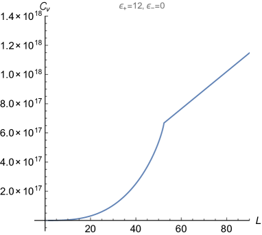
((b)) $\lambda=170$, $\epsilon_{+}=12,\epsilon_{-}=0$

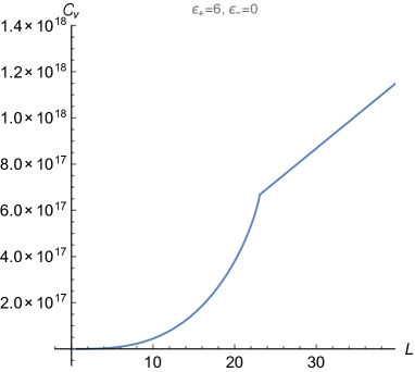
((c)) $\lambda=170$, $\epsilon_{+}=6,\epsilon_{-}=0$

((d)) $\lambda=170$, $\epsilon_{+}=7,\epsilon_{-}=6$

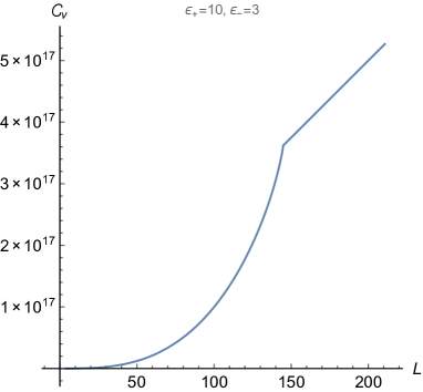
((e)) $\lambda=170$, $\epsilon_{+}=10,\epsilon_{-}=3$

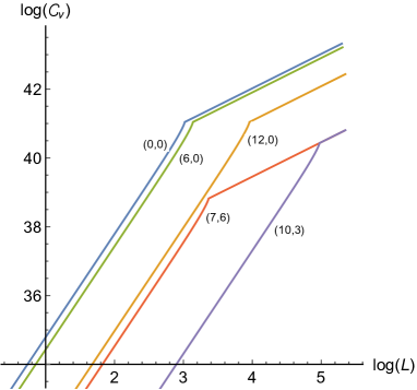
((f)) $\ln\mathcal{C}_{V}$ vs. $\ln L$  for $\lambda=170$

Figure 3: Subregion volume complexity ($\mathcal{C}_{V}$) vs. subregion size ($L$) graphs for $T\overline{T}$, $J\overline{T}$ & $\overline{J}T$ deformed CFT₂ (LST) for fixed values of the deformation parameter ($T\overline{T}$ coupling) $\lambda=170$ exhibiting Hagedorn phase transition. The last plot is a log-log graph clearly displaying the scaling exponents (slopes).

Critical subregion size for complexity for $\lambda=170$
Lorentz violating couplings ($\epsilon_{+}$,$\epsilon_{-}$)	Entanglement entropy transition point length $L_{c}$ (in units of AdS radius)	Subregion complexity transition point from graphs (in units of AdS radius)
(0,0)	20.48	20.47
(6,0)	23.06	23.05
(12,0)	52.37	52.33
(7,6)	28.96	28.94
(10,3)	144.82	144.9
(13,0)	267.03	266.84

Table 1: Table comparing the critical subregion size for phase transition in Entanglement entropy from theory and the critical subregion size for subregion volume complexity extracted from the plots

This fact that the subregion complexity undergoes a phase transition for the exact same the transition point (critical region size) as entanglement entropy, lends credence to the claim that complexity is a very effective physical observable (perhaps more useful that entanglement entropy) capable of detecting phase transitions (in the present case the Hagedorn phase transition) which perhaps cannot always be captured by usual field theory probes such as correlation functions of local operators.

4.4 Subregion volume complexity in static frame

Lorentz violating effects are our principal object of interest in this paper and in particular for the system under study i.e. LST our aim is to disentangle the effects of Lorentz violating from nonlocality. One way to perhaps isolate the characteristics of complexity corresponding to Lorentz violating effects in field theories is to examine complexity in different inequivalent Lorentz (boosted) frames. With such hope in this section we compute subregion complexity in a boosted frame (static frame) Eq. (32). To determine the RT curve we will first need the pullback ($\gamma_{ab}$) of the static metric on the one dimensional prospective RT curve is

$$ds_{\gamma}^{2}=\left(kl_{s}^{2}{U^{\prime 2}\over U^{2}}+f(U)\right)dX^{2}.$$ (68)

The length functional for this curve, parameterized as $U=U(X)$, in the string frame is given by

$$\int dX\,\,\mathcal{L}\left(U(X),U^{\prime}(X),X\right) =\int dXe^{-2(\Phi-\Phi_{0})}\sqrt{\gamma}=\int dX{kU^{2}\over\sqrt{f(U)h(U)}}\sqrt{kl_{s}^{2}{U^{\prime 2}\over U^{2}}+f(U)}.$$ (69)

Employing the same set of steps employed in the previous section we first compute the integrals of motion.

$$C_{2} =U^{\prime}{\partial\mathcal{L}\over\partial U^{\prime}}-\mathcal{L}=-{kU^{3}\sqrt{f(U)}\over\sqrt{h(U)}\sqrt{U^{2}f(U)+kU^{\prime 2}l_{s}^{2}}}=-{kU^{3}\sqrt{kU^{2}\lambda^{\prime}+1}\over\sqrt{kU^{\prime 2}l_{s}^{2}\left(k\lambda U^{2}+1\right)+kU^{4}}}$$ (70)

Integrals of motion after applying boundary conditions $U(0))=U_{0}~{}\text{and}~{}U^{\prime}(0)=0$ at the turning point to the above equation is

$$C_{2} =-\sqrt{k}U_{0}\sqrt{kU_{0}^{2}\lambda^{\prime}+1}.$$ (71)

Equating and solving for $U^{\prime}(X)$ gives

$$U^{\prime} ={U\sqrt{f(U)}\sqrt{U^{4}h\left(U_{0}\right)-U_{0}^{4}h(U)}\over\sqrt{k}U_{0}^{2}\sqrt{h(U)}l_{s}}$$ (72)

Inverting this, the subregion size can be expressed in terms of the turning point $U_{0}$ as

$$L=2\int_{0}^{L/2}dX=2\int_{U_{0}}^{\infty}{dU\over U^{\prime}}=2\sqrt{k}U_{0}^{2}l_{s}\int_{U_{0}}^{\infty}{\sqrt{h(U)}\over U\sqrt{f(U)}\sqrt{U^{4}h\left(U_{0}\right)-U_{0}^{4}h(U)}}$$ (73)

In the linear dilaton region, $(kU^{2}>>1)$, one can perturbatively solve the above equation to obtain

$$L ={1\over 2}\pi\sqrt{k\lambda}l_{s}+O\left(1/U_{0}^{2}\right)$$ (74)

This limiting value of $L$ in the static frame, named $L^{\prime}_{c}$ gives critical length of the subregion at the point of Hagedorn phase transition

$$L^{\prime}_{c}={1\over 2}\pi\sqrt{k\lambda}l_{s}$$ (75)

This is the critical subregion size where entanglement entropy (RT curve) undergoes the Hagedorn phase transition in the static frame. An important thing to note here that despite the Lorentz violating couplings, $\epsilon_{\pm}$, being turned on this leading order expression is independent of $\epsilon_{\pm}$, and instead depends just on the nonlocality parameter $\lambda$. The issue of whether this is true to all orders will be settled After determining the RT curve, now we determine the subregion complexity as the string frame area of the co-dimension one maximal area spacelike surface bound from the inside by the RT curve. The (pullback) metric on the maximal area (spacelike) hypersurface is:

$$\begin{split}ds^{2}&=kl_{s}^{2}{dU^{2}\over U^{2}}+f(U)dX^{2}.\end{split}$$ (76)

Thus the maximal volume arising from the above hypersurface bounded between the RT curve and the boundary is:

$$\mathcal{V} =\int_{U_{0}}^{l_{s}/\epsilon}dU\int_{0}^{X(U)}d\widetilde{X}e^{-2(\Phi(U)-\Phi_{\infty})}\sqrt{\gamma}=kl_{s}\int_{U_{0}}^{l_{s}/\epsilon}dU\sqrt{1+kU^{2}\lambda^{\prime}}\int_{U_{0}}^{U}{d\widetilde{U}\over\widetilde{U}^{\prime}}$$ (77)

We again opt for exact but numerical means in computing the subregion volume (complexity) instead of an analytic but perturbative (approximate) approach. The plots for subregion complexity vs. subregion size for various representative values of the Lorentz violating couplings $\epsilon_{\pm}$ and a fixed value the $T\overline{T}$ coupling $\lambda=170$ are displayed in figure (4).

((a)) $\lambda=170,\epsilon_{\pm}=0$

((b)) $\lambda=170$, $\epsilon_{+}=6,\epsilon_{-}=0$

((c)) $\lambda=170$, $\epsilon_{+}=12,\epsilon_{-}=0$

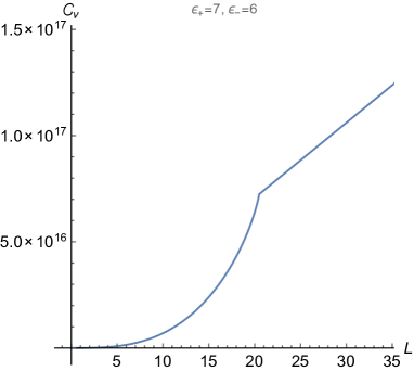
((d)) $\lambda=170$, $\epsilon_{+}=7,\epsilon_{-}=6$

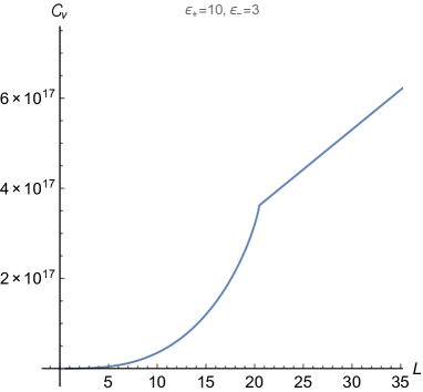
((e)) $\lambda=170$, $\epsilon_{+}=10,\epsilon_{-}=3$

((f)) $\ln\mathcal{C}_{V}$ vs. $\ln L$  for $\lambda=170$

Figure 4: Static frame subregion volume complexity ($\mathcal{C}_{V}$) vs. subregion size ($L$) graphs for $T\overline{T}$, $J\overline{T}$ & $\overline{J}T$ deformed CFT₂ (LST) for fixed $\lambda=170$ exhibiting Hagedorn phase transition. The last plot is a log-log graph clearly displaying the scaling exponents (slopes).

Here we list the salient features of these plots:

• Subregion volume complexity is a monotonically increasing function of the subregion size and it undergoes a phase transition as the subregion size is varied (just like subregion complexity in the stationary frame) beyond a certain critical length, which turns out to be $L^{\prime}_{c}$ of Eq. (75), i.e. the same critical subregion size at which entanglement entropy undergoes a phase transition (refer to table 2 ).

• For subregion size less than the critical size, $L^{\prime}_{c}$, complexity grows quadratically with subregion size while for subregion sizes greater than $L^{\prime}_{c}$, complexity grows linearly as evident from the log-log plot. The physics of this is the same as in that of the stationary frame - for small subregion sizes the RT curve is confined to the near boundary linear dilaton region, i.e. the deep UV regime of the boundary theor which is a nonlocal theory (LST on scales comparable to the string length scale), while for large subregion sizes the RT curve is well inside the bulk where the geometry is AdS, i.e. the deep IR regime of the boundary theory - LST on length scales far larger than the string scale and hence can be regarded as local CFT.

• Unlike in the stationary frame, in the static the critical subregion size at the transition point, extracted from the location of the kinks in the plots, does not change as the Lorentz violating couplings $\epsilon_{\pm}$ are varied while keeping the nonlocality scale $\lambda$ fixed. Refer to the table This strongly hints that perhaps the static frame complexity is a probe which is better suited to isolate or extract the effects of nonlocality while the complexity in the stationary frame manifests a mixed characteristic of both nonlocality and Lorentz violation.

• When either one or both of Lorentz violating couplings $\epsilon_{\pm}$ vanish, their graphs overlap to overlap. This is potentially due to the fact that the static frame subregion complexity becomes effectively the function of $\lambda^{\prime}=\lambda-4\epsilon_{+}\epsilon_{-}$, so that it is insensitive to distinguish between the various values of $\lambda^{\prime}$ for vanishing value of the product $\epsilon_{+}\epsilon_{-}$. So the characteristic signatures of Lorentz violation in the divergence structure is the one which is accompanied by the coefficient $\epsilon_{+}\epsilon_{-}$.

Location of the critical length $L^{\prime}_{c}$ for $\lambda=170$
Lorentz violating couplings ($\epsilon_{+}$,$\epsilon_{-}$)	Critical suregion size for entanglement entropy (EE) $L^{\prime}_{c}$ computed from Eq. (75)	Critical subregion size for subregion complexity in static frame extracted from $\mathcal{C}_{V}$-$L$ graphs Fig. 4
(0,0)	20.48	20.47
(6,0)	20.48	20.48
(12,0)	20.48	20.49
(7,6)	20.48	20.48
(10,3)	20.48	20.48
(13,0)	20.48	20.48

Table 2: Table comparing the critical subregion size for phase transition in Entanglement entropy from theory and the critical subregion size for subregion volume complexity extracted from the plots in the static Lorentz frame

As before, in the case of stationary frame subregion complexity, here we find it instructive to supply the table listing the critical subregion size from the plots for various cases of Loerntz violating couplings at a fixed $\lambda$ and compare it with the perturbatively calculated analytical estimate Eq. (75). It is evident form table 2 subregion volume complexity displays a phase transition at the exact same critical subregion size as that of entanglement entropy in the static frame. Thus, we can echo the same message from the end of the previous section regarding the utility of complexity as a physical probe for detecting phase transitions (perhaps even in those circumstances where other probes such as correlators of local operators might fail). However, unfortunately as long as $\lambda$ remains nonzero it appears one cannot isolate the effects of Lorentz violation from nonlocality in this system (LST) in this static frame. In fact, to the contrary, what we have seen in this exercise is that even if $\epsilon_{\pm}$ are not both zero, but if the product $\epsilon_{+}\epsilon_{-}$ vanishes, then the subregion complexity phase transition point is a pure function of the the nonlocality scale $\lambda$ i.e. in this boosted frame, the phase transition is independent of the Lorentz violating effects.

5 Holographic volume complexity of null WAdS₃

In this section we consider a special limit in the parameter space of the irrelevant couplings of the LST, for which the bulk dual is the null Warped AdS geometry, which is smoothly realised by sending $\lambda\rightarrow 0$ and one of the Lorentz violating coupling (say $\epsilon_{-}$) to zero. In this limit, the (stationary frame) bulk metric Eq. (17) becomes,

$$ds^{2}=kl_{s}^{2}{dU^{2}\over U^{2}}-h(U)\left(1+f(U)\epsilon_{-}^{2}\right)\,dt^{2}+2h(U)\,f(U)\,\epsilon_{-}^{2}\,dt\,dx+h(U)\left(1-f(U)\,\epsilon_{-}^{2}\right)dx^{2}$$ (78)

The Lorentz parameter $\epsilon_{-}$ can be identified with the warping parameter $\epsilon_{-}$. The boundary theory in this case is a warped CFT Detournay:2012pc ; Hofman:2014loa , a highly nonlocal Lorentz violating field theory with the CFT symmetry algebra now reduced to a semidirect product of Virasoro (left) and a $U(1)$ Kac-Moody algebra (right). In particular, for the null warped WAdS₃, the dual warped CFT is not UV complete, beyond a certain critical energy (deep UV) the theory is nonunitary since the energy spectrum is complex Chakraborty:2020xyz . Although correlation functions are hard compute in this warped CFT, we demonstrate that this feature (UV incompleteness) easily captured by complexity.

5.1 Volume Complexity

The maximal volume spacelike slice does not need to be worked out afresh as it can treated as a special case of the stationary frame metric of the generic $T\overline{T}$, $J\overline{T}$-$\overline{J}T$ deformed bulk geometry. However this limit could be singular so instead of indirectly evaluating the volume (complexity) by taking the naive $\lambda,\epsilon_{+}\rightarrow 0$ limit of the maximal volume expression of the string frame (40) (or complexity (41)) we compute the integral directly,

$$\begin{split}V_{\Sigma}(T)&=L_{x}kl_{s}\int dU\sqrt{1-\epsilon_{-}^{2}kU^{2}}={L_{x}kl_{s}^{2}\over 2\epsilon}\sqrt{1-{k\epsilon_{-}^{2}l_{s}^{2}\over\epsilon^{2}}}+{\sqrt{k}l_{s}L_{x}\over 2\epsilon_{-}}\sin^{-1}\left({\sqrt{k}\epsilon_{+}l_{s}\over\epsilon}\right)\\ \Rightarrow\mathcal{C}_{V}&={L_{x}\sqrt{k}l_{s}\over 2G_{N}\epsilon}\sqrt{1-{k\epsilon_{-}^{2}l_{s}^{2}\over\epsilon^{2}}}+{L_{x}\over 2\epsilon_{-}G_{N}}\sin^{-1}\left({\sqrt{k}\epsilon_{-}l_{s}\over\epsilon}\right)\end{split}$$ (79)

Here, we see that the resultant complexity, unlike for the generic case, (27), fails to remain real unless $\epsilon>\sqrt{k}l_{s}\,\epsilon_{-}$. Thus the UV cut off cannot be made arbitrarily small. This validates our faith that complexity successfully captures the UV incompleteness of the warped CFT dual to null warped AdS₃. In the limit of a small warping parameter $\epsilon_{-}$ (to be precise expanding in $\epsilon_{-}\sqrt{k}l_{s}/\epsilon$), the leading term is linearly divergent,

$$\mathcal{C}_{V}\sim{L_{x}\,\sqrt{k}\,l_{s}\over G_{N}\,\epsilon}-{L_{x}\,\left(\sqrt{k}l_{s}\right)^{3}\epsilon_{-}^{2}\over 6G_{N}\,\epsilon^{3}}$$ (80)

i.e. like a local field theory in one space dimensions (or pure AdS bulk)! Again this is a reflection that the UV regime (near boundary region) where the nonlocality effects kicks in is excluded from consideration. The complexity characteristics of Warped CFT in general from both the holographic and field theory methods has been taken up in greater detail in a separate paper Bhattacharyya:2022ren .

5.2 Subregion volume complexity for null WAdS₃

Finally we work out the subregion volume complexity for the interesting special case of null warped AdS₃. In this case first the result will be obtained analytically in the approximation of small warping $\epsilon_{-}$ to underscore the fact that subregion complexity is a better probe of nonlocality in this example compared to other probes such as subregion entanglement entropy. Then the exact result will be presented by evaluating the subregion complexity integral numerically without any approximations. First, recall that In this case, the turning point of the RT surface (curve) in terms of the subregion size is already worked out by inverting (58),

$$U_{0}={2l_{s}\over L}+{8kl_{s}^{3}\epsilon_{-}^{2}\over L^{3}}\ln\left({L\over\epsilon}\right)+O[\epsilon_{-}^{4}]$$ (81)

In terms of the turning point, the subregion volume complexity calculation of null WAdS₃ is given by the nested integral,

$$C_{V} ={\sqrt{k}l_{s}\over 8\pi G}\int_{U_{0}}^{{l_{s}\over\epsilon}}dU\sqrt{1-kU^{2}\epsilon_{-}^{2}}\int_{U_{0}}^{U}d\widetilde{U}{U_{0}\sqrt{1-kU_{0}^{2}\epsilon_{-}^{2}}\over\widetilde{U}^{2}\sqrt{1-k\widetilde{U}^{2}\epsilon_{-}^{2}}\sqrt{\widetilde{U}^{2}-U_{0}^{2}+k\epsilon_{-}^{2}(-\widetilde{U}^{4}+U_{0}^{4})}}$$ (82)

$$={\sqrt{k}l_{s}\over 8\pi G}\int_{U_{0}}^{{l_{s}\over\epsilon}}\bigg{[}{\sqrt{U^{2}-V^{2}}\over UV}-\bigg{(}{kU\sqrt{U^{2}-U_{0}^{2}}\over 2U_{0}}-kU_{0}\ln{\bigg{(}{U+\sqrt{U^{2}-U_{0}^{2}}\over U_{0}}\bigg{)}}\bigg{)}\epsilon_{-}^{2}+O\left(\epsilon_{-}^{4}\right)\bigg{]}dU$$ (83)

$$={\sqrt{k}l_{s}\over 8\pi G}\bigg{[}\bigg{(}1+{4kl_{s}^{2}\over L^{2}}\epsilon_{-}^{2}\bigg{)}{L\over 2\epsilon}-{kl_{s}^{2}L\over 12\epsilon^{3}}\epsilon_{-}^{2}-{\pi\over 2}O\left(\epsilon_{-}^{4}\right)\bigg{]}$$ (84)

In order to get eqn (84), we have expanded the integrands in equation (82) in a Taylor series with respect to $\epsilon_{-}$. In the above expression of $C_{V}$, we can clearly see that if we take the warping factor to be zero, equation (84) reproduces the subregion complexity for the pure $AdS_{3}$. For, pure $AdS_{3}$, we recover the expression for subregion volume complexity Alishahiha:2015rta ,

$$C_{V}={\sqrt{k}l_{s}\over 8\pi G}\bigg{[}{L\over 2\epsilon}-{\pi\over 2}\bigg{]}$$ (85)

Another very important feature of this result (84) is that the subregion $C_{V}$ (the divergence structure) reflects the nonlocal nature of the dual warped conformal field theory unlike the holographic entanglement entropy in the appendix D. While we are using a string background with all NS-NS sector fields turned on in the bulk, this local theory like divergence structure (linear divergence) of EE for Warped AdS₃ has been reported using other holographic backgrounds where the bulk theory is either topologically massive gravity (TMG) Anninos:2013nja ; Castro:2015csg or new massive gravity (NMG) Basanisi:2016hsh . Thus in this example, we see that subregion complexity is a more sensitive or refined probe of nonlocality and Lorentz violation compared to entanglement entropy.
Next we present the plot of Subregion $C_{V}$ as a function of $L$ in the figure below obtained by direct numerical evaluation of (82).

The value of $\epsilon_{-}=10^{-6}$ is used for this plot because from Eq. (79), it is clear that the value of $\epsilon_{-}$ has to be smaller than the value of $\epsilon$. Also note that here, the $y$-axis is actually complexity scaled by the universal constant $8\pi G_{N}$. We summarize the salient features of this plot

• Subregion complexity monotonically increases as a function of the subregion size.

• Unlike in the case of generic nonvanishing $\lambda,\epsilon_{+}$ the subregion complexity does not undergo any phase transition.

• The effect of nonlocality or Lorentz violation is very small in general and only prominent when the subregion is orders of magnitude smaller than the AdS radius. For larger generic subregion sizes the WAdS subregion $\mathcal{C}_{V}$ coincides with that for pure AdS₃ (this part needs to be discussed later.)

• Sensible plots are only obtained when the cut off $\epsilon>\epsilon_{-}$. This is again a reflection of the fact that the dual boundary theory is not a UV complete theory, it is best thought of as an effective theory with the spectrum truncated at high energies.

One might ask whether one can switch to the static frame and evaluate the complexity of LST dual to null warped AdS₃ in the that frame just like it was done in the case of generic $J\overline{T},\overline{J}T$ couplings to demonstrate/check for boost symmetry violation. However in this regard we would like to point out that boost transformation ((31)) is singular in the null warped AdS₃ limit, i.e. when $\epsilon_{+}\rightarrow 0$. Thus neither such a boost transformation and by extension, nor does a static frame exist for null warped AdS₃. In this special point of the parameter space, we will have to be content with the volume complexity, subregion volume complexity and action complexity in the stationary coordinate system exclusively.

6 Action complexity

In this section we compute the action complexity, $C_{\mathcal{A}}$, for the LST obtained by $T\overline{T},J\overline{T},\overline{J}T$ deformation of a CFT₂ using the holographic dual metric, dilaton and Kalb-Ramond background. Action complexity is an alternative prescription of holographically evaluating the dual boundary theory complexity which offers distinct advantages over volume complexity in that (A) no arbitrary length scales appearing in its definition, just the fundamental constants $\hbar$ and $G_{N}$, and (B) one does need to solve a variational problem which can be challenging exercise in general for Lorentzian signature spacetimes. Instead one just performs (action) integrals over the WdW patch. The WdW patch is defined as the union of all spacelike hypersurfaces in the bulk anchored at a fixed timeslice on the boundary:

$$C_{\mathcal{A}}={S_{WdW}\over\pi\hbar}~{}.$$ (87)

The Penrose diagram of the dual bulk geometry (suppressing the transverse boundary direction) is identical to that of the $\mathcal{M}_{3}$ spacetime, presented in our previous work Chakraborty:2020fpt . For completeness, we reproduce the Penrose diagram here with the WdW patch displayed in pink

Figure 6: Penrose diagram of the dual bulk geometry with the Wheeler-deWitt (WdW) patch shaded in pink for the boundary time $T$. The brown curves are timelike surfaces which can be continuously deformed into the null boundaries of the WdW patch by means of a regulator parameter.

The bulk action in the string frame is:

$$\begin{split}S&={1\over 16\pi G_{N}}\int_{M}d^{d+1}X\sqrt{-g}e^{-2(\Phi-\Phi_{0})}\left(R+4g^{\mu\nu}\partial_{\mu}\Phi\partial_{\nu}\Phi-{H^{2}\over 12}-4\Lambda\right)\\ &\hskip 72.26999pt+{1\over 8\pi\,G_{N}}\int_{\sum\partial M}\sqrt{\gamma}\,\left(\cdots\right)+{1\over 8\pi\,G_{N}}\int_{\cap\partial M}\sqrt{h}\,(\cdots)~{}.\end{split}$$ (88)

The $(\cdots)$’s represent the supplementary surface/boundary ($\cup\partial M$) terms and joint ($\cap\,\partial M$) terms necessary for the variation of the action to be well defined, as well as reparametrization invariant. Since (some) boundaries of the WdW patch are null, the usual GHY terms are not the suitable ones. The issue of determining the boundary terms for null boundaries was settled in Lehner:2016vdi . However, we will take an alternative prescription spelled out in Bolognesi:2018ion where the null boundaries of the WdW patch are first deformed into a single smooth timelike surface using a deformation parameter (regulator), and then we are free to use the usual GHY term. After working out the GHY term we remove the regulator and obtain the result for the null WdW boundary. This affords an enormous simplification as it eliminates the necessity to compute the joint terms (i.e. terms in the action from joints or edges along which two null surfaces intersect) as well as preserving diffeomorphism and reparametrization invariance of the GHY contribution from beginning to end. Our regularization reproduces the same results as the prescription of Lehner:2016vdi for the well known cases of pure AdS, AdS-Schwarzschild, AdS-RN etc. but the status of the equivalence of these two prescriptions for arbitrary generic geometries is yet unexplored. In general the issue of different regularization prescriptions is still being investigated e.g. for a comparison of the two regularizations introduced in Carmi:2016wjl , see Akhavan:2018wla ; Jafari:2019qns .

Just to remind the reader, that unlike for the $\mathcal{M}_{3}$ case, here one has to make a choice: one can either work with the full 4 dimensional bulk action, or one might dimensionally reduce (over the $y$-direction fiber) and work with an effective $3$ dimensional bulk action. While computing the entanglement entropy for this system, the authors of Chakraborty:2020udr found that the 4d and 3d results disagree and they opted to work with the full 4d bulk. Happily for us, it turns out that both 4d and 3d actions deliver identical results for complexity, provided one does not drop the total derivative terms in the dimensionally reduced action. Conventionally in the literature these total derivative terms are dropped since they do not contribute to the classical equations of motion. However while computing complexity these terms do contribute and one cannot discard them if the complexity before and after dimensional reduction has to match. In appendix Sec. B, the KK reduction is reviewed and the exact match between the 4D and 3D actions is carried out after retaining all total derivative terms in the dimensionally reduced (3D) action.

$$S_{(3D)} ={1\over 16\pi G_{N}}\int d^{3}x\sqrt{-g}~{}e^{-2\left(\Phi-\Phi_{0}\right)}\Big{(}R-\left(\partial\sigma\right)^{2}-2\,\Box\sigma-{1\over 4}e^{2\sigma}\mathcal{F}^{2}-4\Lambda$$

$$\hskip 199.16928pt+4g^{\mu\nu}\partial_{\mu}\Phi\partial_{\nu}\Phi+4g^{\mu\nu}\partial_{\mu}\Phi\partial_{\nu}\sigma$$

$$\hskip 256.0748pt-{1\over 12}\widetilde{H}^{2}-{1\over 4}e^{-2\sigma}\widetilde{F}^{2}\Big{)}.$$ (89)

It is evident that after dimensionally reducing to $3$ dimensions the KK scalar, $\sigma$ contributes to the action a term which has a second order derivative, namely $\Box\sigma$ (This is a total derivative term which is usually dropped). This will also to lead an extra contribution to the surface terms (GHY terms) in the string frame, apart from the usual GHY surface term arising from the metric. The full surface term contribution for the $2+1$-dimensional bulk in string frame is

$$S_{GHY}={1\over 8\pi G_{N}}\int d^{2}x\sqrt{-\gamma}\,e^{-2(\Phi-\Phi_{0})}\left(K+n^{\mu}\partial_{\mu}\sigma\right)~{}$$ (90)

For the derivation, the reader may refer to Appendix C. For the action complexity calculation, in the first order of business is to determine the WdW patch, i.e. the light cones emanating from the boundary timeslice. However, solving the WdW patch is very complicated in the stationary frame coordinates (17) where constant $t$ surfaces are not orthgonal to the vector $\partial/\partial t$. Life is much simpler in the static frame coordinates (32) as the constant $T$ surfaces are orthogonal to the time direction vector $\partial/\partial T$. So we perform the action complexity calculation exclusively in the static frame (32).

6.1 Volume (EH) pieces of the onshell action

In this section we present the volume piece contributions (“EH terms”) to the action complexity using the dimensionally reduced $2+1$-d background. As mentioned previously, the evaluation of the gravitational action (“EH terms”) in the string frame in $4$ dimensional and the dimensionally reduced $3$ dimensional backgrounds give identical results, for this equivalence, the reader is referred to the Sec.  B.2.
First we have to determine the WdW patch. As we have mentioned earlier, the calculation is most straightforward in the static coordinates $(T,X,U)$ because the lightcones are easy to determine. The Wheeler-deWitt patch (WdW) for the boundary time $T=T_{*}$ is bounded by the null rays

$$\,dt_{\pm} = \mp\sqrt{k}\,l_{s}\,{1\over U\sqrt{h(U)}}dU,$$ (91)

obeying boundary condition, $T(U\rightarrow\infty)=T_{*}$. The $T$-integrals in the volume terms (89) (Einstein-Hilbert plus matter type terms) can be readily done:

$$T_{+}(U)-T_{-}(U)=2\sqrt{k}\,l_{s}\,\int^{\infty}_{U}d\widetilde{U}{1\over\widetilde{U}\sqrt{h(\widetilde{U})}}~{}.$$ (92)

This integral is divergent and hence we will modify our WdW patch to begin at a UV-cutoff surface $U=l_{s}/\epsilon$ instead of spatial infinity:

$$T_{+}(U)-T_{-}(U)=2\sqrt{k}\,l_{s}\,\int^{l_{s}/\epsilon}_{U}d\widetilde{U}{1\over\widetilde{U}\sqrt{h(\widetilde{U})}}~{}.$$ (93)

Having determined the WdW patch, we list the various bulk action term contributions (89) along with their UV and IR limits are listed as follows.

The Ricci scalar sector term: These terms are from the $4$ dimensional Ricci scalar or equivalently in $3$ dimensions from the full KK reduced sector derived from the $4$ dimensional metric. For details the reader is referred to Sec. B.2.4.

$$\begin{split}S_{R}&\equiv{1\over 16\pi G_{N}}\int_{WdW}d^{3}x\sqrt{-g}~{}e^{-2(\Phi-\Phi_{0})}\left(R^{(3)}-2\left(\partial\sigma\right)^{2}-2\square\sigma-{1\over 4}e^{2\sigma}\mathcal{F}^{2}\right),\\ &={L_{x}k\over 8\pi G_{N}}\int_{0}^{l_{s}/\epsilon}dU\,U{\left(8\lambda^{\prime}kU^{2}-6\right)\over\left(\lambda^{\prime}kU^{2}+1\right)^{2}}\int^{l_{s}/\epsilon}_{U}dU^{\prime}{1\over U^{\prime}\sqrt{h(U^{\prime})}}~{}.\end{split}$$ (94)

The above integral can be performed analytically but the full expression is a bit cumbersome. In the deep UV (i.e. when $\epsilon/\beta_{H}\ll 1$), $S_{R}$ takes the following form

$$\begin{split}\lim_{\epsilon/\beta_{H}\ll 1}S_{R}=&-{cL_{x}\over 6\beta^{\prime}_{H}}(7+8\log 2)\log\left({\beta^{\prime}_{H}\over\pi\epsilon}\right)+{2cL_{x}\over 3\beta^{\prime}_{H}}\log^{2}\left({\beta^{\prime}_{H}\over\pi\epsilon}\right)\\ &\hskip 85.35826pt+{L_{x}c\over 18\beta^{\prime}_{H}}(\pi^{2}+24\log 2)+O\left(\left({\epsilon\over\beta^{\prime}_{H}}\right)^{2}\right)~{}.\end{split}$$

In the IR (i.e. when $\epsilon/\beta_{H}\gg 1$), $S_{R}$ takes the form

$$\lim_{\epsilon/\beta_{H}\gg 1}S_{R}=-{cL_{x}\over 4\pi\beta^{\prime}_{H}}{\beta^{\prime}_{H}\over\epsilon}+{7cL_{x}\over 288\pi^{3}\beta^{\prime}_{H}}\left({\beta^{\prime}_{H}\over\epsilon}\right)^{3}+O\left(\left({\beta^{\prime}_{H}\over\epsilon}\right)^{4}\right)~{}.$$ (95)

The dilaton kinetic term in the action: We refer the reader to Sec. B.2.2 for the details.

$$\begin{split}S_{\Phi}&\equiv{1\over 16\pi G_{N}}\int_{WdW}d^{3}x\,\sqrt{-g}\,e^{-2(\Phi-\Phi_{0})}4g^{\mu\nu}\partial_{\mu}\Phi\partial_{\nu}\Phi,\\ &={\lambda^{\prime 2}k^{3}L_{X}\over 2\pi G_{N}}\int_{0}^{{l_{s}\over\epsilon}}dU\>{U^{5}\over\left(1+\lambda^{\prime}\>kU^{2}\right)^{2}}\int_{U}^{{l_{s}\over\epsilon}}{dU^{\prime}\over U^{\prime}\sqrt{h(U^{\prime})}}.~{}\end{split}$$ (96)

In the UV regime, $S_{\Phi}$ takes the following form:

$$\begin{split}\lim_{\epsilon\ll\beta^{\prime}_{H}}S_{\Phi}={cL_{x}\over 24\pi^{2}\beta^{\prime}_{H}}\left({\beta^{\prime}_{H}\over\epsilon}\right)^{2}+\left(3+8\ln 2\right){cL_{x}\over 6\beta^{\prime}_{H}}\ln\left({\beta^{\prime}_{H}\over\pi\epsilon}\right)-{2cL_{x}\over 3\beta^{\prime}_{H}}\ln^{2}\left({\beta^{\prime}_{H}\over\pi\epsilon}\right)\\ +\left(3-2\pi^{2}-48\ln 2\right){cL_{x}\over 36\beta^{\prime}_{H}}+O\left({\epsilon\over\beta^{\prime}_{H}}\right)..\end{split}$$ (97)

One might be a bit alarmed at the appearance of the “log squared” divergences in the expressions (6.1) and (97), which did not arise in the volume complexity cases but as it will turns out, such log squared divergent contributions will cancel out among each other.
In the IR, $S_{\Phi}$ takes the form

$$\lim_{\epsilon/\beta_{H}\gg 1}S_{\Phi}=0+O\left(\beta_{H}^{5}/\epsilon^{5}\right)~{}.$$ (98)

The cosmological constant term in the action: The details are worked out in Sec. B.2.3. Here we present the main results starting from the $3$ dimensional action,

$$\begin{split}S_{\Lambda}&\equiv{1\over 16\pi G_{N}}\int d^{3}x\sqrt{-g}e^{-2\left(\Phi-\Phi_{0}\right)}\left(-4\Lambda\right),\\ &={L_{x}k\over 2\pi G_{N}}\int_{0}^{l_{s}/\epsilon}dU\,U\int^{l_{s}/\epsilon}_{U}dU^{\prime}{1\over U^{\prime}\sqrt{h(U^{\prime})}}~{}.\end{split}$$ (99)

In the UV, $S_{\Lambda}$ takes the following form

$$\lim_{\epsilon/\beta^{\prime}_{H}\ll 1}S_{\Lambda}={c\over 24\pi^{2}}{L_{x}\over\beta^{\prime}_{H}}\left({\beta^{\prime}_{H}\over\epsilon}\right)^{2}+{c\over 6}{L_{X}\over\beta^{\prime}_{H}}\ln\left({\text{$\beta^{\prime}_{H}$}\over\pi\epsilon}\right)+{c\over 12}{L_{x}\over\beta^{\prime}_{H}}+O\left({\epsilon\over\beta^{\prime}_{H}}\right)~{}.$$ (100)

In the IR, $S_{\Phi}$ takes the form

$$\lim_{\epsilon\gg\beta_{H}}I_{\Lambda}={cL_{x}\over 6\pi\epsilon}+{cL_{x}\over 144\pi^{3}\beta^{\prime}_{H}}\left({\beta^{\prime}_{H}\over\epsilon}\right)^{3}+O\left(\left({\beta^{\prime}_{H}\over\epsilon}\right)^{5}\right).$$ (101)

The Kalb-Ramond term in the action: Finally the spacetime volume type contribution from the Kalb-Ramond field in $4$ dimensions or the full Kalb-Ramond derived fields in $3$ dimensions after dimensional reduction (a Kalb-Ramond two-form field and a Kalb-Ramond one-form gauge field). The details including the matching before and after dimensional reduction are worked out in the appendix Sec. B.2.1. The main results starting with the action piece are presented here,

$$\begin{split}S_{H}&\equiv{1\over 16\pi G_{N}}\int\>d^{3}x\;\sqrt{-g}e^{-2(\Phi-\Phi_{0})}\left(-{1\over 12}\widetilde{H}^{2}-{1\over 4}e^{-2\sigma}\widetilde{F}^{2}\right),\\ &={L_{x}\over 4\pi G_{N}k}\int\,dU\,{h^{2}(U)\over U^{3}}\int_{U}^{{l_{s}\over\epsilon}}dU^{\prime}{1\over U^{\prime}\sqrt{h(U^{\prime})}}~{}.\end{split}$$ (102)

In the UV, $S_{H}$ takes the following form

$$\lim_{\epsilon/\beta_{H}\ll 1}S_{H}={cL_{x}\over 6\beta^{\prime}_{H}}\ln\left({\beta^{\prime}_{H}\over\pi\epsilon}\right)+O\left({\epsilon\over\beta^{\prime}_{H}}\right).$$ (103)

In the IR, $S_{H}$ takes the form

$$\lim_{\epsilon/\beta_{H}\gg 1}S_{H}={cL_{x}\over 12\pi\beta^{\prime}_{H}}\left({\beta^{\prime}_{H}\over\epsilon}\right)-{cL_{x}\over 288\pi^{3}\beta^{\prime}_{H}}\left({\beta^{\prime}_{H}\over\epsilon}\right)^{3}+O\left(\left({\beta^{\prime}_{H}\over\epsilon}\right)^{5}\right).$$ (104)

6.1.1 Action Contributions from the null boundaries of the WdW patch.

The WdW patch action receives surface contributions (GHY terms) from the boundaries of the $WdW$ patch. The Poincaré horizon and the two joint terms (intersection of the null boundaries of the WdW patch with the Poincaré horizon) make vanishing contributions. The only non trivial contribution comes from the two null boundaries of the WdW patch.
The null boundaries of the WdW patch are defined by

$$(T-T_{*})=\mp\sqrt{k}l_{s}A(U)~{};\quad\text{where }\ \ A(U)=\int_{l_{s}/\epsilon}^{U}{d\widetilde{U}\over\widetilde{U}\sqrt{h(\widetilde{U})}}~{}.$$ (105)

However, we will deform the pair of null surfaces to a single smooth timelike surface by introducing a dimensionless parameter, $\varepsilon$,

$${(T-T_{*})^{2}\over kl_{s}^{2}}-(1+\varepsilon)A^{2}(U)=0~{}.$$ (106)

Taking differentials of both sides leads to,

$$h(U)dT^{2}=(1+\varepsilon)kl_{s}^{2}{dU^{2}\over U^{2}}~{}.$$ (107)

Using (107), the induced metric on this timelike surface can be written as

$$ds^{2}=-\varepsilon kl_{s}^{2}{dU^{2}\over U^{2}}+h(U)(1-4\epsilon_{+}\epsilon_{-}f(U))dX^{2}~{}.$$ (108)

The negative sign in the first term clearly indicates that this is a timelike surface. The unit outward normals to the surface (106) are,

$$n^{T}={-(T-T_{*})\over\sqrt{(1+\varepsilon)^{2}A^{2}(U)-{(T-T_{*})^{2}\over kl_{s}^{2}}}}{1\over\sqrt{k}l_{s}\sqrt{h(U)}},\ \ \ n^{U}={-(1+\varepsilon)A(U)\over\sqrt{(1+\varepsilon)^{2}A^{2}(U)}-{(T-T_{*})^{2}\over kl_{s}^{2}}}{U\over\sqrt{k}l_{s}},\ \ \ n^{X}=0.$$ (109)

The trace of the extrinsic curvature,

$$\begin{split}K\equiv\nabla_{L}n^{L}=\partial_{L}n^{L}+\Gamma^{L}_{LM}n^{M}=\partial_{T}n^{T}+\partial_{U}n^{U}+\Gamma^{L}_{LU}n^{U}~{},\end{split}$$ (110)

takes the form

$$K = {1\over\sqrt{\varepsilon}\sqrt{k}l_{s}(1+kU^{2}\lambda)}+{1\over\sqrt{\varepsilon}\sqrt{k}l_{s}(1+kU^{2}\lambda^{{}^{\prime}})}~{}.$$ (111)

Thus the GHY term for this surface in the null limit ($\varepsilon\rightarrow 0$) is

$$\begin{split}S^{\partial WdW}_{GHY}&={1\over 8\pi G_{N}}\int_{\partial WdW}d^{2}x\,\sqrt{-\gamma}e^{-2\left(\Phi-\Phi_{0}\right)}\left(K+n^{\mu}\partial_{\mu}\sigma\right),\\ &=\lim_{\varepsilon\to 0}{L_{x}\sqrt{k}\over 4\pi G_{N}}\int_{0}^{l_{s}/\epsilon}{dU\over\sqrt{1+kU^{2}\lambda^{{}^{\prime}}}}~{},\\ &={cL_{x}\over 3\beta_{H}^{{}^{\prime}}}\ln\left(\sqrt{1+{\beta_{H}^{{}^{\prime}2}\over 4\pi^{2}\epsilon^{2}}}+{\beta_{H}^{{}^{\prime}}\over 2\pi\epsilon}\right)~{}.\end{split}$$

In the UV, $S^{\partial WdW}_{GHY}$ diverges as

$$\lim_{\epsilon/\beta_{H}\ll 1}S^{\partial WdW}_{GHY}={L_{x}c\over 3\beta_{H}^{{}^{\prime}}}\ln\left({\beta_{H}^{{}^{\prime}}\over\pi\epsilon}\right)+O\left(\epsilon/\beta_{H}^{{}^{\prime}}\right)~{}.$$ (112)

In the IR one can write

$$\lim_{\epsilon/\beta_{H}\gg 1}S^{\partial WdW}_{GHY}={L_{x}c\over 6\pi\beta_{H}^{{}^{\prime}}}\left({\beta_{H}^{{}^{\prime}}\over\epsilon}\right)-{L_{x}c\over 144\pi^{3}\beta_{H}^{{}^{\prime}}}\left({\beta_{H}^{{}^{\prime}}\over\epsilon}\right)^{3}+O\left(\beta_{H}^{{}^{\prime}4}/\epsilon^{4}\right)~{}.$$ (113)

6.2 Action Complexity

Gathering all the pieces, the full on-shell action over the WdW patch is obtained by summing over the contributions (94),(96),(99),(102), and (6.1.1). In the UV regime or the linear dilaton region (i.e. when $\epsilon/\beta_{H}\ll 1$), the action complexity (obtained by summing over the contributions (6.1),(97), (100),(103),and (112)) diverges as

$$C_{\mathcal{A}}={L_{x}c\over 3\pi^{2}\beta^{\prime}_{H}}\left[{{\beta^{\prime}_{H}}^{2}\over 2\pi\epsilon^{2}}-2\pi\log\left({\beta^{\prime}_{H}\over\pi\epsilon}\right)+\pi+O\left({\epsilon\over\beta^{\prime}_{H}}\right)\right].$$ (114)

Comparison this action complexity result with the (static frame) volume complexity expression (44) reveals that the leading divergence structure (i.e. the quadratic divergent term) and the constant term in both cases are identical. The subleading logarithmic divergences differ by a negative sign. In the IR (i.e. when $\epsilon/\beta^{\prime}_{H}\gg 1$) the action complexity takes the form

$$\lim_{\epsilon/\beta^{\prime}_{H}\gg 1}C_{\mathcal{A}}={cL_{x}\over 18\pi^{3}\beta^{\prime}_{H}}\left({\beta^{\prime}_{H}\over\epsilon}\right)^{2}+O\left({\beta^{\prime}_{H}}^{5}/\epsilon^{5}\right)~{}.$$ (115)

Thus in pure $AdS_{3}$ limit, i.e. $\beta^{\prime}_{H}=0$, the action complexity vanishes. This is in precise agreement with the analysis performed in Reynolds:2016rvl , a dimensional accident (there is a coefficient $C_{d}=d-2$ in the pure AdS_d+1 action complexity). Unlike the volume complexity, the action complexity decreases faster. A comparison between volume complexity and action complexity is presented in figure 7.

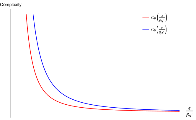
Figure 7: Comparison between $C_{V}$ and $C_{\mathcal{A}}$ at zero temperature. For large $\epsilon/\beta_{H}$, the action complexity decays much faster than volume complexity.

Thus overall, both the volume complexity and the action complexity diverges quadratically in the UV (i.e. when $\epsilon/\beta_{H}\to 0$). However, as $\epsilon/\beta_{H}$ increases, the action complexity decreases (much faster than volume complexity) monotonically eventually going to 0 in the deep IR. This discrepancy can be traced back to the boundary being $1+1$ dimensional, the action complexity has a coefficient $C_{d}=d-2$. But in general it is understood that complexity is arbitrary or ambiguous up to such numerical factors and in general dimensions the volume and action complexity divergences will match both in the UV and IR.

7 Action Complexity for null WAdS₃

We conclude this work by presenting the results for the action complexity of the null warped AdS₃ defined by the limit $\lambda=\epsilon_{+}=0$. We cannot taking this (singular) limit directly in the action complexity expressions e.g. in (114), because the static frame does not exist in this special case. So instead work it out from scratch in the stationary Lorentz frame in the boundary, for which the dual metric is also stationary. In this case the dilaton field is simply a constant $e^{2\Phi}.=g_{s}^{2}$, which points out to the fact the dual boundary theory, a WCFT has a scale (Weyl) symmetry. The null WAdS₃ metric in stationary coordinates is

$$\begin{split}ds^{2}&=k\,l_{s}^{2}{dU^{2}\over U^{2}}-kU^{2}\left(1+kU^{2}\epsilon_{-}^{2}\right)dt^{2}+2\left(kU^{2}\right)^{2}\epsilon_{-}^{2}\,dt\,dx+kU^{2}\left(1-kU^{2}\epsilon_{-}^{2}\right)\,dx^{2}.\end{split}$$

To construct the boundaries of the WdW patch for this stationary metric, we first reorganize the null WAdS₃ metric in the form

$$ds^{2}={kU^{2}\over 1-kU^{2}\epsilon_{-}^{2}}\left[{l_{s}^{2}\left(1-kU^{2}\epsilon_{-}^{2}\right)\over\left(U^{2}\right)^{2}}dU^{2}-dt^{2}\right]+kU^{2}\left(1-kU^{2}\epsilon_{-}^{2}\right)\left[dx+{kU^{2}\epsilon_{-}^{2}\over 1-kU^{2}\epsilon_{-}^{2}}dt\right]^{2}.$$ (116)

So the light rays ($ds^{2}=0$) are then given by the equations/conditions,

$$dt^{2} ={l_{s}^{2}\left(1-kU^{2}\epsilon_{-}^{2}\right)\over\left(U^{2}\right)^{2}}dU^{2},$$

$$dx =-{kU^{2}\epsilon_{-}^{2}\over 1-kU^{2}\epsilon_{-}^{2}}dt.$$

These equations can be simultaneously solved by

$$t_{\pm}(U)=T_{0}\pm l_{s}\int_{U}^{l_{s}/\epsilon}\>dU\,{\sqrt{1-kU^{2}\epsilon_{-}^{2}}\over U^{2}},$$ (117)

$$x_{\pm}(U)=x_{0}\mp k\,l_{s}\epsilon_{-}^{2}\int_{U}^{l_{s}/\epsilon}\>{dU\over\sqrt{1-kU^{2}\epsilon_{-}^{2}}}.$$ (118)

Here the $\pm$ refer to the future and past directed light rays starting from the cutoff surface at $x=x_{0},t=T_{0}$. The WdW patch boundary at time $T_{0}$ is then described by the null surface obtained by the collection of null rays obtained by varying $U$ and $x_{0}$. Assuming the range of $x$ is from $\left[-L_{x}/2,+L_{x}/2\right]$, one sees that for a fixed $U$,

$$dx=dx_{0}.$$

As a result for the spacetime volume terms in the action (Ricci, cc, Kalb-Ramond piece etc.) the ranges of integration are

$$\int dx=\int dx_{0}=L_{x}~{},$$

and

$$\int_{t_{-}(U)}^{t_{+}(U)}dt=2l_{s}\int_{U}^{l_{s}/\epsilon}\>dU\,{\sqrt{1-kU^{2}\epsilon_{-}^{2}}\over U^{2}}.$$ (119)

7.1 Bulk Action terms

The supergravity action we are going to evaluate in the volume is

$$S={1\over 16\pi G_{N}}\int dUdtdx\sqrt{-g}e^{-2(\Phi(U)-\Phi(0))}\left(R-4\Lambda-{1\over 12}\widetilde{H}^{2}+4g^{\mu\nu}\partial_{\mu}\Phi\partial_{\nu}\Phi\right)~{}.$$

Integral measure appearing in the string frame metric turns out to be

$$e^{-2(\Phi(U)-\Phi_{0})}\sqrt{-g}=k^{3/2}l_{s}U~{}.$$

• Einstein Hilbert term in the action

  $$S_{EH} ={1\over 16\pi G_{N}}\int dUdtdx\sqrt{-g}e^{-2(\Phi(U)-\Phi(0))}\left(R-4\Lambda\right)~{},$$

  $$={-\sqrt{k}L_{x}\over 4\pi G_{N}}\int dU\,U\int_{U}^{l/\epsilon}dU^{\prime}{\sqrt{1-\epsilon_{-}^{2}kU^{\prime 2}}\over U^{\prime 2}}~{},$$

  $$=-{cL_{x}\over 24\pi\sqrt{k}\epsilon_{-}l_{s}}\left({\sqrt{k}\epsilon_{-}l_{s}\over\epsilon}\sqrt{1-{k\epsilon_{-}^{2}l_{s}^{2}\over\epsilon^{2}}}+\sin^{-1}\left({\sqrt{k}\epsilon_{-}l_{s}\over\epsilon}\right)\right)~{}.$$ (120)

• Kalb Ramond term in the action

  $$S_{KR} ={1\over 16\pi G_{N}}\int dUdtdx\sqrt{-g}e^{-2(\Phi(U)-\Phi(0))}\left(-{1\over 12}\widetilde{H}^{2}\right)~{},$$

  $$={-L_{x}\sqrt{k}\over 4\pi G_{N}}\int dU\,U\int_{U}^{l_{s}/\epsilon}dU^{\prime}{\sqrt{1-\epsilon_{-}^{2}kU^{\prime 2}}\over U^{\prime 2}}~{},$$

  $$=-{cL_{x}\over 24\pi\sqrt{k}\epsilon_{-}l_{s}}\left({\sqrt{k}\epsilon_{-}l_{s}\over\epsilon}\sqrt{1-{k\epsilon_{-}^{2}l_{s}^{2}\over\epsilon^{2}}}+\sin^{-1}\left({\sqrt{k}\epsilon_{-}l_{s}\over\epsilon}\right)\right)$$ (121)

• Dilaton term in the action

  $$S_{KR} ={1\over 16\pi G_{N}}\int dUdtdx\sqrt{-g}e^{-2(\Phi(U)-\Phi(0))}\left(4g^{\mu\nu}\partial_{\mu}\Phi\partial_{\nu}\Phi\right)~{}.$$ (122)

  On account of dilaton being trivially a constant, the dilaton has vanishing contribution towards the gravitational action.

• Gravitational action volume contribution

  $$S ={1\over 16\pi G_{N}}\int dUdtdx\sqrt{-g}e^{-2(\Phi(U)-\Phi(0))}\left(R-4\Lambda-{1\over 12}\widetilde{H}^{2}+4g^{\mu\nu}\partial_{\mu}\Phi\partial_{\nu}\Phi\right)~{},$$

  $$=-{cL_{x}\over 12\pi\sqrt{k}\epsilon_{-}l_{s}}\left({\sqrt{k}\epsilon_{-}l_{s}\over\epsilon}\sqrt{1-{k\epsilon_{-}^{2}l_{s}^{2}\over\epsilon^{2}}}+\sin^{-1}\left({\sqrt{k}\epsilon_{-}l_{s}\over\epsilon}\right)\right)~{},$$ (123)

  $$=-{cL_{x}\over 6\pi\epsilon}+{ck\epsilon_{-}^{2}l_{s}^{2}L_{x}\over 36\pi\epsilon^{3}}+O(\epsilon_{-}^{4})~{}.$$

The choice of the coupling is bounded from above by the UV cutoff via $\epsilon>\epsilon_{-}\sqrt{k}l_{s}$.

7.2 GHY surface terms from null boundaries of WdW patch

Now for the GHY calculation let’s first check that there is no mixed/cross term in the induced metric from the $t,x$ part of the metric (116) by plugging in (117,118). For the future boundary of the WdW patch, keeping in mind that $dU<0$,

$$dt_{+}=-{\sqrt{1-kU^{2}\epsilon_{-}^{2}}\over U^{2}}dU,$$

and,

$$dx_{+}=dx_{0}+l_{s}{k\epsilon_{-}^{2}\>dU\over\sqrt{1-kU^{2}\epsilon_{-}^{2}}}.$$

Then, the $t,x$ part of the metric simplifies to

$$kU^{2}\left(1-kU^{2}\epsilon_{-}^{2}\right)\left[dx_{+}+{kU^{2}\epsilon_{-}^{2}\over 1-kU^{2}\epsilon_{-}^{2}}dt_{+}\right]^{2} =kU^{2}\left(1-kU^{2}\epsilon_{-}^{2}\right)dx_{0}^{2}.$$

Similarly, one can also show that for the past boundary of the WdW patch, the $t,x$ part of the metric (116) becomes,

$$kU^{2}\left(1-kU^{2}\epsilon_{-}^{2}\right)\left[dx_{-}+{kU^{2}\epsilon_{-}^{2}\over 1-kU^{2}\epsilon_{-}^{2}}dt_{-}\right]^{2}=kU^{2}\left(1-kU^{2}\epsilon_{-}^{2}\right)dx_{0}^{2}.$$

Now we can turn on the timelike deformation (note that this timelike deformation is a separate/disjoint deformation of the future and past null surfaces),

$$\left(t-T_{0}\right)^{2}=\left(1+\delta\right)l_{s}^{2}\>A^{2}(U),\quad\quad\text{where,}\,\,A(U)\equiv\int_{U}^{l_{s}/\epsilon}\>dU\,{\sqrt{1-kU^{2}\epsilon_{-}^{2}}\over U^{2}}~{}.$$

Plugging this in the $t,U$ part of the metric (116), the timelike (near null) part of the induced metric on the deformed surface is

$${kU^{2}\over 1-kU^{2}\epsilon_{-}^{2}}\left[{l_{s}^{2}\left(1-kU^{2}\epsilon_{-}^{2}\right)\over\left(U^{2}\right)^{2}}dU^{2}-dt^{2}\right]=-\delta\,{k\,l_{s}^{2}\over U^{2}}dU^{2}.$$

Thus the induced metric on the timelike deformed surfaces is,

$$ds_{\gamma}^{2}=-\delta\,{k\,l_{s}^{2}\over U^{2}}dU^{2}+kU^{2}\left(1-kU^{2}\epsilon_{-}^{2}\right)dx_{0}^{2},$$ (124)

and so

$$\sqrt{-\gamma}=\sqrt{\delta}k\,l_{s}\sqrt{\left(1-kU^{2}\epsilon_{-}^{2}\right)}.$$

(The range of $x$-integration for this GHY term is $\int dx=\int dx_{0}=L_{x}$.)


Now to figure out the normal to the surface we first recall that on the timelike deformed surfaces the changes in $dt,dx,dU$ are constrained by the equations

$$dt=\mp\sqrt{(1+\delta)}l_{s}{\sqrt{1-kU^{2}\epsilon_{-}^{2}}\over U^{2}}dU,\quad dx_{+}=dx_{0}\pm l_{s}{k\epsilon_{-}^{2}\>dU\over\sqrt{1-kU^{2}\epsilon_{-}^{2}}}.$$

So on the deformed surface the (near null) timelike tangent vector can be taken to be,

$$T_{1}^{\mu} \propto\left(1,\,\mp\sqrt{(1+\delta)}l_{s}{\sqrt{1-kU^{2}\epsilon_{-}^{2}}\over U^{2}},\,\pm l_{s}{k\epsilon_{-}^{2}\over\sqrt{1-kU^{2}\epsilon_{-}^{2}}}\right)$$

while the spacelike tangent vector can be taken to be,

$$T_{2}^{\mu}\propto\left(0,0,dx_{0}\right)=\left(0,0,1\right).$$

Let the components of the normal vector be,

$$N_{\mu}=\left(n_{U},n_{t},n_{x}\right)$$

So the normal vector components satisfy the equation $N_{\mu}T_{1}^{\mu}=N_{\mu}T_{2}^{\mu}=0$ or,

$$n_{U}\mp\sqrt{(1+\delta)}l_{s}{\sqrt{1-kU^{2}\epsilon_{-}^{2}}\over U^{2}}n_{t}\pm l_{s}{k\epsilon_{-}^{2}\over\sqrt{1-kU^{2}\epsilon_{-}^{2}}}n_{x}=0.$$

and

$$n_{x}=0.$$

Thus only $n_{U}$ and $n_{t}$ are non-zero. Thus the unnormalized normals can be taken to be,

$$n_{U} =1 n_{t} =\pm{U^{2}\over\sqrt{\delta+1}l_{s}\sqrt{1-kU^{2}\epsilon_{+}^{2}}} n_{x} =0.$$

Let’s first start working with the upper portion of the timelike (near null) surface (regulating surface). The normalised outward normal to the upper portion of the regulating timelike surface is

$$n^{U} ={\sqrt{\delta+1}U\over\sqrt{\delta}\sqrt{k}l_{s}}~{}, n^{t} =-{\sqrt{1-kU^{2}\epsilon_{-}^{2}}\over\sqrt{\delta}\sqrt{k}U}~{}, n^{x} ={\sqrt{k}U\epsilon_{-}^{2}\over\sqrt{\delta}\sqrt{1-kU^{2}\epsilon_{-}^{2}}}~{}.$$

The trace of the extrinsic curvature is

$$K =\nabla_{\mu}n^{\mu}=\partial_{U}n^{U}+\partial_{t}n^{t}+\partial_{x}n^{x}+\underbrace{(\Gamma_{UU}^{U}+\Gamma_{tU}^{t}+\Gamma_{Ux}^{x})}_{\text{${1\over U}$}}n^{U}~{},$$

$$={2\sqrt{\delta+1}\over\sqrt{\delta}\sqrt{k}l_{s}}~{},$$

$$={2\over\sqrt{\delta}\sqrt{k}l_{s}}+O(\delta^{1/2})~{}.$$ (125)

Now for the lower portion of the deformed timelike surface, the outward unit normal is

$$n^{U} ={\sqrt{\delta+1}U\over\sqrt{\delta}\sqrt{k}l_{s}}~{}, n^{t} ={\sqrt{1-kU^{2}\epsilon_{-}^{2}}\over\sqrt{\delta}\sqrt{k}U}~{}, n^{x} =-{\sqrt{k}U\epsilon_{-}^{2}\over\sqrt{\delta}\sqrt{1-kU^{2}\epsilon_{-}^{2}}}~{}.$$

The normalization constant and the extrinsic curvature are same as that for the upper portion of the regulating surface.

The GHY integral evaluates to be

$$S_{GHY}^{\delta} ={1\over 8\pi G_{N}}\int_{L/2}^{-L/2}dx_{0}\int_{0}^{l_{s}/\epsilon}dU\,e^{-2(\Phi-\Phi_{0})}\sqrt{-\gamma}(K+n^{\mu}\partial_{\mu}\sigma)~{},$$

$$={\sqrt{k}L_{x}\over 4\pi G_{N}}\int_{0}^{l_{s}/\epsilon}dU\,\sqrt{1-kU^{2}\epsilon_{-}^{2}}~{},$$

$$={c\over 12\pi\sqrt{k}\epsilon_{-}l_{s}}\left({\sqrt{k}\epsilon_{-}l_{s}\over\epsilon}\sqrt{1-{k\epsilon_{-}^{2}l_{s}^{2}\over\epsilon^{2}}}+\sin^{-1}\left({\sqrt{k}\epsilon_{-}l_{s}\over\epsilon}\right)\right)~{}.$$ (126)

Full action complexity obtained by summing (123) and (126) evaluates to be zero.

8 Discussion & Outlook

In this work, we investigated aspects of the little string theory (LST), which is the holographic (boundary) dual of a string theory in a target space that interpolates between $AdS_{3}$ in the IR to an anisotropic spacetime with a linear dilaton and NS-NS B-field that violates Lorentz isometry in the UV. This LST can be regarded as a nonlocal Lornetz (boost) noninvariant UV deformation of a local CFT₂ by ”single trace” analogue of the usual irrelevant $T\overline{T},J\overline{T},T\overline{J}$ operators. Our tool of investigation was holographic complexity, specifically the holographic volume complexity (CV) and holographic action complexity (CA) prescriptions. Our aim was to identify and, if possible, isolate the signatures of the Lorentz-violation in holographic complexity. This work extends our previous work Chakraborty:2020fpt in two respects. In our previous work we looked at LST with just nonlocality ($T\overline{T}$ deformation) without turning on Lorentz-violating couplings ($J\overline{T},\overline{J}T$ deformations), and we omitted the interesting or informative case of subregion complexity. Here we summarize of our findings:

• Volume complexity was evaluated for two different frames related by a boost - namely the stationary and static frame, while the action complexity was evaluated only in the static frame. Both the volume complexity and action complexity are UV divergent and hence manifestly regulator dependent. In the regime where the UV cutoff (lattice spacing) is shorter than the Hagedorn scale of the LST, the leading piece diverges quadratically with the UV cutoff (cf Eq. (29), (44), and Eq. (114)). We identify this leading quadratic divergence as the characteristic signature of nonlocal nature of the LST. Modulo an overall factor ambiguity (which is well known in the literature) the leading divergences for both complexities (volume and action) in the static frame agree and have the same sign.
  

• There are subleading logarithmic divergences in both volume complexity (44) and action complexity expressions (114) which have the same magnitude but differ in sign. The universal coefficient (46) of this log divergent term can be interpreted as the total number of degrees of freedom in the LST with the Hagedorn scale, $\beta_{H}$ treated as the lattice spacing.
  

• The characteristic length scale of nonlocality is different in the stationary and static frames. For the stationary frame, this nonlocality scale is given by $\rho_{H}={2\pi\over\sqrt{3}}l_{s}\,\sqrt{k\left(\lambda-\left(\epsilon_{+}+\epsilon_{-}\right)^{2}\right)}$ while in the static frame it is given by $\beta^{\prime}_{H}=2\pi l_{s}\,\sqrt{k\left(\lambda-4\epsilon_{+}\epsilon_{-}\right)}$. This effect of changing the nonlocality scale upon boosting to a different Lorentz frame is the characteristic signature of the fact that the theory is not boost invariant.
  

• In the opposite regime, i.e. when the UV cutoff is much larger than the nonlocality scale, the volume complexity expectedly reduces to that of a local field theory i.e. having linear divergence (corresponding to a single spatial dimension) (45) matching that of a CFT with the central charge equal to the Brown-Henneaux expression derived from a pure $AdS_{3}$ calculation. Similarly, in this limit the action complexity too reproduces the expected pure $AdS_{3}$ answer (115) Reynolds:2016rvl ; Carmi:2016wjl .
  

• The subregion volume complexity as a function of the subregion size (length), in both the stationary and static frames, displays a sharp transition as the subregion size is varied across a critical subregion size in both frames. In the stationary frame this critical length is $L_{c}={\pi\sqrt{k\,\lambda\,\lambda^{\prime}}\over 2\sqrt{\mu}}l_{s}$) while in the static frame this critical scale is $L^{\prime}_{c}={\pi\sqrt{k\,\lambda}\over 2}\,l_{s}$ where $\lambda^{\prime}\equiv\lambda-4\epsilon_{+}\epsilon_{-}$ and $\mu\equiv\lambda-\left(\epsilon_{+}+\epsilon_{-}\right)^{2}$. We identify this phase transition of subregion volume complexity with the Hagedorn phase transition which have been previously observed in entanglement entropy as well as the thermodynamics Chakraborty:2020xyz ; Chakraborty:2020udr .
  

• Upon setting $\lambda=\epsilon_{+}=0$, one obtains null warped AdS₃ metric in the bulk (with nonzero dilaton and B-field turned on). This point in the parameter space is out of the unitarity regime and hence corresponds to a boundary dual WCFT which does not admit a UV completion. Nevertheless, one can still study it as an effective theory, which violates locality and Lorentz boost symmetry. The volume complexity expression confirms that the UV cutoff (lattice spacing) cannot be made arbitrarily small and is bounded by the warping parameter $\epsilon_{-}$, namely $\epsilon>\sqrt{k}l_{s}\epsilon_{-}$. Below this the volume complexity does not make sense (turns imaginary). The action complexity on the other hand vanishes, perhaps due to a dimensional accident akin to the unwarped AdS₃ case. The subregion volume complexity is a monotonically increasing function of the subregion size $L$, but there is no Hagedorn like phase transition. Surprisingly, the holographic entanglement entropy of this null warped AdS₃ solution dual to the highly nonlocal, Lorentz violating WCFT has a logarithmic divergence, same as that of pure AdS₃ dual to local CFT₂. The universal coefficient of the log divergence however receives a contribution from the warping parameter.
  

The analysis of holographic Wilson loop Chakraborty:2018aji , holographic entanglement entropy Chakraborty:2018kpr ; Asrat:2019end ; Asrat:2020uib ; Chakraborty:2020udr and thermodynamics Chakraborty:2020xyz ; Chakraborty:2020swe for the LST naturally reveals the nonlocality scale through some pathologies in the physical observables. For example, the free energy and the entropic c-function diverges as the RG scale approaches the nonlocality scale of LST. The partition function in the thermodynamic limit develops a branch cut singularity as the temperature approaches the Hagedorn temperature of LST. So it is perhaps natural to expect that the subregion complexity would also show such singular/pathological traits when the subregion size approaches the nonlocality scale. This was one of the main reasons to include the subregion complexity in this work. But to the contrary, In our analysis of holographic complexity, we didn’t come across such pathologies.

It would be interesting to work out the action complexity in the stationary frame. This will entail solving a more involved technical problem of constructing WdW patches for stationary metrics AlBalushi:2020ely ; Bernamonti:2021jyu . Although we don’t expect any radically different answers for the action complexity in the stationary frame compared to volume complexity (as evidenced by the strong similarities in static frame counterparts), it will still be nice to close this gap. We leave this exercise for a future work as well.

So far everything we have done here corresponds to the zero temperature case. Since the LST is a nonlocal theory for which we do not have much intuition, there might appear novel exotic divergences compared to the zero temperature case - so perhaps it is important that one studies the finite temperature case. In fact such a computation was performed in our previous paper Chakraborty:2020fpt for the LST dual to $\mathcal{M}_{3}$. There we computed the finite temperature the action complexity using the bulk dual black hole geometry. In particular, we consider the thermofield double state of two LST’s for which the dual bulk geometry is an eternal $\mathcal{M}_{3}$ black hole. Qualitatively, the action complexity at finite temperature showed the same behavior as that of the zero temperature case. More importantly, no newer divergences compared to the zero temperature case was found (perturbatively up to second order in finite temperature corrections). For the $J\overline{T},T\overline{J}$ deformed theory, such a black brane background dual to finite temperature LST with $J\overline{T},T\overline{J}$ deformations (thermofield double) was recently worked out Apolo:2021wcn . It would be interesting to carry out the computation of action complexity for this eternal black blane geometry - although from the insights gathered from our past paper and the patterns established in the current work, we do not expect to see novel UV divergence structures because for this LST Lorentz violating effects seem to be mixed with nonlocality effects and they come in a single joint package. We leave this exercise for future work.

Finally, one needs to study the characteristics of holographic complexity for a larger class of nonlocal theories, not necessarily LST as was done for the case of entanglement entropy Barbon:2008ut ; Karczmarek:2013xxa . This will help us settle the issue of the hypervolume UV divergence structure i.e., whether one should always expect a general ”$\text{volume}+1$” scaling for the leading term or something more complicated related to the cause or origin of the nonlocality.

A well known issue in the holographic proposals for evaluating circuit complexity of the boundary theory is that there is neither any direct specification of the reference state nor the unitary gates (operators) which constitute the circuits. These issues are still not settled in the holography literature. The only thing one can definitively state is that In the AdS/CFT case the reference state is clearly not the CFT vacuum, since the holographic complexity is nonzero for pure AdS geometry (equivalently the CFT vacuum state). We are unable to shed any further light on these issues in our current work. However, at the end of the day, the LST₂ we study is obtained by deforming a CFT₂ by a set of irrelevant deformations. Hence, we might as well use the exact same set of unitary gates and the exact same reference state as used for the initial CFT₂ which we UV-deformed. This is sensible since the LST complexity obtained here smoothly go over to the CFT (pure AdS) complexity once the UV deformation parameters are set to zero. We can comment on the target state though. In the CFT₂ case the target state was the CFT vacuum, invariant under the $SL(2,\mathbb{R})\times SL(2,\mathbb{R})$ symmetry. For the LST₂ case obtained by a single trace $T\overline{T}$ deformation of the CFT₂ which was the subject of our last paper Chakraborty:2020fpt , the target state was the “no string” vacuum state, i.e.the vacuum of the BRST cohomology of the coset ${SL(2,\mathbb{R})\times U(1)\over U(1)}$ at zero temperature Chakraborty:2020yka . For the LST in this paper, obtained after further breaking the Lorentz boost symmetry, it is not yet clear that a coset description can be provided. The states can be labeled by the left over symmetry generators corresponding to time translations, translation in the $x$-direction and the $U(1)$ left and right moving sector charges $J,\overline{J}$. In fact the vacuum here has nontrivial quantum numbers, $U(1)$ charge(s) since after dimensional reduction of the $y$-circle the $3$d bulk has nontrivial KK $U(1)$ gauge fields turned on.

Since this correspondence between LST and String backgrounds with asymptotically linear dilaton backgrounds is a non-AdS/non-CFT case of holography, perhaps a more direct exercise would be to work out the holographic dictionary in the vein of GKPW and/or as HKLL Hamilton:2005ju ; Hamilton:2006az ; Hamilton:2006fh . As we have already remarked in our previous work Chakraborty:2020fpt , one anticipates some surprising twists in the bulk-boundary map/dictionary in this case because such maps will reconstruct local supergravity excitations in the bulk, from nonlocal excitations of the LST in the boundary. In the traditional AdS/CFT setting such local bulk reconstruction maps are to a great extent determined by the (conformal) symmetry preserved by the boundary state, as well as locality/microcausality properties of the boundary CFT correlators, e.g. in the HKLL recipe locality in the bulk directions parallel to the boundary is a simple and direct consequence of boundary (CFT) locality, and the nontrivial challenge was to understand bulk locality in the emergent radial (holographic) direction from the locality in the boundary (transverse) directions. However in the case of LST, the field theory is nonlocal and Lorentz symmetry is broken. It will be interesting to identify which alternative properties of a nonlocal theory such as the LST plays the crucial role in emergence of the quasilocal semiclassical bulk space in both radial as well transverse directions.

Appendix A The $\sigma$-model and the $4$ dimensional background

The euclidean signature worldsheet (bosonic) sigma model action (ignoring the dilaton piece $\alpha^{\prime}\Phi R$ at leading order in $\alpha^{\prime}$) is,

$$I={1\over 4\pi}\int d^{2}\sigma\sqrt{g}\>\left(g^{ab}G_{\mu\nu}+i\epsilon^{ab}B_{\mu\nu}\right)\partial_{a}X^{\mu}\partial_{b}X^{\nu}.$$ (127)

where we have set $\alpha^{\prime}=1$. Working in conformal gauge, i.e. with the worldsheet metric

$$g_{11}=g^{11}=g_{22}=g^{22}=1,g_{12}=g_{21}=g^{12}=g^{21}=0.$$

and the Levi-Civita tensor,

$$\epsilon_{12}=1,\epsilon_{21}=-1,\epsilon_{11}=\epsilon_{22}=0.$$

$$\Rightarrow\epsilon^{12}=1,\epsilon^{21}=-1,\epsilon^{11}=\epsilon^{22}=0.$$

Substituting these in (127), we get

$$I={1\over 4\pi}\int d^{2}\sigma\>\left[G_{\mu\nu}\left(\partial_{1}X^{\mu}\partial_{1}X^{\nu}+\partial_{2}X^{\mu}\partial_{2}X^{\nu}\right)+iB_{\mu\nu}\left(\partial_{1}X^{\mu}\partial_{2}X^{\nu}-\partial_{2}X^{\mu}\partial_{1}X^{\nu}\right)\right].$$ (128)

Switching to lightcone worldsheet coordinates, $z=\sigma^{1}+i\sigma^{2}$ and $\overline{z}=\sigma^{1}-i\sigma^{2}$, the sigma model action,

$$I ={1\over 2\pi}\int d^{2}z\>\left[{G_{\mu\nu}+B_{\mu\nu}\over 2}\partial X^{\mu}\>\overline{\partial}X^{\nu}+{G_{\mu\nu}-B_{\mu\nu}\over 2}\overline{\partial}X^{\mu}\>\partial X^{\nu}\right]$$ (129)

To compare this with Eq. (4.5) of Chakraborty:2019mdf we have to use a $4$-dimensional target space, i.e. $X^{\mu}$’s can be the four coordinates $\phi,y,\gamma,\overline{\gamma}$, whereby we readily read off,

$$G_{\phi\phi}=k,\quad G_{yy}={h\over f},$$ (130)

and,

$$G_{\gamma\overline{\gamma}}-B_{\gamma\overline{\gamma}}=hk, \qquad G_{\gamma\overline{\gamma}}+B_{\gamma\overline{\gamma}}=0,$$

$$G_{y\gamma}+B_{y\gamma}=2\epsilon_{+}h\sqrt{k}, \qquad G_{y\gamma}-B_{y\gamma}=0,$$

$$G_{y\overline{\gamma}}-B_{y\overline{\gamma}}=2\epsilon_{-}h\sqrt{k}, \qquad G_{y\overline{\gamma}}+B_{y\overline{\gamma}}=0.$$ (131)

Solving these we obtain the $4$ dimensional metric components,

$$G_{\overline{\gamma}\gamma}=G_{\gamma\overline{\gamma}}={hk\over 2},\qquad G_{y\gamma}=G_{\gamma y}=\epsilon_{+}h\sqrt{k},\qquad G_{\overline{\gamma}y}=G_{y\overline{\gamma}}=\epsilon_{-}h\sqrt{k},$$ (132)

or more conventionally the $4$ dimensional line element.

$$ds_{4}^{2}=k\;d\phi^{2}+{h\over f}dy^{2}+hk\;d\gamma\>d\overline{\gamma}+2\epsilon_{+}h\sqrt{k}\;dy\>d\gamma+2\epsilon_{-}h\sqrt{k}\>dy\>d\overline{\gamma}.$$ (133)

This line element expression is exactly the same as in Eq. (4.9) of Chakraborty:2020xyz with $\alpha^{\prime}=1$ and modulo the decoupled $T^{3}$ and $S^{3}$ directions. In $U,\gamma,\overline{\gamma}$ coordinates,

$$ds^{2}={k\over U^{2}}dU^{2}+{h\over f}dy^{2}+hk\;d\gamma\>d\overline{\gamma}+2\epsilon_{+}h\sqrt{k}\;dy\>d\gamma+2\epsilon_{-}h\sqrt{k}\>dy\>d\overline{\gamma},$$ (134)

while the $4$ dimensional $B$-field components,

$$B_{\gamma\overline{\gamma}}=-{hk\over 2},\qquad B_{y\gamma}=-B_{\gamma y}=\epsilon_{+}h\sqrt{k},\qquad B_{y\overline{\gamma}}=-B_{\overline{\gamma}y}=-\epsilon_{-}h\sqrt{k}.$$ (135)

or in component-basis form,

$$B =-{hk\over 2}\;d\gamma\wedge d\overline{\gamma}+\epsilon_{+}h\sqrt{k}\;dy\wedge d\gamma-\epsilon_{-}h\sqrt{k}\;d\overline{\gamma}\wedge dy.$$ (136)

The $4$ dimensional field strength, $H$ is thus

$$H=dB=-{h^{\prime}k\over 2}\;dU\wedge d\gamma\wedge d\overline{\gamma}+\epsilon_{+}h^{\prime}\sqrt{k}\;dU\wedge dy\wedge d\gamma-\epsilon_{-}h^{\prime}\sqrt{k}\;dU\wedge dy\wedge d\overline{\gamma}.$$ (137)

where $h^{\prime}={dh\over dU}$. The components of the $H$ 3-form field strength tensor,

$$H_{U\gamma\overline{\gamma}}=-{h^{\prime}k\over 2},\qquad H_{Uy\gamma}=\epsilon_{+}h^{\prime}\sqrt{k},\qquad H_{Uy\overline{\gamma}}=-\epsilon_{-}h^{\prime}\sqrt{k}.$$ (138)

From these we compute that

$$-H^{2}={6U^{2}\>h^{\prime}(U)^{2}\over k\>l_{s}^{2}\>h(U)^{2}}.$$ (139)

Here we have restored factors of $l_{s}$. The $4$ dimensional volume element is,

$$\sqrt{G}d^{4}x={hk^{3/2}l_{s}^{3}\over 2U}dU\>d\gamma\>d\overline{\gamma}dy.$$ (140)

Thus the $4$ dimensional onshell Lagrangian contribution of the three form field strength $H$ is,

$$\sqrt{G}\>\left(-{1\over 12}H^{2}\right)={l_{s}\sqrt{k}\over 4}\left({Uh^{\prime 2}\over h}\right).$$ (141)

The vanishing of the worldsheet beta functions give the Dilaton, $e^{-2\left(\Phi_{(4)}-\Phi_{0}\right)}=kU^{2}h^{-1},$ and thus the $H$ term contribution to the $4$-dimensional gravity action is,

$${1\over 16\pi G_{N}^{(4)}}\int\sqrt{G}\>d^{4}x\;e^{-2\left(\Phi_{(4)}-\Phi_{0}\right)}\left(-{1\over 12}H^{2}\right)={1\over 16\pi G_{N}}\left({l_{s}\over\sqrt{k}}\right)\int dU\>{h^{2}\over U^{3}}\int d\gamma\>d\overline{\gamma}\;.$$ (142)

Here we have already performed the $y$-integration: $\int dy=2\pi R_{y}$, $R_{y}$ being the radius of the $y$-circle. Here the $3$ dimensional Newton’s constant is defined as,

$$G_{N}={G^{(4)}\over 2\pi R_{y}}.$$ (143)

Next we switch to $X$ and $T$ defined by,

$$X ={\sqrt{k}l_{s}\over 2\sqrt{\epsilon_{+}\epsilon_{-}}}\left(\epsilon_{+}\gamma+\epsilon_{-}\overline{\gamma}\right),$$

$$T ={\sqrt{k}l_{s}\over 2\sqrt{\epsilon_{+}\epsilon_{-}}}\left(\epsilon_{+}\gamma-\epsilon_{-}\overline{\gamma}\right).$$

In such case we have

$$dXdT={kl_{s}^{2}\over 2}d\gamma\>d\overline{\gamma}$$

and we have the $H$-field contribution (142),

$${1\over 16\pi G_{N}^{(4)}}\int\sqrt{G}\>d^{4}x\;e^{-2\left(\Phi_{(4)}-\Phi_{0}\right)}\left(-{1\over 12}H^{2}\right) ={1\over 16\pi G_{N}}\left({l_{s}\over\sqrt{k}}\right)\int dU\>{h^{2}\over U^{3}}\left({2\int dX\>dT\over kl_{s}^{2}}\right)$$

$$={L_{x}\over 8\pi G_{N}l_{s}k^{3^{\prime}2}}\int dU\>{h^{2}\over U^{3}}\>\int dT.$$ (144)

Appendix B Kaluza-Klein reduction on the $y$ circle

Here we repeat the exercise of KK reduction of the $y$-circle to fill in some of the details, in particular, the KK reduced $3$ dimensional Kalb-Ramond field and the associated KK one-form gauge field expressions were omitted in Chakraborty:2019mdf , as well as with the aim to check the equivalence of the $4$ dimensional and the $3$ dimensional (onshell) actions. The equivalence of the $4$ dimensional and $3$ dimensional actions guarantee that the action complexity remains the same before and after the KK reduction. For the KK reduction we closely follow Pope’s review Pope:2000xxx but departing from its convention by setting

$$\alpha=0,\beta=1,$$ (145)

and calling the KK scalar $\sigma$ following Chakraborty:2019mdf . This convention is advantageous because it implies,

$$\sqrt{-G}\,e^{-2\Phi^{(4)}}=\sqrt{-g}\,e^{-2\Phi}.$$ (146)

The $4$ dimensional metric in this convention is split up as,

$$ds_{4}^{2}=ds_{3}^{2}+e^{2\sigma}\left(dy+\mathcal{A}_{\mu}dx^{\mu}\right)^{2}$$

from which we can determine the $3$ dimensional metric components, $g_{\mu\nu}$ and the gauge field components, $A_{\mu}$

$$G_{yy} =e^{2\sigma},$$

$$G_{y\mu} =e^{2\sigma}\mathcal{A}_{\mu},$$

$$G_{\mu\nu} =g_{\mu\nu}+e^{2\sigma}\mathcal{A}_{\mu}\mathcal{A}_{\nu}.$$

Using (130) and (131) we identify,

$$e^{2\sigma}={h\over f},$$

$$\mathcal{A}_{\gamma}=\epsilon_{+}f\sqrt{k},\qquad\mathcal{A}_{\overline{\gamma}}=\epsilon_{-}f\sqrt{k},\qquad\mathcal{A}_{\phi}=0,$$

$$g_{\phi\phi}=k,\quad g_{\gamma\gamma}=-\epsilon_{+}^{2}hfk,\quad g_{\overline{\gamma}\overline{\gamma}}=-\epsilon_{-}^{2}hfk,\quad g_{\gamma\overline{\gamma}}={hk\over 2}\left(1-2\epsilon_{+}\epsilon_{-}f\right).$$

Thus the $3$ dimensional line element is,

$$ds_{3}^{2} =k\left[d\phi^{2}-\epsilon_{+}^{2}hfd\gamma^{2}-\epsilon_{-}^{2}hfd\overline{\gamma}^{2}+h\left(1-2\epsilon_{+}\epsilon_{-}f\right)d\gamma d\overline{\gamma}\right]$$ (147)

$$=k\left(d\phi^{2}+h\;d\gamma d\overline{\gamma}-fh\left(\epsilon_{+}d\gamma+\epsilon_{-}d\overline{\gamma}\right)^{2}\right)$$

For this $3$ dimensional metric we note that,

$$\sqrt{-g}={k^{3/2}\sqrt{fh}\over 2}.$$ (148)

With this choice of $\alpha,\beta$ obviously, one needs to change the Dilaton, such that the action has same normalization for the Ricci and the c.c. term

$$\sqrt{-G}e^{-2\Phi^{(4)}}R^{(4)}=\sqrt{-g}e^{-2\Phi}\left(R+...\right)$$

$$\sqrt{-G}e^{-2\Phi^{(4)}}\Lambda=\sqrt{-g}e^{-2\Phi}\Lambda$$

Acccording to (1.14) of Pope,

$$\sqrt{-G}=e^{\sigma}\sqrt{-g}.$$

and the unnumbered equation in the passage before (1.11),

$$\sqrt{-G}R^{(4)}=e^{\sigma}\sqrt{-g}R.$$

Thus we can consistently choose, $\Phi=\Phi^{(4)}-{\sigma\over 2}$ or,

$$e^{2\Phi}=g_{s}^{2}e^{-2\phi}\sqrt{fh}=g_{s}^{2}{\sqrt{fh}\over kU^{2}}.$$ (149)

This coincides with eq. (4.8) of Chakraborty:2019mdf .

B.1 KK reduction of the Kalb-Ramond field

Now we perform the KK reduction of the $4$ dimensional three-form field strength, $H$ to the $3$ dimensional three-form field strength $\widetilde{H}$ and two-form field strength $\widetilde{F}$. But before we do that, we note that in $4$ dimensions, the term in the action is,

$$\sqrt{-G}e^{-2\left(\Phi^{(4)}-\Phi_{0}\right)}\left(H^{(4)}\right)^{2}.$$

Under the current convention this term becomes,

$$\sqrt{-G}e^{-2\left(\Phi^{(4)}-\Phi_{0}\right)}\left(H^{(4)}\right)^{2}=\left(e^{\sigma}\sqrt{-g}\right)\left(e^{-2\left(\Phi-\Phi_{0}\right)}e^{-\sigma}\right)\left(H^{(4)}\right)^{2}=\sqrt{-g}e^{-2\left(\Phi-\Phi_{0}\right)}\left(H^{(4)}\right)^{2}.$$

Now, the first step in the KK reduction for the $H^{2}$ term as per the recipe of Pope:2000xxx is to split up the $4$ dimensional NS-NS $B$-field potential (136) using Eq.(1.18) of Pope:2000xxx :

$$B =-{hk\over 2}\;d\gamma\wedge d\overline{\gamma}+\epsilon_{+}h\sqrt{k}\;dy\wedge d\gamma-\epsilon_{-}h\sqrt{k}\;dy\wedge d\overline{\gamma}$$

$$=-{hk\over 2}\;d\gamma\wedge d\overline{\gamma}+\left(-\epsilon_{+}h\sqrt{k}\>d\gamma+\epsilon_{-}h\sqrt{k}\,d\overline{\gamma}\right)\wedge dy$$

$$=A_{(2)}+A_{(1)}\wedge dy$$

where,

$$A_{(2)}=-{hk\over 2}\;d\gamma\wedge d\overline{\gamma},\qquad A_{(1)}=-\epsilon_{+}h\sqrt{k}\;d\gamma+\epsilon_{-}h\sqrt{k}\;d\overline{\gamma}.$$ (150)

We have previously noted that from the Ricci sector,

$$\mathcal{A}=f\sqrt{k}\left(\epsilon_{+}\;d\gamma+\epsilon_{-}\;d\overline{\gamma}\right).$$ (151)

Next step is to substitute (150), (LABEL:eq:_KK_gauge_field-1) in Eq. (1.21) of Pope:2000xxx to get the $3$-dimensional field strengths, $\widetilde{H}$ and $\widetilde{F}$:

$$\widetilde{F}=dA_{(1)}=\sqrt{k}h^{\prime}\left(-\epsilon_{+}dU\wedge d\gamma+\epsilon_{-}\;dU\wedge d\overline{\gamma}\right).$$ (152)

$$\widetilde{H} =dA_{(2)}-dA_{(1)}\wedge\mathcal{A}=-{h^{\prime}fk\over 2h}\;dU\wedge d\gamma\wedge d\overline{\gamma}=-{h^{\prime}fk\over 2h}\;\,\widetilde{\epsilon}.$$ (153)

where $\widetilde{\epsilon}$ is the $3$ dimensional Levi-Civita symbol (nontensor). In terms of components,

$$\widetilde{H}_{U\gamma\overline{\gamma}}=-{h^{\prime}fk\over 2h},$$ (154)

and,

$$i\widetilde{F}_{\gamma\overline{\gamma}}=0,\qquad i\widetilde{F}_{U\gamma}=-\epsilon_{+}\sqrt{k}h^{\prime},\qquad i\widetilde{F}_{U\overline{\gamma}}=\epsilon_{-}\sqrt{k}h^{\prime}.$$ (155)

B.2 Matching the 4d action terms with the 3d action terms

The volume terms in the bulk action (88) are

$$S_{4D}={1\over 16\pi G_{N}^{(4)}}\int d^{4}x\sqrt{-G}e^{-2(\Phi^{(4)}-\Phi_{0}^{(4)})}\left(R^{(4)}+4G^{\mu\nu}\partial_{\mu}\Phi^{(4)}\partial_{\nu}\Phi^{(4)}-{1\over 12}H^{2}-4\Lambda\right).$$ (156)

Here we demonstrate that this $4$ dimensional action is equal to the following $3$ dimensional action as a consistency check,

$$S_{(3D)} ={1\over 16\pi G_{N}}\int d^{3}x\sqrt{-g}~{}e^{-2\left(\Phi-\Phi_{0}\right)}\Big{(}R-\left(\partial\sigma\right)^{2}-2\square\sigma-{1\over 4}e^{2\sigma}\mathcal{F}^{2}-4\Lambda$$

$$\hskip 199.16928pt+4g^{\mu\nu}\partial_{\mu}\Phi\partial_{\nu}\Phi+4g^{\mu\nu}\partial_{\mu}\Phi\partial_{\nu}\sigma$$

$$\hskip 256.0748pt-{1\over 12}\widetilde{H}^{2}-{1\over 4}e^{-2\sigma}\widetilde{F}^{2}\Big{)}.$$ (157)

One might wonder why are we keeping total derivative terms like $\square\sigma$ in the $3$ dimensional action upon KK reduction since they do not contribute to the equation of motion. The reason we have to keep these terms is that these total derivative terms do not vanish on-shell and in fact make non-trivial contributions to action complexity, including introducing new surface (GHY) counterterms. Similar phenomenon was first pointed out in Goto:2018iay .
By separately considering equality of blocks of terms in the actions, (161), (164), (166) and (176), in the following subsections and upon summing over both sides of those terms, we demonstrate the equality of the two actions (156) and (157).

B.2.1 Matching the contributions of the Kalb-Ramond field sector before and after KK reduction

From (153) we obtain,

$$-\widetilde{H}^{2} =H_{\lambda\mu\nu}H_{\rho\sigma\tau}g^{\lambda\rho}g^{\mu\sigma}g^{\nu\tau}$$

$$=\left(-{h^{\prime}fk\over 2h}\right)^{2}\underbrace{\widetilde{\epsilon}_{\lambda\mu\nu}\widetilde{\epsilon}_{\rho\sigma\tau}g^{\lambda\rho}g^{\mu\sigma}g^{\nu\tau}}_{=3!g^{-1}}$$

$$=\left({h^{\prime}fk\over 2h}\right)^{2}{3!\over g}.$$ (158)

and from (152) we get,

$$-\widetilde{F}^{2} =i\widetilde{F}_{\mu\nu}i\widetilde{F}_{\rho\sigma}g^{\mu\rho}g^{\nu\sigma}$$

$$=\text{tr}\left(\widetilde{F}g^{-1}\widetilde{F}g^{-1}\right)$$

$$={8h^{\prime 2}U^{2}\epsilon_{+}\epsilon_{-}\over hk}.$$ (159)

So the RHS of (1.24) of Pope:2000xxx using eq. (1.23) works out in this case to be,

$$\sqrt{-g}e^{-2\Phi}\left(-{1\over 12}\widetilde{H}^{2}-{1\over 4}e^{-2\sigma}\widetilde{F}^{2}\right) =e^{-2\Phi_{(4)}}\left(\left({h^{\prime}fk\over 2h}\right)^{2}{e^{\sigma}\over 2\sqrt{-g}}+{2h^{\prime 2}U^{2}\epsilon_{+}\epsilon_{-}\over hk}e^{-\sigma}\sqrt{-g}\right)$$

$$=e^{-2\Phi_{(4)}}{h^{\prime 2}k^{2}f^{2}\over 4h^{2}}{\sqrt{{h\over f}}U\over k^{3/2}\sqrt{fh}}+{2e^{-2\Phi_{(4)}}h^{\prime 2}\epsilon_{+}\epsilon_{-}U^{2}\over hk}\left(\sqrt{{f\over h}}\right)\left({k^{3/2}\over 2U}\sqrt{fh}\right)$$

$$={e^{-2\Phi_{(4)}}h^{\prime 2}f\sqrt{k}U\over 4h^{2}}+{e^{-2\Phi_{(4)}}h^{\prime 2}f\sqrt{k}U\epsilon_{+}\epsilon_{-}\over h}$$

$$=e^{-2\Phi_{(4)}}{h^{\prime 2}f\sqrt{k}U\over 4h^{2}}\underbrace{\left(1+4\epsilon_{+}\epsilon_{-}h\right)}_{=h/f}$$

$$=e^{-2\Phi_{(4)}}\underbrace{{\sqrt{k}Uh^{\prime 2}\over 4h}}_{=-\sqrt{-G}H^{2}/12}$$

$$=-\sqrt{-G}e^{-2\Phi_{(4)}}{H^{2}\over 12}.$$ (160)

Thus we have just verified that the LHS and RHS of Eq. (1.24) of Pope:2000xxx are consistent for this special string background. From (160) of last section and integrating out the $y$-circle leads to the equivlanece of the $H^{2}$ term in 4d and to the $\widetilde{H}^{2},\widetilde{F}^{2}$ terms in 3d,

$$S_{H}={1\over 16\pi G_{N}^{4}}\int d^{3}x\,dy\sqrt{-G}e^{-2\left(\Phi_{(4)}-\Phi_{0}\right)}\left(-{H^{2}\over 12}\right) ={1\over 16\pi G_{N}}\int d^{3}x\sqrt{-g}e^{-2\left(\Phi-\Phi_{0}\right)}\left(-{1\over 12}\widetilde{H}^{2}-{1\over 4}e^{-2\sigma}\widetilde{F}^{2}\right).$$ (161)

Plugging in the background fields and integrating over the (regularized) WdW patch, this contribution can be expressed as a nested integral,

$$S_{H}={L_{X}\over 4\pi G_{N}k}\int{dU\over U^{3}}h^{2}(U)\int_{U}^{{l_{s}\over\epsilon}}{dU^{\prime}\over U^{\prime}}{1\over\sqrt{h(U^{\prime})}},$$ (162)

where we have used, ${h^{\prime}\over h}={2h\over kU^{3}}$. $\mathcal{M}_{3}$ If we set $\epsilon_{\pm}=0$, $h=f$, then the above contribution becomes,

$$S_{H}=-{L_{X}\over 4\pi G_{N}k}\int_{0}^{{ls\over\epsilon}}{dU\over U^{3}}f^{2}(U)\int_{U}^{{ls\over\epsilon}}{dU^{\prime}\over U^{\prime}}{1\over\sqrt{f(U^{\prime})}},$$

which is the exact same expression as Eq. (3.34) of our previous paper Chakraborty:2020fpt on $\mathcal{M}_{3}$ complexity.

B.2.2 Matching the contributions of the Dilaton sector before and after KK reduction

Since $\Phi=\Phi(U)$, the Dilaton contribution to the 4d action simplifies to

$$S_{\Phi}={1\over 16\pi G_{N}^{(4)}}\int_{WdW}d^{4}x\>\sqrt{-G}\>e^{-2\left(\Phi_{(4)}-\Phi_{0}\right)}\;4G^{UU}\>\partial_{U}\Phi_{(4)}\>\partial_{U}\Phi_{(4)}.$$ (163)

In our conventions, $\sqrt{-G}\>e^{-2\left(\Phi_{(4)}-\Phi_{0}\right)}=\sqrt{-g}\>e^{-2\left(\Phi-\Phi_{0}\right)}$ and $G^{UU}=g^{UU}$ while $\Phi_{(4)}=\Phi+{\sigma\over 2}$. Substituting all this in the $4$ dimensional action (163) and then integrating over the $y$-circle we get the desired 3d action,

$$S_{\Phi} ={1\over 16\pi G_{N}^{(4)}}\int_{WdW}d^{4}x\>\sqrt{-G}\>e^{-2\left(\Phi_{(4)}-\Phi_{0}\right)}\;4G^{UU}\>\partial_{U}\Phi_{(4)}\>\partial_{U}\Phi_{(4)}$$

$$={1\over 16\pi G_{N}}\int_{WdW}d^{3}x\>e^{-2\left(\Phi-\Phi_{0}\right)}\>\sqrt{-g}\;g^{UU}\>\left(4\partial_{U}\Phi\>\partial_{U}\Phi+4\partial_{U}\Phi\>\partial\sigma+\left(\partial_{U}\sigma\right)^{2}\right).$$ (164)

As a nested integral this is,

$$S_{\Phi} ={\lambda^{\prime 2}k^{3}L_{X}\over 2\pi G_{N}}\int_{0}^{{l_{s}\over\epsilon}}dU\>{U^{5}\over\left(1+\lambda^{\prime}\>kU^{2}\right)^{2}}\int_{U}^{{l_{s}\over\epsilon}}{dU^{\prime}\over U^{\prime}\sqrt{h(U^{\prime})}}.$$ (165)

Again we can explicitly check that setting $\epsilon_{\pm}=0,$ i.e. $\lambda^{\prime}=\lambda,h=f$ reproduces the $\mathcal{M}_{3}$ dilaton action-complexity contribution Eq. (3.28) of our previous paper Chakraborty:2020fpt .

B.2.3 Matching the contributions of the Cosmological constant term before and after KK reduction

Next consider the contribution to the action from the cosmological constant term. Here we will see again for this term the $3$ and $4$ dimensional calculations match exactly. Our convention for the change of metric and Dilaton under KK reduction (146) implies,

$$\sqrt{-G}\,e^{-2\left(\Phi^{(4)}-\Phi_{0}\right)}=\sqrt{-g}\,e^{-2\left(\Phi-\Phi_{0}\right)}$$

and hence we get the desired match between cc terms in the the $4$ dimensional and $3$ dimensional actions:

$$S_{\Lambda}={1\over 16\pi G_{N}^{(4)}}\int\sqrt{-G}e^{-2\left(\Phi^{(4)}-\Phi_{0}\right)}\left(-4\Lambda\right)={1\over 16\pi G_{N}}\int d^{3}x\sqrt{-g}e^{-2\left(\Phi-\Phi_{0}\right)}\left(-4\Lambda\right).$$ (166)

Here we have again integrated out the $y$-circle in going from the LHS to the RHS and set the 3d Newton’s constant $G_{N}=G_{N}^{4}/2\pi R_{y}$. In the static coordinates we get

$$\sqrt{-g}={\sqrt{k}l_{s}\over U}f,$$

and recall that in $3$ dimensions the dilaton factor is

$$e^{-2\left(\Phi-\Phi_{0}\right)}={kU^{2}\over\sqrt{fh}}.$$

Finally using,

$$\Lambda=-{1\over kl_{s}^{2}}$$

we get the $3$ dimesional cosmological term contribution as a nested integral

$$S_{\Lambda} ={L_{X}k\over 2\pi G_{N}}\int_{0}^{{l_{s}\over\epsilon}}dU\>U\>\int_{U}^{{l_{s}\over\epsilon}}{dU^{\prime}\over U^{\prime}\sqrt{h(U^{\prime})}}.$$ (167)

$\mathcal{M}_{3}$ limit check: Again setting $\epsilon_{\pm}=0$ and $h=f$ we get,

$$S_{\Lambda}={L_{X}k\over 2\pi G_{N}}\int_{0}^{{l_{s}\over\epsilon}}dU\>U\>\int_{U}^{{l_{s}\over\epsilon}}{dU^{\prime}\over U^{\prime}\sqrt{f(U^{\prime})}},$$

which is the same as Eq. (3.31) of our previous Chakraborty:2020fpt paper.

B.2.4 Matching the contributions of the Ricci scalar sector before and after KK reduction

Finally consider the Ricci scalar term In $4$ dimensions. Upon KK reduction this term gets split up into action term contributions from the $3$ dimensional Ricci scalar, the KK-scalar, $\sigma$ and the KK gauge field, $\mathcal{A}$. To this end recall Equation (1.14) of Pope:2000xxx . In our convention, i.e. $\beta=1,\alpha=0$, and for our case, $D=3$, it reduces to

$$R^{(4)}=R^{(3)}-2\left(\partial\sigma\right)^{2}-2\square\sigma-{1\over 4}e^{2\sigma}\mathcal{F}^{2}.$$ (168)

For the string background under consideration the Ricci scalar is,

$$R^{(4)}={-6+8\lambda^{\prime}\,k\,U^{2}\over k\,l_{s}^{2}\,\left(1+\lambda^{\prime}\,k\,U^{2}\right)^{2}},$$ (169)

and the dilaton is given by,

$$\Phi^{(4)}=\Phi_{0}^{(4)}+{1\over 2}\log\left({h(U)\over k\,U^{2}}\right)~{}.$$ (170)

On the other hand, for the 3 dimensional background, the Ricci scalar works out to be

$$R={8\lambda k^{3}\left(\lambda^{2}+8\epsilon_{+}^{2}\epsilon_{-}^{2}-6\lambda\epsilon_{+}\epsilon_{-}\right)U^{6}-2k^{2}\left(-5\lambda^{2}+16\epsilon_{+}^{2}\epsilon_{-}^{2}+20\lambda\epsilon_{+}\epsilon_{-}\right)U^{4}+4k(2\epsilon_{+}\epsilon_{-}-\lambda)U^{2}-6\over k\left(\lambda kU^{2}+1\right)^{2}\left((\lambda-4\epsilon_{+}\epsilon_{-})kU^{2}+1\right)^{2}}$$ (171)

while the $3$ dimensional dilaton factor is,

$$e^{-2\left(\Phi-\Phi_{0}\right)}=\sqrt{\lambda kU^{2}+1}\sqrt{\left(\lambda-4\epsilon_{+}\epsilon_{-}\right)kU^{2}+1},$$ (172)

the KK-gauge field strength contribution,

$$\mathcal{F}^{2}={64kU^{4}\epsilon_{+}^{2}\epsilon_{-}^{2}\over\left(\lambda kU^{2}+1\right)^{4}},$$ (173)

and the KK scalar $\sigma$ contributions,

$$\left(\partial\sigma\right)^{2}={16kU^{4}\epsilon_{+}^{2}\epsilon_{-}^{2}\over\left(\lambda kU^{2}+1\right)^{2}\left((\lambda-4\epsilon_{+}\epsilon_{-})kU^{2}+1\right)^{2}}$$ (174)

$$\square\sigma={8U^{2}\epsilon_{+}\epsilon_{-}\left(k^{2}\lambda U^{4}(4\epsilon_{+}\epsilon_{-}-\lambda)+kU^{2}(\lambda-2\epsilon_{+}\epsilon_{-})+2\right)\over\left(\lambda kU^{2}+1\right)^{2}\left((\lambda-4\epsilon_{+}\epsilon_{-})\,kU^{2}+1\right)^{2}}$$ (175)

From (169)-(175) one can explicity verify (168). Now that we have checked (168), it is easy to verify (in light of (146)) that,

$$S_{R}={1\over 16\pi G_{N}^{(4)}}\int d^{4}x\sqrt{-G}\,e^{-2\left(\Phi^{4}-\Phi_{0}\right)}R^{(4)}={1\over 16\pi G_{N}}\int d^{3}x\sqrt{-g}\,e^{-2\left(\Phi-\Phi_{0}\right)}\left(R^{(3)}-2\left(\partial\sigma\right)^{2}-2\square\sigma-{1\over 4}e^{2\sigma}\mathcal{F}^{2}\right)$$ (176)

after integrating out the $y$-circle. Restricting the integral over the $3$ dimensional WdW patch, this contribution can be expressed as the nested integral,

$$S_{R}={k\,L_{X}\over 4\pi G_{N}}\int_{0}^{{l_{s}\over\epsilon}}dU\,U\,{-3+4\lambda^{\prime}kU^{2}\over\left(1+\lambda^{\prime}kU^{2}\right)^{2}}\int_{U}^{{l_{s}\over\epsilon}}{dU^{\prime}\over U\sqrt{h(U^{\prime})}}.$$ (177)

$\mathcal{M}_{3}$ limit check: On setting $\epsilon_{\pm}=0$ and $h=f,\lambda^{\prime}=\lambda$, we get,

$$S_{R}={k\,L_{X}\over 4\pi G_{N}}\int_{0}^{{l_{s}\over\epsilon}}dU\,U\,{-3+4\lambda kU^{2}\over\left(1+\lambda kU^{2}\right)^{2}}\int_{U}^{{l_{s}\over\epsilon}}{dU^{\prime}\over U\sqrt{f(U^{\prime})}}$$

which is the same as Eq. (3.25) of our previous Chakraborty:2020fpt paper.
Full nonperturbative result for the Ricci sector:

$$S_{R}={L_{X}\over 4\pi G_{N}\sqrt{\lambda^{\prime}}}\left[-{\pi^{2}\over 6}-{7\over 2\sqrt{1+{\epsilon^{2}\over\lambda^{\prime}\>kl_{S}^{2}}}}+{7\over 2}\sqrt{{\epsilon^{2}\over\lambda^{\prime}\>kl_{s}^{2}}+1}-{7{\epsilon^{2}\over\lambda^{\prime}\>kl_{s}^{2}}\over 2\sqrt{1+{\epsilon^{2}\over\lambda^{\prime}\>kl_{S}^{2}}}}-2\sqrt{1+{\epsilon^{2}\over\lambda^{\prime}\>kl_{S}^{2}}}\ln\left(1+{\lambda^{\prime}\>k\>l_{s}^{2}\over\epsilon^{2}}\right)\right.$$

$$-{7\over 2}{\rm sinh}^{-1}\left({\sqrt{\lambda^{\prime}\>k}\>l_{s}\over\epsilon}\right)+4\ln\left(\sqrt{1+{\lambda^{\prime}\>k\>l_{s}^{2}\over\epsilon^{2}}}+{\sqrt{\lambda^{\prime}\>k}\>l_{s}\over\epsilon}\right)+2\ln\left(1+{\lambda^{\prime}\>k\>l_{s}^{2}\over\epsilon^{2}}\right){\rm sinh}^{-1}\left({\sqrt{\lambda^{\prime}\>k}\>l_{s}\over\epsilon}\right)$$

$$+2\left({\rm sinh}^{-1}\left({\sqrt{\lambda^{\prime}\>k}\>l_{s}\over\epsilon}\right)\right)^{2}-4\ln\left(1+\left(\sqrt{1+{\lambda^{\prime}\>k\>l_{s}^{2}\over\epsilon^{2}}}+{\sqrt{\lambda^{\prime}\>k}\>l_{s}\over\epsilon}\right)^{2}\right){\rm sinh}^{-1}\left({\sqrt{\lambda^{\prime}\>k}\>l_{s}\over\epsilon}\right)$$

$$\qquad\qquad\qquad\qquad\qquad\qquad\qquad\qquad\qquad\qquad\left.-2\text{Li}_{2}\left(-\left(\sqrt{1+{\lambda^{\prime}\>k\>l_{s}^{2}\over\epsilon^{2}}}+{\sqrt{\lambda^{\prime}\>k}\>l_{s}\over\epsilon}\right)^{2}\right)\right].$$ (178)

Appendix C GHY type surface terms in 3 dimensions

Since the $3$ dimensional action has the a second derivative term from the KK scalar $\sigma$, one will need a boundary term to cancel its variation. Here we work out that term,

$$-{1\over 8\pi G_{N}}\int_{M}\sqrt{-g}e^{-2\left(\Phi-\Phi_{0}\right)}\square\left(\delta\sigma\right) =-{1\over 8\pi G_{N}}\int_{M}\sqrt{-g}\nabla^{\mu}\left[e^{-2\left(\Phi-\Phi_{0}\right)}\nabla_{\mu}\left(\delta\sigma\right)\right]+{1\over 8\pi G_{N}}\int\sqrt{-g}\nabla^{\mu}e^{-2\left(\Phi-\Phi_{0}\right)}\nabla_{\mu}\left(\delta\sigma\right)$$

$$=-{1\over 8\pi G_{N}}\int_{\partial M}\sqrt{-\gamma}\>n^{\mu}\left[e^{-2\left(\Phi-\Phi_{0}\right)}\delta\left(\nabla_{\mu}\sigma\right)\right]-\ldots$$

$$=-{1\over 8\pi G_{N}}\int_{\partial M}\delta\left(\sqrt{-\gamma}\>n^{\mu}e^{-2\left(\Phi-\Phi_{0}\right)}\nabla_{\mu}\sigma\right)-\ldots.$$

This first term can be canceled if we add the surface counter term,

$$I_{GHY;\sigma}={1\over 8\pi G_{N}}\int_{\partial M}\sqrt{-\gamma}\>e^{-2\left(\Phi-\Phi_{0}\right)}\>n^{\mu}\partial_{\mu}\sigma.$$

In addition we also have the usual GHY term for the string frame metric variation to be well defined,

$$I_{GHY;g}={1\over 8\pi G_{N}}\int_{\partial M}\sqrt{-\gamma}e^{-2\left(\Phi-\Phi_{0}\right)}K.$$

Thus the full $GHY$ term is,

$$I_{GHY}={1\over 8\pi G_{N}}\int_{\partial M}\sqrt{-\gamma}e^{-2\left(\Phi-\Phi_{0}\right)}\left(K+n^{\mu}\partial_{\mu}\sigma\right).$$ (179)

Appendix D Holographic Entanglement Entropy

The holographic entanglement entropy of WCFT dual to null warped AdS₃ (following the prescription for nontrivail dilaton turned on in the bulk Klebanov:2007ws ) is,

$$S_{A} ={1\over 4G_{N}}\int e^{-2(\Phi(U)-\Phi_{\infty})}dx\sqrt{\gamma}$$ (180)

$$={1\over 4G_{N}}\int_{U_{0}}^{{l_{s}\over\epsilon}}dx\sqrt{{kl_{s}^{2}\over U^{2}}{(U^{4}({1-kU^{2}\epsilon_{-}^{2}})({U^{2}-V^{2}-k\epsilon_{-}^{2}(U^{4}-U_{0}^{4})})\over U_{0}^{2}l_{s}^{2}(1-kU_{0}^{2}\epsilon_{-}^{2})}+kU^{2}(1-kU^{2}\epsilon_{-}^{2})}$$ (181)

After simplifying and replacing $dx$ as ${dU\over U^{{}^{\prime}}}$ the equation for our metric becomes,

$$S_{A} ={1\over 4G_{N}}\sqrt{k}l_{s}\int_{U_{0}}^{{l_{s}\over\epsilon}}dU{\sqrt{1-kU^{2}\epsilon_{-}^{2}}\over\sqrt{U^{2}-U_{0}^{2}-k\epsilon_{-}^{2}(U^{4}-U_{0}^{4})}}$$ (182)

For, Warped AdS, after expanding the integrand in equation 182 in a Taylor series with respect to $\epsilon_{-}$, we get the entanglement entropy to be,

$$S_{A} ={\sqrt{k}l_{s}\over 4G_{N}}\bigg{(}1+{6kl_{s}^{2}\over L^{2}}\epsilon_{-}^{2}\bigg{)}\ln{\left({L\over\epsilon}\right)}+O(\epsilon_{-}^{4})$$ (183)

Here, we have used Eq. (81) to replace $U_{0}$ as a function of $L$. Also, we can see that, putting warping parameter, $\epsilon_{-}\to 0$ gets us the result back for pure AdS which is, $S_{A}={\sqrt{k}l_{s}\over 4G_{N}}\ln{\left({L\over\epsilon}\right)}$. This is also can be seen in Castro:2015csg from the comparison of equation (3.23) and (3.27).
Through numerical integration of eqn 182, we have found the nature of the Holographic Entanglement Entropy as a function of $L$ for Warped $AdS_{3}$. We have used parametric plot here and used eqn 86 for the expression of $L$.

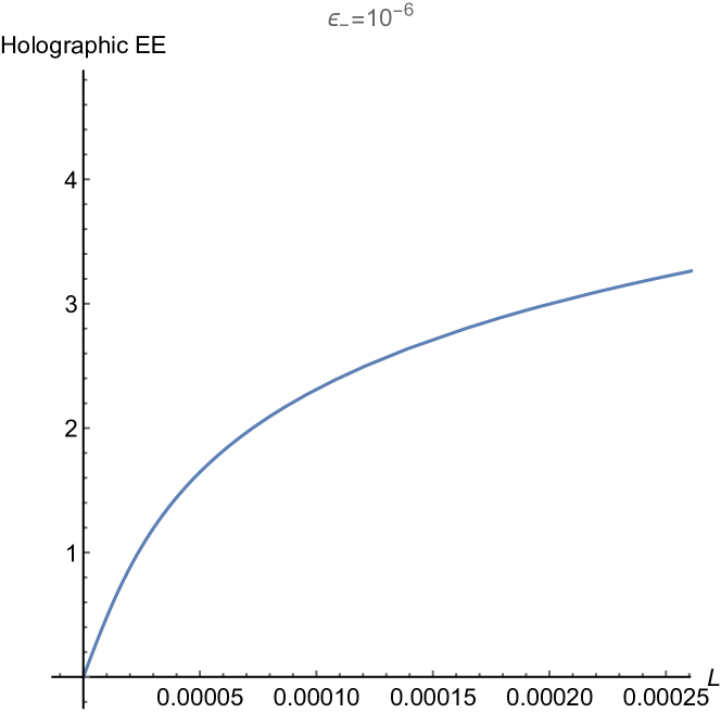
Figure 8: Holographic Entanglement Entropy vs L plot. The values used here are following, $k=10^{4}$, $l_{s}=0.01$ and $\epsilon=10^{-5}$

Here again, we used the value of the warping factor as, $\epsilon_{-}=10^{-6}$ for the same reason mentioned at the end of Sec. 5.2.
One curious fact to note is that the holographic entanglement entropy doesn’t display any on-locality in terms of the UV divergences appearing - for any value of the warping the only type of UV divergence appearing is the log divergence, much akin to a local field theory like CFT₂. This is polar opposite of the pattern of UV divergences appearing in subregion volume complexity (all orders of UV divergences appear there). The fact that the entanglement entropy of a WCFT₂, a highly nonlocal and Lorentz boost violating theory, but has the exact same UV divergence structure as that of the entanglement entropy of a local CFT₂ has been noted in earlier works Castro:2015csg ; Basanisi:2016hsh .

References

- (1) S. Chakraborty, G. Katoch, and S. R. Roy, Holographic complexity of LST and single trace , JHEP 03 (2021) 275, [arXiv:2012.11644].
- (2) S. Chakraborty and A. Hashimoto, Entanglement Entropy for , , deformed holographic CFT, arXiv:2010.15759.
- (3) J. M. Maldacena, The Large N limit of superconformal field theories and supergravity, Int. J. Theor. Phys. 38 (1999) 1113–1133, [hep-th/9711200].
- (4) S. Gubser, I. R. Klebanov, and A. M. Polyakov, Gauge theory correlators from noncritical string theory, Phys. Lett. B 428 (1998) 105–114, [hep-th/9802109].
- (5) E. Witten, Anti-de Sitter space and holography, Adv. Theor. Math. Phys. 2 (1998) 253–291, [hep-th/9802150].
- (6) O. Aharony, S. S. Gubser, J. M. Maldacena, H. Ooguri, and Y. Oz, Large N field theories, string theory and gravity, Phys. Rept. 323 (2000) 183–386, [hep-th/9905111].
- (7) N. Itzhaki, J. M. Maldacena, J. Sonnenschein, and S. Yankielowicz, Supergravity and the large N limit of theories with sixteen supercharges, Phys. Rev. D 58 (1998) 046004, [hep-th/9802042].
- (8) S. Sachdev, Condensed Matter and AdS/CFT, Lect. Notes Phys. 828 (2011) 273–311, [arXiv:1002.2947].
- (9) J. McGreevy, Holographic duality with a view toward many-body physics, Adv. High Energy Phys. 2010 (2010) 723105, [arXiv:0909.0518].
- (10) S. A. Hartnoll, Lectures on holographic methods for condensed matter physics, Class. Quant. Grav. 26 (2009) 224002, [arXiv:0903.3246].
- (11) J. Erlich, E. Katz, D. T. Son, and M. A. Stephanov, QCD and a holographic model of hadrons, Phys. Rev. Lett. 95 (2005) 261602, [hep-ph/0501128].
- (12) L. Da Rold and A. Pomarol, Chiral symmetry breaking from five dimensional spaces, Nucl. Phys. B 721 (2005) 79–97, [hep-ph/0501218].
- (13) A. Karch, E. Katz, D. T. Son, and M. A. Stephanov, Linear confinement and AdS/QCD, Phys. Rev. D 74 (2006) 015005, [hep-ph/0602229].
- (14) S. Ryu and T. Takayanagi, Holographic derivation of entanglement entropy from AdS/CFT, Phys. Rev. Lett. 96 (2006) 181602, [hep-th/0603001].
- (15) V. E. Hubeny, M. Rangamani, and T. Takayanagi, A Covariant holographic entanglement entropy proposal, JHEP 07 (2007) 062, [arXiv:0705.0016].
- (16) X. Dong, The Gravity Dual of Renyi Entropy, Nature Commun. 7 (2016) 12472, [arXiv:1601.06788].
- (17) B. Swingle, Entanglement Renormalization and Holography, Phys. Rev. D 86 (2012) 065007, [arXiv:0905.1317].
- (18) G. Penington, Entanglement Wedge Reconstruction and the Information Paradox, JHEP 09 (2020) 002, [arXiv:1905.08255].
- (19) A. Almheiri, R. Mahajan, J. Maldacena, and Y. Zhao, The Page curve of Hawking radiation from semiclassical geometry, JHEP 03 (2020) 149, [arXiv:1908.10996].
- (20) K. Namsrai, Nonlocal quantum field theory and stochastic quantum mechanics, vol. 13 of Fundamental Theories of Physics. Reidel, Dordrecht, Netherlands, 1986.
- (21) A. Sen, BV Master Action for Heterotic and Type II String Field Theories, JHEP 02 (2016) 087, [arXiv:1508.05387].
- (22) G. V. Efimov, Nonlocal quantum field theory, nonlinear interaction Lagrangians, and convergence of the perturbation theory series, Theor. Math. Phys. 2 (1970), no. 3 217–223.
- (23) M. Van Raamsdonk, Comments on quantum gravity and entanglement, arXiv:0907.2939.
- (24) M. Van Raamsdonk, Building up spacetime with quantum entanglement, Gen. Rel. Grav. 42 (2010) 2323–2329, [arXiv:1005.3035].
- (25) J. M. Maldacena, Eternal black holes in anti-de Sitter, JHEP 04 (2003) 021, [hep-th/0106112].
- (26) M. Van Raamsdonk, Lectures on Gravity and Entanglement, in Theoretical Advanced Study Institute in Elementary Particle Physics: New Frontiers in Fields and Strings, pp. 297–351, 2017. arXiv:1609.00026.
- (27) L. Susskind, Computational Complexity and Black Hole Horizons, Fortsch. Phys. 64 (2016) 24–43, [arXiv:1403.5695]. [Addendum: Fortsch.Phys. 64, 44–48 (2016)].
- (28) M. A. Nielsen, A geometric approach to quantum circuit lower bounds, arXiv e-prints (Feb., 2005) quant–ph/0502070, [quant-ph/0502070].
- (29) M. A. Nielsen, M. R. Dowling, M. Gu, and A. C. Doherty, Quantum Computation as Geometry, Science 311 (Feb., 2006) 1133–1135, [quant-ph/0603161].
- (30) R. Jefferson and R. C. Myers, Circuit complexity in quantum field theory, JHEP 10 (2017) 107, [arXiv:1707.08570].
- (31) S. Chapman, M. P. Heller, H. Marrochio, and F. Pastawski, Toward a Definition of Complexity for Quantum Field Theory States, Phys. Rev. Lett. 120 (2018), no. 12 121602, [arXiv:1707.08582].
- (32) R. Khan, C. Krishnan, and S. Sharma, Circuit Complexity in Fermionic Field Theory, Phys. Rev. D 98 (2018), no. 12 126001, [arXiv:1801.07620].
- (33) R.-Q. Yang, Y.-S. An, C. Niu, C.-Y. Zhang, and K.-Y. Kim, Principles and symmetries of complexity in quantum field theory, Eur. Phys. J. C 79 (2019), no. 2 109, [arXiv:1803.01797].
- (34) J. Molina-Vilaplana and A. Del Campo, Complexity Functionals and Complexity Growth Limits in Continuous MERA Circuits, JHEP 08 (2018) 012, [arXiv:1803.02356].
- (35) L. Hackl and R. C. Myers, Circuit complexity for free fermions, JHEP 07 (2018) 139, [arXiv:1803.10638].
- (36) A. Bhattacharyya, P. Caputa, S. R. Das, N. Kundu, M. Miyaji, and T. Takayanagi, Path-Integral Complexity for Perturbed CFTs, JHEP 07 (2018) 086, [arXiv:1804.01999].
- (37) M. Guo, J. Hernandez, R. C. Myers, and S.-M. Ruan, Circuit Complexity for Coherent States, JHEP 10 (2018) 011, [arXiv:1807.07677].
- (38) A. Bhattacharyya, A. Shekar, and A. Sinha, Circuit complexity in interacting QFTs and RG flows, JHEP 10 (2018) 140, [arXiv:1808.03105].
- (39) R.-Q. Yang, Y.-S. An, C. Niu, C.-Y. Zhang, and K.-Y. Kim, More on complexity of operators in quantum field theory, JHEP 03 (2019) 161, [arXiv:1809.06678].
- (40) H. A. Camargo, M. P. Heller, R. Jefferson, and J. Knaute, Path integral optimization as circuit complexity, Phys. Rev. Lett. 123 (2019), no. 1 011601, [arXiv:1904.02713].
- (41) V. Balasubramanian, M. Decross, A. Kar, and O. Parrikar, Quantum Complexity of Time Evolution with Chaotic Hamiltonians, JHEP 01 (2020) 134, [arXiv:1905.05765].
- (42) A. Bhattacharyya, P. Nandy, and A. Sinha, Renormalized Circuit Complexity, Phys. Rev. Lett. 124 (2020), no. 10 101602, [arXiv:1907.08223].
- (43) J. Erdmenger, M. Gerbershagen, and A.-L. Weigel, Complexity measures from geometric actions on Virasoro and Kac-Moody orbits, JHEP 11 (2020) 003, [arXiv:2004.03619].
- (44) P. Bueno, J. M. Magan, and C. Shahbazi, Complexity measures in QFT and constrained geometric actions, arXiv:1908.03577.
- (45) B. Chen, B. Czech, and Z.-z. Wang, Cutoff Dependence and Complexity of the CFT2 Ground State, arXiv:2004.11377.
- (46) M. Flory and M. P. Heller, Complexity and Conformal Field Theory, arXiv:2005.02415.
- (47) M. Flory and M. P. Heller, Conformal field theory complexity from Euler-Arnold equations, arXiv:2007.11555.
- (48) A. R. Brown, D. A. Roberts, L. Susskind, B. Swingle, and Y. Zhao, Holographic Complexity Equals Bulk Action?, Phys. Rev. Lett. 116 (2016), no. 19 191301, [arXiv:1509.07876].
- (49) A. R. Brown, D. A. Roberts, L. Susskind, B. Swingle, and Y. Zhao, Complexity, action, and black holes, Phys. Rev. D 93 (2016), no. 8 086006, [arXiv:1512.04993].
- (50) L. Lehner, R. C. Myers, E. Poisson, and R. D. Sorkin, Gravitational action with null boundaries, Phys. Rev. D 94 (2016), no. 8 084046, [arXiv:1609.00207].
- (51) K. Parattu, S. Chakraborty, B. R. Majhi, and T. Padmanabhan, A Boundary Term for the Gravitational Action with Null Boundaries, Gen. Rel. Grav. 48 (2016), no. 7 94, [arXiv:1501.01053].
- (52) S. Bolognesi, E. Rabinovici, and S. R. Roy, On Some Universal Features of the Holographic Quantum Complexity of Bulk Singularities, JHEP 06 (2018) 016, [arXiv:1802.02045].
- (53) O. Aharony, M. Berkooz, D. Kutasov, and N. Seiberg, Linear dilatons, NS five-branes and holography, JHEP 10 (1998) 004, [hep-th/9808149].
- (54) D. Kutasov, Introduction to little string theory, ICTP Lect. Notes Ser. 7 (2002) 165–209.
- (55) F. Smirnov and A. Zamolodchikov, On space of integrable quantum field theories, Nucl. Phys. B 915 (2017) 363–383, [arXiv:1608.05499].
- (56) A. Cavaglià, S. Negro, I. M. Szécsényi, and R. Tateo, -deformed 2D Quantum Field Theories, JHEP 10 (2016) 112, [arXiv:1608.05534].
- (57) A. Giveon, N. Itzhaki, and D. Kutasov, and LST, JHEP 07 (2017) 122, [arXiv:1701.05576].
- (58) M. Asrat, A. Giveon, N. Itzhaki, and D. Kutasov, Holography Beyond AdS, Nucl. Phys. B 932 (2018) 241–253, [arXiv:1711.02690].
- (59) S. Chakraborty, A. Giveon, N. Itzhaki, and D. Kutasov, Entanglement beyond AdS, Nucl. Phys. B 935 (2018) 290–309, [arXiv:1805.06286].
- (60) S. Chakraborty, Wilson loop in a like deformed , Nucl. Phys. B 938 (2019) 605–620, [arXiv:1809.01915].
- (61) S. Chakraborty and A. Hashimoto, Thermodynamics of , , deformed conformal field theories, JHEP 07 (2020) 188, [arXiv:2006.10271].
- (62) S. Chakraborty, CFT, NS5F1 system and single trace , arXiv:2012.03995.
- (63) S. Chakraborty, A. Giveon, and D. Kutasov, , , and String Theory, J. Phys. A 52 (2019), no. 38 384003, [arXiv:1905.00051].
- (64) S. Chakraborty, A. Giveon, and D. Kutasov, Strings in irrelevant deformations of AdS3/CFT2, JHEP 11 (2020) 057, [arXiv:2009.03929].
- (65) S. Chakraborty, A. Giveon, and D. Kutasov, deformed CFT2 and string theory, JHEP 10 (2018) 057, [arXiv:1806.09667].
- (66) L. Apolo and W. Song, Strings on warped AdS3 via deformations, JHEP 10 (2018) 165, [arXiv:1806.10127].
- (67) M. Alishahiha, Holographic Complexity, Phys. Rev. D 92 (2015), no. 12 126009, [arXiv:1509.06614].
- (68) O. Ben-Ami and D. Carmi, On Volumes of Subregions in Holography and Complexity, JHEP 11 (2016) 129, [arXiv:1609.02514].
- (69) D. Carmi, R. C. Myers, and P. Rath, Comments on Holographic Complexity, JHEP 03 (2017) 118, [arXiv:1612.00433].
- (70) I. R. Klebanov, D. Kutasov, and A. Murugan, Entanglement as a probe of confinement, Nucl. Phys. B 796 (2008) 274–293, [arXiv:0709.2140].
- (71) J. L. Barbon and C. A. Fuertes, Holographic entanglement entropy probes (non)locality, JHEP 04 (2008) 096, [arXiv:0803.1928].
- (72) A. Reynolds and S. F. Ross, Divergences in Holographic Complexity, Class. Quant. Grav. 34 (2017), no. 10 105004, [arXiv:1612.05439].
- (73) A. Akhavan, M. Alishahiha, A. Naseh, and H. Zolfi, Complexity and Behind the Horizon Cut Off, JHEP 12 (2018) 090, [arXiv:1810.12015].
- (74) G. Jafari, A. Naseh, and H. Zolfi, Path Integral Optimization for Deformation, Phys. Rev. D 101 (2020), no. 2 026007, [arXiv:1909.02357].
- (75) H. Geng, Deformation and the Complexity=Volume Conjecture, Fortsch. Phys. 68 (2020), no. 7 2000036, [arXiv:1910.08082].
- (76) J. M. Maldacena and H. Ooguri, Strings in AdS(3) and SL(2,R) WZW model 1.: The Spectrum, J. Math. Phys. 42 (2001) 2929–2960, [hep-th/0001053].
- (77) N. Seiberg and E. Witten, The D1 / D5 system and singular CFT, JHEP 04 (1999) 017, [hep-th/9903224].
- (78) D. Kutasov and N. Seiberg, More comments on string theory on AdS(3), JHEP 04 (1999) 008, [hep-th/9903219].
- (79) S. Forste, A Truly marginal deformation of SL(2, R) in a null direction, Phys. Lett. B 338 (1994) 36–39, [hep-th/9407198].
- (80) D. Israel, C. Kounnas, and M. P. Petropoulos, Superstrings on NS5 backgrounds, deformed AdS(3) and holography, JHEP 10 (2003) 028, [hep-th/0306053].
- (81) A. Giveon, D. Kutasov, E. Rabinovici, and A. Sever, Phases of quantum gravity in AdS(3) and linear dilaton backgrounds, Nucl. Phys. B 719 (2005) 3–34, [hep-th/0503121].
- (82) S. Chakraborty, A. Giveon, and D. Kutasov, , black holes and negative strings, JHEP 09 (2020) 057, [arXiv:2006.13249].
- (83) O. Aharony, A. Giveon, and D. Kutasov, LSZ in LST, Nucl. Phys. B 691 (2004) 3–78, [hep-th/0404016].
- (84) J. L. Karczmarek and C. Rabideau, Holographic entanglement entropy in nonlocal theories, JHEP 10 (2013) 078, [arXiv:1307.3517].
- (85) N. Shiba and T. Takayanagi, Volume Law for the Entanglement Entropy in Non-local QFTs, JHEP 02 (2014) 033, [arXiv:1311.1643].
- (86) D.-W. Pang, Holographic entanglement entropy of nonlocal field theories, Phys. Rev. D 89 (2014), no. 12 126005, [arXiv:1404.5419].
- (87) S. Minwalla and N. Seiberg, Comments on the IIA (NS)five-brane, JHEP 06 (1999) 007, [hep-th/9904142].
- (88) A. Belin, R. C. Myers, S.-M. Ruan, G. Sárosi, and A. J. Speranza, Does Complexity Equal Anything?, Phys. Rev. Lett. 128 (2022), no. 8 081602, [arXiv:2111.02429].
- (89) T. Azeyanagi, D. M. Hofman, W. Song, and A. Strominger, The Spectrum of Strings on Warped AdS S3, JHEP 04 (2013) 078, [arXiv:1207.5050].
- (90) S. Detournay, T. Hartman, and D. M. Hofman, Warped Conformal Field Theory, Phys. Rev. D 86 (2012) 124018, [arXiv:1210.0539].
- (91) D. M. Hofman and B. Rollier, Warped Conformal Field Theory as Lower Spin Gravity, Nucl. Phys. B 897 (2015) 1–38, [arXiv:1411.0672].
- (92) A. Bhattacharyya, G. Katoch, and S. R. Roy, Complexity of warped conformal field theory, arXiv:2202.09350.
- (93) D. Anninos, J. Samani, and E. Shaghoulian, Warped Entanglement Entropy, JHEP 02 (2014) 118, [arXiv:1309.2579].
- (94) A. Castro, D. M. Hofman, and N. Iqbal, Entanglement Entropy in Warped Conformal Field Theories, JHEP 02 (2016) 033, [arXiv:1511.00707].
- (95) L. Basanisi and S. Chakrabortty, Holographic Entanglement Entropy in NMG, JHEP 09 (2016) 144, [arXiv:1606.01920].
- (96) M. Asrat, Entropic –functions in deformations, Nucl. Phys. B 960 (2020) 115186, [arXiv:1911.04618].
- (97) M. Asrat and J. Kudler-Flam, , the entanglement wedge cross section, and the breakdown of the split property, Phys. Rev. D 102 (2020), no. 4 045009, [arXiv:2005.08972].
- (98) A. Al Balushi, R. A. Hennigar, H. K. Kunduri, and R. B. Mann, Holographic complexity of rotating black holes, JHEP 05 (2021) 226, [arXiv:2010.11203].
- (99) A. Bernamonti, F. Bigazzi, D. Billo, L. Faggi, and F. Galli, Holographic and QFT complexity with angular momentum, JHEP 11 (2021) 037, [arXiv:2108.09281].
- (100) L. Apolo and W. Song, TsT, black holes, and + + , JHEP 04 (2022) 177, [arXiv:2111.02243].
- (101) A. Hamilton, D. N. Kabat, G. Lifschytz, and D. A. Lowe, Local bulk operators in AdS/CFT: A Boundary view of horizons and locality, Phys. Rev. D 73 (2006) 086003, [hep-th/0506118].
- (102) A. Hamilton, D. N. Kabat, G. Lifschytz, and D. A. Lowe, Holographic representation of local bulk operators, Phys. Rev. D 74 (2006) 066009, [hep-th/0606141].
- (103) A. Hamilton, D. N. Kabat, G. Lifschytz, and D. A. Lowe, Local bulk operators in AdS/CFT: A Holographic description of the black hole interior, Phys. Rev. D 75 (2007) 106001, [hep-th/0612053]. [Erratum: Phys.Rev.D 75, 129902 (2007)].
- (104) K. Goto, H. Marrochio, R. C. Myers, L. Queimada, and B. Yoshida, Holographic Complexity Equals Which Action?, JHEP 02 (2019) 160, [arXiv:1901.00014].
- (105) C. N. Pope, “Lectures on Kaluza-Klein theory.” http://www.phys.ens.fr/~cremmer/IHP/ihpprogpope.html, Institut Henri Poincaré (IHP) (November 2000).