Estimating the Spectral Density at Frequencies Near Zero

Abstract

Estimating the spectral density function $f(w)$ for some $w\in[-\pi,\pi]$ has been traditionally performed by kernel smoothing the periodogram and related techniques. Kernel smoothing is tantamount to local averaging, i.e., approximating $f(w)$ by a constant over a window of small width. Although $f(w)$ is uniformly continuous and periodic with period $2\pi$, in this paper we recognize the fact that $w=0$ effectively acts as a boundary point in the underlying kernel smoothing problem, and the same is true for $w=\pm\pi$. It is well-known that local averaging may be suboptimal in kernel regression at (or near) a boundary point. As an alternative, we propose a local polynomial regression of the periodogram or log-periodogram when $w$ is at (or near) the points 0 or $\pm\pi$. The case $w=0$ is of particular importance since $f(0)$ is the large-sample variance of the sample mean; hence, estimating $f(0)$ is crucial in order to conduct any sort of inference on the mean.

Keywords Flat-top lag-windows, Function Estimation, Kernel smoothing, Local Polynomials, Long-run variance, Sample mean

1 Introduction

Many applications of time series analysis involve the nonparametric estimation of the spectral density function $f(w)$ as some point $w\in[-\pi,\pi]$; examples include astronomy, economics, electrical engineering, physics, etc. The prevalent spectral estimation method in the literature goes back to Bartlett (1946, 1948) and Daniell (1946), and can be represented in two equivalent ways: (a) kernel smoothing of the periodogram, and (b) tapered Fourier series of the sample autocovariances.

By the late 1950s the subject was already well understood, as the early books by Grenander and Rosenblatt (1957), and Blackman and Tukey (1959) demonstrate. Influential papers at the time include Hannan (1957, 1958), Parzen (1957, 1961), and Priestley (1962). More recent advances include smoothing the log-periodogram of Wahba (1980), smoothing with the trapezoidal ‘flat-top’ lag-window of Politis and Romano (1995), local polynomial smoothing of the periodogram by Fan and Kreutzberger (1998), and the thresholded Fourier series of Paparoditis and Politis (2012). The book-length treatments in Hannan (1970), Brillinger (1981), Priestley (1981), Brockwell and Davis (1991), Rosenblatt (1985), Percival and Walden (1993), and McElroy and Politis (2020) contain a vast number of additional references.

Kernel smoothing of the periodogram is tantamount to local averaging, i.e., approximating $f(w)$ by a constant over a window of small width. Although the spectral density function $f(w)$ is uniformly continuous and periodic with period $2\pi$, in this paper we recognize the fact that $w=0$ effectively acts as a boundary point in the underlying kernel smoothing problem, and the same is true for $w=\pm\pi$. It is well-known that local averaging may be suboptimal in kernel regression at (or near) a boundary point. As an alternative, we propose a local polynomial regression of the periodogram (or log-periodogram) when $w$ is at (or near) the points 0 or $\pm\pi$. The case $w=0$ is of particular importance since $f(0)$ is the large-sample variance of the sample mean; hence, estimating $f(0)$ is crucial in order to conduct inference on the mean. Due to the symmetries of $f(w)$, the recommended polynomial regression at the two boundaries entails a quadratic without a linear term.

The remainder of the paper is structured as follows. In Section 2.1, traditional spectral estimators are reviewed, and the new method is proposed in Section 2.2. Section 2.3 describes how the same ideas are applicable to spectral estimation near the two boundaries. Section 3 studies the asymptotic performance of the new proposal, and calculates the optimal bandwidth. Section 4.1 discusses the positivity issue and proposes a log-periodogram estimator that is designed to positive, while Section 4.2 shows how to combine the boundary estimators with a traditional spectral estimator valid for interior points. Section 4.3 makes extensions to nonstationary time series with time-varying mean function. Section 5 presents our proposed method of data-based bandwith choice, and includes results of an extensive finite-sample simulation experiment; the simulations required several months of computer time on a 20-core workstation dedicated to statistical computing. Finally, Section 6 gives two real data applications: the U.S. Gross Domestic Product (GDP) and the Global Land-Ocean Temperature Index (GLOTI). An array of tables and figures is deferred to the Supplement (https://mathweb.ucsd.edu/~politis/PAPER/LocalQuadSupp.pdf).

2 Spectral density estimation

Suppose $X_{1},\ldots,X_{n}$ are observations from the (strictly) stationary real-valued sequence $\{X_{t},t\in{\bf Z}\}$ having mean $\mu=EX_{t}$ and autocovariance sequence $\gamma(k)=E(X_{t}-\mu)(X_{t+|k|}-\mu)$, where both $\mu$ and $\gamma(\cdot)$ are unknown; also define the autocorrelation sequence $\rho(k)=\gamma(k)/\gamma(0)$. Typical estimators of $\mu$ and $\gamma(k)$ are the sample mean $\bar{X}_{n}=n^{-1}\sum_{i=1}^{n}X_{i}$ and sample autocovariance $\hat{\gamma}(k)=n^{-1}\sum_{i=1}^{n-|k|}(X_{i}-\bar{X}_{n})(X_{i+|k|}-\bar{X}_{n})$ respectively; $\hat{\gamma}(k)$ is defined to be zero when $|k|\geq n$. Our objective is the nonparametric estimation of the spectral density function $f(w)=\sum_{s=-\infty}^{\infty}e^{iws}\gamma(s)$ assuming that the infinite sum is well-defined. Consider the assumption:

Assumption A$(p)$: The spectral density $f(w)$ is $p$-times continuously differentiable for all real $w$. From here on and throughout this paper, we will assume Assumption A($p$) holds for some $p\geq 2$. Note that $f(w)$ (and its derivatives) are periodic functions with period $2\pi$, and $f(w)$ has even symmetry, i.e., $f(w)=f(-w)$; hence, we can focus on estimating it for $w\in[0,\pi]$ only. It is easy to see that if $\sum_{s=-\infty}^{\infty}|s|^{p}|\gamma(s)|<\infty$ for some non-negative integer $p$, then Assumption A$(p)$ holds true; see e.g. Proposition 6.1.5 of McElroy and Politis (2020).

2.1 Traditional spectral estimation

The traditional kernel estimator of $f(w)$ in its Fourier series form is defined as

$$\widehat{f}(w)=\sum_{s=-\infty}^{\infty}e^{iws}\lambda(s/M)\widehat{\gamma}(s),$$ (1)

where the lag-window $\lambda(s)$ is a bounded, square-integrable function with even symmetry that satisfies $\lambda(0)=1$. Suppose that $\lambda(s)$ has $q$ continuous derivatives at the origin; if $\lambda^{(k)}(0)=0$ for $k=1,\ldots,q-1$, then $\lambda(s)$ is said to have order equal to $q$. Popular choices for 2nd order lag-windows have been proposed by Parzen (1961) and Priestley (1962).

The periodogram is defined as $I(w)=\sum_{s=-\infty}^{\infty}e^{iws}\widehat{\gamma}(s)$. By the convolution formula — see Proposition 6.1.11 of McElroy and Politis (2020) — it follows that we can alternatively express $\widehat{f}(w)$ by means of smoothing the periodogram, i.e.,

$$\widehat{f}(w)=\frac{1}{2\pi}\int_{-\pi}^{\pi}\Lambda_{M}(s)I(w+s)ds,$$ (2)

where $\Lambda_{M}(w)=\sum_{s=-\infty}^{\infty}e^{iws}\lambda(s/M)$ is the so-called spectral kernel. The integral in eq. (2) is practically approximated by a Riemann sum over the Fourier frequencies $w_{j}=2\pi j/n$, i.e.,

$$\hat{f}(w)\approx\frac{1}{n}\sum_{j\in J_{n}}\Lambda_{M}(w_{j})I(w+w_{j}),$$ (3)

where the error in the approximation is $O(1/n)$. The index set $J_{n}$ consists of $n$ consecutive integers as follows: $J_{n}=\{-\frac{n-1}{2},\ldots,0,\ldots,\frac{n-1}{2}\}$ if $n$ is odd, and $J_{n}=\{-\frac{n}{2}+1,\ldots,0,\ldots,\frac{n}{2}\}$ if $n$ is even.

It is well known that under regularity conditions

$$Var[\hat{f}(w)]=\eta(w)f^{2}(w)\frac{M}{n}\int_{-\infty}^{\infty}\lambda^{2}(s)ds+o\left(\frac{M}{n}\right)$$ (4)

as $n\to\infty$, $M\to\infty$ but $\frac{M}{n}\to 0$; see e.g. Rosenblatt (1984), Shao and Wu (2007), or Ch. 9 of McElroy and Politis (2020). The function $\eta(w)=2$ if $w$ is zero or an integer multiple of $\pi$; otherwise, $\eta(w)=1$. Furthermore, under Assumption A$(p)$ for some $p\geq 2$ we have

$$Bias[\hat{f}(w)]=O\left(M^{-\min(p,q)}\right),$$ (5)

where $q$ is the order of the kernel. It is apparent that if $f(w)$ is very smooth, i.e., possessing a large number of derivatives, it would be advantageous to use a high-order kernel.

A more recent development is the use of flat-top lag-windows; see Paradigm 9.9.1 of McElroy and Politis (2020). Flat-top lag-windows have been shown to achieve the optimal rate of convergence in a given smoothness class by automatically adapting to the underlying smoothness of the true spectral density. A general ‘flat-top’ lag-window is defined as

$$\lambda_{g,c}(x)=\begin{cases}1\quad\mbox{if}\,|x|\leq c\\ g(x)\quad\mbox{else};\end{cases}$$ (6)

here $c>0$ is a shape parameter, and $g:{\rm I}\!{\rm R}\to[-1,1]$ is a symmetric function, continuous at all but a finite number of points, and satisfying $g(c)=1$, and $\int_{c}^{\infty}g^{2}(x)dx<\infty$. Note that a flat-top lag-window has infinite order, as all its derivatives vanish at the origin. The trapezoidal lag-window of Politis and Romano (1995), given by $\lambda(x)=\left(\min\{1,2(1-|x|)\}\right)^{+}$, is a prominent member of the flat-top family; here, $(x)^{+}=\max(x,0)$.

It has been found—see e.g. Politis (2001, 2003, 2011)—that estimator (1) using a flat-top lag-window achieves the optimal rate of convergence in a given smoothness class; these optimal rates are delineated in Samarov (1977). Hence, a flat-top lag-window estimator exhibits adaptivity to the (unknown) degree of smoothness of the underlying true spectral density; the degree of smoothness can be quantified by the rate of the decay of the autocovariance. Perhaps more importantly, these optimal rates are (almost) achieved even when an empirical data-dependent choice of the bandwidth $M$ is employed—see Politis (2003, 2011).

Remark 2.1

A minor complication is that flat-top lag-windows are not positive definite, i.e., using them does not ensure that $\hat{f}(w)$ will be non-negative almost surely. Since $f(w)\geq 0$ always, an easy fix is to take the positive part of $\hat{f}(w)$, i.e., define the modified estimator $\hat{f}^{+}(w)=\max(\hat{f}(w),0)$. Alternative corrections for positivity are discussed in Appendix A of McMurry and Politis (2015).

2.2 Improved spectral estimation at the origin

Consider for a moment a different setup, where we have data $Y_{1},\ldots,Y_{n}$ from the nonparametric regression model

$$Y_{j}=f(x_{j})+\sigma(x_{j})\epsilon_{j},$$ (7)

where the errors $\epsilon_{i}$ are independent, identically distributed (i.i.d.) with mean zero, and variance one. Here, $f(x)$ and $\sigma(x)$ are smooth (but otherwise unknown) functions with compact support $[c_{1},c_{2}]$. Kernel smoothing, i.e., local averaging of the $Y_{i}$ data, is a fundamental way to estimate the function $f(x)$ for some $x\in[c_{1},c_{2}]$.

Local averaging is tantamount to approximating $f(x)$ by a constant over a small window of the type $[x-h,x+h]$; here, $h$ is a small positive number called the bandwidth. It is well known that local linear (and local polynomial) fitting outperforms local averaging when either the point of interest $x$ is in a region where few design points $x_{j}$ are found, or $x$ is near (or on) one of the boundary points $c_{1},c_{2}$; see Fan and Gijbels (1996) and the references therein.

Recall that the periodogram ordinates $I(w_{j})$ for $j\in J_{n}$ are approximately independent. The asymptotic distribution of $I(w)/f(w)$ is Exponential with mean one if $w\in(0,\pi)$; if $w=\pm\pi$, then $I(w)/f(w)$ is asymptotically chi-square with one degree of freedom. Note that $I(0)=0$ identically; see Corollary 9.7.5 of McElroy and Politis (2020). That said, it is apparent that eq. (3) is tantamount to applying local averaging on the nonparametric regression (7) with $Y_{j}=I(w_{j})$, $\sigma(w_{j})=f(w_{j})$, and the $\epsilon_{j}$ being (approximately) i.i.d. Exponential with mean one.

Although Fan and Kreutzberger (1998) did work out the local polynomial method of estimating $f(w)$ for $w\in(0,\pi)$, their results were not appreciably better than the local averaging of eq. (3). The intuitive reason is that the design points are uniformly spaced $w_{j}=2\pi j/n$, which makes local linear fitting equivalent to simple local averaging.

Since $f(w)$ is continuous over $[-\infty,\infty]$ and periodic with period $2\pi$, it has been thought that its nonparametric estimation does not suffer from boundary effects; this, however, is not entirely correct. To see why, focus on the case $w=0$; since $I(0)=0$, the estimator $\hat{f}(0)$ from eq. (3) involves averaging periodogram ordinates to the left and to the right of the origin. But $I(w)$ has even symmetry, and is periodic with period $2\pi$ as well. Because of the symmetry $I(w)=I(-w)$, the estimator $\hat{f}(0)$ from eq. (3) is tantamount to a one-sided average, i.e.,

$$\hat{f}(0)\approx\frac{1}{n}\sum_{j\in J_{n}}\Lambda_{M}(w_{j})I(w_{j})=\frac{2}{n}\sum_{j\in J_{n}^{+}}\Lambda_{M}(w_{j})I(w_{j}),$$ (8)

where $J_{n}^{+}$ is the subset of positive indices belonging to $J_{n}$; this actually explains the doubling of the variance when $w=0$ in eq. (4) since the effective sample size is halved due to the symmetry.

Therefore, $w=0$ effectively acts as a boundary point in nonparametric regression of periodogram ordinates. The same is true for the points $w=\pm\pi$ due to the periodicity of $I(w)$. Hence, we may propose local polynomial fitting of periodogram ordinates in order to estimate $f(w)$ when $w$ is zero, or an integer multiple of $\pi$. Because of the even symmetry (and periodicity) of $f(w)$, local linear fitting would again be equivalent to local averaging when $w=0$ or $\pm\pi$. A local quadratic (without a linear term) can be fitted instead; setting $h=2\pi\delta$, for a small $\delta\in(0,.5)$, we may use the Taylor approximations

$$f(w)\approx a_{0}+b_{0}w^{2}\ \ \mbox{for}\ \ w\in[-2\pi\delta,2\pi\delta]$$ (9)

$$\mbox{and}\ \ f(w)\approx a_{1}+b_{1}(w-\pi)^{2}\ \ \mbox{for}\ \ w\in[\pi-2\pi\delta,\pi+2\pi\delta].$$ (10)

Since $f(-\pi)$=$f(\pi)$, we do not have to address the case $w=-\pi$ separately. Our proposal then is summarized in the following algorithm:

Algorithm 2.1

1. Let $\hat{a}_{0}$ and $\hat{b}_{0}$ be the estimators of $a_{0}$ and $b_{0}$ in eq. (9) based on a (possibly weighted) regression of $I(w)$ on an intercept $a_{0}$ and quadratic term $b_{0}w^{2}$. The data to be used in this regression are $I(w_{1}),\ldots,I(w_{m})$, where $w_{m}$ is the largest Fourier frequency less or equal to $2\pi\delta$; since $w_{m}=2\pi m/n\leq 2\pi\delta$, it follows that $m=[\delta n]$, where $[\cdot]$ denotes the integer part. Explicit formulas for $\hat{a}_{0}$ and $\hat{b}_{0}$ are provided in Section 3.

2. Similarly, $\hat{a}_{1}$ and $\hat{b}_{1}$ are the estimators of $a_{1}$ and $b_{1}$ in eq. (10) based on a (possibly weighted) regression of $I(w)$ on an intercept $a_{1}$ and quadratic term $b_{1}(w-\pi)^{2}$. The data to be used in this regression are the $I(w_{j})$ with indices corresponding to the $m$ largest elements of set $J_{n}$.

3. Finally, $\tilde{f}(0)=\hat{a}_{0}$ is the proposed new estimator of $f(0)$, and $\tilde{f}(\pi)=\hat{a}_{1}$ is the proposed estimator of $f(\pi)$. As will be shown in Section 3, to achieve consistent estimation in either of the above cases, we would need $\delta\to 0$ but $\delta n\to\infty$ as $n\to\infty$, which is equivalent to $m\to\infty$ but with $m/n\to 0$.

Remark 2.2

Marron and Ruppert (1994) studied in detail the problem of nonparametric estimation of a probability density at its boundaries. The case of the nonparametric spectral density estimator $\widehat{f}(w)$ using a non-negative spectral kernel $\Lambda_{M}$ is completely analogous. In both cases, the bias of $\widehat{f}(w)$ is of order $f^{\prime\prime}(w)/M^{2}$ if $w$ is an interior point. Furthermore, the first term in the expansion of the bias of $\widehat{f}(\theta)$ is of order $f^{\prime}(\theta)/M$, where $\theta$ is one of the “boundary” points, i.e., $\theta=0$ or $\pm\pi$. Note, however, that because of the even symmetry (and periodicity) of $f(w)$, we have $f^{\prime}(\theta)=0$. Therefore, the bias of $\widehat{f}(w)$ is of order $O(M^{-2})$ for all $w$, even at the boundary. It is perhaps for this reason that spectral estimation has not been identified in the past literature as having a boundary issue. Indeed, the situation at the boundary could be better described as a boundary opportunity rather than a boundary problem.

Recall that we motivated the presence of the boundary issue by the fact that the variance of $\widehat{f}(w)$ is doubled when $w$ is at the boundary; however, there is an issue with the bias as well. Note that $|Bias(\widehat{f}(w))\approx|f^{\prime\prime}(w)|/M^{2}$; furthermore, $|f^{\prime\prime}(w)|$ has a (local) maximum when $w=0$ or $\pm\pi$, as it corresponds to points of maximum curvature of $f(w)$. Hence, there is an issue with the bias as well although—like in the variance—it does not affect the rate of convergence; it just affects the constants in the bias and variance asymptotic expansions. All this goes to show that estimating ${f}(w)$ for $w=0$ or $\pm\pi$ may require more scrutiny, especially since estimating ${f}(0)$ is fundamental for time series inference.

To give a different analogy, in regression we often fit linear trends, globally (as in straight line regression) or locally (as in local linear fitting of nonparametric regression). If it is known that a regression function has a quadratic behavior (either globally or locally), then it behooves us to fit a quadratic instead. For example, in looking for the maximum (or minimum) of a regression function, it is standard practice to fit a (local) quadratic; see e.g. Myers et al. (2016). Hence, our proposal of local quadratic fitting to estimate ${f}(w)$ for $w$ at the boundaries is natural, since we know that ${f}(w)$ has a local maximum or minimum for $w=0$ or $\pm\pi$. As we will see in Section 3, the above simple Algorithm of local quadratic fitting leads to a bias of order $O(M^{-4})$ at the boundary points, thus taking advantage of the aforementioned boundary opportunity.

If Assumption A($p$) holds with $p>2$, then a higher order polynomial (with only even powers) could also be used instead of the simple quadratics (9) and (10), the goal again being to estimate the respective intercept terms; the details are straightforward and thus omitted.

2.3 Improved spectral estimation near the two boundaries

The dichotomous asymptotic behavior of $\hat{f}(w)$ according to whether $w=0$ or not obfuscates the need for a special treatment of $\hat{f}(w)$ where $w$ is very close to zero (or $\pi$ for that matter). For example, the estimator $\hat{f}(w_{1})$ faces the same boundary problems described in eq. (8), namely $\hat{f}(w_{1})$ is (for the most part) a one-sided average. Consequently, $Var[\hat{f}(w_{1})]\approx Var[\hat{f}(0)]$, which is double the variance of $\hat{f}(w)$ at a point $w$ far from the boundary.

Such boundary issues are shared by all $\hat{f}(w_{j})$ for $j=1,\ldots,m$, as well as all $\hat{f}(w_{j})$ with indices corresponding to the $m$ largest elements of set $J_{n}$; here, $m$ is as defined in Algorithm 2.1(i). However, the fitted equations (9) and (10) give us a way to address all boundary issues in a unified way. We now define an estimated function $\tilde{f}(w)$ for all $w\in[-\pi,\pi]$ by the following construction. We first define it over the non-negative Fourier frequencies, so let:

$$\tilde{f}(w_{j})=\begin{cases}\hat{a}_{0}+\hat{b}_{0}w_{j}^{2}\quad\mbox{if}\,j=0,1,\ldots,m\\ 0\qquad\qquad\mbox{if}\,j=m+1,\ldots,[n/2]-m\\ \hat{a}_{1}+\hat{b}_{1}(w_{j}-\pi)^{2}\quad\mbox{if}\,j=[n/2]-m+1,\ldots,[n/2].\end{cases}$$ (11)

We then extend to negative Fourier frequencies by symmetry, i.e., letting $\tilde{f}(w_{j})=\tilde{f}(-w_{j})$ if $w_{j}<0$. Finally, we extend to all of $[-\pi,\pi]$ as follows: if $w$ is not a Fourier frequency, let $\tilde{f}(w)=\tilde{f}(w_{j^{*}})$ where $w_{j^{*}}$ is the Fourier frequency closest to $w$.

3 Asymptotic performance

The spectral density $f(w)$ is assumed to be smooth, i.e., possessing a number of derivatives, as postulated in Assumption A$(p)$ of Section 2. Therefore, $f(w)$ admits a Taylor expansion of an appropriate order at any frequency $\theta$ of interest. At the boundary points, i.e., when $\theta=0$ or $\pm\pi$, the spectral density is an even function of $w-\theta$, and hence the Taylor expansion only involves even order terms. Assuming Assumption A$(4)$, we can write

$$f(w)=f(\theta)+\frac{1}{2}f^{(2)}(\theta)\,{(w-\theta)}^{2}+\frac{1}{4!}f^{(4)}(\theta)\,{(w-\theta)}^{4}+o({(w-\theta)}^{4}),$$ (12)

where $o(1)$ denotes terms tending to zero as $|w-\theta|\rightarrow 0$. We will use this expansion to analyze the bias and variance of the estimator $\tilde{f}(w)$, focusing on the cases that $\theta=0$ or $\pi$.

3.1 Fitting via Ordinary Least Squares (OLS)

The Ordinary Least Squares (OLS) regression estimator of $a_{0}$ and $b_{0}$ (or $a_{1}$ and $b_{1}$) at any of the boundary frequencies $\theta$ takes the form ${({\bf X}^{\prime}{\bf X})}^{-1}{\bf X}^{\prime}{\bf Y}$, where ${\bf X}$ has a first column of $m$ ones and a second column of $m$ values ${(\theta-w_{j})}^{2}$. These $w_{j}$ are the Fourier frequencies falling in the interval $[\theta-2\pi\delta,\theta+2\pi\delta]\cap(0,\pi]$. Also ${\bf Y}$ is a vector with entries $I(w_{j})$, the periodogram evaluated at this band of Fourier frequencies. To determine the Fourier frequencies that are used, note that by even symmetry at the boundaries we only need to focus on the interval $[0,\pi]$, and the scenario for $\theta=-\pi$ is the same as for $\theta=\pi$. Hence, for $\theta=0$ we consider the set of $w_{j}\in(0,2\pi\delta]$, or $1\leq j\leq m$ with $m=[\delta n]$. Note that we don’t use $j=0$ in the regression, because typically the periodogram will have been mean-centered, implying that $I(w_{0})=0$. For $\theta=\pi$, we consider the set of $w_{j}\in[\theta-2\pi\delta,\pi]$, or $[n/2]-m+1\leq j\leq[n/2]$. We can take the lower bound to be $[n/2-n\delta]$ instead of $[n/2]-m+1$ for purposes of asymptotic analysis.

Now $w_{j}=2\pi j/n$, and we will approximate ${({\bf X}^{\prime}{\bf X})}^{-1}$ using summation formulas; for either $\theta=0$ or $\theta=\pi$ we have the approximation (it is exact if $\theta=0$)

$${\bf X}^{\prime}{\bf X}=\left[\begin{array}[]{cc}m&\sum_{j}{(\theta-w_{j})}^{2}\\ \sum_{j}{(\theta-w_{j})}^{2}&\sum_{j}{(\theta-w_{j})}^{4}\end{array}\right]\approx\left[\begin{array}[]{cc}m&{(2\pi/n)}^{2}\sum_{j=1}^{m}j^{2}\\ {(2\pi/n)}^{2}\sum_{j=1}^{m}j^{2}&{(2\pi/n)}^{4}\sum_{j=1}^{m}j^{4}\end{array}\right].$$

Taking the limit as $n\rightarrow\infty$ of $m^{-1}{\bf X}^{\prime}{\bf X}$ yields the matrix $Q$:

$$Q=\left[\begin{array}[]{cc}1&{(2\pi\delta)}^{2}/3\\ {(2\pi\delta)}^{2}/3&{(2\pi\delta)}^{4}/5\end{array}\right].$$

Similarly,

$$m^{-1}{\bf X}^{\prime}{\bf Y}=\left[\begin{array}[]{c}m^{-1}\sum_{j}I(w_{j})\\ m^{-1}\sum_{j}I(w_{j}){(\theta-w_{j})}^{2}\end{array}\right].$$

Let the region $A$ denote either $[0,2\pi\delta]$ or $[\pi-2\pi\delta,\pi]$, depending on whether $\theta=0$ or $\theta=\pi$. Then asymptotically the estimator takes the form

$$\tilde{f}(w) =[1,{(\theta-w)}^{2}]\,{({\bf X}^{\prime}{\bf X})}^{-1}{\bf X}^{\prime}{\bf Y}$$

$$\approx[1,{(\theta-w)}^{2}]\,Q^{-1}\,\left[\begin{array}[]{c}m^{-1}\sum_{j}I(w_{j})\\ m^{-1}\sum_{j}I(w_{j}){(\theta-w_{j})}^{2}\end{array}\right]$$

$$=m^{-1}\sum_{j}[1,{(\theta-w)}^{2}]\,Q^{-1}\,{[1,{(\theta-w_{j})}^{2}]}^{\prime}\,I(w_{j})$$

$$\approx\frac{1}{2\pi\delta}\int_{A}[1,{(\theta-w)}^{2}]\,Q^{-1}\,{[1,{(\theta-\lambda)}^{2}]}^{\prime}\,I(\lambda)\,d\lambda.$$

Comparing with Remark 9.8.2 of McElroy and Politis (2020), it is apparent that the above estimator is a so-called spectral mean, i.e., has the form $\langle g_{2\delta}(\cdot,w)I\rangle$ with weighting function

$$g_{2\delta}(\lambda,w)=\delta^{-1}[1,{(\theta-w)}^{2}]\,Q^{-1}\,{[1,{(\theta-\lambda)}^{2}]}^{\prime},$$ (14)

which has been defined on $[0,\pi]$ only, i.e., on $[-\pi,0]$ it is defined to be zero. Here, $\langle\cdot\rangle$ denotes integration over $[-\pi,\pi]$, followed by division by $2\pi$, so that $\tilde{f}(w)\approx\langle g_{2\delta}(\cdot,w)I\rangle$.

The asymptotic theory is then given by Theorem 9.6.6 of McElroy and Politis (2020), which assumes a linear process; however, cumulant conditions as in Brillinger (1981) can provide the same result. Let the tri-spectral density of the data process $\{X_{t}\}$ be denoted by

$$F(\omega,\lambda,\theta)=\sum_{h,k,\ell}\gamma(h,k,\ell)\exp\{-i(h\omega+k\lambda+\ell\phi)\},$$

where $\gamma(h,k,\ell)=\mbox{cum}(X_{t},X_{t+h},X_{t+k},X_{t+\ell})$ is the fourth-order autocumulant function of the process. The following Central Limit Theorem (CLT) summarizes the asymptotic properties of the estimator; the result is not limited to $g_{2\delta}(\lambda,w)$ having the form of eq. (14).

Theorem 3.1

Suppose $\{X_{t}\}$ is a strictly stationary time series that is either a linear process (with square summable MA($\infty$) coefficients, and inputs with finite fourth moment) or has autocumulant functions satisfying the summability condition (B1) of Taniguchi and Kakizawa (2000, p.55). Then, as $n\rightarrow\infty$

$$\sqrt{n}\,(\langle g_{2\delta}(\cdot,w)I\rangle-\langle g_{2\delta}(\cdot,w)f\rangle)\stackrel{{\scriptstyle{\cal L}}}{{\Longrightarrow}}\mathcal{N}\left(0,\langle{g_{2\delta}(\cdot,w)}^{2}f^{2}\rangle+G\right),$$

$$\mbox{where }\ \ G=\frac{1}{{(2\pi)}^{2}}\int\int g_{2\delta}(\phi,w)g_{2\delta}(\lambda,w)F(-\phi,\lambda,-\lambda)\,d\lambda d\phi.$$

Proof of Theorem 3.1.

Once the conditions are checked, this result directly follows from Lemma 3.1.1.(ii) of Taniguchi and Kakizawa (2000). Note that the first term in the asymptotic variance would normally also involve a term involving the integral of $g_{2\delta}$ multiplied by its reflection about the y-axis; however, this product will be zero, since $g_{2\delta}$ is supported on $[0,\pi]$.     q.e.d.

Remark 3.1

Focusing on the case where $g_{2\delta}(\lambda,w)$ has the form of eq. (14), note that the centering in the above CLT is $\langle g_{2\delta}(\cdot,w)f\rangle$ which is not equal to $f(w)$ in general; hence, there is an asymptotic bias term to be determined. In addition, the asymptotic variance can be cumbersome since the quantity $G$ depends on the tri-spectral density. Note that $G=0$ if $\{X_{t}\}$ is a Gaussian process but it need not vanish in general. In particular, if $\{X_{t}\}$ is a linear process with innovations of kurtosis $\eta$, we have $G=(\eta-3){\langle g_{2\delta}(\cdot,w)f\rangle}^{2}$; see Taniguchi and Kakizawa (2000, pp. 58-59). In this case, $G$ can be estimated by plugging in a consistent estimator of $f(w)$ in this expression.

We now provide an asymptotic analysis of bias and variance in terms of a fixed $\delta$. The familiar situation where the bandwidth $\delta\rightarrow 0$ will be studied in the next subsection, where it is shown that $G$ is of smaller order (as $\delta\rightarrow 0$) than the first term in the variance. With this in mind, we focus just on the first term of the variance so as to develop an expression for the optimal bandwidth; a fixed bandwidth calculation can be most informative, as the pioneering work of Kiefer and Vogelsang (2002, 2005) has shown – see also McElroy and Politis (2013, 2014). For example, in our case at hand, the actual values of $\delta$ that minimize MSE can be as large as $0.15$, and therefore it might not be appropriate to base the optimal selection of $\delta$ on formulas derived under a $\delta\rightarrow 0$ analysis.

Denote the entries of $m^{-1}{\bf X}^{\prime}{\bf X}$ by $c_{0}$ (upper left), $c_{2}$ (upper right), and $c_{4}$ (lower right). For a non-negative integer $p$ define

$$F_{p}=m^{-1}\sum_{j}{(\theta-w_{j})}^{p}{f(w_{j})}^{2}\ \ \mbox{and}\ \ G_{p}=m^{-1}\sum_{j}{(\theta-w_{j})}^{p}f(w_{j}).$$

Proposition 3.1

Suppose $\{X_{t}\}$ satisfies the conditions of Theorem 3.1 such that $G=0$ in the asymptotic variance. Assume (12), and that $n\rightarrow\infty$ but $\delta$ is a fixed value. For $\theta=0$ or $\pi$ we have

$$\mbox{Var}[\tilde{f}(\theta)]=\delta^{-1}n^{-1}\frac{c_{4}^{2}F_{0}-2c_{4}c_{2}F_{2}+c_{2}^{2}F_{4}}{{(c_{4}-c_{2}^{2})}^{2}}+o(n^{-1})\ \ \mbox{and}\ \ \mbox{Bias}[\tilde{f}(\theta)]=\frac{c_{4}G_{0}-c_{2}G_{2}}{c_{4}-c_{2}^{2}}-f(\theta)+O(n^{-1}).$$

Proof of Proposition 3.1.

Here we develop a variance expression that has a better finite-sample approximation then that given in Theorem 3.1. Letting $[a,b]=[1,{(\theta-w)}^{2}]\,{\left[m^{-1}{\bf X}^{\prime}{\bf X}\right]}^{-1}$, we see the estimator is $\tilde{f}(w)=m^{-1}\sum_{j}(a+b{(\theta-w_{j})}^{2})I(w_{j})$. Hence the variance is asymptotically given by $m^{-2}\sum_{j}{(a+b{(\theta-w_{j})}^{2})}^{2}{f(w_{j})}^{2}$. Then

$${\left[m^{-1}{\bf X}^{\prime}{\bf X}\right]}^{-1} =q^{-1}\,\left[\begin{array}[]{cc}c_{4}&-c_{2}\\ -c_{2}&c_{0}\end{array}\right]$$

$$q =c_{4}c_{0}-c_{2}^{2}$$

$$[a,b] =[c_{4}-c_{2}{(\theta-w)}^{2},-c_{2}+c_{0}{(\theta-w)}^{2}]/q$$

$$a+b{(\theta-w_{j})}^{2} =\left((c_{4}-c_{2}{(\theta-w_{j})}^{2})+{(\theta-w)}^{2}(-c_{2}+c_{0}{(\theta-w_{j})}^{2})\right)/q.$$

Focusing on the case $w=\theta$, the asymptotic variance is

$$m^{-2}\sum_{j}{(c_{4}-c_{2}{(\theta-w_{j})}^{2})}^{2}{f(w_{j})}^{2}/q^{2},$$

which simplifies to the stated expression. To address the bias, let $\widetilde{\bf{Y}}$ be defined via replacing the periodogram by the true spectrum in ${\bf Y}$. So, taking the expectation of the estimator yields

$$E\widetilde{f}(w) =[1,{(\theta-w)}^{2}]\,{({\bf X}^{\prime}{\bf X})}^{-1}{\bf X}^{\prime}E{\bf Y}$$

$$=[1,{(\theta-w)}^{2}]\,{({\bf X}^{\prime}{\bf X})}^{-1}{\bf X}^{\prime}\widetilde{\bf Y}+O(n^{-1})$$

$$=q^{-1}\,[1,{(\theta-w)}^{2}]\,\left[\begin{array}[]{cc}c_{4}&-c_{2}\\ -c_{2}&c_{0}\end{array}\right]\,\left[\begin{array}[]{c}G_{0}\\ G_{2}\end{array}\right]+O(n^{-1}).$$

Setting $w=\theta$ yields the desired expression for the bias.     q.e.d.

The Mean Squared Error (MSE) of $\tilde{f}(w)$ equals the squared bias plus the variance. The value of $\delta$ that minimizes the MSE is denoted $\delta_{*}$, and can be calculated numerically given the quantities $F_{0}$, $F_{2}$, $F_{4}$, $G_{0}$, $G_{2}$, and $f(\theta)$. However, these numbers are unknown in practice, and must be estimated. A pilot estimator, such as the flat-top spectral estimator, can be used to estimate these quantities, in order that a numerically determined estimate of the optimal value of $\delta$ can be obtained. Such an empirical $\delta$ will be denoted by $\widehat{\delta}_{*}$; see Section 5 for explicit details.

3.2 Fitting via Weighted Least Squares (WLS)

The Weighted Least Squares (WLS) development generalizes the OLS approach. We consider a kernel function $K$ with domain $[0,1]$; usually the kernel is taken to be symmetric, but we focus on one-sided kernels due to our analysis at the boundaries of the frequency domain. Define $K_{\delta}(x)={(2\pi\delta)}^{-1}K(|x|/(2\pi\delta))$, so that $K_{\delta}$ becomes a function on $[-\pi,\pi]$. Then the weights are defined via $K_{\delta}(\theta-w_{j})$ for $1\leq j\leq m$, and ${\bf W}$ is a diagonal matrix consisting of these numbers. The WLS estimator of $f(\theta)$ takes the form ${({\bf X}^{\prime}{\bf W}{\bf X})}^{-1}{\bf X}^{\prime}{\bf W}{\bf Y}$. Setting $K_{(j)}=\int_{0}^{1}K(u)u^{j}du$, and focusing on the cases that either $\theta=0$ or $\theta=\pi$, we obtain

$$m^{-1}{\bf X}^{\prime}{\bf W}{\bf X}\approx\left[\begin{array}[]{cc}{(2\pi\delta)}^{-1}K_{(0)}&{(2\pi\delta)}K_{(2)}\\ {(2\pi\delta)}K_{(2)}&{(2\pi\delta)}^{3}K_{(4)}\end{array}\right].$$

Let the limiting matrix be denoted $Q$. Similarly,

$$n^{-1}{\bf X}^{\prime}{\bf W}{\bf Y}=\left[\begin{array}[]{c}m^{-1}\sum_{j}K_{\delta}(\theta-w_{j})I(w_{j})\\ m^{-1}\sum_{j}I(w_{j})K_{\delta}(\theta-w_{j}){(\theta-w_{j})}^{2}\end{array}\right],$$

and asymptotically the estimator takes the form of a spectral mean with weighting function

$$g_{2\delta}(\lambda,w)=\delta^{-1}[1,{(\theta-w)}^{2}]\,Q^{-1}\,{[1,{(\theta-\lambda)}^{2}]}^{\prime}K_{\delta}(\theta-\lambda).$$ (17)

Then Theorem 3.1 holds for the WLS estimator, only replacing the weighting function (14) with (17). Evidently, setting $K(u)=2\pi\delta$ for $u\in[0,1]$ produces the OLS case. Likewise, asymptotic bias and variance expressions akin to the OLS case can be worked out, which depend upon the function $K$. In the following result we also include the role of $\delta$ as it tends to zero, corresponding to the classical case of spectral estimation.

Proposition 3.2

Suppose $\{X_{t}\}$ satisfies the conditions of Theorem 3.1. Let $K_{(j)}=\int_{0}^{1}K(u)u^{j}du$ and $\widetilde{K}_{(j)}=\int_{0}^{1}{K(u)}^{2}\,u^{j}\,du$. Assume (12), and that $n\rightarrow\infty$ with $\delta\rightarrow 0$. For $\theta=0$ or $\pi$ we have

$$\mbox{Var}[\tilde{f}(\theta)] =\delta^{-1}n^{-1}{f(\theta)}^{2}\,\left(\frac{K^{2}_{(4)}\widetilde{K}_{(0)}-2K_{(4)}K_{(2)}\widetilde{K}_{(2)}+K_{(2)}^{2}\widetilde{K}_{(4)}}{{(K_{(0)}K_{(4)}-K_{(2)}^{2})}^{2}}+O(\delta^{-1}n^{-1})\right)$$

$$+n^{-1}F(-\theta,\theta,-\theta)\,\frac{\left(K_{(4)}^{2}\widetilde{K}_{(0)}^{2}-2K_{(4)}K_{(2)}\widetilde{K}_{(2)}\widetilde{K}_{(0)}+K_{(2)}^{2}\widetilde{K}_{(2)}^{2}\right)}{{(K_{(0)}K_{(4)}-K_{(2)}^{2})}^{2}}+o(n^{-1})$$

$$\mbox{and}\ \ \mbox{Bias}[\tilde{f}(\theta)]=-\frac{f^{(4)}(\theta)}{24}{(2\pi\delta)}^{4}\,\left(\frac{K_{(4)}^{2}-K_{(6)}K_{(2)}}{K_{(4)}K_{(0)}-K_{(2)}^{2}}\right)+o(\delta^{4})+O(n^{-1}).$$

Proof of Proposition 3.2.

First, note that $\det Q={(2\pi\delta)}^{2}(K_{(0)}K_{(4)}-K_{(2)}^{2})$, and

$$g_{2\delta}(\lambda,w)=\frac{K_{\delta}(\theta-\lambda)}{\delta\det Q}\,\left({(2\pi\delta)}^{3}K_{(4)}-{(2\pi\delta)}K_{(2)}\,({(\theta-w)}^{2}+{(\theta-\lambda)}^{2})+{(2\pi\delta)}^{-1}K_{(0)}\,{(\theta-w)}^{2}{(\theta-\lambda)}^{2}\right).$$

To get the first term in the asymptotic variance, we square this expression and integrate over $A$ times ${f(\lambda)}^{2}$, dividing by $2\pi$. We focus on the case that $w=\theta$:

$$g_{2\delta}(\lambda,\theta)=\frac{K_{\delta}(\theta-\lambda)}{\delta{(2\pi\delta)}(K_{(0)}K_{(4)}-K_{(2)}^{2})}\,\left({(2\pi\delta)}^{2}K_{(4)}-K_{(2)}\,{(\theta-\lambda)}^{2}\right).$$

For $p=0,2,4$ we have as $\delta\rightarrow 0$

$$\int_{A}{(\theta-\lambda)}^{p}{f(\lambda)}^{2}\,{K_{\delta}(\theta-\lambda)}^{2}\,d\lambda =(2\pi\delta)\int_{0}^{1}{(2\pi\delta u)}^{p}{f(2\pi\delta u+\theta)}^{2}\,{K_{\delta}(-2\pi\delta u)}^{2}\,du$$

$$\approx{(2\pi\delta)}^{p-1}{f(\theta)}^{2}\,\widetilde{K}_{(p)},$$

using the change of variable $\lambda=2\pi\delta u+\theta$. The first term in the asymptotic variance is $n^{-1}$ times

$$\frac{\int_{A}\left({(2\pi\delta)}^{4}K_{(4)}^{2}-2{(2\pi\delta)}^{2}K_{(4)}K_{(2)}{(\theta-\lambda)}^{2}+K_{(2)}^{2}{(\theta-\lambda)}^{4}\right){f(\lambda)}^{2}\,{K_{\delta}(\theta-\lambda)}^{2}d\lambda}{\delta{(2\pi\delta)}^{3}{(K_{(0)}K_{(4)}-K_{(2)}^{2})}^{2}}$$

$$\approx\delta^{-1}{f(\theta)}^{2}\,\frac{\left(K^{2}_{(4)}\widetilde{K}_{(0)}-2K_{(4)}K_{(2)}\widetilde{K}_{(2)}+K_{(2)}^{2}\widetilde{K}_{(4)}\right)}{{(K_{(0)}K_{(4)}-K_{(2)}^{2})}^{2}}.$$

For the second term in the asymptotic variance, we can similarly derive (for $p,q\in\{0,2,4\}$) as $\delta\rightarrow 0$

$$\int_{A}\int_{A}{(\theta-\lambda)}^{p}\,{(\theta-\phi)}^{q}\,{K_{\delta}(\theta-\lambda)}\,{K_{\delta}(\theta-\phi)}\,F(-\phi,\lambda,-\lambda)\,d\lambda d\phi$$

$$={(2\pi\delta)}^{2}\int_{0}^{1}\int_{0}^{1}{(2\pi\delta u)}^{p}\,{(2\pi\delta v)}^{q}\,{K_{\delta}(-2\pi\delta u)}\,{K_{\delta}(-2\pi\delta v)}\,F(-\theta-2\pi\delta v,\theta+2\pi\delta u,-\theta-2\pi\delta u)\,dudv$$

$$\approx{(2\pi\delta)}^{p+q}\,F(-\theta,\theta,-\theta)\,\widetilde{K}_{(p)}\,\widetilde{K}_{(q)},$$

using the change of variable $\lambda=2\pi\delta u+\theta$ and $\phi=2\pi\delta v+\theta$. Therefore, applying this yields

$$G = {(2\pi\delta)}^{-4}{(K_{(0)}K_{(4)}-K_{(2)}^{2})}^{-2}\,\int_{A}\int_{A}{K_{\delta}(\theta-\lambda)}\,{K_{\delta}(\theta-\phi)}\,F(-\phi,\lambda,-\lambda)$$

$$\cdot\left({(2\pi\delta)}^{4}K_{(4)}^{2}-{(2\pi\delta)}^{2}K_{(4)}K_{(2)}[{(\theta-\lambda)}^{2}+{(\theta-\phi)}^{2}]+K_{(2)}^{2}{(\theta-\lambda)}^{2}{(\theta-\phi)}^{2}\right)\,d\lambda d\phi$$

$$\approx F(-\theta,\theta,-\theta)\,\frac{\left(K_{(4)}^{2}\widetilde{K}_{(0)}^{2}-2K_{(4)}K_{(2)}\widetilde{K}_{(2)}\widetilde{K}_{(0)}+K_{(2)}^{2}\widetilde{K}_{(2)}^{2}\right)}{{(K_{(0)}K_{(4)}-K_{(2)}^{2})}^{2}}.$$

Now we turn to the bias; from Theorem 3.1, asymptotically the expected value of the estimator is

$$\langle g_{2\delta}(\cdot,w)f\rangle=\langle g_{2\delta}(\cdot,w)\left(f(\theta)+\frac{1}{2}f^{(2)}(\theta)\,{(\cdot-\theta)}^{2}\right)\rangle+\langle g_{2\delta}(\cdot,w)\,\left(\frac{1}{4!}f^{(4)}(\theta)\,{(\cdot-\theta)}^{4}+o({(\cdot-\theta)}^{4})\right)\rangle,$$

via (12). By (17) the first term on the right hand side is

$$\delta^{-1}[1,{(\theta-w)}^{2}]\,Q^{-1}\,\langle{[1,{(\theta-\cdot)}^{2}]}^{\prime}\,K_{\delta}(\theta-\cdot)\,[1,{(\cdot-\theta)}^{2}]\rangle\,{[f(\theta),f^{(2)}(\theta)/2]}^{\prime}$$

$$=[1,{(\theta-w)}^{2}]\,Q^{-1}\,Q\,{[f(\theta),f^{(2)}(\theta)/2]}^{\prime}$$

$$=f(\theta)+\frac{1}{2}f^{(2)}(\theta)\,{(w-\theta)}^{2},$$

using – from the Taylor expansion (12) –

$$f(\theta)+\frac{1}{2}f^{(2)}(\theta)\,{(\lambda-\theta)}^{2}=[1,{(\lambda-\theta)}^{2}]\,{[f(\theta),f^{(2)}(\theta)/2]}^{\prime}.$$

Plugging in $w=\theta$, we find that the asymptotic bias is given, up to terms that are $o(\delta^{4})$, by

$$\approx -\frac{1}{4!}f^{(4)}(\theta)\,[1,0]Q^{-1}{\left[m^{-1}\sum_{j}{(\theta-w_{j})}^{4}K_{\delta}(\theta-w_{j}),m^{-1}\sum_{j}{(\theta-w_{j})}^{6}K_{\delta}(\theta-w_{j})\right]}^{\prime}$$

$$\approx -\frac{1}{4!}f^{(4)}(\theta)\,\frac{1}{\det Q}[{(2\pi\delta)}^{3}K_{(4)},-(2\pi\delta)K_{(2)}]\,{[{(2\pi\delta)}^{3}K_{(4)},{(2\pi\delta)}^{5}K_{(6)}]}^{\prime}$$

$$= -\frac{1}{4!}f^{(4)}(\theta)\,{(2\pi\delta)}^{4}\,\frac{K_{(4)}^{2}-K_{(6)}K_{(2)}}{K_{(4)}K_{(0)}-K_{(2)}^{2}},\ \ \mbox{ as desired.}\ \ \mbox{q.e.d.}$$

Proposition 3.2 implies the consistency of the WLS estimator $\tilde{f}(\theta)$; it also implies the consistency of the OLS estimator since the latter is a special case of the WLS, with all weights being equal.

4 Positivity and further issues

4.1 Positive spectral estimation near the two boundaries

As discussed in Remark 2.1, the flat-top estimator $\hat{f}(w)$ is not guaranteed to be non-negative—let alone positive; the same is true for the new estimator $\tilde{f}(w)$. One can take the positive part estimator, i.e., define $\tilde{f}^{+}(w)=\max(\tilde{f}(w),0)$ for all $w\in[-\pi,\pi]$, by analogy to the modification on $\hat{f}(w)$; this is tantamount to using OLS or WLS under the linear constraint $f(w)\geq 0$ to perform the local quadratic regression that estimates $f(w)$.

However, there is an important application where such a modification poses a problem. It can be easily calculated that $Var[\sqrt{n}\bar{X}_{n}]\to f(0)$ as $n\to\infty$; see Ch. 9 of McElroy and Politis (2020). Hence, in order to conduct inference for the mean, $f(0)$ must be estimated in a strictly positive fashion, since estimating $f(0)$ by zero has serious repercussions for the underlying data, e.g. they may be over-differenced; see McElroy and Politis (2013).

A simple resolution is to choose a negligible (but nonzero) lower threshold for $\tilde{f}(w)$, as suggested by Politis (2011) and also by McMurry and Politis (2015). To elaborate, let $\varepsilon$ be some positive number, and define $\tilde{f}^{\varepsilon}(w)=\max(\tilde{f}(w),\varepsilon/n)$ for all $w\in[-\pi,\pi]$. Whatever the choice of $\varepsilon$ may be, the division by $n$ makes this modification asymptotically negligible when $f(w)>0$, i.e., $\tilde{f}^{\varepsilon}(w)$ and $\tilde{f}(w)$ are asymptotically equivalent.

To propose a different fix, let $\epsilon_{j}=I(w_{j})/f(w_{j})$ for $0<j<[n/2]$, and recall that the $\epsilon_{j}$ are (approximately) i.i.d. Exponential with mean one. Then, $\log I(w_{j})=\log f(w_{j})+\log\epsilon_{j}$. Since $E\log\epsilon_{j}\approx 0.57721$ (the Euler constant), we are led to the homoscedastic regression

$$\log I(w_{j})=\log f(w_{j})+0.57721+Z_{j},$$ (18)

where the $Z_{j}=\log\epsilon_{j}-0.57721$ are (approximately) i.i.d. with mean zero; by contrast, the regression of $I(w_{j})$ on $f(w_{j})$ we employed in Section 2.2 was heteroscedastic.

Wahba (1980) used regression (18) in order to fit a spline to the log-periodogram. We instead employ the local quadratic approach focusing on the two boundaries only. By analogy to (9) and (10), we write the Taylor approximations:

$$\log f(w)\approx A_{0}+B_{0}w^{2}\ \ \mbox{for}\ \ w\in[-2\pi\delta,2\pi\delta]$$ (19)

$$\mbox{and}\ \ \log f(w)\approx A_{1}+B_{1}(w-\pi)^{2}\ \ \mbox{for}\ \ w\in[\pi-2\pi\delta,\pi+2\pi\delta].$$ (20)

Our proposal based on log-periodogram regression is given in the following algorithm:

Algorithm 4.1

1. Let $\hat{A}_{0}$ and $\hat{B}_{0}$ be the estimators of $A_{0}$ and $B_{0}$ in eq. (19) via a (possibly weighted) regression based on eq. (18). The data to be used in this regression are $I(w_{1}),\ldots,I(w_{m})$, where $w_{m}$ is the largest Fourier frequency less or equal to $2\pi\delta$.

2. Similarly, $\hat{A}_{1}$ and $\hat{B}_{1}$ are the estimators of $A_{1}$ and $B_{1}$ in eq. (20) via a (possibly weighted) regression based on eq. (18). The data to be used in this regression are the $I(w_{j})$ with indices corresponding to the $m$ largest elements of set $J_{n}$.

3. Finally, $\bar{f}(0)=e^{\hat{A}_{0}}$ is the proposed positive estimator of $f(0)$, and $\bar{f}(\pi)=e^{\hat{A}_{1}}$ is the proposed positive estimator of $f(\pi)$.

By analogy to Section 2.3, we can extend the new estimator $\bar{f}(w)$ to a function on all of $[-\pi,\pi]$. As before, we first define it over the non-negative Fourier frequencies, so let:

$$\bar{f}(w_{j})=\begin{cases}\exp\{\hat{A}_{0}+\hat{A}_{0}w_{j}^{2}\}\quad\mbox{if}\,j=0,1,\ldots,m\\ 0\qquad\qquad\mbox{if}\,j=m+1,\ldots,[n/2]-m\\ \exp\{\hat{A}_{1}+\hat{B}_{1}(w_{j}-\pi)^{2}\}\quad\mbox{if}\,j=[n/2]-m+1,\ldots,[n/2].\end{cases}$$ (21)

We then extend to negative Fourier frequencies by symmetry, i.e., letting $\bar{f}(w_{j})=\bar{f}(-w_{j})$ if $w_{j}<0$. Finally, we extend to all of $[-\pi,\pi]$ as follows: if $w$ is not a Fourier frequency, let $\bar{f}(w)=\bar{f}(w_{j^{*}})$ where $w_{j^{*}}$ is the Fourier frequency closest to $w$.

The asymptotic analysis of estimator $\bar{f}(w_{j})$ parallels the technical arguments given in Section 3, and is thus omitted. We will compare $\bar{f}(w_{j})$ to $\tilde{f}(w_{j})$ using finite-sample simulations in Section 5.

4.2 Improved spectral estimation for boundary and non-boundary points

The estimator $\tilde{f}(w)$ from Section 2.3 and the estimator $\bar{f}(w)$ from Section 4.1 were meant to optimally address points in the neighborhoods of the boundaries. Away from the boundaries we already have excellent estimators, e.g. the flat-top estimator $\hat{f}^{+}(w)$ from Section 2.1. We can combine the two to obtain an estimated spectral density function that is accurate over all of $[-\pi,\pi]$. To that end, define a weight function $\kappa(w)$ on $[-\pi,\pi]$ as follows:

$$\kappa(w)=\begin{cases}w/(2\pi\delta)\quad\mbox{if}\,w\in[0,2\pi\delta]\\ 1\qquad\qquad\mbox{if}\,w\in[2\pi\delta,\pi-2\pi\delta]\\ -(w-\pi)/(2\pi\delta)\quad\mbox{if}\,w\in[\pi-2\pi\delta,\pi],\end{cases}$$ (22)

where $\delta\in(0,.5)$ is small; also define $\kappa(w)=\kappa(-w)$ for $w<0$. Our proposed estimator of $f(w)$ on the whole of $[-\pi,\pi]$ is then

$$\check{f}(w)=\frac{\kappa(w)\hat{f}^{+}(w)+\left(1-\kappa(w)\right)\tilde{f}^{+}(w)}{C},$$ (23)

where the constant $C$ is chosen to ensure that $(2\pi)^{-1}\int_{-\pi}^{\pi}\check{f}(w)dw$ equals $\hat{\gamma}(0)$. Recall that $\gamma(0)$ is the variance of $X_{t}$, for which our preferred estimator is $\hat{\gamma}(0)$. It is therefore important that the estimated variance of $X_{t}$ as implied by our spectral density estimator agrees with $\hat{\gamma}(0)$; see Appendix A of McMurry and Politis (2015) for further discussion. In other words, we wish to ensure that $C$ satisfies

$$C=\frac{\int_{-\pi}^{\pi}\{\kappa(w)\hat{f}^{+}(w)+\left(1-\kappa(w)\right)\tilde{f}^{+}(w)\}dw}{2\pi\hat{\gamma}(0)}.$$

Alternatively, $\check{f}(w)$ can be defined using either $\tilde{f}^{\varepsilon}(w)$ or $\bar{f}(w)$ instead of $\tilde{f}^{+}(w)$ in eq. (23), yielding an estimator that is guaranteed to be positive at the origin.

4.3 Going beyond stationarity

Note that our framework presumes stationarity of the process generating the data $X_{1},\ldots,X_{n}$, so that the spectral density of $\{X_{t}\}$ is (a) well-defined, and (b) admits an expansion of the type (12). It is possible to envision extensions of our methodology to piecewise stationary or piecewise locally stationary processes—see Zhou (2013, 2014). In such a case, our method could be applied to each of the short windows of the sample where the data can be thought to be approximately stationary.

The universe of nonstationary data generating processes is vast. Without imposing some structural assumptions, consistent estimation may be simply impossible. For example, stationarity implies that $EX_{t}=\mu$ that does not depend on $t$. If we relax this assumption to $EX_{t}=\mu_{t}$ depending on $t$, then some structure has to be imposed on $\mu_{t}$ to enable consistent estimation.

To give a simple example of such structure, assume that the nonstationary observations $W_{1},\ldots,W_{n}$ are generated from the additive model

$$W_{t}=\mu_{t}+X_{t},$$ (24)

where $\{X_{t}\}$ is a mean zero, stationary process with spectral density $f(\lambda)$. The values $X_{1},\ldots,X_{n}$ are not observed directly but our objective is still to estimate $f(\lambda)$. Comparing to eq. (1.4.1) of Brockwell and Davis (1991), model (24) combines the trend and a possible seasonal effect in the term $\mu_{t}$, which will be assumed to be deterministic and have a parametric functional form, i.e., the whole sequence $\{\mu_{t},t\in{\bf Z}\}$ would be known if the value of a finite-dimensional parameter $\eta$ were known. Typically, $\eta$ would be estimable at $\sqrt{n}$ rate, allowing for its estimator $\hat{\eta}$ to be plugged-in without disturbing the asymptotics of the slower-converging spectral estimates. Examples include:

• Seasonality: $\mu_{t}$ is periodic with (known) period $d$, i.e., $\mu_{t}=\mu_{t+d}.$ Then, $\eta=(\mu_{1},\ldots,\mu_{d})$ and can be estimated as in Paradigm 3.5.3 of McElroy and Politis (2020).

• Piecewise constant trend: In the case of a single change point, $\mu_{t}=\mu^{(1)}$ for $t\leq$ some $m$, while $\mu_{t}=\mu^{(2)}$ for $t>m$ as in the real data example of Section 6.2; $m$ should be such that $m/n\to c\in(0,1)$. Here, $\eta=(\mu^{(1)},\mu^{(2)})$ but multiple change points are also possible.

• Regression: Assume $\mu_{t}=\sum_{k=1}^{d}\eta_{k}g_{k}(t)$ where the $g_{k}(t)$ are some given functions; e.g. $g_{k}(t)=t^{k-1}$. The vector parameter $\eta=(\eta_{1},\ldots,\eta_{d})$ is typically estimated via OLS regression.

To deal with this general setup, we will adopt the well-studied econometric literature; see e.g. Andrews (1991), Hansen (1992), and Politis (2011). Denote $\mu_{t}$ as $\mu_{t}(\eta)$, and let $X_{t}(\hat{\eta})=W_{t}-\mu_{t}(\hat{\eta})$. Note that $X_{t}(\eta)=W_{t}-\mu_{t}(\eta)=X_{t}$. We will adopt assumption V2 of Hansen (1992), restated below: Assumption V. Let ${\cal H}$ be a neighborhood of the true value of the parameter $\eta\in{\bf R}^{d}$, and let $||\cdot||$ denote Euclidean norm. Assume: (i) $\sqrt{n}(\hat{\eta}-\eta)=O_{P}(1)$; (ii) $\sup_{t\geq 1}E\left(\sup_{\zeta\in{\cal H}}||X_{t}(\zeta)||^{2}\right)<\infty$; and (iii) $\sup_{t\geq 1}E\left(\sup_{\zeta\in{\cal H}}||\frac{\partial}{\partial\zeta}X_{t}(\zeta)||^{2}\right)<\infty$ where $\frac{\partial}{\partial\zeta}$ denotes the gradient in ${\bf R}^{d}$.

Corollary 4.1

Consider observed data $W_{1},\ldots,W_{n}$ from model (24). Compute $\tilde{f}(\theta)$ via WLS fitting as in Section 3.2 but using $\tilde{I}(\lambda)=n^{-1}|\sum_{t=1}^{n}\tilde{X}_{t}(\hat{\eta})e^{it\lambda}|^{2}$ instead of $I(\lambda)$. If Assumption V and the conditions of Proposition 3.2 hold true, then the conclusions of Proposition 3.2 hold true verbatim.

5 Finite-sample simulations

We evaluate the proposed procedures for estimating the spectral density at frequency $\theta=0,\pi$ by comparing their performance against the state-of-the-art of nonparametric spectral estimates, using either a Parzen or a flat-top lag-window. In particular, we compute the new estimator $\widetilde{f}(\theta)$ via OLS using the data-based optimal bandwidth $\widehat{\delta}_{*}$; the latter is determined by using the flat-top tapered spectral estimator to estimate the quantities in Proposition 3.1, and then optimizing the Mean Squared Error (MSE) with respect to $\delta$ (see below). We also consider a range of fixed $\delta$ values in our simulations, letting this quantity range from $.005$ to $.250$ in $50$ increments.

As a first benchmark procedure, we also compute $\widehat{f}(\theta)$ using a trapezoidal flat-top taper, with $c=.5$ and bandwidth $M$ determined by the “Empirical Rule" of Politis (2003). In particular, let $\widehat{q}$ be the smallest positive integer such that $|\widehat{\rho}_{\widehat{q}+k}|<1.96\sqrt{\log_{10}n/n}$ for $k\leq 1+3\sqrt{\log_{10}n}$, and set $M=\widehat{q}/c=2\sqrt{q}$.

As a second benchmark procedure, we use the well-known Parzen estimator, with optimal plug-in bandwidth selected according to the procedure described in Politis (2003). In particular, in formula (14) of Politis (2003) the bias and variance constants are estimated by utilizing tapered estimates of derivatives of the spectral density, using the same flat-top taper and bandwidth $M$ discussed above.

5.1 Data-based selection of the bandwidth-type parameter $\delta$.

The reason that the plug-in bandwidth selection procedure of Politis (2003) works for 2nd order kernels is that, under Assumption A(4), the flat-top estimates are characterized by a faster rate of convergence than the estimate in question, namely the Parzen. We can borrow these ideas in order to estimate $\widehat{\delta}_{*}$ needed in our local quadratic fitting; here, however, we would need to assume Assumption A(6) for our bandwidth selection procedure to work.

The details are as follows: first, use the flat-top taper estimate $\widehat{f}$ to compute $\widehat{F}_{0}$, $\widehat{F}_{2}$, $\widehat{F}_{4}$, $\widehat{G}_{0}$, and $\widehat{G}_{2}$, where

$$\widehat{F}_{p}=m^{-1}\sum_{j}{(\theta-w_{j})}^{p}{\widehat{f}(w_{j})}^{2}\ \ \mbox{and}\ \ \widehat{G}_{p}=m^{-1}\sum_{j}{(\theta-w_{j})}^{p}\widehat{f}(w_{j}).$$

Also compute $c_{2}=m^{-1}\sum_{j}{(\theta-w_{j})}^{2}$ and $c_{4}=m^{-1}\sum_{j}{(\theta-w_{j})}^{4}$. Then, construct variance and bias estimates using Proposition 3.1, so that our estimate of the MSE is

$$\widehat{\mbox{MSE}}_{\delta}=\delta^{-1}n^{-1}\frac{c_{4}^{2}\widehat{F}_{0}-2c_{4}c_{2}\widehat{F}_{2}+c_{2}^{2}\widehat{F}_{4}}{{(c_{4}-c_{2}^{2})}^{2}}+{\left(\frac{c_{4}\widehat{G}_{0}-c_{2}\widehat{G}_{2}}{c_{4}-c_{2}^{2}}-\widehat{f}(\theta)\right)}^{2}.$$

The above function can be numerically optimized over $\delta\in[0,1/2]$, with the global minimum being denoted $\widehat{\delta}_{*}$.

5.2 Basic simulation: a Gaussian ARMA model

For our first simulation study, we consider the Gaussian ARMA(1,1) process $\{X_{t}\}$ satisfying

$$X_{t}-\phi\,X_{t-1}=Z_{t}+\vartheta\ Z_{t-1},$$

where $Z_{t}\sim$ i.i.d. $N(0,1)$. A range of parameters is considered: $\phi\in\{-.9,-.5,0,.5,.9\}$ and $\vartheta\in\{-.8,-.4,0,.4,.8\}$, resulting in 25 ARMA processes. For each such process we consider samples of size $n=50,200,800$, and assess the competing methods according to Bias, Standard Deviation (SD), and Root Mean Squared Error (RMSE) across $10^{4}$ Monte Carlo replications.

The results are summarized in the first fifty tables and figures of Appendix B (in the Supplementary Material). Specifically, these tables compare the Parzen tapered estimate, the flat-top tapered estimate, and the new estimator $\widetilde{f}(w)$ (using $\widehat{\delta}_{*}$), according to Bias, SD, and RMSE over the three sample sizes; both frequency $0$ and $\pi$ are considered for the 25 ARMA processes. Overall, the new estimator is superior or roughly comparable (in terms of RMSE) to the flat-top estimator in the majority of the 25 cases. Its performance against the Parzen estimator is not quite as impressive, but it is still better in about two thirds of the cases (focusing on $n=800$). Furthermore, the improvement in performance can sometimes be dramatic. Unsurprisingly, the cases where the flat-top estimator substantially beats the local quadratic estimator occur when the spectral density is close to being flat, e.g. in the case of a white noise process.

5.3 An illustration and further comparisons

For illustration we focus on the particular case of spectral estimation at $\theta=0$ for an ARMA process with $\phi=.9$ and $\vartheta=.4$. Here the local quadratic spectral estimator at $n=800$ is superior to the flat-top estimator, and comparable to the Parzen estimator (see Table 1). Results for the local quadratic with three fixed choices of $\delta\in\{.05,.10,.25\}$ are also displayed, which demonstrates the trade-off of Bias and Standard Deviation (SD).

	$n=50$			$n=200$			$n=800$
Method	Bias	SD	RMSE	Bias	SD	RMSE	Bias	SD	RMSE
Parzen taper	-147.167	45.659	154.087	-75.840	79.586	109.935	-30.992	71.468	77.899
Flat-top taper	-138.823	55.966	149.679	-56.383	98.019	113.079	-13.223	81.932	82.993
Local ($\widehat{\delta}_{*}$) Quadratic	-146.831	48.517	154.639	-74.806	82.201	111.144	-30.357	70.214	76.496
Local ($\delta=.05$) Quadratic	-114.756	76.528	137.933	-72.176	60.268	94.03	-63.456	31.801	70.978
Local ($\delta=.10$) Quadratic	-137.778	45.997	145.253	-116.417	31.622	120.636	-110.462	16.9	111.748
Local ($\delta=.25$) Quadratic	-169.057	17.648	169.976	-158.544	12.862	159.065	-155.777	6.927	155.931
Local ($\delta=.05$) Constant	-151.628	32.248	155.019	-123.36	28.113	126.523	-116.76	15.329	117.761
Local ($\delta=.10$) Constant	-166.246	19.648	167.404	-154.766	14.216	155.417	-151.356	7.716	151.552
Local ($\delta=.25$) Constant	-183.354	7.679	183.515	-178.331	5.698	178.422	-176.981	3.09	177.008
Local ($\delta=.05$) Quartic	-87.769	130.868	157.575	-43.368	89.517	99.469	-34.88	45.635	57.439
Local ($\delta=.10$) Quartic	-115.221	74.947	137.452	-87.752	48.438	100.233	-80.569	25.51	84.511
Local ($\delta=.25$) Quartic	-156.072	28.131	158.587	-140.86	20.085	142.285	-136.945	10.742	137.365

Table 1: Bias, Standard Deviation, and Root MSE for spectral density estimators at frequency $\theta=0$, for a Gaussian ARMA(1,1) process with $\phi=.9$ and $\vartheta=.4$. Sample size is $n=50,200,800$. Flat-top tapered estimation and Parzen-taper estimation are considered, with optimal bandwidth choices. Local quadratic spectral estimation is considered with estimated optimal window $\widehat{\delta}_{*}$.

We noted at the end of Section 2.2 that a higher order polynomial could be used in the regression, and here we explore this possibility by including a quartic term. We also examine the effects of restricting to a constant in the regression (i.e., omitting the quadratic term), which allows us to directly see the benefit of the quadratic regression over simple local constant fitting. For conciseness, we focus on the case of the Gaussian ARMA process with $\phi=.9$ and $\vartheta=.4$ for these comparisons. Simulation results are included in the nine lower rows of Table 1.

As we do not have a data-based procedure for selecting the value of $\delta$ for the quartic, we provide results for the three local polynomial estimators for three values of $\delta$; we then compare the three estimators at their quasi-‘optimal’ $\delta$, meaning the best of the three bandwidths (for each sample size). It is not surprising that the local constant is inferior to the quadratic (and the quartic). In fact, the thesis of our paper is that local quadratic gives advantages over kernel smoothing; recall that local constant fitting using OLS is tantamount to kernel smoothing using the Daniell (1946) kernel.

In comparing the quadratic to the quartic, it appears that the former is preferable for $n=50$ or 200. However, the quartic appears to gain a small edge for $n=800.$ Note that the quadratic works under assumption A(4), although the quartic requires assumption A(6), under which it may give an asymptotic improvement in the order of the bias. In our example assumption A(6) is satisfied, so the empirical results are coherent with our expectations.

Nevertheless, there are several reasons that point to recommending the local quadratic as sufficient for practical work. One is Ockham’s razor, i.e., the principle of parsimony and the recommendation to choose the simplest model, other things being equal. To name two additional reasons: (a) the effect of using a higher-order polynomial, e.g. 4th order, will be noticeable for very large samples and only if the higher-order derivative in question, e.g. $f^{(4)}(\theta)$ for the quartic, happens to be large (in absolute value); and (b) one needs a working data-based procedure for selecting the optimal $\delta$; at this point, we have such a procedure for the quadratic but not for higher-order polynomials.

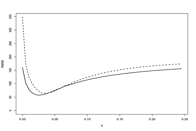
Figure 1: RMSE of Local Quadratic spectral estimation (solid) and Local Log Periodogram estimation (dashed) at frequency $0$ plotted as a function of $\delta$, based on a sample of size $n=800$ of a Gaussian ARMA(1,1) process with $\phi=.9$ and $\vartheta=.4$.

5.4 Comparison to local quadratic fitting of the log-periodogram.

It is also of interest to compare the local quadratic estimator $\tilde{f}(w)$ and the log-periodogram estimator $\bar{f}(w)$. The first 50 figures of Appendix B focus on the behavior of the new estimator as a function of $\delta$, letting this tuning parameter range over $(0,.25]$. We compare the local quadratic estimator $\tilde{f}(w)$ to the log-periodogram estimator $\bar{f}(w)$ for sample size $n=800$, for all 25 ARMA processes at both frequency $0$ and $\pi$. An example, corresponding to the ARMA process with $\phi=.9$ and $\vartheta=.4$, is seen in Figure 1. In general the log-periodogram quadratic estimator has inferior performance, although there are some values of $\delta$ for some of the processes in which the estimator $\tilde{f}(w)$ had higher RMSE. However, such cases did not occur at an optimal $\delta$, i.e., when comparing the two curves at their respective minima, the log-periodogram quadratic estimator appears to be inferior in every case. This empirical result reinforces the intuitive idea that enforcing positivity at the outset entails a constraint that may hurt performance. It is better to correct for positivity after constructing an otherwise optimal estimator; this is the case of the local quadratic estimator $\tilde{f}(w)$, as was the case of the aforementioned flat-top tapered estimators.

5.5 Simulation with non-Gaussian processes

Finally, it is important to evaluate the new methodology on non-Gaussian processes. We consider three additional simulation exercises: (i) a non-Gaussian ARMA process driven by Laplace noise, (ii) a heavy-tailed ARMA process driven by Student $t$ noise with $6$ degrees of freedom, and (iii) a polynomial Gaussian process of order two. Both the ARMA processes have the same parameter ranges as used in the Gaussian case, and the inputs are normalized so as to have variance one. The polynomial Gaussian process is a nonlinear process defined in Terdik and Meaux (1991), and is constructed by passing Gaussian white noise through a quadratic filter – see (A.1) of Appendix A. (We derive the polyspectra of this process in Proposition A.1, confirming its nonlinear properties; we also show that with a particular choice of the filter coefficients the spectral density has the form corresponding to the sum of two independent AR(1) processes, even though the process is nonlinear.) The two parameters, $\phi_{1}$ and $\phi_{2}$, that govern the dynamics of the polynomial Gaussian process are each allowed to range in the set $\{-.9,-.5,0,.5,.9\}$. The results of these simulations are provided in the tables and figures of Appendix B; since the performance of the estimators is qualitatively similar to the Gaussian case, we do not present these results in the main paper. In general, the local quadratic estimator is superior except in the case that the true process is a white noise (i.e., has a flat spectral density at the boundary).

6 Real Data Examples

We next study two data sets of current interest, U.S. Gross Domestic Product (GDP) and the Global Land-Ocean Temperature Index (GLOTI).

6.1 U.S. Gross Domestic Product

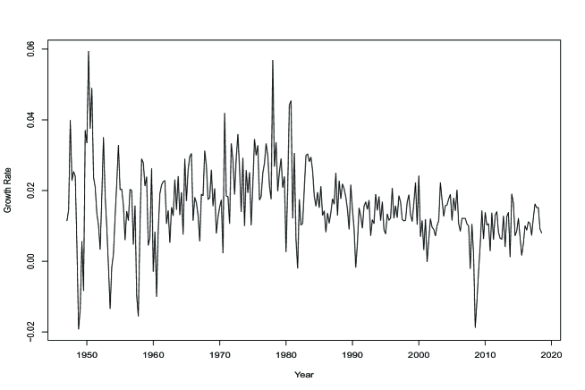
Figure 2: Growth rate of U.S. Gross Domestic Product (GDP), from 1947Q1 through 2020Q3 (units of billions of dollars, seasonally adjusted annual rate). Source: U.S. Bureau of Economic Analysis, Gross Domestic Product [GDP], retrieved from FRED, Federal Reserve Bank of St. Louis.

We consider the time series $\{Y_{t}\}$ of quarterly GDP from 1947Q1 through 2020Q3 (units of billions of dollars, seasonally adjusted annual rate). As one of the primary variables used to gauge the strength of the U.S. economy, GDP commands a tremendous interest; in particular, it is important to measure the GDP growth rate. Here we study the log differences of GDP $\{X_{t}\}$, defined via $X_{t}=\log Y_{t}-\log Y_{t-1}$ for $t=1,2,\ldots,n$, referred to as the GDP growth. This GDP growth time series exhibits features that indicate stationarity (when restricting to sub-spans of the series) is a reasonable hypothesis. In examining Figure 2 we see that the growth is sometimes negative, although in most quarters is positive; also there are possibly some cyclical effects present.

It is natural to ask whether the mean growth rate is within the typical range of growth, viz. $2\%$ to $3\%$ (see Jones (2016) for background). The answer clearly depends upon what time period is examined; GDP growth rates are somewhat lower on average after 1980, and there seems to be a further moderation beginning around 2000. We can examine the hypothesis that GDP growth over the last 20 years exceeds the lower range of the typical growth rate, viz. $2\%$; this corresponds to a one-sided test of the null hypothesis that GDP growth equals $.02$. Secondly, we can examine whether the growth exceeds the higher range of $3\%$, i.e., a one-sided test of the null hypothesis that GDP growth equals $.03$.

In order to test these hypotheses, we utilize the mean growth rate of GDP as a test statistic, restricting to the last 20 years (or $n=80$) of quarterly observations. As discussed in Section 4.1, the asymptotic variance of the sample mean of a stationary time series is $f(0)$ divided by sample size. We estimate $f(0)$ using the methods proposed in this paper, forming the $t$–statistic $\sqrt{n}\overline{x}/\sqrt{f(0)}$, and using the standard normal asymptotic critical values. More specifically, we consider both the local quadratic estimator and the log-periodogram variant, and compare the results to using the flat-top and Parzen tapers (with optimal bandwidth selection, as described in the simulation studies). Furthermore, we compare to estimates of $f(0)$ based on a fitted AR($p$) model, where $p$ is determined by minimizing the AIC criterion, and the AR-fitting method is via OLS.

The flat-top bandwidth is estimated to be $M=4$, resulting in a Parzen bandwidth of $31.82$. The data-based selection of $\delta$ for the local quadratic estimator yields $\widehat{\delta}_{*}=.245$. The AR-model method results in $\widehat{p}=2$, selected by AIC. The resulting estimates are given in Table 2. The largest estimate of $f(0)$ is given by the AR spectral estimator, followed by the log-periodogram estimator. The Parzen and local quadratic estimator give similar estimates, with the flat-top being also close.

	Parzen	Flat-top	Local quadratic	Log-periodogram	AR OLS
spectrum	0.00011185	0.00012799	0.00011534	0.00013137	0.0001815
$t$–statistic (null value $.02$)	4.34337242	4.06025137	4.27719210	4.00764423	3.4095815
$t$–statistic (null value $.03$)	2.22905000	2.08375024	2.19508579	2.05675188	1.7498218
Lower Limit	0.03127268	0.03062629	0.03112925	0.03049612	0.02873390
Upper Limit	0.04981256	0.05045895	0.04995599	0.05058912	0.05235134

Table 2: Results of analysis of GDP growth rate.

In order to test the two hypotheses, we need to divide each growth rate by 4. In the first case of $2\%$ annual growth, an upper one-sided test leads to rejection for all of the estimates of $f(0)$. In the second case of $3\%$ annual growth, the story is different: because of the higher estimate of $f(0)$ arising from the AR spectral estimator, the p-value is $.040$, indicating moderate evidence. In contrast, the p-value for the local quadratic estimator’s $t$–statistic is $0.014$, and the evidence is much more conclusive; this occurs because the relevant estimate of $f(0)$ turns out to be smaller—here is where the improved accuracy of local quadratic fitting can make a difference in practice.

We can also examine the annual growth over this period by constructing a $95\%$ confidence interval based on the asymptotic normality. Table 2 lists the lower and upper confidence limits constructed via the five different methods. Whereas the AR method allows for a growth rate as high as $5.2\%$, the local quadratic estimator indicates the growth rate is strictly less than $5\%$, but well above $3\%$.

6.2 Global Land-Ocean Temperature Index

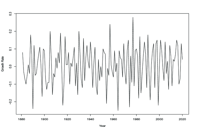
Figure 3: Growth rate of Global Land-Ocean Temperature Index (GLOTI), from 1880 through 2020. Source: NASA’s Goddard Institute for Space Studies.

We study the time series $\{Y_{t}\}$ corresponding to the GLOTI, an annual series covering the years 1880 through 2020. Climate data has received substantial attention over the past decades, and the GLOTI (in levels) shows a visually marked increase during the years following World War II. The upward trend can be assessed by examining the mean of the differenced GLOTI series, defined as $X_{t}=Y_{t}-Y_{t-1}$ for $t=1,2,\ldots,n$. This GLOTI growth series appears to have regular variation – see Figure 3 – but it is of interest to determine if the mean level changed after World War II. To address this question, consider a change point $t_{*}$ such that

$$EX_{t}=\mu_{1}1_{\{t\leq t_{*}\}}+\mu_{2}1_{\{t>t_{*}\}},$$ (25)

and that $\{X_{t}-EX_{t}\}$ is stationary; for simplicity, we will further assume that $\{X_{t}-EX_{t}\}$ is $m$-dependent (for some $m>0$).

Our null hypothesis is $H_{0}:\mu_{1}=\mu_{2}$, which is tested by comparing sample means $\overline{X}_{1}$ and $\overline{X}_{2}$ computed over samples before and after time $t_{*}$, respectively. That is, $\overline{X}_{1}$ is based on a sample of size $n_{1}$ with all times less than $t_{*}-m/2$, and $\overline{X}_{2}$ is based on a sample of size $n_{2}$ with all times greater than $t_{*}+m/2$. Then the $m$-dependence assumption ensures that $\overline{X}_{1}$ and $\overline{X}_{2}$ are independent. We can test $H_{0}$ with the statistic $\overline{X}_{1}-\overline{X}_{2}$, which has asymptotic variance (under the null) of $(n_{1}^{-1}+n_{2}^{-1})f(0)$, where $f$ is the spectral density of $\{X_{t}-EX_{t}\}$. Hence, our studentized statistic is

$$\frac{\overline{X}_{1}-\overline{X}_{2}}{\sqrt{(n_{1}^{-1}+n_{2}^{-1})\hat{f}(0)}}.$$

Estimates $\hat{f}(0)$ of $f(0)$ can be obtained using the entire sample provided the data are centered correctly; for this reason, we center the data by a mean estimate that remains consistent under $H_{a}:\mu_{1}<\mu_{2}$ (which states that growth rate has increased). This is done by estimating $\mu_{1}$ and $\mu_{2}$ via $\overline{X}_{1}$ and $\overline{X}_{2}$ respectively, and plugging these estimates in eq. (25) to get an estimate of $EX_{t}$ by which to center the data for computing sample autocovariances, etc. As in our study of GDP, we consider the local quadratic estimator and the log-periodogram variant, as well as the flat-top, Parzen, and AR($p$) estimators. In order to select the two samples, we set $t_{*}$ corresponding to the year 1950, demarcating the beginning of the post-war industrial economy after recovery from the war years. Examination of the autocorrelation plot (not shown) indicates that there is little substantial correlation past lag 2, and therefore we set $m=2$. So with $t_{*}=70$ the first sample consists of $1\leq t\leq 69$, and the second sample consists of $71\leq t\leq 140$.

	Parzen	Flat-top	Local quadratic	Log-periodogram	AR OLS
spectrum	0.00148086	0.00043289	0.00220545	0.00337354	0.00186396
$t$–statistic	-2.51529769	-4.65221263	-2.06109805	-1.66649447	-2.24196225

Table 3: Results of analysis of GLOTI growth rate.

The estimated flat-top bandwidth is $M=2m=4$, resulting in a Parzen bandwidth of $47.435$. The optimal $\widehat{\delta}_{*}$ for the local quadratic estimator is $0.02392$. The AR method results in $\widehat{p}=5$, selected by AIC. The resulting estimates are given in Table 3. The smallest estimate of $f(0)$ is given by the flat-top spectral estimator, leading to a rejection of $H_{0}$ with p-value $1.64\cdot 10^{-6}$. The Parzen, AR , and local quadratic estimators yield larger p-values of $.00595$, $.01248$, and $.01965$ respectively; they are all significant at level $0.05$. The log-periodogram variant is barely significant with p-value $.04781$. Overall there is support for the rejection of $H_{0}$ by all methods considered.

References

- [1] Andrews, D. (1991). Heteroskedasticity and autocorrelation consistent covariance matrix estimation, Econometrica, 59, 817-858.
- [2] Bartlett, M.S. (1946), On the theoretical specification of sampling properties of autocorrelated time series, J. Roy. Statist. Soc. Suppl., vol. 8, 27-41.
- [3] Bartlett, M.S. (1948). Smoothing periodograms from time series with continuous spectra, Nature, vol. 161, pp. 686-687.
- [4] Blackman, R.B. and Tukey, J.W. (1959). The Measurement of Power Spectra from the Point of View of Communications Engineering, Dover, New York.
- [5] Brillinger, D.R. (1981), Time Series: Data Analysis and Theory, Holden-Day, New York.
- [6] Brockwell, P. J. and Davis, R. A. (1991), Time Series: Theory and Methods, 2nd ed., Springer, New York.
- [7] Daniell, P.J. (1946). Discussion of paper by M.S. Bartlett. J. Roy. Statist. Soc. Suppl., vol. 8, pp. 88-90.
- [8] Fan, J. and Gijbels, I. (1996). Local polynomial modelling and its applications, Chapman and Hall/CRC Press, Boca Raton.
- [9] Fan, J. and Kreutzberger E. (1998), Automatic Local Smoothing for Spectral Density Estimation, Scan. J. Statist., vol. 25, no. 2, pp. 356-369.
- [10] Grenander, U. and Rosenblatt, M. (1957), Statistical Analysis of Stationary Time Series, Wiley, New York.
- [11] Hannan, E.J. (1970), Multiple Time Series, John Wiley, New York.
- [12] Hansen, B.E. (1992). Consistent covariance matrix estimation for dependent heterogeneous processes, Econometrica, 60, 967-972.
- [13] Jones, C.I. (2016). The facts of economic growth. In Handbook of Macroeconomics (Vol. 2, pp. 3-69). Elsevier.
- [14] Kiefer, N. and Vogelsang, T. (2002). Heteroscedastic-autocorrelation robust standard errors using the Bartlett kernel without truncation. Econometrica, 70, 2093-2095.
- [15] Kiefer, N. and Vogelsang, T. (2005). A new asymptotic theory for heteroscedasticity-autocorrelation robust tests. Econometric Theory, 21, 1130-1164.
- [16] Marron, J. S. and Ruppert, D. (1994). Transformations to reduce boundary bias in kernel density estimation, Journal of the Royal Statistical Society: Series B (Methodological), vol. 56, no. 4, pp. 653-671.
- [17] McElroy, T. and Politis, D. N. (2013). Distribution theory for the studentized mean for long, short, and negative memory time series. Journal of Econometrics, vol. 177, no. 1, pp. 60-74.
- [18] McElroy, T. S. and Politis, D. N. (2014). Spectral density and spectral distribution inference for long memory time series via fixed-b asymptotics. Journal of Econometrics, vol. 182, no. 1, pp. 211-225.
- [19] McElroy, T.S. and Politis, D.N. (2020). Time Series: A First Course with Bootstrap Starter, Chapman and Hall/CRC Press, Boca Raton.
- [20] McMurry, T. and Politis, D.N. (2015). High-dimensional autocovariance matrices and optimal linear prediction (with Discussion), Electronic Journal of Statistics, vol. 9, pp. 753-788.
- [21] Myers, R.A., Montgomery, D.C., and Anderson-Cook, C.M. (2016). Response Surface Methodology: Process and Product Optimization Using Designed Experiments (4th Edition), Wiley, New York.
- [22] Paparoditis, E. and Politis, D.N. (2012). Nonlinear spectral density estimation: thresholding the correlogram, J. Time Series Analysis, vol. 33, no. 3, pp. 386-397.
- [23] Parzen, E. (1957). On Consistent Estimates of the Spectrum of a Stationary Time Series. Ann. Math. Statist., Vol. 28, No. 2., pp. 329-348.
- [24] Parzen, E. (1961), Mathematical Considerations in the Estimation of Spectra, Technometrics, vol. 3, 167-190.
- [25] Percival, D.B. and Walden, A.T.(1993). Spectral analysis for physical applications. Multitaper and conventional univariate techniques. Cambridge University Press, Cambridge.
- [26] Politis, D.N. (2001). On nonparametric function estimation with infinite-order flat-top kernels, in Probability and Statistical Models with applications, Ch. Charalambides et al. (Eds.), Chapman and Hall/CRC Press, Boca Raton, pp. 469-483.
- [27] Politis, D.N. (2003). Adaptive bandwidth choice, J. Nonparam. Statist., vol. 15, no. 4-5, 517-533.
- [28] Politis, D.N. (2011). Higher-order accurate, positive semi-definite estimation of large-sample covariance and spectral density matrices, Econometric Theory, vol. 27, no. 4, pp. 703-744.
- [29] Politis, D.N., and Romano, J.P. (1995), Bias-corrected nonparametric spectral estimation. J. Time Ser. Anal., 16, 67–103.
- [30] Priestley, M.B. (1962), Basic considerations in the estimation of spectra, Technometrics, vol. 4, 551-564.
- [31] Priestley, M.B. (1981). Spectral Analysis and Time Series, Academic Press, New York.
- [32] Rosenblatt, M. (1984). Asymptotic normality, strong mixing and spectral density estimates, Annals Prob., 12, 1167-1180.
- [33] Rosenblatt, M. (1985), Stationary Sequences and Random Fields, Birkhäuser, Boston.
- [34] Samarov, A. (1977). Lower bound for the risk of spectral density estimates, Probl. Inform. Transm., 13, pp. 67-72.
- [35] Shao, X. and Wu, W.B. (2007). Asymptotic spectral theory for nonlinear time series. Annals Statist., Vol. 35, 1773-1801.
- [36] Taniguchi, M. and Kakizawa, Y. (2000). Asymptotic Theory of Statistical Inference for Time Series. Springer-Verlag, New York City, New York.
- [37] Terdik, G. and Meaux, L. (1991). The exact bispectra for bilinear realizable processes with Hermite degree 2, Advances in Applied Probability, Vol. 23, no. 4, pp. 798-808.
- [38] Wahba, G. (1980). Automatic smoothing of the log periodogram, J. Amer. Statist. Assoc., vol. 75, pp. 122-132.
- [39] Wu, W.B. (2005). Nonlinear system theory: another look at dependence, Proc. Nat. Acad. Sci., vol. 102, no. 40, pp. 14150–14154.
- [40] Zhou, Z. (2013). Heteroscedasticity and autocorrelation robust structural change detection, Journal of the American Statistical Association, 108(502), 726–740.
- [41] Zhou, Z. (2014). Inference of weighted -statistics for nonstationary time series and its applications, The Annals of Statistics, 42(1), 87–114.