GAS: Generating Fast and Accurate Surrogate Models for Autonomous Vehicle Systems

Abstract.

Modern autonomous vehicle systems use complex perception and control components. These components can rapidly change during development of such systems, requiring constant re-testing. Unfortunately, high-fidelity simulations of these complex systems for evaluating vehicle safety are costly. The complexity also hinders the creation of less computationally intensive surrogate models.

We present GAS, the first approach for creating surrogate models of complete (perception, control, and dynamics) autonomous vehicle systems containing complex perception and/or control components. GAS’s two-stage approach first replaces complex perception components with a perception model. Then, GAS constructs a polynomial surrogate model of the complete vehicle system using Generalized Polynomial Chaos (GPC). We demonstrate the use of these surrogate models in two applications. First, we estimate the probability that the vehicle will enter an unsafe state over time. Second, we perform global sensitivity analysis of the vehicle system with respect to its state in a previous time step. GAS’s approach also allows for reuse of the perception model when vehicle control and dynamics characteristics are altered during vehicle development, saving significant time.

We consider five scenarios concerning crop management vehicles that must not crash into adjacent crops, self driving cars that must stay within their lane, and unmanned aircraft that must avoid collision. Each of the systems in these scenarios contain a complex perception or control component. Using GAS, we generate surrogate models for these systems, and evaluate the generated models in the applications described above. GAS’s surrogate models provide an average speedup of $3.7\times$ for safe state probability estimation (minimum $2.1\times$) and $1.4\times$ for sensitivity analysis (minimum $1.3\times$), while still maintaining high accuracy.

1. Introduction

Autonomous vehicles, such as self driving cars, unmanned aircraft, and utility vehicles, are increasingly common. They navigate by perceiving the vehicle’s state (position, heading, etc.), making a control decision based on this perceived state, and moving accordingly. To preserve life and property, developers specify safety properties that the vehicle must satisfy in certain scenarios. However, 1) many sensors have a nondeterministic output (e.g., GPS and LIDAR) and 2) the vehicle’s software processes sensor values or makes decisions using complex, possibly imperfect components such as neural networks and lookup tables. Given this uncertainty in the output of the perception and control systems, proving that an autonomous vehicle will never violate safety properties in a scenario is impossible or impractical. Developers instead focus on proving that the vehicles will satisfy the safety property with high probability, using probabilistic and statistical techniques.

Monte Carlo Simulation (MCS) is perhaps the most used general method for estimating the probability of entering an unsafe state over time. However, using MCS requires a large number of resource-intensive system simulations in order to get a sufficiently accurate estimate of the vehicle state distribution over time (Menghi et al., 2020; Robert and Casella, 2004). These costs are prohibitively high, especially in development tasks that require iterative modifications or continuous re-testing of the software, including design exploration, parameter tuning, or system-software regression testing.

Surrogate Models aim to provide an accurate and faster replacement for the original costly model of many engineering systems. These models can be created using techniques such as abstraction refinement (Menghi et al., 2020), machine learning (Lin et al., 2020), or Generalized Polynomial Chaos (GPC) (Xiu, 2010). For instance, previous research has created GPC surrogate models for the equations of vehicle dynamics (Kewlani et al., 2012). However, the presence of complex perception and control components (which often dominate the original model’s execution time) hinders the application of existing surrogate model construction techniques to creating surrogate models of the complete vehicle system. For example, the output of a neural network which processes a camera image to perceive the vehicle’s state is not only affected by the ground truth state, but also multiple environmental parameters (e.g., weather, lighting, nearby objects, etc.) which may affect the neural network’s output in a nondeterministic manner. Existing techniques struggle to capture this complicated relationship between environmental parameters and the neural network output.

Our work.

We present GAS (GPC for Autonomous Vehicle Systems), the first approach for creating surrogate models of complete autonomous vehicle systems which compose complex perception and/or control components with vehicle dynamics. The resulting surrogate models are close approximations of the original vehicle models. They provide a faster alternative to MCS when developers experiment with system components, or tune various system parameters during the design and testing stages of vehicle development.

GAS first creates a perception model to calculate the distribution of error in the output of the perception system for any ground truth state. GAS directly samples this error distribution, minimizing the need for costly experimentation with environmental parameters, image generation, and neural networks. Second, GAS constructs a polynomial surrogate model of the complete vehicle system (perception, control, and dynamics) using GPC. GAS also supports systems that contain categorical variables (e.g., in the control system) using an ancillary model, overcoming a limitation of GPC. Lastly, because GAS’s perception model is created independently of downstream components, it can be reused when designers alter vehicle control and dynamics properties during development of the vehicle, potentially saving a significant amount of time.

We demonstrate the advantages of using the GAS-generated surrogate model in two applications. First, we use the surrogate model to estimate the probability that the vehicle will reach an unsafe state over time in five realistic scenarios. These scenarios model systems used in crop management vehicles, self driving cars, and unmanned aircraft, with associated safety properties. Each system uses a complex perception component (ResNet-18 or LaneNet) or a complex control component (neural network controllers or lookup tables). We show that the probability of reaching an unsafe state calculated by the surrogate model closely matches that calculated via the original model for 97% or more of time steps, while being $3.7\times$ faster on average (minimum $2.1\times$).

Second, we use the surrogate model for global sensitivity analysis of the vehicle system to initial state perturbations for the same scenarios by calculating Sobol sensitivity indices (Sobol, 2001) $1.4\times$ faster on average (minimum $1.3\times$) with an average error of 0.0004 (maximum 0.06). Lastly, we also investigate how various hyperparameters of the perception model affect GAS’s overall accuracy and speedup.

Contributions.

This paper makes several main contributions:

• Surrogate models for complex autonomous vehicle systems. We present GAS, a novel approach for using GPC to create fast and accurate surrogate models of complete autonomous vehicle systems with complex perception and control components.

• Perception models for GPC. We present models for complex perception systems that estimate the error distribution of the original systems, and use these perception models as part of our GAS approach.

• Implementation. We implement GAS as a tool which automates the creation of the perception model and the creation and usage of the GPC surrogate model. We plan to release GAS as an open-source tool in the future.

• Evaluation. We evaluate GAS on five realistic scenarios that model self driving cars, unmanned aircraft, and crop monitoring vehicles. GAS provides fast and accurate estimates of the probability that the vehicle will reach an unsafe state and the global sensitivity indices of the vehicle system.

2. Example

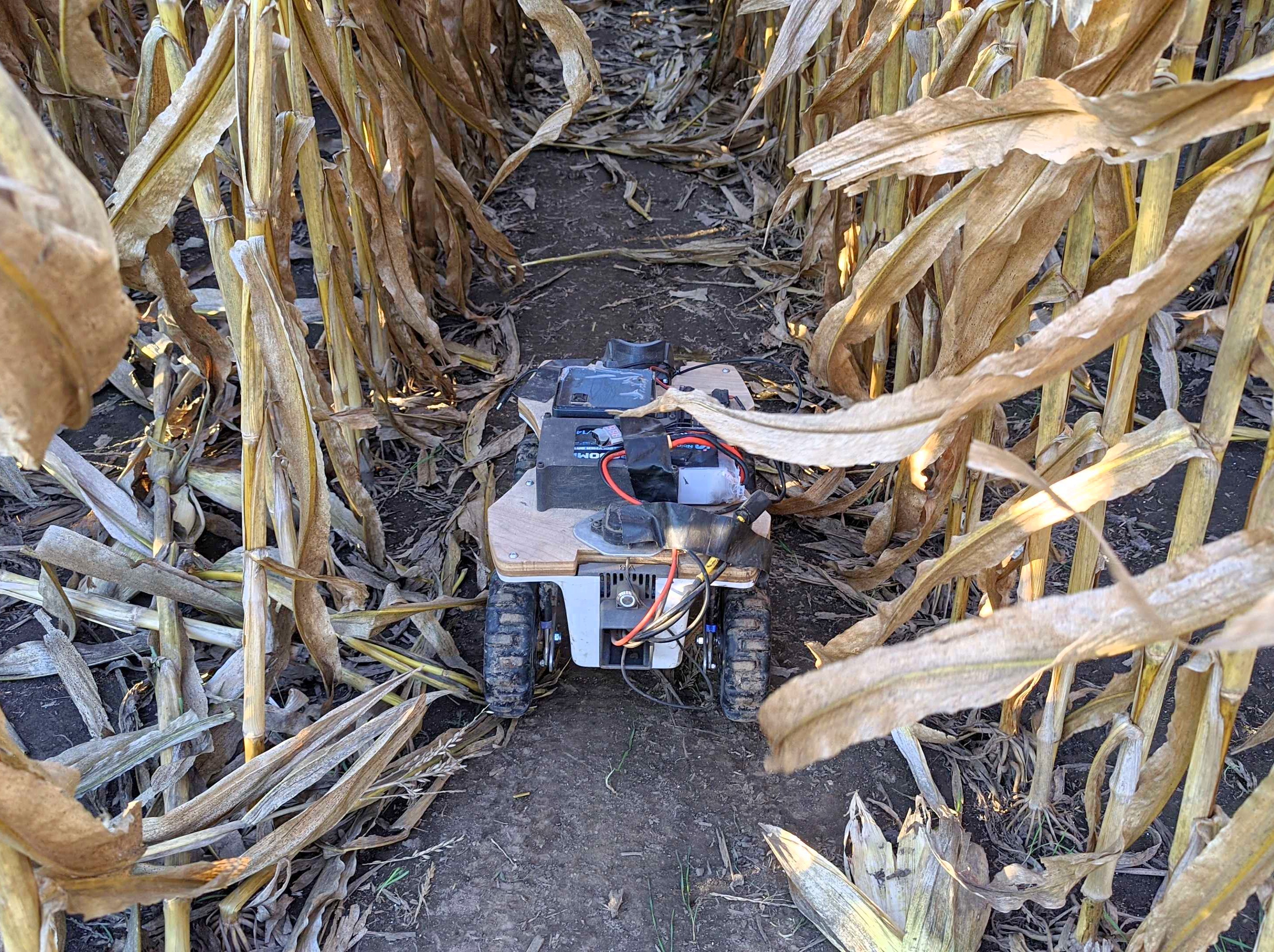
Figure 1. Real-life crop monitoring vehicle

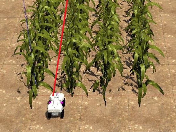
Figure 2. Gazebo simulation – overhead view

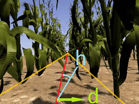
Figure 3. Gazebo simulation – front camera view

Consider an autonomous vehicle which travels between two rows of crops in order to monitor crop growth and detect weeds. Farmers use this information to adjust fertilizer and herbicide levels for each location. We have adapted this scenario from (Sivakumar et al., 2021). Figures 3-3 illustrate the scenario. The desired path is shown in red.

The top half of Figure 4 shows a block diagram representation of the system model $M_{V}$ responsible for driving the vehicle between two rows of crops. First, a camera captures the area in front of the vehicle. The image depends on the current vehicle state as well as environmental conditions. Environmental variables include crop types, crop growth stage, crop model, and lighting conditions. Together, these variables comprise the environment state space $\mathbb{D}_{E}$. The neural network analyzes the image to perceive the current vehicle state. It is a regression neural network, producing a single state prediction. The relevant state variables in this scenario are: 1) The heading angle $h$, which is the angle between the vehicle’s current heading and the imaginary centerline between the two rows of crops; $h$ can take values in $[-\pi,\pi]$ radians, with $0$ corresponding to the direction of the centerline. 2) The distance $d$ of the vehicle from the centerline; $d$ can take values in $[-0.38,0.38]$ meters, with $0$ corresponding to the centerline. The vehicle state space is therefore $\mathbb{D}_{S}=[-\pi,\pi]_{h}\times[-0.38,0.38]_{d}$.

As neural networks are inherently approximate, the state perceived by the neural network may not be the same as the ground truth. The vehicle uses this approximate heading and distance reading to calculate a steering angle in order to keep the vehicle on the centerline. Finally, the vehicle moves according to its constant speed and commanded steering angle.

Unsafe states.

We wish to avoid two undesirable outcomes: 1) if $|d|>0.228m$, the vehicle will hit the crop stems, and 2) if $|h|>\pi/6$, the neural network output becomes highly inaccurate and recovery may be impossible. To avoid these outcomes, we want the vehicle to remain in the safe region, defined as all states within $\mathbb{D}_{S}^{\textit{safe}}=[-\pi/6,\pi/6]_{h}\times[-0.228,0.228]_{d}$. Because the vehicle makes steering decisions based on approximate data, we cannot be certain that the vehicle will remain safe. Instead, we answer the question: What is the probability that the vehicle will remain safe over a period of time?

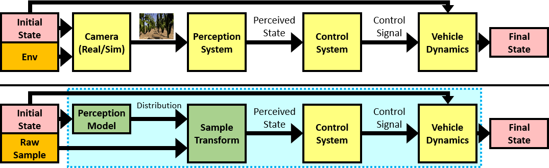
Figure 4. Crop monitor vehicle model: original (top) and abstract (bottom). GAS replaces the outlined section with a surrogate model.

Monte Carlo Simulation.

In Monte Carlo Simulation (MCS), we simulate the vehicle’s movement a large number of times and count the number of times the vehicle reaches an unsafe state. We use Gazebo (Figures 3 and 3) for precise control over the simulation environment.

We simulate 1,000 samples over 100 time steps of 0.1 seconds each. We randomly sample environmental conditions from an environment distribution $\mathcal{D}_{E}$ that contains two types of crops, four crop growth stages, crop model variations, and a range of lighting conditions. We also choose the initial vehicle state from a normal distribution. For each sample at each time step, we invoke the autonomous vehicle model, which 1) captures an image from an expensive Gazebo simulation in the current vehicle state and environment, 2) passes the image through the neural network to get the approximate perceived state, 3) calculates a steering angle based on the perceived state, and 4) calculates the position of the vehicle after one time step using the actual state and steering angle. At each time step, we count how many samples are still in a safe state.

2.1. GAS: Using Generalized Polynomial Chaos

We present GAS, a novel approach for creating surrogate models of complex vehicle systems using Generalized Polynomial Chaos (GPC). While previous research (e.g., (Kewlani et al., 2012)) has explored using GPC to create models of vehicle dynamics, this is insufficient in our scenario as the process of capturing and processing the image contributes to over 99% of the simulation time. GAS aims to instead use GPC to create a surrogate for the entire vehicle model – perception, control, and dynamics.

Perception model construction.

The output of the vehicle’s perception neural network depends on the image captured by the front camera. This image depends not only on the vehicle’s state, but also environmental parameters (e.g., lighting, crop type, crop age, etc.). Given a distribution of environmental parameters, there is a corresponding output distribution of the perception neural network for each ground truth state. Figure 5 shows the error distribution of the ResNet-18 networks used by this vehicle on the original validation dataset of real-world images collected by the vehicle’s camera in a cornfield. The histogram shows the actual error frequency, while the line shows the fitted normal distribution. The distribution closely matches the histogram, indicating that the error of the neural network is normally distributed.

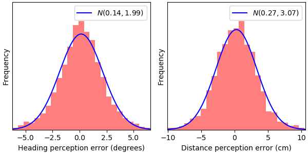
Figure 5. Error distribution of the neural network for the validation set of real-world images.

GAS must sample this output distribution when creating the GPC model. However, 1) the environmental parameters have a smaller effect on the perceived state as compared to the vehicle’s actual state, and 2) directly using the numerous environmental parameters increases the input space over which GAS must construct the GPC model, which increases model construction time. GAS therefore abstracts away the actual environmental parameters by creating a perception model. GAS does not require the perception model to be a perfect abstraction of the neural network. Instead, GAS trains the perception model by selecting an $11\times 11$ grid $G$ of ground truth states in the safe region. At each grid point $(h,d)$, it randomly samples images from $\mathcal{D}_{E}$, and records the neural network outputs. It calculates the mean $\mu(h,d)$ and covariance $\sigma^{2}(h,d)$ of the outputs at each state. GAS trains a degree 4 polynomial regression model $M_{\mathit{per}}$ to predict each component of $\mu$ and $\sigma^{2}$ at any safe state. Figure 6 visually compares the neural network output distribution to the distribution predicted by $M_{\mathit{per}}$ for images captured within Gazebo. The red dashed ellipse and the blue solid ellipse show the $3\sigma$ confidence boundaries for the neural network output distribution and the distribution predicted by the perception model, respectively. The two distributions closely match each other, especially when the vehicle is near the center and pointing straight ahead.

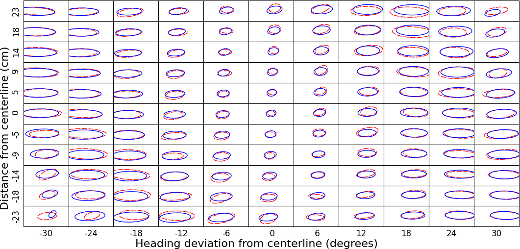
Figure 6. Comparison of neural network output distribution (dashed red ellipse) to distribution predicted by perception model (solid blue ellipse). Each box represents a distinct ground truth state used to construct the perception model. The X and Y-Axes vary the ground truth heading and distance, respectively.

GPC Surrogate model construction.

Next, GAS creates an abstract vehicle model $M^{\prime}_{V}$, shown in the bottom half of Figure 4. $M^{\prime}_{V}$ first uses the perception model to obtain the neural network output distribution in the current state. Second, it transforms a sample from a 2D standard normal distribution into a sample from this output distribution by multiplying by $\sigma$ and adding $\mu$. The rest of the vehicle model uses this transformed sample as the perceived state. GAS now uses GPC to create a polynomial model of the complete system (outlined section of Figure 4). This model $M_{\mathit{GPC}}$ is a $4^{th}$ degree polynomial over 4 variables (2 state variables and a 2D normal distribution sample) with 70 terms, including 53 interaction terms. GAS replaces the original model in the MCS procedure outlined above with this surrogate model to estimate the state distribution of the vehicle over time. GAS also increases the number of samples for distribution estimation to 10,000 for $M_{\mathit{GPC}}$ in order to decrease sampling error.

2.2. Results

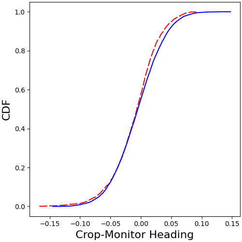
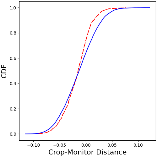
Figure 7. State distribution at the final time step: heading (left) and distance from the centerline (right)

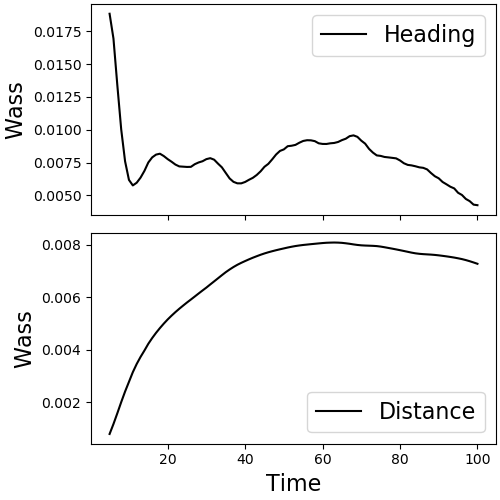
Figure 8. Wasserstein metric (distribution similarity) over time steps

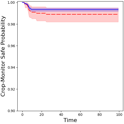
Figure 9. Probability of remaining in a safe state over time steps

Accuracy.

Figure 9 shows a comparison of the heading and distance distributions after 100 time steps. The X Axis shows the variable value and the Y Axis shows the cumulative probability. The blue solid and red dashed plots show the distributions estimated using MCS and GAS, respectively. We compare the GAS and MCS distributions using the Kolmogorov-Smirnov (KS) statistic and the Wasserstein metric. Figure 9 shows how the Wasserstein metric evolves over time. The X Axis shows time steps and the Y Axis shows the Wasserstein metric. The low Wasserstein metric value indicates good correlation between the two distributions at all times. The KS statistic also remains below 0.14. Figure 9 shows the probability of remaining in a safe state over time. The X Axis shows time steps and the Y Axis shows the probability of remaining safe. The shaded regions show the 95% bootstrap confidence interval. Around each plot, the bootstrap confidence interval indicates the variation that can occur as a result of sampling error. As GAS evaluates $M_{\mathit{GPC}}$ for $10\times$ more samples than $M_{V}$, its confidence interval is smaller. We use the t-test to check if the safe state probabilities are similar: it passes for 99 of 100 time steps, indicating high similarity.

Time.

GAS is 2.3x faster than MCS on our hardware. MCS required 19.5 hours. Gathering the training data for the perception model required 8.5 hours. The time required for training the perception model, constructing the polynomial approximation with GPC, and using the GPC approximation was negligible in comparison ($<1$ minute). Increasing the number of samples or the number of time steps would further increase the gap between the two methods, since the time required to construct the perception model is a one-time cost.

3. Background

We present key definitions pertaining to GPC. Dedicated books (e.g., (Xiu, 2010)), provide more details.

Orthogonal polynomials.

Assume $X$ is a continuous variable with support $S_{X}$ and probability density $p_{X}:S_{X}\rightarrow\mathbb{R}$. Let $\Psi=\{\Psi_{n}|n\in\mathbb{N}\}$ be a set of polynomials, where $\Psi_{n}$ is an $n^{th}$ degree polynomial. Then $\Psi$ is a set of orthogonal polynomials with respect to $X$ if for all $n\neq m$, $\int_{S_{X}}\Psi_{n}(x)\Psi_{m}(x)p_{X}(x)dx=0$. The orthogonal polynomial $\Psi_{n}$ has $n$ distinct roots in $S_{X}$.

Orthogonal polynomials exist for several probability distributions. For example, the Legendre, Hermite, Jacobi, and Laguerre polynomials are orthogonal for the uniform, normal, beta, and gamma distributions respectively.

Orthogonal polynomial projection (GPC).

Let $f:S_{X}\rightarrow\mathbb{R}$. Then the $N^{th}$ order orthogonal polynomial projection of $f$, written as $f_{N}$, with respect to a set of orthogonal polynomials $\Psi$, is:

(1) $$f_{N}=\sum\limits_{i=0}^{N}c_{i}\Psi_{i}\quad\text{where}\quad c_{i}=\frac{\int_{S_{X}}f(x)\Psi_{i}(x)p_{X}(x)dx}{\int_{S_{X}}\Psi_{i}^{2}(x)p_{X}(x)dx}$$

If $f$ is an $N^{th}$ degree polynomial, then $f_{N}=f$. Otherwise, $f_{N}$ is the optimal $N^{th}$ degree polynomial approximation of $f$ w.r.t. $X$, in the sense that it minimizes $\ell_{2}$ error, which is calculated as $\int_{S_{X}}(f(x)-f_{N}(x))^{2}p_{X}(x)dx$. As $N\rightarrow\infty$, the $\ell_{2}$ error approaches 0, that is, we can construct arbitrarily good approximations of $f$. $f_{N}$ is called the $N^{th}$-order generalized polynomial chaos (GPC) approximation.

Lagrange basis polynomials.

Given $N$ points $(x_{i},y_{i}),\ 1\leq i\leq N$, where all $x_{i}$ are distinct, Equation 2 shows the Lagrange basis polynomials $L_{i}$ for each $i$.

(2) $$L_{i}(x)=\prod\limits_{\begin{subarray}{c}1\leq j\leq N\\ j\neq i\end{subarray}}\frac{x-x_{j}}{x_{i}-x_{j}}$$

Gaussian quadrature.

To use Equation 1, we must perform multiple integrations to calculate the coefficients $c_{i}$ ($i\in\{0\ldots N\}$). For any non-trivial function $g$, we must use numerical integration by approximating the integral with the following sum:

(3) $$\int\limits_{S_{X}}g(x)p_{X}(x)dx\approx\sum\limits_{i=1}^{N}w_{i}g(x_{i})\ \ \text{where}\ \ w_{i}=\int\limits_{S_{X}}L_{i}(x)p_{X}(x)dx$$

We choose $w_{i}$ and $x_{i}$ so as to minimize integration error. In Gaussian quadrature, we choose $x_{i}$ to be the $N$ roots of $\Psi_{N}$, the $N^{th}$ order orthogonal polynomial w.r.t. $X$. We calculate the corresponding weights using the Lagrange basis polynomials $L_{i}$ (Equation 2) passing through $x_{j}\ \forall j\neq i$.

Multivariate GPC.

GPC can be easily extended to the multivariate case, as long as all all random variables are independent. Let $\mathbf{X}=(X_{1},\ldots,X_{d})$ be the $d$ independent random variables (not necessarily following the same distribution) and let $f$ be a function over $\mathbf{X}$. The orthogonal polynomials $\mathbf{\Psi_{i}}$ for $\mathbf{X}$ are simply the products of the orthogonal polynomials $\Psi_{i_{1}},\ldots,\Psi_{i_{d}}$ for $X_{1},\ldots,X_{d}$ respectively. The GPC approximation closely resembles the one for the univariate case:

(4) $$f_{N}=\sum\limits_{\mathbf{i}}c_{\mathbf{i}}\mathbf{\Psi_{i}}\quad\text{where}\quad c_{\mathbf{i}}=\frac{\int_{S_{\mathbf{X}}}f(\textbf{\em{x}}{})\mathbf{\Psi_{i}}(\textbf{\em{x}}{})p_{\mathbf{X}}(\textbf{\em{x}}{})d\textbf{\em{x}}{}}{\int_{S_{\mathbf{X}}}\mathbf{\Psi_{i}}^{2}(\textbf{\em{x}}{})p_{\mathbf{X}}(\textbf{\em{x}}{})d\textbf{\em{x}}{}}$$

We calculate $c_{\mathbf{i}}$ using a variant of Equation 3 in which we sum over all dimensions of $\mathbf{i}$.

Global sensitivity (Sobol) indices.

Sobol indices (Sobol, 2001) decompose the variance of the model output over the entire input distribution into portions that depend on subsets of the input variables $X_{i}$. The first order sensitivity indices show the contribution of a single input variable to the output variance. For a variable $X_{i}$, the sensitivity index is $S_{i}=V_{i}/V$. Here, $V=\mathit{Var}_{\mathit{\mathbf{X}}}(f(\textbf{\em{x}}{}))$ is the total variance and

(5) $$V_{i} =\mathit{Var}_{X_{i}}(E_{\mathit{\mathbf{X}_{\neg i}}}(f(\textbf{\em{x}}{})|X_{i}=x_{i}))$$

$$\text{where}\quad\mathit{\mathbf{X}_{\neg i}} =\{X_{1},\ldots,X_{d}\}\setminus\{X_{i}\}$$

We can evaluate Equation 5 analytically when $f$ is a polynomial (such as those generated via GPC) and when it is possible to calculate the moments of each independent component of $\mathbf{X}$ analytically. For more complex functions and distributions, it becomes necessary to estimate Equation 5 empirically using Monte Carlo estimators (Sobol, 2001, Equation 6).

4. GAS Approach

We present the GAS approach for creating a polynomial surrogate model of complex autonomous vehicle systems. GAS consists of three high level steps:

1. Create a deterministic complete vehicle model.

2. Train a perception model and use it to replace the regression neural network used for state perception in the vehicle model (Algorithms 1-2).

3. Construct a GPC surrogate model from the vehicle model (Algorithm 3).

GAS automates almost the entire process of constructing and using the surrogate model. The user provides the perception model training data, the distributions of state and random variables, GPC order, and simulation parameters. GAS infers the optimal degree of polynomial regression for the perception model using cross-validation to maximize accuracy while preventing overfitting. We plan to release GAS as open-source software in the future.

4.1. Creating a deterministic vehicle model

First, we represent the complete vehicle model as a function of independent random variables, $M_{V}:\mathbb{D}_{S}\times\mathbb{D}_{E}\times\mathbb{D}_{R}\rightarrow\mathbb{D}_{S}$. $S\in\mathbb{D}_{S}$ is a vector of state variables (e.g., position and rotation), $E\in\mathbb{D}_{E}$ is a vector of environment-related random variables that affect the neural network (e.g., weather and lighting conditions that affect the image processed by the neural network), and $R\in\mathbb{D}_{R}$ is a vector of random variables that do not affect the neural network, but affect other parts of $M_{V}$. Making $M_{V}$ deterministic is necessary as GPC produces a deterministic polynomial model over independent random variables. Because multivariate GPC requires the input variables to be independent, we remove any input variable dependencies by isolating their independent components and using those as the input variables instead.

For the example in Section 2, $\mathbb{D}_{S}$ is the Cartesian product of the range of the heading and distance variables, $\mathbb{D}_{E}$ has variables that control crop type, crop age, and lighting, and $\mathbb{D}_{R}$ is unused. The top half of Figure 4 describes $M_{V}$.

4.2. Replacing the perception system

The output of regression neural networks which use camera images to perceive the vehicle’s state is affected by environmental factors unrelated to the vehicle’s state. For a given ground truth state, such perception systems produce a distribution of possible perceived states. To enable faster sampling of this output distribution, GAS replaces the perception system with a perception model prior to constructing the GPC polynomial model. Algorithm 1 shows how GAS creates the perception model. The steps are as follows:

1. Let $\mathbb{D}_{S}^{\textit{safe}}$ be the set of safe states. We pick a set of ground truth states $G\subset\mathbb{D}_{S}^{\textit{safe}}$, such that $G$ is an evenly spaced tensor grid that includes the extreme states within $\mathbb{D}_{S}^{\textit{safe}}$.

2. For each $g\in G$, GAS captures a list of images $I_{g}$ using a photo-realistic simulator such as Gazebo (Koenig and Howard, 2004) or CARLA (Dosovitskiy et al., 2017). For each image, GAS randomly samples $E$ from the environment distribution $\mathcal{D}_{E}$ ($E\sim\mathcal{D}_{E}$). GAS obtains a large number of images per state ($N_{i}\geq 350$) to get a high confidence estimate of the output distributions in the next step.

3. For each $g\in G$, GAS passes $I_{g}$ through the neural network to obtain a list of network outputs $O_{g}$. GAS calculates the mean $\mu_{g}$ and covariance $\sigma^{2}_{g}$ of $O_{g}$.

4. GAS trains a polynomial regression model $M_{\mathit{per}}$ to predict the components of $\mu_{S}$ and $\sigma_{S}^{2}$ given $S\in\mathbb{D}_{S}^{\textit{safe}}$.

$M_{\mathit{per}}$ returns the distribution parameters $(\mu_{S},\sigma_{S}^{2})$ of possible outputs. We create an abstracted vehicle model $M^{\prime}_{V}:\mathbb{D}_{S}\times\mathbb{R}^{n}\times\mathbb{D}_{R}\rightarrow\mathbb{D}_{S}$ (Algorithm 2) to use $M_{\mathit{per}}$ instead of the neural network. Instead of a sample from $\mathcal{D}_{E}$, $M^{\prime}_{V}$ accepts a sample $N$ from a multivariate standard normal distribution $\mathcal{N}(0,1)$. It calculates $\mu_{S}$ and $\sigma_{S}^{2}$ using $M_{\mathit{per}}$, and transforms $N$ to a sample from $\mathcal{N}(\mu_{S},\sigma_{S})$. $M^{\prime}_{V}$ uses this sample as the perceived state for the rest of the model consisting of the vehicle’s control and dynamics systems.

For the example in Section 2, $\mathbb{D}_{S}^{\textit{safe}}$ is the Cartesian product of the safe range of the heading and distance variables, $G$ is an $11\times 11$ grid within $\mathbb{D}_{S}^{\textit{safe}}$, and $M_{\mathit{per}}$ is a degree 4 polynomial regression model that predicts the five parameters of the distribution of the perceived state (mean heading and distance, heading and distance variance, and correlation). The bottom half of Figure 4 describes $M^{\prime}_{V}$. As there are two state variables, the raw sample is drawn from a 2D standard distribution.

1:Input $G$: set of ground truth states; $\mathcal{D}_{E}$: distribution of environment variables; $N_{i}$: number of images to capture for each $g\in G$

2:Returns $M_{\mathit{per}}$: trained perception model; $d_{\mathit{per}}$: polynomial degree of perception model

3:function TrainPerceptionModel($G,\mathcal{D}_{E},N_{i}$)

4:    $\mathit{TrainTestData}\leftarrow\{\;\}$

5:    for $g\in G$ do

6:         $I_{g}\leftarrow[\;]$

7:         for $i$ from $1$ to $N_{i}$ do

8:             $E\sim\mathcal{D}_{E}$

9:             $\mathit{Img}\leftarrow\textsc{CaptureImage}(g,E)$

10:             $I_{g}\leftarrow I_{g}::\mathit{Img}$          

11:         $O_{g}\leftarrow\textsc{NeuralNetwork}(I_{g})$

12:         $\mu_{g}\leftarrow\textsc{Mean}(O_{g})$

13:         $\sigma^{2}_{g}\leftarrow\textsc{Covariance}(O_{g})$

14:         $\mathit{TrainTestData}\leftarrow\mathit{TrainTestData}[g\mapsto(\mu_{g},\sigma^{2}_{g})]$     

15:    $M_{\mathit{per}},d_{\mathit{per}}\leftarrow\textsc{PolyRegressionModel}(\mathit{TrainTestData})$

Algorithm 1 Training the perception model

1:Input $S$: initial state of vehicle; $N$: raw sample to be transformed into neural network output sample; $R$: other random variables; $M_{\mathit{per}}$: trained perception model

2:Returns $S^{\prime}$: state of vehicle after one time step

3:function $M^{\prime}_{V}$($S,N,R,M_{\mathit{per}}$)

4:    $\mu_{S},\sigma^{2}_{S}\leftarrow M_{\mathit{per}}(S)$

5:    $O_{S}\leftarrow\textsc{Transform}(N,\mu_{S},\sigma^{2}_{S})$

6:    $S^{\prime}\leftarrow\textsc{VehicleControlAndDynamics}(S,O_{S},R)$

Algorithm 2 Abstracted vehicle model

We assume the output is distributed according to $\mathcal{N}(\mu_{S},\sigma_{S})$ as we can easily define the distribution in terms of $\mu_{S},\sigma_{S}^{2}$. We have observed that, for real-world input images, the output distribution of perception neural networks indeed tends to be normally distributed (Figure 5). However, we can use the same method for other distributions if 1) the parameters of the fitted distribution vary smoothly as the ground truth changes, and 2) orthogonal polynomials corresponding to that distribution exist for use with GPC (e.g., the uniform and beta distributions).

4.3. GPC for the complete vehicle system

Algorithm 3 shows how GAS constructs the GPC approximation of the abstracted vehicle model:

1. GAS constructs a joint distribution $J$ over $\mathbb{D}_{S}\times\mathbb{R}^{n}\times\mathbb{D}_{R}$. For the state variables, GAS chooses a normal or truncated normal distribution $\mathcal{D}_{S}^{\textit{safe}}$ over the safe state space $\mathbb{D}_{S}^{\textit{safe}}$. GAS uses $\mathcal{N}(0,1)$ for the perception model raw sample. For the other random variables, GAS uses their actual distribution $\mathcal{D}_{R}$.

2. GAS constructs the basis polynomials which are orthogonal w.r.t. $J$. Increasing the order $o_{\mathit{gpc}}$ increases accuracy, but also runtime.

3. GAS chooses Gaussian quadrature nodes for $J$ and calculates the corresponding weights using Equation 3.

4. GAS evaluates the abstracted model $M^{\prime}_{V}$ at the chosen samples.

5. GAS calculates the GPC polynomial model as the weighted sum of the orthogonal polynomials using Equation 1.

For the example in Section 2, $J=\mathcal{N}(0,\pi/18)\times\mathcal{N}(0,0.076)\times\mathcal{N}(0,1)^{2}$. Specifically, for the state variables, we choose normal distributions such that the edge of the safe state space lies at the $3\sigma$ boundary. $\Psi$ is a set of 70 multivariate Hermite polynomials (the orthogonal polynomials for normal distributions). These polynomials are formed by taking the product of the Hermite polynomials for each variable in $J$, such that the total order is at most 4. $X$ and $W$ are a set of 624 quadrature nodes and the corresponding weights. Lastly, $M_{\mathit{GPC}}$ is an order 4 polynomial over the variables in $J$.

1:Input $\mathcal{D}_{S}^{\textit{safe}}$: distribution over $\mathbb{D}_{S}^{\textit{safe}}$; $\mathcal{D}_{R}$: distribution of other random variables; $o_{\mathit{gpc}}$: order of GPC model; $M^{\prime}_{V}$: abstracted vehicle model

2:Returns $M_{\mathit{GPC}}$: GAS surrogate model

3:function CreateGPCModel($\mathcal{D}_{S}^{\textit{safe}},\mathcal{D}_{R},o_{\mathit{gpc}},M^{\prime}_{V}$)

4:    $J\leftarrow\textsc{Join}(\mathcal{D}_{S}^{\textit{safe}},\mathcal{N}(0,1),\mathcal{D}_{R})$

5:    $\Psi\leftarrow\textsc{GenerateOrthogonalPolynomials}(o_{\mathit{gpc}},J)$

6:    $X,W\leftarrow\textsc{GenerateQuadNodesAndWeights}(o_{\mathit{gpc}},J)$

7:    $Y\leftarrow[M^{\prime}_{V}(x)$ for $x\in X]$

8:    $M_{\mathit{GPC}}\leftarrow\textsc{QuadratureAndGPC}(\Psi,X,W,Y)$

Algorithm 3 GAS surrogate model construction

Categorical state variables.

Some vehicle models have categorical state variables. For example, many control systems operate in multiple modes. The control system can switch modes if certain conditions are met, and the current mode affects the control decisions. In this case, the current mode is a categorical state variable.

Unlike categorical variables, polynomial inputs and outputs are continuous intervals. Therefore, we cannot use GPC for predicting categorical variables, or accept a categorical variable as an input to the GPC model. GAS solves this problem by using multiple GPC sub-models and using a separate classifier for predicting categorical variables. This procedure is known as multi-element GPC (ME-GPC).

Consider a vehicle model $M_{V}$ whose state includes a categorical variable $X$ with the domain $\mathbb{D}_{X}=\{x_{1},\ldots,x_{k}\}$. GAS uses GPC to create a separate polynomial model for each $x_{i}\in\mathbb{D}_{X}$. The compound surrogate model chooses which of these sub-models to use based on the current vehicle state. In this way, GAS calculates all output state variables except $X$. For predicting $X$, GAS creates an ancillary classifier, which it trains as follows:

1. GAS picks a set of states $G$ from the safe states $\mathbb{D}_{S}^{\textit{safe}}$, such that $G$ is an evenly spaced tensor grid that includes the most extreme states within $\mathbb{D}_{S}^{\textit{safe}}$, and includes all categorical values in $\mathbb{D}_{X}$.

2. For each $g\in G$, GAS evaluates $M_{V}(g,E,R)$ for a large number of samples ($\geq 350$) of $E$ and $R$. GAS isolates the value of $X$ in the output and determines the most frequent value $X_{\mathit{mode}}$.

3. GAS trains a classifier to predict $X_{\mathit{mode}}$ for any $S\in\mathbb{D}_{S}^{\textit{safe}}$.

GAS returns the value $X_{\mathit{mode}}$ predicted by the classifier as the value of $X$ in the output. This method can be generalized to multiple categorical variables, but the number of separate GPC approximations required can become impractical.

4.4. Applications of the GAS surrogate model

Calculating probability of remaining in a safe state over time.

GAS uses the surrogate model to estimate the probability that the vehicle will remain in a safe state over time (Algorithm 4). GAS creates initial joint samples using the initial state distribution, the raw sample distribution, and the distribution of other random variables. At each time step, GAS evaluates the surrogate model on each joint sample to get the next state. If the next state is safe, GAS chooses new random values to prepare the joint sample for the next time step. Finally, GAS calculates and logs the fraction of samples that are still in the safe region.

1:Input $N_{s}$: number of samples to use for distribution estimation; $T$: number of time steps; $\mathcal{D}_{S}^{0}$: initial state distribution; $\mathcal{D}_{R}$: distribution of other random variables; $\mathit{Pred}$: safety predicate; $M_{\mathit{GPC}}$: constructed GAS surrogate model

2:Returns $P_{\mathit{safe}}$: probability that the vehicle is safe until each time step

3:function EstimateSafeProb($N_{s},T,\mathcal{D}_{S}^{0},\mathcal{D}_{R},\mathit{Pred},M_{\mathit{GPC}}$)

4:    $X\leftarrow[\;]$; $P_{\mathit{safe}}\leftarrow\{\;\}$

5:    for $i$ from $1$ to $N_{s}$ do

6:         $x\sim\textsc{Join}(\mathcal{D}_{S}^{0},\mathcal{N}(0,1),\mathcal{D}_{R})$

7:         $X\leftarrow X::x$     

8:    for $t$ from $1$ to $T$ do

9:         $X^{\prime}\leftarrow[\;]$

10:         for $x\in X$ do

11:             $S^{\prime}\leftarrow M_{\mathit{GPC}}(x)$

12:             if $\textsc{Safe}(S^{\prime},\mathit{Pred})$ then

13:                 $N^{\prime}\sim\mathcal{N}(0,1)$

14:                 $R^{\prime}\sim\mathcal{D}_{R}$

15:                 $X^{\prime}\leftarrow X^{\prime}::(S^{\prime},N^{\prime},R^{\prime})$                       

16:         $X\leftarrow X^{\prime}$

17:         $P_{\mathit{safe}}\leftarrow P_{\mathit{safe}}[t\mapsto|X|/N_{s}]$     

Algorithm 4 Estimating the probability of remaining in a safe state over time

1:Input $N_{s}$: number of samples to use for sensitivity estimation; $i$: index of state variable to calculate sensitivity for; $\mathcal{D}_{S}$: current state distribution; $\mathcal{D}_{R}$: distribution of other random variables; $M$: model ($M_{\mathit{GPC}}$ or $M^{\prime}_{V}$)

2:Returns $S_{i}$: sensitivity index of selected state variable

3:function EstimateSensitivity($N_{s},i,\mathcal{D}_{S},\mathcal{D}_{R},M$)

4:    $Y_{0}\leftarrow[\;]$; $Y_{1}\leftarrow[\;]$

5:    for $i$ from $1$ to $N_{s}$ do

6:         $x_{0},x_{1}\sim\textsc{Join}(\mathcal{D}_{S},\mathcal{N}(0,1),\mathcal{D}_{R})$

7:         $y_{0}\leftarrow M(x_{0})$; $y_{1}\leftarrow M(x_{1}[i\mapsto x_{0}[i]])$

8:         $Y_{0}\leftarrow Y_{0}::y_{0}$; $Y_{1}\leftarrow Y_{1}::y_{1}$     

9:    $S_{i}\leftarrow(\textsc{Mean}(Y_{0}*Y_{1})-\textsc{Mean}(Y_{0})^{2})/\textsc{Var}(Y_{0})$

Algorithm 5 Using estimators to calculate sensitivity indices

Computing Sobol indices.

GAS uses $M_{\mathit{GPC}}$ to calculate Sobol sensitivity indices in two ways. In the analytical approach, GAS calculates sensitivity indices by first calculating conditional expected values as polynomials and then calculating their variance (Equation 5). In the empirical approach, GAS instead uses Monte Carlo estimators ((Sobol, 2001, Equation 6) as implemented in Algorithm 5).

While the analytical approach precisely calculates sensitivity indices, it is relatively slow as GAS must calculate expected values as a function of the variable whose sensitivity is being calculated. The empirical approach becomes more accurate as the number of samples increases. Despite this, it can be faster than the first approach due to the speed of evaluating $M_{\mathit{GPC}}$.

Rapid iteration.

During development of an autonomous vehicle system, the vehicle model can change rapidly as the perception neural network or vehicle control parameters are tweaked. GAS enables faster testing of these prototypes thanks to its compositional approach. If the same perception system is used while changing the control and dynamics, then GAS saves time by reusing the existing perception model. If the perception system is changed, GAS must rerun Algorithms 1-3, but if doing so is faster than using MCS, the time saved adds up with each iterative change.

4.5. Properties of the GAS approach

Accuracy.

Multiple GAS parameters affect the accuracy of the GPC model: the size of the tensor grid $|G|$, the number of images taken for each grid point $N_{i}$, the degree of polynomial regression used for the perception model, and the GPC order $o_{\mathit{gpc}}$. Under certain conditions, GAS converges in distribution to the exact solutions.

Lemma 0 (Perception Model Convergence).

Assume that 1) for the given environment distribution $\mathcal{D}_{E}$, the distribution of the outputs of a perception neural network $\mathcal{N}$ in any ground truth state $S$ is Gaussian over the perceived state, and 2) each component of the distribution parameters $(\mu_{S},\sigma_{S}^{2})$ is an analytic function of $S$. Then, the output distribution of the perception model $M_{\mathit{per}}$ in any state approaches $\mathcal{N}$’s output distribution at that state as $|G|$, $N_{i}$, and $d_{\mathit{per}}$ increase.

Proof Sketch.

Increasing $|G|$ increases the number of ground truth states used to train the perception model. Increasing $N_{i}$ increases the accuracy of $\mathcal{N}$’s output distribution parameters calculated at each $S$. Since these distribution parameters are analytic functions of $S$, they can be calculated using a Taylor series over $S$. After increasing the number and accuracy of training data points, the accuracy of the perception model can be arbitrarily increased by increasing $d_{\mathit{per}}$. ∎

We use standard statistical tests such as the Shapiro-Wilk test to check if $\mathcal{N}$’s outputs have a Gaussian distribution for the environment distribution $\mathcal{D}_{E}$ used in Section 4.2. We have observed this to be true in practice (Figure 5). We can also use a different base distribution (and corresponding orthogonal polynomials for GPC) if fits the data better across the state space.

Practically, controlling the error of the perception model (or any approximation of a neural network) is an open problem (Cheng et al., 2019; Pan and Rajan, 2020). Precise analytic calculation of the perception model error is intractable, but we can empirically estimate the error.

Lemma 0 (GPC Error Bound).

Assume the control system and vehicle dynamics in $M^{\prime}_{V}$ are differentiable. Then, the root mean square (RMS) error of the output of the GAS model $M_{\mathit{GPC}}$ with respect to the output of $M^{\prime}_{V}$ is bounded.

Proof Sketch.

From (Xiu, 2010, Theorem 3.6) and Ernst et al. (Ernst et al., 2012), which state that the RMS error of a GPC approximation is proportional to $o_{\mathit{gpc}}^{-p}$, where $p$ is a positive value that depends on the differentiability of the function being approximated. The process of generating a neural network output sample through the perception model is a polynomial evaluation followed by an affine transform – both are differentiable operations. The control system and dynamics are differentiable by assumption. Finally, composing differentiable functions yields a differentiable function. ∎

$M_{\mathit{GPC}}$ is the optimal polynomial model of $M^{\prime}_{V}$ for any $o_{\mathit{gpc}}$ ((Xiu, 2010)[Equation 5.9]). In practice, control systems may not be differentiable everywhere (e.g., due to mode switching), but the differentiability of vehicle dynamics, coupled with a short duration time step, limit negative effects on accuracy.

Corollary 0 (GPC Convergence).

As $o_{\mathit{gpc}}\to\infty$, RMS error of GPC approaches 0, that is, $M_{\mathit{GPC}}$ can be an arbitrarily close approximation of $M^{\prime}_{V}$.

Proof Sketch.

From Lemma 2, the RMS error is proportional to $o_{\mathit{gpc}}^{-p}$, where $p$ is positive. Then, $\lim\limits_{o_{\mathit{gpc}}\to\infty}o_{\mathit{gpc}}^{-p}=0$. ∎

Theorem 4 (GAS Convergence).

Assume that the distribution of the outputs of a perception neural network $\mathcal{N}$ in any ground truth state is Gaussian. Then, the GAS model $M_{\mathit{GPC}}$ converges in output distribution to the original vehicle model $M_{V}$.

Proof Sketch.

Since we can construct an arbitrarily accurate perception model (Lemma 1), we can use it to obtain accurate neural network output samples for any state in $M^{\prime}_{V}$. The GPC model can be made an arbitrarily accurate approximation of $M^{\prime}_{V}$ (Corollary 3), and thus of $M_{V}$. ∎

Runtime.

The dominant factor for runtime is the required number of evaluations of $M_{V}$. To gather data for the perception model, GAS requires $\Theta(|G|N_{i})$ evaluations of $M_{V}$. The amount of time required to train $M_{\mathit{per}}$ and construct $M_{\mathit{GPC}}$ is insignificant in comparison.

For state distribution estimation over time, MCS requires $\Theta(N_{s}T)$ evaluations of $M_{V}$ ($N_{s}$ being the number of samples used for distribution estimation), while GAS requires the same number of evaluations of the much faster $M_{\mathit{GPC}}$. For estimating sensitivity indices using estimators, we must evaluate either $M^{\prime}_{V}$ or $M_{\mathit{GPC}}$ $\Theta(N_{s})$ times, followed by mean and variance calculations.

Table 1. GAS benchmarks

Benchmark	Perception	Control	Replacement			$\mathbf{dim_{s/r}}$
Crop-Monitor	ResNet-18$\times 2$	Skid-Steer	Perc	$\rightarrow$	Poly Reg	2/2
Car-Straight	LaneNet	Pure Pursuit	Perc	$\rightarrow$	Poly Reg	2/2
Car-Curved	LaneNet	Pure Pursuit	Perc	$\rightarrow$	Poly Reg	2/2
ACAS-Table	Ground Truth	ACAS-Xu Table	Ctrl	$\rightarrow$	Dec Tree	4/0
ACAS-NN	Ground Truth	ACAS-Xu NN	Ctrl	$\rightarrow$	Dec Tree	4/0

5. Methodology

Benchmarks.

We chose five benchmarks that include autonomous vehicle systems such as self driving cars, unmanned aircraft, and crop monitoring vehicles. Table 1 shows details of the benchmarks. Columns 2 and 3 state the vehicle’s perception and control system, respectively. Column 4 indicates if GAS made a replacement in the perception (Perc) or control (Ctrl) system, and the nature of the replacement (Poly Reg: polynomial regression, Dec Tree: decision tree). Column 5 states the number of state and random variable dimensions. The benchmarks are:

• Crop Monitoring Vehicle. A vehicle that travels between two rows of crops and must avoid hitting them. This is our main example (Section 2).

• Self-Driving Car on a Straight Road. A vehicle that must drive within a road lane ($\mathbb{D}_{S}^{\textit{safe}}\equiv|\mathit{heading}|\leq\pi/12\wedge|\mathit{distance}|\leq 1.2m$). It uses LaneNet to perceive the lane boundaries and uses the pure pursuit controller. We derive this benchmark from (Du et al., 2020) and use (MaybeShewill-CV, [n. d.]).

• Self-Driving Car on a Curved Road. Similar to the previous benchmark, but the vehicle must drive on a circular road of radius 100m.

• Unmanned Aircraft Collision Avoidance (Lookup Table). An unmanned aircraft that must avoid a near miss with an intruder ($\mathbb{D}_{S}^{\textit{safe}}\equiv|\mathit{separation}|\geq 0.1524km$). The aircraft uses ACAS-Xu lookup tables from (Julian and Kochenderfer, 2019). As this model’s state includes a categorical variable (the previous ACAS advisory), we use ME-GPC and predict the next advisory using a decision tree as the ancillary model.

• Unmanned Aircraft Collision Avoidance (Neural Network). Similar to the previous benchmark, but uses a neural network from (Julian and Kochenderfer, 2019) trained to replace the lookup table.

Implementation and experimental setup.

We performed our experiments on machines with a Quadro P5000 GPU, using a single Xeon CPU core. We implement GAS in Python, using the chaospy library (Feinberg and Langtangen, 2015). We use Gazebo 11 (Koenig and Howard, 2004) to capture images for Crop-Monitor, Car-Straight, and Car-Curved benchmarks. We run all image processing neural networks on the GPU. We run ACAS-NN entirely on CPU as its network is small.

For estimating state distribution over time, we compare the GAS-generated $M_{\mathit{GPC}}$ to a MCS baseline using $M_{V}$. We set GAS parameters as follows: $G$ is a $11\times 11$ grid in the safe state space, $N_{i}=350$, and $o_{\mathit{gpc}}=4$. We additionally experiment with alternate values for $G$ and $N_{i}$, as they directly affect perception model training data generation time. We set the number of time steps $T=100$. To keep MCS runtime within 24 hours, We set $N_{s}=1,000$ for MCS. For GAS, we increase $N_{s}$ to 10,000 as $M_{\mathit{GPC}}$ is much faster than $M_{V}$ and increasing the number of samples decreases sampling error for $M_{\mathit{GPC}}$.

For calculating sensitivity indices, we calculate sensitivity using both the analytical and empirical method described in Section 4. It is not possible to compare sensitivity indices against $M_{V}$, as $M_{V}$ has a different set of inputs (environment specification instead of a sample from $\mathcal{N}(0,1)$). Therefore, we use sensitivity index calculation using $M^{\prime}_{V}$ as the baseline. For the empirical method, we set $N_{s}=10^{6}$, but also monitor the results obtained by setting $N_{s}$ to $10^{4}$, $10^{5}$, and $10^{7}$. We calculate the sensitivity of state variables to those in the previous time step, as well as the sensitivity of the change in the state variables.

Environmental factors.

For the Crop-Monitor benchmark, our test scenario includes two types of crops (corn and tobacco). There are four different corn growth stages. For each type and growth stage, there are multiple crop models (30 in total). For the Car benchmarks, our scenario includes the presence of other cars, pedestrians, and skid marks that may obstruct lane markings. We also vary lighting conditions.

Distribution similarity metrics.

We use two complementary similarity metrics to separately compare each dimension of the MCS and GAS state distributions at each time step. The conservative KS statistic quantifies the maximum distance between the cumulative distribution functions of the two distributions at any point. The Wasserstein metric quantifies the minimum probability mass that must be moved to transform one distribution into the other. For both metrics, a lower value indicates greater distribution similarity. We can use these distribution similarity metrics despite using more samples for GAS than for MCS.

We also compare the fraction of simulated vehicles remaining in the safe region till each time step using three metrics. The two sample t-test is a statistical test to check if the underlying distributions used to draw two sets of samples are the same. The $\ell_{2}$ error is the RMS of the differences in safe state probability at each time step. Lastly, we calculate the Pearson cross-correlation coefficient between the two sets of safe state probabilities. When plotting safe state probability, we also draw the 95% bootstrap confidence interval. This confidence interval does not directly compare the two plots, but rather, for each individual plot, it provides an estimate of the variation that can occur in that plot as a result of sampling error.

6. Evaluation

Table 2. Metrics for comparing state variable distributions

Benchmark	Variable	$\mathbf{\mu_{GAS{}}}$	$\mathbf{/\mu_{MCS}}$	$\mathbf{\sigma_{GAS{}}}$	$\mathbf{/\sigma_{MCS}}$	$\mathbf{KS_{max}}$	$\mathbf{Wass_{max}}$
Crop-Monitor	Heading (rad)	-0.004	/-0.008	0.04	/0.04	0.11	0.02
	Distance (m)	-0.01	/-0.02	0.03	/0.03	0.14	0.01
Car-Straight	Heading (rad)	0.0004	/-0.0001	0.02	/0.02	0.13	0.009
	Distance (m)	0.16	/0.08	0.09	/0.12	0.41	0.08
Car-Curved	Heading (rad)	-0.003	/-0.005	0.006	/0.007	0.17	0.003
	Distance (m)	0.18	/0.19	0.04	/0.05	0.15	0.02
ACAS-Table	Crossrange (km)	-0.07	/-0.03	0.85	/0.88	0.05	0.04
	Downrange (km)	-0.61	/-0.53	0.23	/0.22	0.13	0.08
	Heading (rad)	0.63	/-0.54	2.82	/2.80	0.23	1.23
ACAS-NN	Crossrange (km)	-0.01	/-0.01	0.93	/0.91	0.02	0.03
	Downrange (km)	-0.45	/-0.58	0.17	/0.11	0.31	0.13
	Heading (rad)	0.42	/0.15	2.70	/2.75	0.06	0.27

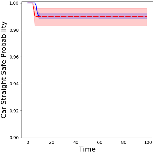
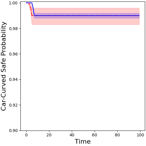
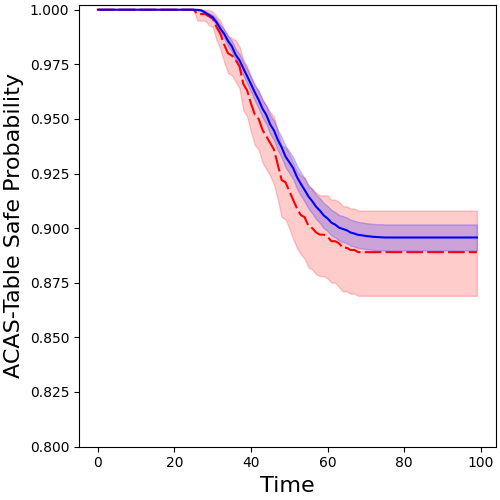
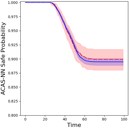
Figure 10. Evolution of safe state probability over time. Blue solid: GAS, red dashed: MCS.

6.1. Does GAS accurately estimate the probability that a vehicle will remain in a safe state over time?

Table 2 compares the distributions calculated by GAS and MCS for each benchmark state variable. Columns 3-4 compare the mean and standard deviation of the distributions at the final time step. Columns 5-6 show the maximum values of the KS statistic and Wasserstein metric over all time steps. For most state variables, the mean and standard deviation of the distributions match closely up to the final time step. This is also indicated by the low values of the Wasserstein metric and the conservative KS statistic. The largest difference is for the Car-Straight benchmark distance distribution. This occurs because the GAS model and the original vehicle model converge towards slightly different states around the center of the safe state space in later time steps. However, during the initial time steps where more simulated vehicles are in danger of entering unsafe states, the KS statistic does not exceed 0.15. A similar phenomenon affects the ACAS-NN downrange distance variable. For ACAS-Table, the GAS and original vehicle models occasionally turn in different directions to avoid an intruder approaching head-on, in situations where turning in either direction is equally beneficial. This leads to a large deviation in the heading variable.

Figure 10 shows how the probability that the vehicle remains in a safe state evolves over time. The blue solid and red dashed plots show the probability estimates obtained using GAS and MCS, respectively. The shaded region around each plot shows the 95% bootstrap confidence interval. Because we use $10\times$ more samples when estimating safe state probability with GAS as compared to MCS, the sampling error is smaller for GAS, which leads to a smaller confidence interval. Since GAS approximates the behavior of the vehicle model, as opposed to under/over approximation of reachable states, GAS’s safe state probability estimate can be on either side of the MCS estimate.

Table 4 shows the metrics we use to measure the similarity of the safe state probabilities from Figure 10. Column 2 shows the number of time steps for which the t-test “passed”, meaning that we could not reject the null hypothesis that the probabilities are equal. Column 3 shows the $\ell_{2}$ error, and Column 4 shows the cross-correlation. The similarity of the state distributions leads directly to the similarity of the safe state probability for most time steps.

We extended the Crop-Monitor and Car benchmark experiments to 500 time steps to confirm that the safe state probability does not deviate after 100 time steps. We did not similarly extend the ACAS experiments as the ACAS system is primarily relevant as the aircraft approach each other.

In conclusion, the vehicle state distributions that we estimate using GAS closely resemble those that we estimate using MCS, even after 100 time steps. Consequently, the vehicle safe state probability estimate is also similar between the two approaches.

Table 3. Metrics for comparing the probability of remaining in a safe state

Benchmark	t-test	$\ell_{2}$ err	X-Cor
Crop-Monitor	99/100	0.004	0.974
Car-Straight	97/100	0.001	0.862
Car-Curved	98/100	0.001	0.865
ACAS-Table	100/100	0.007	0.998
ACAS-NN	100/100	0.003	0.999

Table 4. Maximum difference in sensitivity indices

Benchmark	$\mathbf{x_{0}\!\rightarrow\!y_{1}}$	$\mathbf{x_{0}\!\rightarrow\!dy_{0}}$
Crop-Monitor	0.00003	0.0004
Car-Straight	0.0002	0.006
Car-Curved	0.00003	0.003
ACAS-Table	0.00001	0.009
ACAS-NN	0.00002	0.061

6.2. Does GAS accurately estimate global sensitivity indices of the vehicle model?

Table 4 presents the maximum difference between sensitivity indices calculated using $M_{\mathit{GPC}}$ and those calculated using $M^{\prime}_{V}$. Column 2 is for the sensitivity of state variables in time step 1 to those in time step 0 ($x_{0}\!\rightarrow\!y_{1}$) and Column 3 is for the sensitivity of the change in the state variables ($x_{0}\!\rightarrow\!dy_{0}$ where $dy_{0}\!=\!y_{1}\!-\!y_{0}$). The sensitivity indices calculated by $M_{\mathit{GPC}}$ and $M^{\prime}_{V}$ match closely.

Figure 11 shows an example visual comparison of sensitivity indices calculated by GAS and MCS for the sensitivity of the change in state between time step 0 and 1 to the initial state in time step 0 for Crop-Monitor. The input variables include the heading and distance at time step 0, and the two components of the raw sample that is transformed into the perception neural network output distribution sample. The output variables are the heading and distance at time step 1. There is one sensitivity index corresponding to each input/output variable pair. The blue solid line shows the sensitivity calculated analytically by GAS, the blue dotted line shows the sensitivity calculated empirically using the GAS model, and the red dashed line shows the sensitivity calculated empirically using $M^{\prime}_{V}$. In each subplot, the X-Axis shows the number of samples used for empirical estimation, while the Y-Axis shows the calculated sensitivity index. As the number of estimation samples is increased, the sensitivity indices calculated via estimation converge towards those calculated analytically. About $10^{6}$ samples are needed for convergence.

​

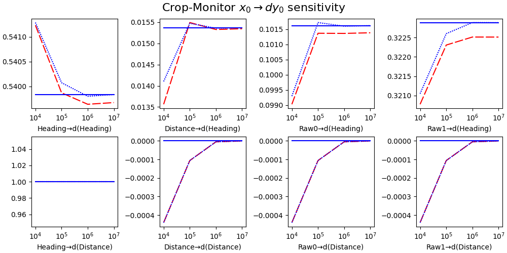
Figure 11. Calculated sensitivity index comparison. Blue solid: GAS (analytical method), blue dotted: GAS (empirical method), red dashed: MCS.

In conclusion, GAS enables precise global sensitivity analysis of vehicle models.

6.3. How do the parameters of the GAS perception model affect its accuracy?

Table 5 describes the effects of changing the perception model parameters $G$ and $N_{i}$. Column 1 presents the value of the parameter. Columns 2-4 present the maximum KS statistic and Wasserstein metric ($\times 100$) for the Crop-Monitor, Car-Straight, and Car-Curved benchmarks, respectively. Column 5 presents the estimated speedup caused by changing the parameter value, calculated based on the reduction in the number of images that must be captured and processed. We exclude the ACAS benchmarks as they do not use a perception model.

We focus on the cases where the error metrics change by 10% or more. While the grid size $G$ can be reduced to $9\times 9$ without much loss of accuracy, further reducing it to $7\times 7$ increases the error for all benchmarks. Similarly, reducing the number of images captured at each grid point ($N_{i}$) to 225 does not cause much loss of accuracy, but further reducing it to 100 images increases the error for all benchmarks. We prefer to err on the side of caution by collecting 350 images over a $11\times 11$ grid. The minimal change in accuracy caused by increasing $G$ from $9\times 9$ to $11\times 11$ or increasing $N_{i}$ from 225 to 350 also shows that further increases are unlikely to improve the accuracy of GAS.

In conclusion, perception model parameters can have a significant effect on the end-to-end results of GAS, and we must choose them carefully for optimal accuracy.

Table 5. Effect of changing perception model parameters on accuracy. An asterisk (*) indicates the primary value used in our evaluation. Changes of 10% or more are highlighted.

Parameter	$\mathbf{KS_{max}\!\times\!10^{2}/Wass_{max}\!\times\!10^{2}}$									Relative
Value	C-Mon			C-Str			C-Cur			Speedup
Ground truth grid dimensions ($G$)
$7\times 7$	20.3	/	2.43	46.8	/	9.63	23.8	/	3.24	$2.5\times$
$9\times 9$	12.2	/	2.25	42.4	/	8.39	16.2	/	2.00	$1.5\times$
$11\times 11$*	13.8	/	2.37	41.1	/	7.97	17.0	/	2.23	$1.0\times$
Images captured per grid point ($N_{i}$)
100	33.1	/	2.34	49.6	/	9.77	18.7	/	2.59	$3.5\times$
225	16.1	/	2.35	40.5	/	7.91	17.0	/	2.43	$1.6\times$
350*	13.8	/	2.37	41.1	/	7.97	17.0	/	2.23	$1.0\times$

6.4. Is GAS faster compared to Monte Carlo Simulation?

Table 6. Time usage for constructing $M_{\mathit{GPC}}$

Benchmark	$\mathbf{t_{dat}}$	$\mathbf{t_{per/anc}}$	$\mathbf{t_{GPC}}$
Crop-Monitor	8.5h	1.1s	1.4s
Car-Straight	3.3h	1.1s	1.4s
Car-Curved	3.1h	1.1s	1.4s
ACAS-Table	N/A	0.3s	0.3s
ACAS-NN	N/A	0.3s	0.4s

Table 7. Time usage for state distribution estimation

Benchmark	$\mathbf{t_{MCS}}$	$\mathbf{t_{GAS{}}}$
Crop-Monitor	19.5h	8.5h	($2.3\times$)
Car-Straight	6.8h	3.3h	($2.1\times$)
Car-Curved	6.5h	3.1h	($2.1\times$)
ACAS-Table	8.0s	1.1s	($7.3\times$)
ACAS-NN	10.7s	1.2s	($8.9\times$)

Table 8. Time usage for sensitivity analysis (excluding $t_{\mathit{dat}}$ and $t_{\mathit{per}}$ from Table 7)

Benchmark	$\mathbf{t^{emp}_{MCS}}$	$\mathbf{t^{emp}_{GAS{}}}$		$\mathbf{t^{ana}_{GAS{}}}$
Crop-Monitor	9.5s	6.2s	($1.3\times$)	11.4s	($0.7\times$)
Car-Straight	9.7s	6.2s	($1.3\times$)	11.4s	($0.8\times$)
Car-Curved	9.8s	6.2s	($1.3\times$)	11.3s	($0.8\times$)
ACAS-Table	5.2s	5.6s	($0.9\times$)	3.3s	($1.6\times$)
ACAS-NN	4.8s	5.3s	($0.9\times$)	3.1s	($1.5\times$)

GAS model construction.

Table 7 shows the time required to construct the GAS model. Column 1 shows the benchmark, Column 2 shows the time required to gather training data for the perception model as necessary, Column 3 shows the time required to create the perception and/or ancillary model as necessary, and Column 4 shows the time required to create $M_{\mathit{GPC}}$. While creating the perception, ancillary, and GPC models takes a few seconds, gathering the training data for the perception model takes several hours. As shown in Section 6.3, reducing perception model parameters such as $|G|$ and $N_{i}$ can reduce this time, but can also lead to a reduction in accuracy.

State distribution estimation.

Table 7 shows the time required by GAS and MCS for state distribution estimation. Column 1 shows the benchmark. Column 2 shows the time required for using $M_{V}$ for state distribution estimation. Column 3 shows the total time required by GAS – this includes the total time required to construct $M_{\mathit{GPC}}$ (from Table 7) and then evaluate it for state distribution estimation via Algorithm 4. Column 3 also shows the speedup of GAS over MCS. The costly process of gathering and processing images contributes to over 99% of $t_{\mathit{MCS}}$ for the Crop-Monitor and Car benchmarks. While increasing $N_{s}$ or $T$ increases $t_{\mathit{MCS}}$ significantly, the corresponding increase in $t_{\mathit{GAS{}}}$ is negligible as the time required to create the perception model is independent of $N_{s}$ and $T$. Consequently, the speedup of GAS for state distribution estimation increases for longer experiments or higher number of samples. For the ACAS benchmarks, the control component of $M_{V}$ contributes to over 90% of $t_{\mathit{MCS}}$. $M_{\mathit{GPC}}$ is faster than even the dynamics component of $M_{V}$, leading to significant speedups for these benchmarks.

Sensitivity analysis.

Table 8 shows the time required by GAS and MCS for sensitivity analysis. Column 1 shows the benchmark. Columns 2-3 show the required for calculating all sensitivity indices empirically with $M^{\prime}_{V}$ and $M_{\mathit{GPC}}$ respectively. Column 4 shows the time required calculating all sensitivity indices analytically with $M_{\mathit{GPC}}$. Columns 3-4 also show the speedup of GAS for the two approaches using $M_{\mathit{GPC}}$. Since both $M^{\prime}_{V}$ and $M_{\mathit{GPC}}$ use the perception model for the first three benchmarks, we exclude the time required to train and construct the perception model for those benchmarks. The replacement of the perception system by the perception model significantly speeds up $M^{\prime}_{V}$ as compared to $M_{V}$ and also enables vectorization. As this optimized version is the baseline for sensitivity indices calculation, the speedup of GAS for this application is lower than that for distribution estimation. While the analytical and empirical methods for calculating sensitivity using $M_{\mathit{GPC}}$ have similar accuracy, different methods are faster for different benchmarks.

Rapid iteration.

For the first three benchmarks, if the perception system is altered, GAS must create a new perception and GPC model. Consequently, while the speedup of GAS stays the same, the total amount of time saved over MCS increases with each iterative change. If only the vehicle control or dynamics are altered, then GAS does not need to create a new perception model. Because gathering data for the perception model is the major contributor to the runtime of GAS as shown in Tables 7 and 7, this allows vehicle developers to rapidly make changes to the control and dynamics systems of the vehicle and reanalyze the system with these changes within seconds.

In conclusion, GAS provides geometric mean speedups of $3.7\times$ for state distribution estimation and $1.4\times$ for sensitivity analysis. Increasing the number of samples or time steps or using GAS for rapid iteration during development further increases this speedup.

7. Discussion

7.1. Scalability

The GPC polynomial model must consider all possible interactions between state variables, and can suffer from the “curse of dimensionality” (combinatorial explosion of the number of polynomial terms). This is a general limitation of GPC, for which researchers in engineering applications have proposed solutions such as low-rank approximation (Konakli and Sudret, 2015).

Another solution is to omit higher-order polynomial terms in which multiple state variables interact (Feinberg and Langtangen, [n. d.]). Figure 12 shows the effects of this polynomial truncation approach for an order 4 GPC model. For both plots, the X-Axis shows the number of dimensions in the state space. The Y-Axis of the left plot shows the number of polynomial terms in the constructed GPC model, and the Y-Axis of the right plot shows the model construction time. The dashed red lines and the solid blue lines show the results for the full polynomial and the truncated polynomial, respectively. The speedup from truncation increases rapidly with dimensionality. Critically, this method retains lower-order interaction terms, ensuring that the constructed GPC model can still account for interactions between state variables (albeit to a lesser degree of fidelity).

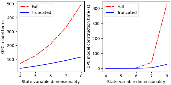
Figure 12. Effect of truncation on GPC model terms and construction time for an order 4 GPC model.

7.2. Limitations

GAS samples the provided environment distribution $\mathcal{D}_{E}$ when generating training data for the perception model in Algorithm 1. If GAS uses the perception model created for $\mathcal{D}_{E}$ to create a GPC model for a scenario with a significantly different environment distribution $\mathcal{D}_{E}^{\prime}$, it can lead to a reduction in accuracy of the final GPC model. To prevent this issue, we must carefully choose $\mathcal{D}_{E}$ to represent the distribution of environments the vehicle is expected to operate in. Even if creating a new perception model is necessary, we may be able to partially reuse existing training data from $\mathcal{D}_{E}$ that also fits into $\mathcal{D}_{E}^{\prime}$, reducing the additional time required to create the new perception model.

To construct the GPC model in Algorithm 3, all component distributions of the multivariate distribution $J$ must have corresponding orthogonal polynomials. This is true for a wide variety of distributions such as the uniform, normal, beta, and gamma distributions. We must ensure that all input variables for the GPC model are independent and are instances of these distributions. The wide variety of supported distributions is usually sufficient for modeling relevant input variables.

As GPC produces a polynomial model, its accuracy is limited when modeling functions with discontinuities or limited differentiability (Xiu, 2010, Theorem 3.6). Practically, this means that the GPC model will have a systemic bias that can be reduced, but not eliminated. Our evaluation shows that GAS’s hyperparameters must be carefully chosen to maximize accuracy while still providing speedups over MCS. However, once the ideal hyperparameters are found for modeling a particular vehicle system, it is possible to reuse them when making iterative changes to the vehicle model.

We demonstrate the applicability of GAS to autonomous vehicle scenarios with various structures and associated challenges. However, the applicability and efficiency of GAS for arbitrary autonomous vehicle scenarios is an open question and an interesting topic for future investigation.

7.3. Alternative formulations

The GPC model construction process in Algorithm 3 evaluates the abstracted vehicle model at specific quadrature nodes. Instead of constructing a perception model as in Section 4.2, we attempted to directly calculate and use the actual perception neural network output distributions at these quadrature nodes. However, if the quadrature nodes change (e.g., by changing the state distribution or order of GPC), then new images must be captured and processed for the new quadrature nodes. In contrast, the perception model can be directly reused as it is agnostic to the quadrature nodes.

We also experimented with replacing only parts of $M^{\prime}_{V}$ with GPC as follows: first, we replaced the perception system with the perception model to create $M^{\prime}_{V}$ as in Section 4.2. Then, instead of replacing all of $M^{\prime}_{V}$ with a GPC model as in Section 4.3, we replaced only the vehicle control and dynamics systems (as the perception system had already been replaced by a polynomial model $M_{\mathit{per}}$). While the accuracy of this approach was the same as our main approach, the partially replaced model was about $3\times$ slower than the fully replaced model during evaluation for all benchmarks.

8. Related Work

Analysis and verification of vehicle systems.

DryVR (Fan et al., 2017) is a system for verifying the safety of vehicle models that consist of a whitebox mode-switching control system composed with a blackbox dynamics system. DryVR obtains multiple samples from the blackbox dynamics and uses it give an over-approximate guarantee on the reachable set of states. In comparison, GAS focuses on perception and control systems which include blackbox components such as neural networks.

Jha et al. (Jha et al., 2018) and DeepDECS (Calinescu et al., 2022) analyze perception system uncertainty to create a correct by synthesis controller that satisfies a temporal logic safety constraint. GAS allows us to estimate the safety of existing, well known controllers for broad applications. Althoff et al. (Althoff and Dolan, 2014) focus on online verification of vehicle safety properties to adapt to unique traffic situations, assuming an upper bound on the noise of the perception system. In contrast, GAS allows the programmer to directly specify the perception system, and handles the dynamic nature of perception error through the perception model.

Musau et al. (Musau et al., 2022) complement complex neural network controllers with a safety controller which takes over if a runtime reachability analysis detects a potential collision. GAS’s state distribution estimates can be used to determine the degree of reliability of the neural network controller and therefore the optimal criteria for switching to the safety controller.

Yang et al. (Yang et al., 2022) propose a runtime system for detecting environmental conditions that were not part of the training data for a pre-trained perception system. Cheng et al. (Cheng et al., 2018) ensure that the training data covers different combinations of environmental factors, based on their relative importance. Scenic (Fremont et al., 2019) is a probabilistic language for specifying scenes in a virtual world for generating training images for perception neural networks in various environments. These works can be used when sampling images and/or prioritizing environments for training GAS’s perception model in order to ensure that GAS’s results are valid for the entire range of expected environments. For our evaluation, we used simple but realistic distributions of environmental parameters when generating images for training the perception model.

System simulation and modeling.

Kewlani et al. (Kewlani et al., 2012) create and use GPC surrogate models of vehicle dynamics components. Lin et al. (Lin et al., 2020) do the same using small neural networks as surrogate models. Replacing only vehicle dynamics with GPC surrogates leads to negligible speedup as the perception and control components of the vehicle model contributed to 90% or more of the runtime of the MCS analysis of our benchmarks. GAS creates GPC surrogate models of complete vehicle systems – the GPC model also replaces the expensive perception and control components. ARIsTEO (Menghi et al., 2020) uses abstraction refinement to create surrogate models of cyber-physical systems with low dimensional inputs. GAS handles high-dimensional image inputs by first creating a perception model, and then creates a surrogate model of the reduced-dimensionality abstract vehicle model.

Li et al. (Li et al., 2022) create small neural network surrogate models to calculate a fitness function for an autonomous driving system in various traffic scenarios. GAS’s surrogate models instead estimate the state distribution of the vehicle over time – information which can be used to calculate various fitness metrics. Michelmore et al. (Michelmore et al., 2020) evaluate the safety of end-to-end Bayesian Neural Network (BNN) controllers. While GAS’s perception model focuses on replacing regression DNNs, vehicle models with BNNs are an interesting target for extending GAS.

Simplification of complex perception and control systems.

Cheng et al. (Cheng et al., 2019) explore the correspondence between neural networks and polynomial regressions. Unlike their approach, GAS’s perception model only needs to predict the distribution of neural network outputs, instead of individual input-output relationships.

Several approaches focus on sound and complete verification of safety properties of ACAS-Xu neural networks (e.g., that the network will not give a COC advisory when an intruder aircraft is directly ahead on a collision course (Tran et al., 2020; Bak et al., 2020)). Others focus on providing probabilistic guarantees (e.g., bounding the probability that similar inputs will result in different advisories (Converse et al., 2020), or the probability of violating the safety property described above (Tran et al., 2023)). Unlike GAS and the approaches described below, these approaches focus on checking safety properties of the networks in isolation, that is, they do not take into account how the aircraft moves over time.

Several other recent approaches (e.g., (Julian and Kochenderfer, 2019; Bak and Tran, 2022; Manzanas Lopez et al., 2023)) focus on deterministically verifying properties of a closed-loop system containing ACAS-Xu neural networks and aircraft dynamics. In particular, Bak and Tran (Bak and Tran, 2022) checked the safety of the neural networks from (Julian et al., 2019) in 32 minutes on a 128 core machine. In contrast to those approaches, GAS does simulation-based probabilistic testing of ACAS-Xu neural networks coupled with aircraft dynamics. While GAS can find unsafe scenarios, it cannot provide non-probabilistic safety guarantees. Julian et al. (Julian et al., 2019) performed 1.5 million simulations to test their ACAS-Xu neural network, and Owen and Kochenderfer (Owen and Kochenderfer, 2016) performed 10 million simulations to determine whether horizontal or vertical advisories are safer in different states. We view GAS as a useful tool for speeding up such simulations and sanity checks of the closed-loop aircraft system when making experimental changes to it, before moving on to full verification.

Ghosh et al. (Ghosh et al., 2019) iteratively synthesize perception models and controllers guided by counterexamples to temporal logic safety properties. Hsieh et al. (Hsieh et al., 2022) create a perception model where the mean is calculated using piecewise linear regression and the allowable variance is calculated based on the controller code using program analysis tools like CBMC. Unlike these works, GAS’s perception model is independent of the controller, and can be reused without requiring additional sampling when iterative changes are made to the controller during development.

9. Conclusion

We present GAS, the first approach for using Generalized Polynomial Chaos (GPC) to analyze a complete autonomous vehicle system which composes complex perception and/or control components with vehicle dynamics. GAS first creates a model of the perception subsystem and uses it to generate a surrogate model of the entire vehicle system. GAS accurately models the system while being $3.7\times$ faster on average for state distribution estimation and $1.4\times$ faster on average for sensitivity analysis than Monte Carlo Simulation on five scenarios used in agricultural vehicles, self driving cars, and unmanned aircraft. We anticipate that GAS can augment or partially replace simulation-based workflow in tasks that require iterative modifications or continuous re-execution of the model – for example, during vehicle development.

References

- (1)
- Althoff and Dolan (2014) Matthias Althoff and John M. Dolan. 2014. Online Verification of Automated Road Vehicles Using Reachability Analysis. IEEE Transactions on Robotics 30 (2014), 903–918.
- Bak and Tran (2022) Stanley Bak and Hoang-Dung Tran. 2022. Neural Network Compression of ACAS Xu Early Prototype Is Unsafe: Closed-Loop Verification Through Quantized State Backreachability. In NASA Formal Methods.
- Bak et al. (2020) Stanley Bak, Hoang-Dung Tran, Kerianne Hobbs, and Taylor T. Johnson. 2020. Improved Geometric Path Enumeration for Verifying ReLU Neural Networks. In Computer Aided Verification.
- Calinescu et al. (2022) Radu Calinescu, Calum Imrie, Ravi Mangal, Corina Păsăreanu, Misael Alpizar Santana, and Gricel Vázquez. 2022. Discrete-Event Controller Synthesis for Autonomous Systems with Deep-Learning Perception Components. arXiv:2202.03360 [cs.LG]
- Cheng et al. (2018) Chih-Hong Cheng, Chung-Hao Huang, and Hirotoshi Yasuoka. 2018. Quantitative Projection Coverage for Testing ML-enabled Autonomous Systems. In Automated Technology for Verification and Analysis (ATVA).
- Cheng et al. (2019) Xi Cheng, Bohdan Khomtchouk, Norman Matloff, and Pete Mohanty. 2019. Polynomial Regression As an Alternative to Neural Nets. arXiv:1806.06850 [cs.LG]
- Converse et al. (2020) Hayes Converse, Antonio Filieri, Divya Gopinath, and Corina S. Pasareanu. 2020. Probabilistic Symbolic Analysis of Neural Networks. In ISSRE.
- Dosovitskiy et al. (2017) Alexey Dosovitskiy, German Ros, Felipe Codevilla, Antonio Lopez, and Vladlen Koltun. 2017. CARLA: An Open Urban Driving Simulator. In Proceedings of the 1st Annual Conference on Robot Learning. 1–16.
- Du et al. (2020) Peter Du, Zhe Huang, Tianqi Liu, Tianchen Ji, Ke Xu, Qichao Gao, Hussein Sibai, Katherine Driggs-Campbell, and Sayan Mitra. 2020. Online Monitoring for Safe Pedestrian-Vehicle Interactions. In IEEE 23rd International Conference on Intelligent Transportation Systems (ITSC).
- Ernst et al. (2012) Oliver Ernst, Antje Mugler, Hans-Jörg Starkloff, and Elisabeth Ullmann. 2012. On the convergence of generalized polynomial chaos expansions. ESAIM: Mathematical Modelling and Numerical Analysis 46 (2012).
- Fan et al. (2017) Chuchu Fan, Bolun Qi, Sayan Mitra, and Mahesh Viswanathan. 2017. DryVR: Data-Driven Verification and Compositional Reasoning for Automotive Systems. In Computer Aided Verification, 29th International Conference.
- Feinberg and Langtangen ([n. d.]) Jonathan Feinberg and Hans Petter Langtangen. [n. d.]. Truncation scheme - chaospy. https://chaospy.readthedocs.io/en/master/user_guide/polynomial/truncation_scheme.html.
- Feinberg and Langtangen (2015) Jonathan Feinberg and Hans Petter Langtangen. 2015. Chaospy: An open source tool for designing methods of uncertainty quantification. Journal of Computational Science 11 (2015).
- Fremont et al. (2019) Daniel J. Fremont, Tommaso Dreossi, Shromona Ghosh, Xiangyu Yue, Alberto L. Sangiovanni-Vincentelli, and Sanjit A. Seshia. 2019. Scenic: A Language for Scenario Specification and Scene Generation. In Proceedings of the 40th ACM SIGPLAN Conference on Programming Language Design and Implementation.
- Ghosh et al. (2019) Shromona Ghosh, Yash Vardhan Pant, Hadi Ravanbakhsh, and Sanjit A. Seshia. 2019. Counterexample-Guided Synthesis of Perception Models and Control. https://arxiv.org/abs/1911.01523
- Hsieh et al. (2022) Chiao Hsieh, Yangge Li, Dawei Sun, Keyur Joshi, Sasa Misailovic, and Sayan Mitra. 2022. Verifying Controllers with Vision-based Perception Using Safe Approximate Abstractions. In EMSOFT.
- Jha et al. (2018) Susmit Jha, Vasumathi Raman, Dorsa Sadigh, and Sanjit Seshia. 2018. Safe Autonomy Under Perception Uncertainty Using Chance-Constrained Temporal Logic. Journal of Automated Reasoning 60 (2018), 43–62.
- Julian and Kochenderfer (2019) Kyle D Julian and Mykel J Kochenderfer. 2019. Guaranteeing safety for neural network-based aircraft collision avoidance systems. In The 17th IEEE International Conference on Dependable, Autonomic and Secure Computing (DASC).
- Julian et al. (2019) Kyle D. Julian, Mykel J. Kochenderfer, and Michael P. Owen. 2019. Deep Neural Network Compression for Aircraft Collision Avoidance Systems. Journal of Guidance, Control, and Dynamics 42 (2019).
- Kewlani et al. (2012) Gaurav Kewlani, Justin Crawford, and Karl Iagnemma. 2012. A polynomial chaos approach to the analysis of vehicle dynamics under uncertainty. Vehicle System Dynamics 50 (2012).
- Koenig and Howard (2004) Nathan Koenig and Andrew Howard. 2004. Design and Use Paradigms for Gazebo, An Open-Source Multi-Robot Simulator. In IEEE International Workshop on Intelligent Robots and Systems (IROS).
- Konakli and Sudret (2015) Katerina Konakli and Bruno Sudret. 2015. Uncertainty Quantification in High Dimensional Spaces with Low-Rank Tensor Approximations. In 1st International Conference on Uncertainty Quantification in Computational Sciences and Engineering.
- Li et al. (2022) Renjue Li, Tianhang Qin, Pengfei Yang, Cheng-Chao Huang, Youcheng Sun, and Lijun Zhang. 2022. Safety Analysis of Autonomous Driving Systems Based on Model Learning. https://arxiv.org/abs/2211.12733
- Lin et al. (2020) Jingliang Lin, Haiyan Li, Yunbao Huang, Zeying Huang, and Zhiqian Luo. 2020. Adaptive Artificial Neural Network Surrogate Model of Nonlinear Hydraulic Adjustable Damper for Automotive Semi-Active Suspension System. IEEE Access 8 (2020).
- Manzanas Lopez et al. (2023) Diego Manzanas Lopez, Taylor T. Johnson, Stanley Bak, Hoang-Dung Tran, and Kerianne L. Hobbs. 2023. Evaluation of Neural Network Verification Methods for Air-to-Air Collision Avoidance. Journal of Air Transportation 31 (2023).
- MaybeShewill-CV ([n. d.]) MaybeShewill-CV. [n. d.]. MaybeShewill-CV/lanenet-lane-detection: Unofficial implemention of the lanenet model for real time lane detection. https://github.com/MaybeShewill-CV/lanenet-lane-detection.
- Menghi et al. (2020) Claudio Menghi, Shiva Nejati, Lionel Briand, and Yago Isasi Parache. 2020. Approximation-refinement testing of compute-intensive cyber-physical models: An approach based on system identification. In Proceedings of the ACM/IEEE 42nd International Conference on Software Engineering.
- Michelmore et al. (2020) Rhiannon Michelmore, Matthew Wicker, Luca Laurenti, Luca Cardelli, Yarin Gal, and Marta Kwiatkowska. 2020. Uncertainty Quantification with Statistical Guarantees in End-to-End Autonomous Driving Control. In IEEE International Conference on Robotics and Automation (ICRA).
- Musau et al. (2022) Patrick Musau, Nathaniel Hamilton, Diego Manzanas Lopez, Preston Robinette, and Taylor T. Johnson. 2022. On Using Real-Time Reachability for the Safety Assurance of Machine Learning Controllers. In IEEE International Conference on Assured Autonomy (ICAA).
- Owen and Kochenderfer (2016) Michael P. Owen and Mykel J. Kochenderfer. 2016. Dynamic logic selection for unmanned aircraft separation. In 2016 IEEE/AIAA 35th Digital Avionics Systems Conference (DASC).
- Pan and Rajan (2020) Rangeet Pan and Hridesh Rajan. 2020. On Decomposing a Deep Neural Network into Modules. In ESEC/FSE.
- Robert and Casella (2004) Christian P Robert and George Casella. 2004. Monte Carlo statistical methods. Vol. 2. Springer.
- Sivakumar et al. (2021) Arun Narenthiran Sivakumar, Sahil Modi, Mateus Valverde Gasparino, Che Ellis, Andres Eduardo Baquero Velasquez, Girish Chowdhary, and Saurabh Gupta. 2021. Learned Visual Navigation for Under-Canopy Agricultural Robots. arXiv:2107.02792 [cs.RO]
- Sobol (2001) I.M Sobol. 2001. Global sensitivity indices for nonlinear mathematical models and their Monte Carlo estimates. Mathematics and Computers in Simulation 55 (2001).
- Tran et al. (2023) Hoang-Dung Tran, Sungwoo Choi, Hideki Okamoto, Bardh Hoxha, Georgios Fainekos, and Danil Prokhorov. 2023. Quantitative Verification for Neural Networks Using ProbStars. In Proceedings of the 26th ACM International Conference on Hybrid Systems: Computation and Control.
- Tran et al. (2020) Hoang-Dung Tran, Xiaodong Yang, Diego Manzanas Lopez, Patrick Musau, Luan Viet Nguyen, Weiming Xiang, Stanley Bak, and Taylor T. Johnson. 2020. NNV: The Neural Network Verification Tool for Deep Neural Networks and Learning-Enabled Cyber-Physical Systems. In Computer Aided Verification, 32nd International Conference.
- Xiu (2010) Dongbin Xiu. 2010. Numerical Methods for Stochastic Computations: A Spectral Method Approach. Princeton University Press.
- Yang et al. (2022) Yahan Yang, Ramneet Kaur, Souradeep Dutta, and Insup Lee. 2022. Interpretable Detection of Distribution Shifts in Learning Enabled Cyber-Physical Systems. In ACM/IEEE 13th International Conference on Cyber-Physical Systems.