A Nonparametric Framework for Online Stochastic Matching with Correlated Arrivals Ali Aouad London Business School, Regent’s Park, London, United Kingdom, aaouad@london.edu Will Ma Graduate School of Business, Columbia University, New York, NY 10027, wm2428@gsb.columbia.edu

The design of online policies for stochastic matching and revenue management settings is usually bound by the Bayesian prior that the demand process is formed by a fixed-length sequence of queries with unknown types, each drawn independently. This assumption of serial independence implies that the demand of each type, i.e., the number of queries of a given type, has low variance and is approximately Poisson-distributed. Thus, matching policies are often based on “fluid” LPs that only use the expectations of these distributions.

This paper explores alternative stochastic models for online matching that allow for nonparametric, higher variance demand distributions. We propose two new models, Indep and Correl, that relax the serial independence assumption in different ways by combining a nonparametric distribution for the demand with standard assumptions on the arrival patterns—adversarial or random-order. In our Indep model, the demand for each type follows an arbitrary distribution, while being mutually independent across different types. In our Correl model, the total demand follows an arbitrary distribution, and conditional on the sequence length, the type of each query is drawn independently. In both settings, we show that the fluid LP relaxation based on only expected demands can be an arbitrarily bad benchmark for algorithm design. We develop tighter LP relaxations for the Indep and Correl models that leverage the exact distribution of the demand, leading to matching algorithms that achieve constant-factor performance guarantees under adversarial and random-order arrivals. More broadly, our paper provides a data-driven framework for expressing demand uncertainty (i.e., variance and correlations) in online stochastic matching models.

Online matching, demand uncertainty, competitive ratio, LP rounding.

1 Introduction

In the online matching problem, queries of one of $m$ types arrive over a finite time horizon and must be irrevocably served by up to one of $n$ capacity-constrained resources. A known reward of $r_{i,j}$ (possibly $r_{i,j}=0$) is collected each time a query of any type $j=1,\ldots,m$ is served by any resource $i=1,\ldots,n$. The objective is to maximize the total reward collected over the time horizon.

The expansive area of online stochastic matching has focused on algorithm design under a model of serial independence, where there is a fixed-length sequence of queries $t=1,\ldots,T$ and their types are drawn independently over time. A major shortcoming of such a model, however, is that it imposes the total number of queries of any type $j$, which we call the demand $D_{j}$ for type $j$, to have a variance that is at most its mean, i.e.

$$\mathrm{Var}(D_{j}) \leq\mathbb{E}[D_{j}] \forall j\ .$$ (1)

In turn, inequality (1) implies that “fluid” policies, which make decisions using an LP that replaces each $D_{j}$ with its expectation, will perform well when all expected demands $\mathbb{E}[D_{j}]$ are large.

However, these are artifacts of the serial independence assumption, and inequality (1) does not naturally hold for many stochastic models used to inform operational decisions. When modeling unknown demand in supply chains, textbook examples use a Normal distribution with an arbitrary mean and standard deviation (Simchi-Levi et al. 2005). When managing revenue from different customer classes $j$, standard models allow the demands $D_{j}$ to be drawn from arbitrary distributions (Talluri and Van Ryzin 2004, Chap. 2.2), which are independent across $j$ but do not need to satisfy (1). In fact, Talluri and Van Ryzin (2004, Chap. 2.5) identify the same challenge when modeling how these customers arrive over time:

“Dynamic models [i.e. online stochastic matching] allow for an arbitrary order of arrival, with the possibility of interspersed arrivals of several classes […] the dynamic models require the assumption of Markovian (such as Poisson) [i.e. serial independence] arrivals to make them tractable. This puts restrictions on modeling different levels of variability in demand.”

As a concrete example, we observe first hand that property (1) may not hold on real-world data.

Example 1.1 (JD.com)

We conduct a simple analysis using a public data set released by the e-commerce platform JD.com (Shen et al. 2020). Taking the perspective of order fulfilment, we estimate the empirical mean and variance of weekly demand for the 40 highest-selling SKUs in the 40 largest locations. The empirical variance is larger the empirical mean for 86% of such SKUs and locations. Details of our analysis and further discussion are provided in Appendix 5.

In this paper, we overcome these modeling challenges by proposing a new approach which abolishes serial independence and assumption (1), allows for interleaved arrivals of different query types, and leads to tractable guarantees. Our general framework is simple and consists of two aspects:

1. A random variable ${\bf D}=(D_{1},\ldots,D_{m})$ is first drawn from a known distribution, which we call the demand vector and represents the number of queries $D_{j}$ of each type $j\in[m]$;

2. A separate process then specifies for any realization of ${\bf D}$ the arrival order.

We now present specific distributions and processes for (i) and (ii) above that will be considered in this paper. As discussed subsequently, not only does our approach generalize certain models studied in previous literature, but we also believe that separating out aspects (i) and (ii) can be useful for developing data-driven approaches to online matching.

Specific distributions for (i).

Allowing ${\bf D}$ to take an arbitrary distribution returns us to settings of online (non-stochastic) matching where nothing is known about ${\bf D}$, as we explain in Subsection 1.2. Thus, in this paper we consider two specific classes for the distribution of ${\bf D}$:

1. The demand $D_{j}$ of each type $j\in[m]$ is drawn independently from an arbitrary type-specific distribution (this is exactly the model noted in Talluri and Van Ryzin (2004, Chap. 2));

2. The total demand $D$ is first drawn from an arbitrary distribution, and then each query $t\in[D]$ independently draws a type from $\{1,\ldots,m\}$ according to a known probability vector ${\bf p}=(p_{1},\ldots,p_{m})$ satisfying $\sum_{j=1}^{m}p_{j}=1$ (note that $D=D_{1}+\cdots+D_{m}$).

Both Indep and Correl allow demands $D_{j}$ to have arbitrary marginal distributions whose variances are larger than their expectations. However, Indep and Correl capture different forms of correlations. In Indep, since the distribution of each demand entry $D_{j}$ can be arbitrary, observing a large number of arrivals of a given type $j$ so far may indicate more demand of that type in the future. Yet, there is no mutual information between the demands for different types, since the entries $D_{j}$ are independent across $j\in[m]$. That is, each type $j$ incurs an idiosyncratic shock in its demand $D_{j}$. By contrast, the Correl model allows for positive correlations across $j$, in that a high realization of $D$ leads to every demand $D_{j}$ being larger. This is motivated by an external shock, e.g., weather, that can simultaneously affect the demands of all types. These models are theoretically natural to study as they both generalize the well-studied model of online stochastic matching under Poisson arrivals, as we explain later.

Specific processes for (ii).

For any realization of ${\bf D}$, we now specify how the $D_{j}$ arrivals of each type $j$ can be interleaved in relation to other types. Here, let us consider two processes:

1. Adversarial: the $D=D_{1}+\cdots+D_{m}$ total queries arrive in an order chosen by an adversary;

2. Random-order: the $D=D_{1}+\cdots+D_{m}$ total queries arrive in a uniformly random order.

Processes 1-2 are presented in decreasing order of difficulty for algorithm design, with these arrival processes being widely used in the computer science literature. Process 1 is useful to develop algorithms with robust performance, regardless of the arrival order. This setting is relevant when the arrival order is hard to predict, as might be the case for bursty arrivals. By contrast, Process 2 imposes that query types are uniformly ordered, which allows the decision-maker to (ignoring computational constraints) maintain distributional knowledge of the arrival sequence. Therefore, the notion of an optimal policy is well-defined in this context.

Outline of results.

For edge-weighted online bipartite matching with adversarial arrivals, we show that under the Indep model of stochastic demand, there exists a 1/2-competitive polynomial-time online algorithm (Theorem 2.4). Our algorithm leverages a new “truncated” LP relaxation of the optimal offline matching, as we show that the typical fluid LP relaxation leads to a competitive ratio of 0 (Proposition 2.1). The algorithm also uses a new procedure for randomly routing the arrivals of a given type (whose demand is unknown a priori) to resources, which provides a loss-less rounding of a feasible solution to our truncated LP. Finally, we show that our competitive ratio of 1/2 cannot improve with asymptotic starting capacities for the resources (Proposition 2.5), due to the high-variance nature of Indep demand.

For edge-weighted online bipartite matching with random-order arrivals, under the Correl model where the total demand is unknown, any constant-factor competitive ratio is impossible. Accordingly, we focus on approximation ratios and derive a 1/2-approximate algorithm (Theorem 2.8), whose guarantee improves to 1 when starting capacities are large (Theorem 2.11). This algorithm leverages a new “conditional” LP that is a relaxation of the optimal online algorithm, relative to which the approximation ratio of 1/2 is tight (Proposition 2.10). Our algorithm necessarily adapts to the unfolding of the total demand $D$ in the Correl model—interestingly, we show that commonly-used policies which set non-adaptive acceptance thresholds for the resources lead to an approximation ratio of 0 (Proposition 2.9).

Organization of paper.

Statements of results for the Indep model are found in Subsection 2.1. Statements of results for the Correl model are found in Subsection 2.2. Our loss-less rounding scheme is detailed in Section 3. All proofs of specific statements, unless indicated otherwise, are deferred to the appendices. The analysis of JD.com data is presented in Section 5.

1.1 Further Discussions

Connection to Poisson arrival.

We call Poisson the online stochastic matching problem in continuous time where each type $j\in[m]$ arrives following an independent Poisson process of rate $\lambda_{j}$ over the time horizon $[0,1]$. It is not difficult to see that both the Indep and Correl models can capture Poisson as a special case. To reveal the connection with Poisson, suppose we operate under the random-order Process 2, but we further assume that each arrival has a timestamp in the horizon $[0,1]$. Under the Poisson model, we note that the demand $D_{j}$ of each type $j$ ends up having a distribution that is Poisson with expectation $\lambda_{j}$. Moreover, a basic property of stationary compound Poisson processes is that the density of arrivals is uniform over $[0,1]$ conditional on each realization of ${\bf D}$. This implies that any instance of Poisson with arrival rates $(\lambda_{j})_{j\in[m]}$ can be captured within our framework by Indep and random-order with arrival times, assuming that each demand entry $D_{j}$ follows a Poisson distribution with mean $\mathbb{E}[D_{j}]=\lambda_{j}$. Similarly, the split-and-combine property of Poisson processes straightforwardly implies that this Poisson instance has an equivalent representation within our Correl model, where $D$ is Poisson-distributed with mean $\mathbb{E}[D]=\lambda_{1}+\cdots+\lambda_{m}$ and $p_{j}=\lambda_{j}/\mathbb{E}[D]$ for all $j\in[m]$.

It is worth noting that the above reduction from Poisson to Indep and Correl has implications for other widely studied models of online stochastic matching. The recent advancement made by Huang and Shu (2021) in analyzing online stochastic matching problems with independent and identically distributed (IID) arrivals formalizes the idea that arrival processes formed by $T$ independently sampled query types can be approximated arbitrarily closely by the Poisson model. As the approximation error factor scales as $O(T^{-\frac{1}{2}})$ for a class of “natural” online algorithms, this reduction is efficient (i.e., polynomial-time and strict approximation-preserving) for algorithm design. This connection suggests that a deviation from the assumption of serial independence is inevitable to capture demand in a way that differs significantly from the Poisson model.

Data-driven applications.

We believe that our approach of separating out aspects (i) and (ii) could also be useful to devise data-driven policies for online matching. In matching settings, large variances in the total demand are caused by serial correlations over time, where many arrivals of a certain type within a short span beget more arrivals of that type in the near future. Although such patterns are captured by parametric families of self-exciting stochastic processes such as the Hawkes process (Laub et al. 2015), it might be difficult in practice to correctly specify and estimate a continuous-time stochastic process to quantify these effects. For example, it is likely that the underlying parameters of such processes will vary over time.

By contrast, we maintain a non-parametric approach with regards to the temporal aspects of the arrival patterns and focus on modeling the aggregate number of queries per type, a notion we refer to as the demand. In many practical scenarios, the distribution of the demand ${\bf D}$ is much easier to model and estimate since the decision-maker directly observes samples of ${\bf D}$ in the historical data. Moreover, our models Indep and Correl provide two simple ways to parameterize such distributions. Our framework still require us to specify a certain arrival pattern (ii), yet this element does not need to be explicitly estimated from data. Here, we consider two natural assumptions—adversarial and random-order—representing extreme cases: irregular arrival patterns that require robust online decisions and regularly paced arrivals that often yield better performance guarantees. The adversarial and random-order (without arrival times) models are also of theoretical interest in the online matching literature.

1.2 Related Work

Adversarial and random-order online matching.

Our work considers two specific classes of distributions, Indep and Correl, for the demand vector ${\bf D}$ which counts the number of arriving queries (or online vertices) of each type. Had we allowed ${\bf D}$ to take any distribution, then, for worst-case competitive ratios, this setting would be equivalent (by Yao’s minimax principle) to ${\bf D}$ being completely unknown. This would return us to the well-studied adversarial and random-order (with an unknown number of arrivals) models of online matching.

Under either of these models, when the rewards are edge-weighted as in our problem, no constant-factor competitive ratio is possible (Mehta 2013). To allow positive results under adversarial arrivals, researchers have added a free-disposal assumption (Feldman et al. 2009, Fahrbach et al. 2020) or derived parametric bounds (Ma and Simchi-Levi 2020). To allow positive results under random-order arrivals, researchers have assumed that the total number of arrivals is known, in which case a $1/e$-competitive algorithm exists (Kesselheim et al. 2013). We should note however that online matching was originally studied in the unweighted and vertex-weighted settings, which have a tight competitive ratio of $1-1/e$ for adversarial arrivals (Karp et al. 1990, Aggarwal et al. 2011). For random-order arrivals, tight results are not known, but the state-of-the-art guarantees are 0.696 for the unweighted setting (Mahdian and Yan 2011) and 0.662 for the vertex-weighted setting (Jin and Williamson 2021).

Online stochastic matching.

Our work proposes new models for specifying a prior distribution on the number of online vertices to arrive, contrasting with the standard model where each query in a fixed-length sequence is drawn independently from a distribution of types. In the edge-weighted setting, Alaei et al. (2012b) establish a competitive ratio of 1/2 when the type distributions are time-varying. Ehsani et al. (2018) derive an improved lower bound of $1-1/e$ when the arrival order is chosen uniformly at random (i.e., the random-order arrival pattern), rather than being fixed. The special case where types are drawn IID, in which case the arrival order does not matter, has also been extensively studied starting with the seminal works of Feldman et al. (2009) and Manshadi et al. (2012). Under an integral arrival rates assumption, the best-known guarantees are 0.705 for edge-weighted (Brubach et al. 2016) and 0.729 for vertex-weighted and unweighted (Brubach et al. 2016). Without this assumption, the best-known guarantees are 0.716 for vertex-weighted and unweighted (Huang et al. 2022).

Approximation ratios are also well-defined in online stochastic matching and can be different from competitive ratios, as we find for our Correl model. Recently, Papadimitriou et al. (2021) derive a 0.51-approximation for the setting of Alaei et al. (2012b), in which competitive ratios cannot breach 1/2.

Loss-less rounding schemes.

Our rounding scheme for the truncated LP adds to a short list of results that provide an exact, polynomially-solvable LP to represent a certain class of implementable (randomized) allocation policies—in our context, the truncated LP is exact for a fixed query type with random demand. Results in this spirit include the LP formulation by Alaei et al. (2012a) for the polytope of implementable interim allocation rules in multi-agent Bayesian auctions, which is essentially a polynomial-size lifted version of an earlier LP by Border (1991).

A well-known dependent rounding for the bipartite matching polytope is due to Gandhi et al. (2006). For the query-commit model of online bipartite matching, Gamlath et al. (2019a) propose an efficiently separable LP that tightly describes the distribution of implementable query-then-match policies for any fixed vertex. Online rounding methods have also been recently applied in adversarial online matching problems (Gamlath et al. 2019b, Buchbinder et al. 2021); these problems differ from ours in that we are rounding a fractional solution based on stochastic information of how many more vertices (of a homogeneous type) are going to arrive in the future.

Finally, Asadpour et al. (2020) recently derived an exact exponential-sized LP for the distribution of permutations over a given ground set based on Hall’s matching theorem (Hall 1987), and develop a relaxation that can be computed in polynomial time. This result also differs from ours because the fractional solution assigns (sets of) items to specific positions, whereas in our setting the LP solution merely indicates an aggregate probability for routing each item to some arriving query within the stochastic demand stream.

2 Theoretical Model and Results

Notation.

For a positive integer $n$, we let $[n]$ denote the set $\{1,\ldots,n\}$. We use $f\langle S\rangle$ to denote the image of a set $S$ through a function $f$. For random variables $(X,Y)$ defined in a joint probability space, we sometimes use $X(Y)$ to emphasize that the realization of $X$ depends on that of $Y$.

Model.

An instance $\mathcal{I}$ of our online stochastic matching model consists of the following parameters: the number of resource types $n$, the number of query types $m$, the corresponding reward values $(r_{i,j})_{i\in[n],j\in[m]}$, the starting capacities $(k_{i})_{i\in[n]}$, the distribution of the demand random variable ${\bf D}$, and a categorical variable for its arrival pattern which could be “adversarial ” or “random”. Each resource $i$ can be matched at most $k_{i}$ times. Meanwhile, ${\bf D}=(D_{j})_{j\in[m]}$ is a random vector denoting for each type $j\in[m]$ the total number of queries $D_{j}$ of that type to arrive. The total demand, defined as $D=D_{1}+\cdots+D_{m}$, is the length of the sequence of all queries.

We consider two classes of distributions, Indep and Correl, for the demand random variable ${\bf D}$. Under the first class, entries $D_{j}$ of ${\bf D}$ are drawn from arbitrary distributions, independently across $j$. We emphasize that each type $j\in[m]$ may have a different distribution for its demand $D_{j}$. Meanwhile, the second class allows for entries $D_{j}$ of ${\bf D}$ to be correlated in the following way: first the total demand $D$ is drawn from an arbitrary distribution, and then the types of these $D$ queries are specified by independent and identically distributed outcomes. Each type $j\in[m]$ is drawn with probability $p_{j}$, where we assume that $\sum_{j=1}^{m}p_{j}=1$. We use the notation $\mathcal{I}\in\textsc{Indep}$ or $\mathcal{I}\in\textsc{Correl}$ to indicate that the demand distribution for instance $\mathcal{I}$ falls under each of the above classes, respectively.

Finally, the arrival pattern will generate a sequence of query types $\sigma$ representing the arrival order of the $D=D_{1}+\cdots+D_{m}$ queries. In $\sigma$, each type $j$ has multiplicity $D_{j}$, i.e., appears exactly $D_{j}$ times. We denote by ${\cal S}({\bf D})$ the set of all such sequences, noting that $|{\cal S}({\bf D})|=\frac{D!}{D_{1}!\cdots D_{m}!}$.

Algorithms and performance.

An online algorithm provides a (randomized) policy for how to match queries on-the-fly, knowing only the instance $\mathcal{I}$ ahead of time. Specifically, the algorithm has access to the full distribution of the demand and the arrival pattern, but it does not know the specific realization of ${\bf D}$ and $\sigma$ until those are revealed by the sequence of queries. We let $\mathsf{ALG}_{\mathcal{I}}({\bf D},\sigma)$ denote the total rewards collected by the algorithm in expectation (over any randomness in the algorithm) when the demand vector realizes to ${\bf D}$ and the arrival order is $\sigma$.

Recall that $\sigma$ is determined by an arrival pattern associated with instance $\mathcal{I}$, which is either adversarial or random, in which case we write $\mathcal{I}\in\textsc{Adv}$ or $\mathcal{I}\in\textsc{Rand}$ respectively. Under adversarial order, an adversary chooses $\sigma$ to minimize $\mathsf{ALG}_{\mathcal{I}}({\bf D},\sigma)$ knowing both ${\bf D}$ and the algorithm being used (but not the realizations of its random bits). Therefore, if $\mathcal{I}\in\textsc{Adv}$ then we define the algorithm’s performance to be $\mathsf{ALG}(\mathcal{I}):=\mathbb{E}_{\bf D}[\inf_{\sigma\in{\cal S}({\bf D})}\mathsf{ALG}_{\cal I}({\bf D},\sigma)]$. Meanwhile, under random order, conditional on the realization of ${\bf D}$, the sequence $\sigma$ is equally likely to be any element in ${\cal S}({\bf D})$. Therefore, if $\mathcal{I}\in\textsc{Rand}$ then we define the algorithm’s performance to be $\mathsf{ALG}(\mathcal{I}):=\mathbb{E}_{{\bf D},\sigma}[\mathsf{ALG}_{\mathcal{I}}({\bf D},\sigma)]$. We note that algorithmic performance can always be made better for instances $\mathcal{I}\in\textsc{Rand}$ than for the corresponding instances in Adv.

Benchmarks.

We formalize standard benchmarks against which the performance of online algorithms is measured. We define $\mathsf{OFF}_{\mathcal{I}}({\bf D})$ as the maximum-weight offline matching that could have been made knowing the demand realization ${\bf D}$ in advance. Clearly, the offline matching does not depend on the arrival order $\sigma$. Consequently, the offline optimum, or prophet optimum, is the quantity $\mathsf{OFF}(\mathcal{I}):=\mathbb{E}_{{\bf D}}[\mathsf{OFF}_{\mathcal{I}}({\bf D})]$. For instances $\mathcal{I}\in\textsc{Rand}$, we also consider the online optimum $\mathsf{OPT}(\mathcal{I})$, corresponding to the performance of an optimal online algorithm without any restriction on computational time. This algorithm is defined as an exponentially-sized dynamic program that maximizes total expected rewards in each stage based on the prior on ${\bf D}$ and $\sigma$ and the information revealed thus far.

Competitive and approximation ratios.

For every $c\in[0,1]$, we say that an algorithm is $c$-competitive for a family of instances if $\mathsf{ALG}(\mathcal{I})/\mathsf{OFF}(\mathcal{I})\geq c$ for all such instances $\mathcal{I}$. The maximum constant $c$ for which this holds, i.e., the quantity $\inf_{\mathcal{I}}\mathsf{ALG}(\mathcal{I})/\mathsf{OFF}(\mathcal{I})$ with $\mathcal{I}$ restricted to that family, is sometimes referred to as the competitive ratio (for the family and algorithm in question). In this paper, we consider competitive ratios for families of instances constructed by specifying $\mathcal{I}\in\textsc{Indep}$ or $\mathcal{I}\in\textsc{Correl}$, and orthogonally by choosing $\mathcal{I}\in\textsc{Adv}$ or $\mathcal{I}\in\textsc{Rand}$, with otherwise no restrictions on $n$, $m$, the reward values $r_{i,j}$, or the distributions.

Similarly, when restricting attention to instances $\mathcal{I}\in\textsc{Rand}$, we also define a notion of approximation ratio, where the algorithm’s performance is normalized with respect to the online optimum $\mathsf{OPT}(\mathcal{I})$. For every $\alpha\in[0,1]$, we say that an algorithm is $\alpha$-approximate for a family of Rand instances if $\mathsf{ALG}(\mathcal{I})/\mathsf{OPT}(\mathcal{I})\geq\alpha$ for all such instances $\mathcal{I}$.

2.1 Results for Indep

In this subsection, we state our results for the Indep model. We first show that a standard approach for establishing competitive ratios, based on a fluid LP, fails. For any instance $\mathcal{I}$, let $\mathsf{LP}(\mathcal{I})$ denote the optimal objective value of the following LP:

$$\max\ \ \ \ \ \sum_{i=1}^{n}\sum_{j=1}^{m}r_{i,j}x_{i,j}$$ (2)

s.t. $$\sum_{j=1}^{m}x_{i,j}\leq k_{i} \forall i\in[n]$$ (3)

$$\sum_{i=1}^{n}x_{i,j}\leq\mathbb{E}[D_{j}] \forall j\in[m]$$ (4)

$$x_{i,j}\geq 0 \forall i\in[n],\forall j\in[m]\ .$$ (5)

The LP defined in (2)–(5) amounts to a simplified problem formulation where the stochastic demands of query types are replaced by deterministic quantities—their expectations. This relaxation has been the starting point for the design of constant-factor competitive algorithms in a rich literature on online stochastic matching problems. Similarly, this LP has served as a gold-standard upper bound for asymptotic performance analysis in the literature on revenue management. Indeed, it is well-known that $\mathsf{OPT}(\mathcal{I})\leq\mathsf{OFF}(\mathcal{I})\leq\mathsf{LP}(\mathcal{I})$ for all instances $\mathcal{I}$, and hence establishing that $\mathsf{ALG}(\mathcal{I})/\mathsf{LP}(\mathcal{I})\geq c$ for some constant $c>0$ over a class of instances $\mathcal{I}$ implies that $\mathsf{ALG}(\mathcal{I})/\mathsf{OFF}(\mathcal{I})\geq c$ and $\mathsf{ALG}(\mathcal{I})/\mathsf{OPT}(\mathcal{I})\geq c$ as well for all such $\mathcal{I}$.

We show that for instances $\mathcal{I}\in\textsc{Indep}$, the optimal objective of the fluid relaxation $\mathsf{LP}(\mathcal{I})$ can be arbitrarily larger than the offline performance $\mathsf{OFF}(\mathcal{I})$. Thus, in sharp contrast with existing models, this LP does not provide an appropriate yardstick for algorithm design.

Proposition 2.1

Under Indep, the fluid relaxation LP can be arbitrarily larger than the offline optimum, i.e., $\displaystyle\inf_{\mathcal{I}\in\textsc{Indep}}\frac{\mathsf{OFF}(\mathcal{I})}{\mathsf{LP}(\mathcal{I})}=0$. This holds even for the following restrictions of Indep: (i) $n=m=1$, or (ii) $n>1$, $m=1$, and ${\rm Pr}[D_{1}\leq\sum_{i=1}^{n}k_{i}]=1$.

Proposition 2.1 is proved in Subsection 6.1 by constructing a family of instances where the ratio between $\mathsf{OFF}({\cal I})$ and $\mathsf{LP}({\cal I})$ converges to zero. Construction (ii) further shows that a simple fix to the fluid LP does not suffice to obtain a benchmark comparable to the offline optimum. Now, under any arrival pattern and online algorithm, one must have $\mathsf{ALG}(\mathcal{I})\leq\mathsf{OFF}(\mathcal{I})$, and hence for any online algorithm the competitive ratio must satisfy $\inf_{\mathcal{I}\in\textsc{Indep}}\mathsf{ALG}(\mathcal{I})/\mathsf{LP}(\mathcal{I})\leq\inf_{\mathcal{I}\in\textsc{Indep}}\mathsf{OFF}(\mathcal{I})/\mathsf{LP}(\mathcal{I})=0$. In light of this, we introduce a tighter LP.

Definition 2.2

For any instance $\mathcal{I}$, we define $\mathsf{LP}^{\mathsf{trunc}}(\mathcal{I})$ as the optimal objective value of the following “truncated” LP:

$$\max\ \ \ \ \ \sum_{i=1}^{n}\sum_{j=1}^{m}r_{i,j}x_{i,j}$$ (6)

s.t. $$\sum_{j=1}^{m}x_{i,j}\leq k_{i} \forall i\in[n]$$ (7)

$$\sum_{i\in S}x_{i,j}\leq\mathbb{E}\left[\min\left\{D_{j},\sum_{i\in S}k_{i}\right\}\right] \forall S\subseteq[n],\forall j\in[m]$$ (8)

$$x_{i,j}\geq 0 \forall i\in[n],\forall j\in[m]\ .$$ (9)

It is straightforward to see that $\mathsf{LP}^{\mathsf{trunc}}(\mathcal{I})$ is a tightening of the fluid relaxation $\mathsf{LP}({\cal I})$, i.e., $\mathsf{LP}^{\mathsf{trunc}}(\mathcal{I})\leq\mathsf{LP}(\mathcal{I})$ for all $\mathcal{I}$, through a comparison of constraints (8) and (4), while noticing that all other ingredients of the formulation are unchanged. Indeed, by specifying $S=[n]$ in constraint (8), we obtain that any feasible solution of $\mathsf{LP}^{\mathsf{trunc}}(\mathcal{I})$ satisfies

$$\sum_{i=1}^{n}x_{i,j}\leq{\mathbb{E}}\left[\min\left\{D_{j},\sum_{i=1}^{n}k_{i}\right\}\right]\leq{\mathbb{E}}\left[D_{j}\right]\ ,$$

which is precisely what is required to meet constraint (4) in $\mathsf{LP}({\cal I})$. Interestingly, if we incorporate only these tightening constraints with $S=[n]$, then the resulting LP coincides exactly with the fluid LP for construction (ii) in Proposition 2.1 (because $D_{1}\leq\sum_{i=1}^{n}k_{i}$ with probability 1). This observation gives some justification for our exponential family of constraints over $S\subseteq[n]$.

To elaborate, for each set of resources $S\subseteq[n]$, constraint (8) expresses the fact that the maximum cardinality of a matching between resource units in $S$ and queries of type $j$ never exceeds $\min\left\{D_{j},\sum_{i=1}^{n}k_{i}\right\}$ on each realization of $D_{j}$. Hence, our new constraints (8) place exponentially many cuts for every $S\subseteq[n]$ by leveraging the full knowledge of the distribution of demand entries $D_{j}$, compared to merely using their expectation as in the fluid relaxation. Naturally, since $\mathsf{LP}^{\mathsf{trunc}}(\mathcal{I})$ is exponentially sized, this raises the question of how to efficiently solve the latter LP. It is not difficult to show that the set of constraints (8) form a polymatroid that admits a polynomial-time separation oracle. For completeness, this result is established in Section 6.2. Finally, we note that $\mathsf{LP}^{\mathsf{trunc}}({\cal I})$ has a connection with the so-known Natural LP recently proposed by Huang and Shu (2021). Yet, these LPs are different in that we only incorporate tightening constraints on the demand side rather than the resource side.

Lemma 2.3

For any instance $\mathcal{I}$, we have $\mathsf{OFF}(\mathcal{I})\leq\mathsf{LP}^{\mathsf{trunc}}(\mathcal{I})$.

Lemma 2.3 is proved in Subsection 6.3, and allows us to establish the following competitive ratio.

Theorem 2.4

Under Indep and adversarial arrivals, there exists a polynomial-time online algorithm that is $\frac{1}{2}$-competitive, satisfying $\displaystyle\inf_{\mathcal{I}\in\textsc{Indep}\cap\textsc{Adv}}\frac{\mathsf{ALG}(\mathcal{I})}{\mathsf{LP}^{\mathsf{trunc}}(\mathcal{I})}\geq\inf_{\mathcal{I}\in\textsc{Indep}\cap\textsc{Adv}}\frac{\mathsf{ALG}(\mathcal{I})}{\mathsf{OFF}(\mathcal{I})}\geq\frac{1}{2}$.

The details of the algorithm and proof are presented to Section 3. In a nutshell, the main technical question we examine is whether it is possible, for any feasible solution $(x_{i,j})_{i\in[n],j\in[m]}$ of $\mathsf{LP}^{\mathsf{trunc}}({\cal I})$, to route on-the-fly the arriving queries of each type $j$ to resources $i$, such that each resource $i$ is routed a query of type $j$ with probability exactly $x_{i,j}$. Quite surprisingly, this is possible, as we show through a new polynomial-time loss-less rounding scheme for $\mathsf{LP}^{\mathsf{trunc}}({\cal I})$; in particular, our result implies that $\mathsf{LP}^{\mathsf{trunc}}({\cal I})$ gives an exact polytope representation of feasible online matching policies when $m=1$ and the total demand $D_{1}$ is unknown. By combining this result with known techniques for the standard prophet inequality problem, we develop a $\frac{1}{2}$-competitive threshold-based policy for $\textsc{Indep}\cap\textsc{Adv}$.

Moreover, we show that the competitive ratio of $\frac{1}{2}$ is best-possible for any online algorithm. Importantly, the competitive ratio does not improve beyond $\frac{1}{2}$ in asymptotic settings where $\min_{i\in[n]}k_{i}\rightarrow+\infty$, which is atypical for online stochastic matching models. This fact highlights a salient feature of the Indep model: even when the demands $D_{j}$ have large means, there is no guarantee that their standard deviations relative to $\mathbb{E}[D_{j}]$ will vanish. Formally, we prove the following claim in Subsection 6.4.

Proposition 2.5

For any online algorithm, $\displaystyle\inf_{\mathcal{I}\in\textsc{Indep}\cap\textsc{Adv}}\frac{\mathsf{ALG}(\mathcal{I})}{\mathsf{OFF}(\mathcal{I})}\leq\frac{1}{2}$, even for a single resource and an arbitrarily large starting capacity and expected demand.

2.2 Results for Correl

In this subsection, we state our results for the Correl model. Contrary to Indep and standard online stochastic matching problems, no algorithm can guarantee a positive constant fraction of the offline performance, even in the easier setting of random-order arrivals, as we now explain.

Mapping $\textsc{Correl}\cap\textsc{Rand}$ and stochastic horizons.

When the Correl model for the random demand ${\bf D}$ is combined with random-order arrival patterns, our online matching problem is equivalent to a standard one where queries draw IID types, except that the length of the sequence of queries is now stochastic. To see this, note that conditional on any total demand $D$, we can randomly re-order the $D$ queries before drawing their types without altering the distribution of the sequence of types, because all queries are ex-ante identical. Therefore, the $\textsc{Correl}\cap\textsc{Rand}$ model is equivalent to one where, instead of the random-order assumption, we number the queries by their order $t=1,\ldots,D$ in the sequence of arrivals and the types are drawn IID according to the probability vector $(p_{1},\ldots,p_{m})$. Here, $D$ is a priori unknown and drawn independently from an arbitrary distribution. Put simply, the sequence can “stop” after any query. To better relate with previous literature, we also refer to $D$ as the stochastic horizon and to $t=1,\dots,D$ as time steps.

The problem with stochastic horizons has been previously studied by Alijani et al. (2020), in the context of a single item that perishes after an unknown random time $D$. They show that the performance of any online algorithm can be arbitrarily worse than that of a benchmark that knows the realization of $D$ in advance. In particular, this implies the following competitive ratio relative to the offline optimum:

$$\inf\limits_{\mathcal{I}\in\textsc{Correl}\cap\textsc{Rand}}\frac{\mathsf{OPT}(\mathcal{I})}{\mathsf{OFF}(\mathcal{I})}=0\ .$$

Following this observation, Alijani et al. (2020) devise a 1/2-competitive algorithm under MHR distributions for the total demand $D$, considering a setting with multiple perishing items. By contrast, we will develop a 1/2-approximate algorithm under arbitrary distributions. Moreover, this performance guarantee holds for a generalized model of stochastic horizons that allows for non-stationary distributions of query types, as we explain below.

Since $\mathsf{LP}(\mathcal{I})\geq\mathsf{LP}^{\mathsf{trunc}}(\mathcal{I})\geq\mathsf{OFF}(\mathcal{I})$ for all instances ${\cal I}$, neither the commonly used fluid relaxation nor the LP of Section 2.1 can provide a meaningful benchmark to analyze the performance of online algorithms. Fortunately, we will propose a second, tightened LP benchmark that lends itself to the design of algorithms with a constant-factor approximation ratio.

Generalized model of stochastic horizons.

Going forward, our positive result holds for a generalized version of the re-interpreted model with stochastic horizon $D$ and ordered time steps $t=1,\ldots,D$. We can allow for the query type in each time step $t$ to be drawn from a time-varying probability vector $(p_{t,1},\ldots,p_{t,m})$, while still assuming that these draws are independent across $t\geq 1$. It captures $\textsc{Correl}\cap\textsc{Rand}$ as the special case where $(p_{t,1},\ldots,p_{t,m})$ is identical across all $t\geq 1$. Note that this generalized model of stochastic horizons cannot be easily mapped to a generalized version of the $\textsc{Correl}\cap\textsc{Rand}$ model because the distribution of sequences is no longer invariant by a random re-ordering of the arrivals.

We now proceed to define a new LP relaxation for this generalized setting.

Definition 2.6

Let $T=\max\{t\geq 0:{\rm Pr}[D=t]>0\}$ be the maximum possible realization for the total demand. For any instance $\mathcal{I}$, we define $\mathsf{LP}^{\mathsf{cond}}(\mathcal{I})$ as the optimal objective value of the following “conditional” LP:

$$\max\ \ \ \ \ \sum_{i=1}^{n}\sum_{j=1}^{m}\sum_{t=1}^{T}{\rm Pr}[D\geq t]\cdot r_{i,j}y^{t}_{i,j}$$ (10)

s.t. $$\sum_{j=1}^{m}\sum_{t=1}^{T}y^{t}_{i,j}\leq k_{i} \forall i\in[n]$$ (11)

$$\sum_{i=1}^{n}y^{t}_{i,j}\leq p_{t,j} \forall j\in[m],\forall t\in[T]$$ (12)

$$y^{t}_{i,j}\geq 0 \forall i\in[n],\forall j\in[m],\forall t\in[T]\ .$$ (13)

In $\mathsf{LP}^{\mathsf{cond}}(\mathcal{I})$, each decision variable $y^{t}_{i,j}$ represents the probability of matching a query of type $j$ to resource $i$ in time step $t$, conditional on $D\geq t$. This explains the objective function (10), as well as constraint (12), in which $p_{t,j}$ is the probability of the query at time $t$ to be of type $j$ conditional on $D\geq t$. Finally, constraint (11), although appearing at first sight to be missing a coefficient $\Pr[D\geq t]$, is justified by the fact that each resource $i$ can be matched at most $k_{i}$ times conditional on $D=T$—the longest possible horizon $T$ is precisely when the resource is matched the most. This informal justification is completed by arguing that, since any online algorithm cannot foretell the realization of $D$, conditioning on $D\geq t$ is equivalent to conditioning on $D=T$.

We formally prove this claim in Subsection 7.1.

Lemma 2.7

For any instance $\mathcal{I}$ of the generalized model of stochastic horizons and any online algorithm, we have $\mathsf{ALG}(\mathcal{I})\leq\mathsf{LP}^{\mathsf{cond}}(\mathcal{I})$. Therefore, $\mathsf{OPT}(\mathcal{I})\leq\mathsf{LP}^{\mathsf{cond}}(\mathcal{I})$.

We mention in passing that, although the conditional LP is a tighter benchmark to analyze performance of online algorithms in the Correl model, the new LP relaxations $\mathsf{LP}^{\mathsf{trunc}}(\cdot)$ and $\mathsf{LP}^{\mathsf{cond}}(\cdot)$ are not mathematically comparable on this class of instances.

Algorithm.

Given the conditional LP and the thought experiment of conditioning on $D=T$, our algorithm for the generalized model of stochastic horizons is actually quite simple. We fix an optimal solution $(y^{t}_{i,j})_{t\in[T],i\in[n],j\in[m]}$ of $\mathsf{LP}^{\mathsf{cond}}(\mathcal{I})$. In each time step $t$, if a query of type $j$ arrives, then we route that query to each resource $i\in[n]$ with probability $y^{t}_{i,j}/p_{t,j}$. These random routings are independent over time $t=1,\ldots,D$. Conditional on $D=T$, resource $i$ then has probability $y^{t}_{i}:=\sum_{j}y^{t}_{i,j}$ of being routed a query at each step $t=1,\ldots,T$, with these probabilities summing to at most $k_{i}$, the capacity of the resource $i$, by constraint (11). The resource runs an Online Contention Resolution Scheme (OCRS) to ensure that even if it is routed more than $k_{i}$ queries, it discards the early ones with sufficient probability so that every query $t=1,\ldots,T$ will be accepted with probability at least $y^{t}_{i}/2$ (still conditional on $D=T$). Now, consider what happens “in reality” when running this algorithm. After time step $D$, the sequence of queries will end, much to the surprise of the OCRS. However, the OCRS still ensured that the queries that arrived during time steps $t=1,\ldots,D$ were accepted with probability at least $y^{t}_{i}/2$. Therefore, each resource $i$ accepts query $t$ with probability at least $\Pr[D\geq t]\cdot y^{t}_{i}/2$, leading to a $\frac{1}{2}$-approximate algorithm relative to optimal objective $\mathsf{LP}^{\mathsf{cond}}(\mathcal{I})$ of the conditional LP.

Theorem 2.8

Under our generalized model of stochastic horizons, there exists a polynomial-time online algorithm that is $\frac{1}{2}$-approximate. This implies for the Correl model with random-order arrivals that $\displaystyle\inf_{\mathcal{I}\in\textsc{Correl}\cap\textsc{Rand}}\frac{\mathsf{ALG}(\mathcal{I})}{\mathsf{LP}^{\mathsf{cond}}(\mathcal{I})}\geq\inf_{\mathcal{I}\in\textsc{Correl}\cap\textsc{Rand}}\frac{\mathsf{ALG}(\mathcal{I})}{\mathsf{OPT}(\mathcal{I})}\geq\frac{1}{2}.$

Theorem 2.8 is proved in Subsection 7.2. Although the analysis is quite simple as outlined previously, we are not aware of any direct reduction from our model of stochastic horizons to an online stochastic matching model with a deterministic horizon length. If there was such a reduction, then this would imply the existence a $\frac{1}{2}$-approximate static threshold policy (Samuel-Cahn 1984), which we now show to be false.

Proposition 2.9

Under our generalized model of stochastic horizons with $n=1$, any policy that accepts the first $k_{1}$ queries whose rewards are above a fixed threshold has an approximation ratio of zero.

Proposition 2.9 is proved in Subsection 7.3. Intuitively, static threshold policies suffer because they do not increase the threshold after the horizon “survives” past each time step. Our algorithm does suffer from the same limitation because it adapts to the information that $D\geq t$ in each time step $t$ using the instructions provided by an optimal solution of the conditional LP.

We now show that the approximation ratio of $\frac{1}{2}$ is tight relative to $\mathsf{LP}^{\mathsf{cond}}(\mathcal{I})$, even in the special case of the $\textsc{Correl}\cap\textsc{Rand}$ model, where types are IID across time steps $t$. This finding creates a separation between our model of stochastic horizons and the deterministic horizon setting where a competitive ratio of $1-1/e$ relative to this LP is well-known for the IID special case (see e.g. Feldman et al. 2009).

Proposition 2.10

$\displaystyle\inf_{\mathcal{I}\in\textsc{Correl}\cap\textsc{Rand}}\frac{\mathsf{OPT}(\mathcal{I})}{\mathsf{LP}^{\mathsf{cond}}(\mathcal{I})}\leq\frac{1}{2}$.

Proposition 2.10 is proved in Subsection 7.4 by constructing a family of instances that comprise only a single resource. Finally, we remark that unlike the case for Theorem 2.4, the guarantee in Theorem 2.8 does improve on instances with large starting capacities. We provide a lower bound on the asymptotic dependence of the approximation ratio with respect to $\min_{i\in[n]}k_{i}$.

Theorem 2.11

Under any instance $\mathcal{I}$ for our generalized model with stochastic horizons, if $k_{i}\geq k$ for all $i\in[n]$, then our algorithm satisfies $\displaystyle\frac{\mathsf{ALG}(\mathcal{I})}{\mathsf{LP}^{\mathsf{cond}}(\mathcal{I})}\geq\gamma^{*}_{k}=1-O(1/\sqrt{k}).$

Theorem 2.11 follows from the same proof as Theorem 2.8. The reduction to the best-possible OCRS for any resource $i$ that start with an integer capacity $k_{i}$ (Jiang et al. 2022) leads to a performance guarantee $\gamma^{*}_{k_{i}}$, which increases as a function of $k_{i}$. The tight constant $\gamma^{*}_{k}$ does not have a closed form expression, but is shown to be at least $1-1/\sqrt{k+3}$ (Alaei et al. 2012b), justifying the $O(1/\sqrt{k})$ decay rate for the approximation error.

Concurrent work.

A linear program based on the same ideas as $\mathsf{LP}^{\mathsf{cond}}(\cdot)$ was concurrently and independently discovered by Bai et al. (2022) for the network revenue management problem with accept/reject decisions; this setting is closely related to the Correl model, but in our problem, a policy specifies how to match each arrival to a single resource. Focusing on asymptotic analysis, the authors establish that this LP approximates $\mathsf{OPT}(\cdot)$ up to a factor-$O\left(\sqrt{\frac{\log k}{k}}\right)$ error where $k$ is the minimum starting capacity over resources. In comparison, our Lemma 2.7 and Theorem 2.11 together imply an approximation error improved by a factor of $O(\sqrt{\log k})$ when a single resource is consumed at a time and constructs an approximation algorithm based on $\mathsf{LP}^{\mathsf{cond}}(\cdot)$. Our proof ideas also differ in using sample path arguments to establish the upper and lower bounds and a reduction to the OCRS problem, in contrast to a dynamic programming-based analysis.

3 Algorithm and Analysis for $\textsc{Indep}\cap\textsc{Adv}$

In this section, we develop the main technical ideas used to establish Theorem 2.4. We devise an efficient algorithm that constructs a $\frac{1}{2}$-competitive randomized matching policy relative to $\mathsf{LP}^{\mathsf{trunc}}({\cal I})$. To simplify the exposition, we assume that $k_{i}=1$ for all $i\in[n]$, so that $n$ corresponds to the total number of resource units. Note that this assumption can be enforced without loss of generality by creating $k_{i}$ distinct copies of each original resource $i\in[n]$, and as discussed in Proposition 2.5, the competitive ratio would not have been better with $k_{i}>1$. Meanwhile, we will specify our algorithm in a way that is oblivious to the arrival pattern: $\sigma$ can be arbitrarily chosen by the adversary, even by adapting to the randomness in our algorithm. Hence, we drop the reference to $\sigma$ and describe the algorithm’s actions sequentially, based on which type of query arrives next.

The algorithm first computes an optimal fractional solution ${\bf x}^{*}=(x^{*}_{i,j})_{i\in[n],j\in[m]}$ with respect to $\mathsf{LP}^{\mathsf{trunc}}({\cal I})$. It can then be summarized in two steps.

• Step 1: Randomized routings. Each arriving query is randomly routed to one of the resources, with the guarantee that each resource $i$ (with $k_{i}=1$) never receives multiple routed queries of the same type. As explained later, the probabilities of these routing decisions are calibrated to mimic ${\bf x}^{*}$ using a new loss-less rounding scheme, termed TypeRound. For every type $j\in[m]$ and $\ell\geq 0$, we denote by $\pi_{j}(\ell)$ the resource to which we route the $\ell$-th arriving query of type $j$. Here, $\pi_{j}(\ell)$ is a random variable that is adapted to the history upon the arrival of that query.

• Step 2: Threshold-based assignments. Following step 1, we compute a threshold $\tau^{*}_{i}$ for each resource $i\in[n]$ based on a connection to the single-unit prophet inequality problem. Consequently, we use such thresholds as cut-offs on the admissible rewards before assigning some of the routed queries. Specifically, upon routing a type-$j$ query to resource $i$, if $r_{i,j}\geq\tau^{*}_{i}$ and resource $i$ is still available, then we assign $i$ to the current query and collect the reward $r_{i,j}$. Otherwise, no assignment is made and the current query is rejected outright.

The remainder of this section describes these two ingredients in greater detail. The thresholds associated with each resource in step 2 are determined by leveraging a reduction to the standard prophet inequality problem; as described in Section 3.4, this approach builds on previous literature. By contrast, step 1 involves an intricate rounding scheme TypeRound tailor-made for our new linear programming relaxation $\mathsf{LP}^{\mathsf{trunc}}({\cal I})$. This rounding method does not incur any loss relative to the fractional solution ${\bf x}^{*}$, a notion that we formalize in Section 3.1. As argued in the next example, we are not aware of any simpler method based on independent rounding that yields a $\frac{1}{2}$-competitive algorithm using standard prophet inequality reductions.

Remark 3.1 (Necessity of Loss-less Rounding)

If $D_{j}$ is deterministic for all $j$, then a $\frac{1}{2}$-competitive algorithm follows from existing literature and our loss-less rounding is not necessary. Indeed, one can independently round each arrival of type $j$, and even if a resource $i$ is routed multiple queries of type $j$, these routing decisions are indicated by independent Bernoulli random variables whose total mean is $x_{i,j}$. A $\frac{1}{2}$-competitive algorithm would still follow from applying a threshold-based prophet inequality for each resource $i$. However, if $D_{j}$ is random, then independent rounding could still lead to positive correlation in the aforementioned Bernoulli random variables. For example, if $D_{j}$ is either 1 or 3, then the second and third arrivals of type $j$ being routed to a resource $i$ are both dependent on $D_{j}$ realizing to 3, and thus, positively correlated. Prophet inequalities no longer hold under positive correlations between random variables that can be selected, which is why we need our loss-less rounding scheme to ensure that only a single query of type $j$ gets routed to resource $i$ with probability $x_{i,j}$.

3.1 Step 1: Rounding problem, example, and challenges

The rounding problem.

Our goal is to convert the solution ${\bf x}^{*}$ that is fractionally feasible with respect to $\mathsf{LP}^{\mathsf{trunc}}({\cal I})$ into a distribution of query-to-resource routing decisions. Ideally, we would like the routing probabilities to exactly match the corresponding rates in ${\bf x}^{*}$: for all $(i,j)\in[n]\times[m]$, one type-$j$ query is routed to resource $i$ with probability exactly $x^{*}_{i,j}$ by the end of the time horizon. Importantly, a resource $i$ should never be routed more than one query of the same type. However, it is possible for a given resource $i$ to be receive multiple routed queries of different types $j$, although the expected sum of such routing decisions satisfies $\sum_{j=1}^{m}x^{*}_{i,j}\leq 1$ by the LP constraint (7) and the assumption that $k_{i}=1$.

Lemma 3.2 below states that such a loss-less rounding scheme exists and can be implemented using a polynomial-time algorithm. To formalize this result, we let $L$ be an upper bound on the maximum demand, i.e., ${\rm Pr}[L\geq\max_{j\in[m]}D_{j}]=1$. Without loss of generality, we enforce that $L=n$ by appending queries that arrive with zero probability or by adding resources with zero rewards as necessary. Moreover, we denote by ${\cal S}_{L}$ the collection of all permutations of $[L]$.

Lemma 3.2

For each $j\in[n]$, the algorithm TypeRound constructs in time $O(n^{2})$ a distribution $\lambda_{j}$ over the set of permutations ${\cal S}_{L}$ such that

$$x^{*}_{i,j} ={\mathbb{E}}_{\pi_{j}\sim\lambda_{j}}\left[\sum_{\ell=1}^{L}{\rm Pr}\left[D_{j}\geq\ell\right]\cdot\mathbbm{1}\left\{\pi_{j}(\ell)=i\right\}\right] i\in[n]\ .$$ (14)

In step 1 of our policy, we use the distribution over permutations of Lemma 3.2 to route the arriving queries. Before the sequence of queries begins, for each type $j\in[m]$, we independently draw a permutation $\pi_{j}\in{\cal S}_{L}$ from the distribution $\lambda_{j}$. Next, as the sequence of queries are revealed, we route the $\ell$-th arriving query of type $j$ to the resource $\pi_{j}(\ell)$. Going forward, we uniquely describe each arriving query by a pair $(j,\ell)\in[m]\times[L]$ for short, where $j$ is its type and $\ell$ is the arrival rank among type-$j$ queries only. Note that conditional on permutation $\pi_{j}$ being chosen, a resource $i$ will be routed a query of type $j$ if and only if $D_{j}\geq\ell$, where $\ell$ is the unique index such that $\pi_{j}(\ell)=i$. Put another way, if the $\ell$-th query of type $j$ is the one that gets routed to $i$, then $i$ will receive that query with the conditional probability ${\rm Pr}[D_{j}\geq\ell]$. Therefore, if equation (14) is satisfied after taking an outer expectation over the permutation $\pi_{j}$, then resource $i$ will get routed a query of type $j$ with probability exactly $x^{*}_{i,j}$.

As Lemma 3.2 is the central piece of our analysis, we first discuss a few concrete examples, which illustrate the challenges in devising an exact rounding scheme. We present our TypeRound scheme and formally establish Lemma 3.2 in Section 3.2 .

Examples and high-level challenges.

Suppose that the realization of the demand $D_{j}$ for a type $j\in[m]$ is unknown a priori, but it follows a known distribution with three possible outcomes: ${\rm Pr}[D_{j}=1]=\frac{1}{2}$, ${\rm Pr}[D_{j}=2]=\frac{1}{4}$, and ${\rm Pr}[D_{j}=3]=\frac{1}{4}$. Since the type of queries remains fixed in this example, we drop the reference to $j$ hereafter, i.e., $D_{j}\sim D$. As input, we are given a vector ${\bf x}=(x_{1},x_{2},x_{3})$, corresponding to 3 resources that are indexed so that $1\geq x_{1}\geq x_{2}\geq x_{3}\geq 0$. The goal of our rounding problem is to route a query to each resource $i\in\{1,2,3\}$ with probability exactly $x_{i}$ given that at most one query can be routed to each resource on every sample path.

Some constraints on ${\bf x}$ are clearly necessary in order for this to be possible. For example, we need $x_{1}+x_{2}+x_{3}\leq 7/4$, as 7/4 is the expected number of queries. Further constraints are also necessary—as a bad example, if $x_{1}+x_{2}>3/2$, then an exact rounding is impossible because the expected number of queries routed to one of two resources cannot exceed $\mathbb{E}[\min\{D,2\}]$, which is equal to 3/2. This is precisely the motivation behind our exponential family of constraints in the truncated LP. In this example where $x_{1}\geq x_{2}\geq x_{3}$, constraints (12) enforce that

$$x_{1}\leq 1;\qquad x_{1}+x_{2}\leq 3/2;\qquad x_{1}+x_{2}+x_{3}\leq 7/4\ .$$ (15)

Surprisingly, enforcing the inequalities in (15) is sufficient. At first, sufficiency may seem trivial—for example, if all of the inequalities in (15) are satisfied as equality, then we can just route the first query to resource 1, the second query (if it arrives) to 2, etc. It is not difficult to see that this approach satisfies the required properties of the rounding. However, without equality, this naive method falls flat. To see why, take another example where ${\bf x}=(3/4,2/3,1/3)$. If we always satisfy resource 1 using the first query (i.e., route the first query to resource 1 with probability $x_{1}=3/4$), then the probability of being able to route any query to resource 2 is at most

$$\frac{1}{4}+\Pr[D\geq 2]\cdot\frac{3}{4}=\frac{5}{8}\ .$$ (16)

To explain (16), we route the first query to resource 2 with the residual probability ${1}/{4}$, and then, we can route a query to resource 2 in the future only when $D\geq 2$ and the first query was not routed to resource 2, which independently occurs with probability $1-{1}/{4}={3}/{4}$. The resulting upper bound of 5/8 is smaller than the desired probability of $x_{2}=2/3$.

Nonetheless, there is a solution to this example, using our TypeRound scheme. It processes the resources iteratively and routes to each resource the “latest-arriving” queries possible that satisfy the probability requirement for that resource. On this example, by tossing a coin, resource 1 either gets the first query with probability 1/2 or the second query, if it ever arrives, with the residual probability 1/2. In total, one query is routed to resource 1 with probability

$$\frac{1}{2}+\frac{1}{2}\cdot\Pr[D\geq 2]\leavevmode\nobreak\ =\leavevmode\nobreak\ \frac{3}{4}\leavevmode\nobreak\ =\leavevmode\nobreak\ x_{1}\ .$$

Under this approach, after satisfying resource 1, one of the first two arriving queries is still “idle” sufficiently frequently to satisfy resource 2. Namely, we can still route one of the first two queries to a new resource with maximum probability

$$\frac{1}{2}+\frac{1}{2}\cdot\Pr[D\geq 2]\leavevmode\nobreak\ =\leavevmode\nobreak\ \frac{3}{4}\leavevmode\nobreak\ \geq x_{2}\ .$$

What needs to be formally shown is that: (i) these “latest-arriving” queries can be computed efficiently, and (ii) based on our exponential family of LP constraints, we can inductively satisfy the probability requirement of each and every resource by routing one of the so far idle queries.

In the end, the TypeRound scheme described in the next section returns a randomized permutation $\pi\in{\cal S}_{L}$ that indicates to which resource the $\ell$-th query is routed if it arrives, for each $\ell\in[L]$. On this example with ${\bf x}=(3/4,2/3,1/3)$, it returns $\pi=(1,2,3)$ with probability 5/12, $\pi=(2,1,3)$ with probability 5/12, $\pi=(1,3,2)$ with probability 1/12, and $\pi=(3,1,2)$ with probability 1/12. The TypeRound scheme could output different feasible distributions for $\pi$ depending on the processing order in the induction over resources. However, in the first example ${\bf x}=(1,1/2,1/4)$ (where (15) are satisfied with equality), all processing orders give the same unique distribution for $\pi$.

3.2 Proof of Lemma 3.2: The TypeRound Scheme

Throughout this section, we fix a type $j\in[m]$, and for simplicity of notation, we use $\bar{p}_{\ell}={\rm Pr}[D_{j}\geq\ell]$ for short. We inductively construct a distribution $\lambda_{j}$ over permutations ${\cal S}_{L}$, which describe how type-$j$ queries are routed to resources. Because the intermediate steps of our induction do not fully describe such permutations, we will use $\perp$ to denote a “dummy” resource; by default, queries are routed to the dummy $\perp$ to indicate that they are still idle and have not yet been routed to any resource. Consequently, we say that a mapping $\pi:[L]\rightarrow[L]\cup\{\perp\}$ is a routing if $\pi(\ell_{1})\neq\pi(\ell_{2})$ for every $\ell_{1}\neq\ell_{2}$ such that $\pi(\ell_{1})\neq\perp$ and $\pi(\ell_{2})\neq\perp$. Put in words, $\pi$ cannot map two different ranks $\ell\in[L]$ to the same resource unless it is the dummy resource. By a slight abuse of language, a random routing corresponds to a random experiment over the collection of routings.

Initially, all queries are idle, which means that we start with routing $\pi^{0}(\ell)=\perp$ for all $\ell\in[L]$. For all $t=0,\ldots,n-1$, we construct a random routing $\pi^{t+1}$ based on $\pi^{t}$ by routing resource $t+1$ to at most one idle query. At all times, $\pi^{t}$ describes how the arriving queries are routed to the resources $1,\ldots,t$. In particular, TypeRound ultimately returns the distribution $\lambda_{j}$ of the random routing $\pi^{n}$ obtained in the final stage $t=n$.

In every stage of our procedure, we also adopt an alternative representation of the random demand $D_{j}$, where we count only those incoming queries of type $j$ that remain idle. Along these lines, we define the residual demand as the random variable $D_{j}^{t}=|\{\ell\in[D_{j}]:\pi^{t}(\ell)=\perp\}|$. Intuitively, $D_{j}^{t}$ counts the number of remaining idle queries who arrive, i.e., only indices $\ell$ no greater than $D_{j}$, the realized number of arrivals of type $j$, are counted. Since each resource $1,\ldots,t$ has already been satisfied with a query in $[L]$, the random variable $D_{j}^{t}$ is upper bounded by $L-t$ with probability 1.

Invariant properties of TypeRound.

In each stage $t=0,\ldots,n$, our rounding scheme will preserve three properties, which are illustrated by the example of Figure 1 and formally described as follows:

1. Matching Marginals: For each resource $i\in[n]$, we have:

   $${\mathbb{E}}\left[\sum_{\ell=1}^{L}\bar{p}_{\ell}\cdot\mathbbm{1}\{\pi^{t}(\ell)=i\}\right]=\begin{dcases}x^{*}_{i,j}&\text{if }i\leq t\ ,\\ 0&\text{if }i\geq t+1\ .\end{dcases}$$

   This condition means that the resources $i=1,\ldots,t$ are already satisfied with arriving queries in accordance with the marginal probabilities ${\bf x}^{*}$, but no query has been routed so far to the resources $i=t+1,\ldots,n$.

2. Combined Queries: There exists a partition of $[L]$ into $L-t$ segments $\bigcup_{\ell=1}^{L-t}[k^{-}_{\ell},k^{+}_{\ell}]=[L]$ such that for every $\ell\in[L-t]$:

   1. The events $(\{\pi^{t}(k^{\prime})=\perp\})_{k\in[k_{\ell}^{-},k_{\ell}^{+}]}$ are disjoint and their union has probability 1.

   2. The event $\{D^{t}_{j}\geq\ell\}$ is exactly $\bigcup_{k=k_{\ell}^{-}}^{k_{\ell}^{+}}\{\pi^{t}(k)=\perp\}\cap\{D_{j}\geq k\}$  .

   Based on property (a), the segment indexed by $\ell$ should be interpreted as a “combined” query, which is obtained by filtering only those queries in the interval $[k^{-}_{\ell},k^{+}_{\ell}]$ that are still idle with respect to the random routing $\pi^{t}$. Property (b) says that this combined query is essentially the $\ell$-th idle query of type $j$ that arrives with respect to the residual demand random variable $D^{t}_{j}$.

3. Separated Routing: For each $i\in[t]$, there exists $\ell\in[L-t]$ such that ${\rm Pr}[i\in\pi^{t}\langle[k^{-}_{\ell},k^{+}_{\ell}]\rangle]=1$. That is, the routing decisions are separated in the sense that each resource in $[t]$ only appears in one segment of the partition with probability 1.

In what follows, we describe TypeRound by induction on $t\in[0,n]$ and show that the invariant properties 1-3, Matching Marginals, Combined Queries, and Separated Routing, are satisfied all throughout.

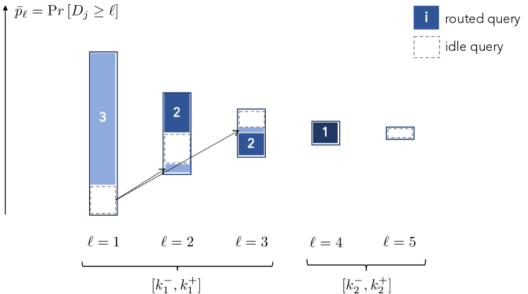
Figure 1: Illustration of TypeRound in stage $t=3$ for an example with $L=5$, $\bar{p}_{\ell}=\frac{1}{2^{\ell-1}}$ for all $\ell\in[L]$, and ${\bf x}_{j}=(\frac{1}{8},\frac{3}{8},\frac{7}{8},\frac{1}{4},0)$. The $y$-axis visualizes the probabilistic space, including the disjointedness of events (by interpreting the arrow). In stage $t=3$, there are $L-t=2$ combined queries left, e.g., the first combined query is formed by the “probabilistically disjoint” idle queries of index $\ell\in[3]$. The random routing $\pi^{t}$ is either $(3,2,\perp,1,\perp)$ or $(3,\perp,2,1,\perp)$ with equal probability 0.4, or $(\perp,3,2,1,\perp)$ or $(\perp,2,3,1,\perp)$ with equal probability 0.1.

Base case $\boldsymbol{(t=0)}$.

Initially, we have $\pi^{0}(\ell)=\perp$ for all $\ell\in[L]$. The property of Matching Marginals is clearly satisfied since none of the queries have been routed and ${\mathbb{E}}[\sum_{\ell=1}^{L}\bar{p}_{\ell}\cdot\mathbbm{1}\{\pi^{t}(\ell)=i\}]=0$ for all $i\in[n]$. Here, we define the segments as the singletons $k^{-}_{\ell}=k^{+}_{\ell}=\ell$ for all $\ell\in[L]$. Property (a) of Combined Queries is straightforward since ${\rm Pr}[\pi^{0}(\ell)=\perp]=1$ and property (b) holds because $D_{j}^{0}=D_{j}$. Finally, the property of Separated Routing trivially holds as $t=0$.

Inductive case $\boldsymbol{(t+1\geq 1)}$.

Suppose that $(D^{t}_{j},\pi^{t})$ satisfy properties 1-3. We define $\pi^{t+1}$ by greedily routing a certain idle query to resource $t+1$. One crucial question is whether we can even find an idle query of type $j$ sufficiently frequently to be routed to resource $t+1$ with probability $x^{*}_{t+1,j}$. The next claim answers this question in the affirmative.

Claim 1

${\rm Pr}[D^{t}_{j}\geq 1]\geq x^{*}_{t+1,j}$.

The proof of Claim 1 is deferred to Section 3.3. Now, we define $\ell^{*}$ as the maximum index $\ell\in[L-t]$ such that ${\rm Pr}[D^{t}_{j}\geq\ell]\geq x^{*}_{t+1,j}$. Since $t\leq n-1\leq L-1$, we have $L-t\geq 1$ and thus the index $\ell^{*}$ is always well-defined by Claim 1. Intuitively, we will choose either the $\ell^{*}$-th or $\ell^{*}+1$-th idle query to be routed to resource $t+1$. In a sense, our approach chooses the latest-arriving combined queries that can satisfy resource $t+1$ with probability $x^{*}_{i,j}$; by the definition of $\ell^{*}$, all combined queries after $\ell^{*}+1$ do not arrive frequently enough.

To formalize these notions, let $\lambda^{*}=\frac{x^{*}_{t+1,j}-{\rm Pr}[D^{t}_{j}\geq\ell^{*}+1]}{{\rm Pr}[D^{t}_{j}\geq\ell^{*}]-{\rm Pr}[D^{t}_{j}\geq\ell^{*}+1]}$ and let $B_{t+1}$ be a Bernoulli random variable with probability of success $\lambda^{*}$, sampled independently from the arrival process and $\pi^{t}$. Additionally, we let $k_{\ell^{*}}$ denote the index $k\in[k_{\ell^{*}}^{-},k_{\ell^{*}}^{+}]$ for which $\pi^{t}(k)=\perp$, and $k_{\ell^{*}+1}$ respectively denote the index $k\in[k_{\ell^{*}+1}^{-},k_{\ell^{*}+1}^{+}]$ for which $\pi^{t}(k)=\perp$, with both indices being uniquely defined due to item (a) of the Combined Queries property. With these definitions at hand, we specify the random routing $\pi^{t+1}$ as follows:

$$\pi^{t+1}(k)=\begin{dcases}t+1&\text{if }k=k_{\ell^{*}}\text{ and }B_{t+1}=1\ ,\\ t+1&\text{if }k=k_{\ell^{*}+1}\text{ and }B_{t+1}=0\ ,\\ \pi^{t}(k)&\text{otherwise. }\end{dcases}$$ (17)

As stated by equation (17), $\pi^{t+1}$ and $\pi^{t}$ coincide for all queries except for one, which is routed to $t+1$. This query is either the $\ell^{*}$-th or the $\ell^{*}+1$-th idle query depending on the outcome of $B_{t+1}$. Note that in the case where $\ell^{*}+1=L-t+1$, the corresponding routing has a probability of zero by the definition $\lambda^{*}$.

In the remainder of the proof, we verify that properties 1-3 are satisfied by $\pi^{t+1}$.

Property of Matching Marginals.

Clearly, none of the resources $i=t+2,t+3,\ldots,n$ are satisfied by $\pi^{t+1}$ by equation (17) as well as property 1 with respect to $\pi^{t}$. Thus, for all $i\geq t+2$,

$${\mathbb{E}}\left[\sum_{\ell=1}^{L}\bar{p}_{\ell}\cdot\mathbbm{1}\{\pi^{t+1}(\ell)=i\}\right]=0$$

Moreover, for each resource $i=1,\ldots,t$, equation (17) implies that $\{\pi^{t+1}(\ell)=i\}=\{\pi^{t}(\ell)=i\}$. It immediately follows that

$${\mathbb{E}}\left[\sum_{\ell=1}^{L}\bar{p}_{\ell}\cdot\mathbbm{1}\{\pi^{t+1}(\ell)=i\}\right]={\mathbb{E}}\left[\sum_{\ell=1}^{L}\bar{p}_{\ell}\cdot\mathbbm{1}\{\pi^{t}(\ell)=i\}\right]=x^{*}_{i,j}\ ,$$

where the last equality follows from property 1 with respect to $\pi^{t}$. It remains to establish a similar inequality with respect to resource $t+1$:

$${\mathbb{E}}\left[\sum_{\ell=1}^{L}\bar{p}_{\ell}\cdot\mathbbm{1}\{\pi^{t+1}(\ell)=t+1\}\right]$$

$$= {\mathbb{E}}\left[\sum_{\ell=1}^{L}\bar{p}_{\ell}\cdot\mathbbm{1}\{\ell=k_{\ell^{*}}\}\cdot\mathbbm{1}\{B_{t+1}=1\}\right]+{\mathbb{E}}\left[\sum_{\ell=1}^{L}\bar{p}_{\ell}\cdot\mathbbm{1}\{k_{\ell^{*}+1}==\ell\}\cdot\mathbbm{1}\{B_{t+1}=0\}\right]$$

$$= {\rm Pr}\left[B_{t+1}=1\right]\cdot{\mathbb{E}}\left[\sum_{\ell=1}^{L}\bar{p}_{\ell}\cdot\mathbbm{1}\{k_{\ell^{*}}=\ell\}\right]+{\rm Pr}\left[B_{t+1}=0\right]\cdot{\mathbb{E}}\left[\sum_{\ell=1}^{L}\bar{p}_{\ell}\cdot\mathbbm{1}\{k_{\ell^{*}+1}=\ell\}\right]$$

$$= \lambda^{*}\cdot{\mathbb{E}}\left[\sum_{\ell=1}^{L}\bar{p}_{\ell}\cdot\mathbbm{1}\{k_{\ell^{*}}=\ell\}\right]+(1-\lambda^{*})\cdot{\mathbb{E}}\left[\sum_{\ell=1}^{L}\bar{p}_{\ell}\cdot\mathbbm{1}\{k_{\ell^{*}+1}=\ell\}\right]$$

$$= \lambda^{*}\cdot{\mathbb{E}}\left[\sum_{\ell=k^{-}_{\ell^{*}}}^{k^{+}_{\ell^{*}}}\mathbbm{1}\{D_{j}\geq\ell\}\cdot\mathbbm{1}\{\pi^{t}(\ell)=\perp\}\right]+(1-\lambda^{*})\cdot{\mathbb{E}}\left[\sum_{\ell=k^{-}_{\ell^{*}+1}}^{k^{+}_{\ell^{*}+1}}\mathbbm{1}\{D_{j}\geq\ell\}\cdot\mathbbm{1}\{\pi^{t}(\ell)=\perp\}\right]$$

$$= \lambda^{*}\cdot{\rm Pr}\left[D_{j}^{t}\geq\ell^{*}\right]+(1-\lambda^{*})\cdot{\rm Pr}\left[D_{j}^{t}\geq\ell^{*}\right]$$

$$= x^{*}_{i,j}\ ,$$

where the first equation proceeds from (17). The second equation holds since the Bernoulli outcome is independent of $\pi^{t}$. The fourth equality proceeds from the fact that $D_{j}$ is independent of $\pi^{t}$ and the fact that $\mathbbm{1}\{k_{\ell^{*}}=\ell\}=\mathbbm{1}\{\pi^{t}(\ell)=\perp\}$ for each $\ell\in[k_{\ell^{*}}^{-},k_{\ell^{*}}^{+}]$, and otherwise $\mathbbm{1}\{k_{\ell^{*}+}=\ell\}=0$ for each $\ell\notin[k_{\ell^{*}}^{-},k_{\ell^{*}}^{+}]$. The fifth equality follows from property 2(b) with respect to $\pi^{t}$. The last equality proceeds by plugging the definition of $\lambda^{*}$.

Property of Combined Queries (a).

We construct a new partition of $[L]$ in stage $t+1$ by merging the intervals $[k^{-}_{\ell^{*}},k^{+}_{\ell^{*}}]$ and $[k^{-}_{\ell^{*}+1},k^{+}_{\ell^{*}+1}]$ and keeping all other intervals unchanged. Specifically, define $k^{-^{\prime}}_{\ell}=k^{-}_{\ell}$ and $k^{+^{\prime}}_{\ell}=k^{+}_{\ell}$ for every $\ell\in[\ell^{*}-1]$. Define $k^{-^{\prime}}_{\ell}=k^{-^{\prime}}_{\ell+1}$ and $k^{+^{\prime}}_{\ell}=k^{+}_{\ell+1}$ for every $\ell\in[\ell^{*}+1,L-t-1]$. Finally, define $k^{-^{\prime}}_{\ell^{*}}=k^{-}_{\ell^{*}}$ and $k^{+^{\prime}}_{\ell^{*}}=k^{+}_{\ell^{*}+1}$. Clearly, the intervals $([k^{-^{\prime}}_{\ell},k^{+^{\prime}}_{\ell}])_{\ell\in[L-t-1]}$ form a partition of $L$ into $L-t-1$ elements. For every $k\in[k^{+^{\prime}}_{\ell^{*}-1}]$, we have $\{\pi^{t+1}(k)=\perp\}=\{\pi^{t}(k)=\perp\}$ since the routings of the $k^{+^{\prime}}_{\ell^{*}-1}=k^{+}_{\ell^{*}-1}$ first queries are unchanged by equation (17). Similarly, for every $k\in[k^{-^{\prime}}_{\ell^{*}+1},k^{+^{\prime}}_{L-t-1}]$, we have $\{\pi^{t+1}(k)=\perp\}=\{\pi^{t}(k)=\perp\}$ since the routing of the queries of rank $k^{-^{\prime}}_{\ell^{*}+1}=k^{-}_{\ell^{*}+2},\ldots,k^{+^{\prime}}_{L-t-1}=k^{+}_{L-t-}$ is unchanged by equation (17). Consequently, property 2(a) for $\pi^{t}$ implies that for all $\ell\in[L-t-1]\setminus\{\ell^{*}\}$, the events $\{\pi^{t+1}(k_{\ell}^{-^{\prime}})=\perp\},\{\pi^{t+1}(k_{\ell}^{-^{\prime}}+1)=\perp\},\ldots,\{\pi^{t+1}(k_{\ell}^{+^{\prime}})=\perp\}$ are disjoint and their union has probability 1. It remains to show that property (2a) holds with respect to the $\ell^{*}$-th segment.

For this purpose, for every $k\in[k^{-}_{\ell^{*}},k^{+}_{\ell^{*}}]$, we note that $\{\pi^{t+1}(k)=\perp\}=\{k_{\ell^{*}}=k\}\cap\{B_{t+1}=0\}$. Indeed, we have $\{\pi^{t+1}(k)=\perp\}\subseteq\{\pi^{t}(k)=\perp\}$ by equation (17). Moreover, $k_{\ell^{*}}$ is the index of the unique idle query in $[k^{-}_{\ell^{*}},k^{+}_{\ell^{*}}]$ with respect to $\pi^{t}$; this arriving query is routed in $\pi^{t+1}$ to resource $t+1$ if and only if $B_{t+1}=1$ as indicated by equation  (17). By a similar reasoning, for every $k\in[k^{-}_{\ell^{*}+1},k^{+}_{\ell^{*}+1}]$, we have $\{\pi^{t+1}(k)=\perp\}=\{k_{\ell^{*}+1}=k\}\cap\{B_{t+1}=1\}$. Using the fact that $\{B_{t+1}=0\}$ and $\{B_{t+1}=1\}$ are disjoint, we infer that the events $\{\pi^{t+1}(k_{\ell^{*}}^{-})=\perp\},\ldots,\{\pi^{t+1}(k_{\ell}^{+})=\perp\},\ldots,\{\pi^{t+1}(k_{\ell^{*}+1}^{-})=\perp\},\ldots,\{\pi^{t+1}(k_{\ell^{*}+1}^{+})=\perp\}$ are disjoint, as precisely stated by property (2a) with the further observation that $k_{\ell^{*}}^{-^{\prime}}=k_{\ell^{*}}^{-}$ and $k_{\ell^{*}}^{+^{\prime}}=k_{\ell^{*}+1}^{+}$. Now, to show that the probabilities of these events sum-up to one, we note that

$$\sum_{k=k_{\ell^{*}}^{-^{\prime}}}^{k_{\ell^{*}}^{+^{\prime}}}{\rm Pr}\left[\pi^{t+1}(k)=\perp\right]$$

$$\quad=\sum_{k=k_{\ell^{*}}^{-}}^{k_{\ell^{*}}^{+}}{\rm Pr}\left[\pi^{t+1}(k)=\perp\right]+\sum_{k=k_{\ell^{*}+1}^{-}}^{k_{\ell^{*}+1}^{+}}{\rm Pr}\left[\pi^{t+1}(k)=\perp\right]$$

$$\quad=\sum_{k=k_{\ell^{*}}^{-}}^{k_{\ell^{*}}^{+}}{\rm Pr}\left[k_{\ell^{*}}=k,B_{t+1}=0\right]+\sum_{k=k_{\ell^{*}+1}^{-}}^{k_{\ell^{*}+1}^{+}}{\rm Pr}\left[k_{\ell^{*}+1}=k,B_{t+1}=1\right]$$

$$\quad=\sum_{k=k_{\ell^{*}}^{-}}^{k_{\ell^{*}}^{+}}{\rm Pr}\left[k_{\ell^{*}}=k\right]\cdot{\rm Pr}\left[B_{t+1}=0\right]+\sum_{k=k_{\ell^{*}+1}^{-}}^{k_{\ell^{*}+1}^{+}}{\rm Pr}\left[k_{\ell^{*}+1}=k\right]\cdot{\rm Pr}\left[B_{t+1}=1\right]$$

$$\quad={\rm Pr}\left[k_{\ell^{*}}\in[k_{\ell^{*}}^{-},k_{\ell^{*}}^{+}]\right]\cdot{\rm Pr}\left[B_{t+1}=0\right]+{\rm Pr}\left[k_{\ell^{*}+1}\in[k_{\ell^{*}+1}^{-},k_{\ell^{*}+1}^{+}]\right]\cdot{\rm Pr}\left[B_{t+1}=1\right]$$

$$\quad=1\ ,$$

where the third equality holds since $B_{t+1}$ is independent of $(D^{t}_{j},\pi^{t})$ by construction and $k_{\ell^{*}}$ and $k_{\ell^{*}+1}$ are measurable functions of $(D^{t}_{j},\pi^{t})$, thereby implying that $B_{t+1}$ is independent of both $k_{\ell^{*}}$ and $k_{\ell^{*}+1}$. The last equality holds since ${\rm Pr}\left[k_{\ell}\in[k_{\ell}^{-},k_{\ell}^{+}]\right]=1$ for all $\ell\in[L-t]$ by property 2(a) with respect to $\pi^{t}$.

Property of Combined Queries (b).

By construction of the partition $([k^{-^{\prime}}_{\ell},k^{+^{\prime}}_{\ell}])_{\ell\in[L-t-1]}$ and property 2(a) for $\pi^{t}$, the $\ell$-th idle query is precisely the unique $k\in[k^{-^{\prime}}_{\ell},k^{+^{\prime}}_{\ell}]$ such that $\pi^{t+1}(k)=\perp$; this query actually arrives if and only if $D_{j}\geq k$. It immediately follows that

$$\left\{D^{t+1}_{j}\geq\ell\right\}=\bigcup_{k=k^{-^{\prime}}_{\ell}}^{k^{+^{\prime}}_{\ell}}\left\{\pi^{t+1}(k)=\perp\right\}\cap\left\{D_{j}\geq k\right\}\ ,$$

which corresponds to property 2(b).

Property of Separated Routing.

To establish property 3, we first consider a resource $i\in[t]$. Due to equation (17), we know that $\pi^{t}(k)=i$ implies that $\pi^{t+1}(k)=i$ for all $k\in[L]$. Moreover, by property 3 for $\pi^{t}$, there exists $\ell_{1}\in[L-t]$ such that ${\rm Pr}[i\in\pi^{t}\langle[k^{-}_{\ell_{1}},k^{+}_{\ell_{1}}]\rangle]=1$. Since the partition $([k^{-}_{\ell},k^{+}_{\ell}])_{\ell\in[L-t]}$ is obtained from the partition $([k^{-^{\prime}}_{\ell},k^{+^{\prime}}_{\ell}])_{\ell\in[L-t-1]}$ by merging two consecutive intervals, it follows that there exists $\ell_{2}\in[L-t-1]$ such that $[k^{-}_{\ell_{1}},k^{+}_{\ell_{1}}]\subseteq[k^{-^{\prime}}_{\ell_{2}},k^{+^{\prime}}_{\ell_{2}}]$. Combining these observations, we have

$${\rm Pr}\left[i\in\pi^{t+1}\langle[k^{-^{\prime}}_{\ell_{2}},k^{+^{\prime}}_{\ell_{2}}]\rangle\right]\geq{\rm Pr}\left[i\in\pi^{t}\langle[k^{-^{\prime}}_{\ell_{2}},k^{+^{\prime}}_{\ell_{2}}]\rangle\right]\geq{\rm Pr}\left[i\in\pi^{t}\langle[k^{-}_{\ell_{1}},k^{+}_{\ell_{1}}]\rangle\right]=1\ .$$

Now, we consider the resource $i=t+1$. Based on equation (17), we have

$${\rm Pr}\left[i\in\pi^{t+1}\langle[k^{-^{\prime}}_{\ell^{*}},k^{+^{\prime}}_{\ell^{*}}]\rangle\right]$$

$$\quad={\rm Pr}\left[t+1\in\pi^{t+1}\langle[k^{-}_{\ell^{*}},k^{+}_{\ell^{*}+1}]\rangle\right]$$

$$\quad={\rm Pr}\left[B_{t+1}=1\right]\cdot{\rm Pr}\left[\perp\in\pi^{t}\langle[k^{-}_{\ell^{*}},k^{+}_{\ell^{*}}]\rangle\right]+{\rm Pr}\left[B_{t+1}=0\right]\cdot{\rm Pr}\left[\perp\in\pi^{t}\langle[k^{-}_{\ell^{*}+1},k^{+}_{\ell^{*}}+1]\rangle\right]$$

$$\quad={\rm Pr}\left[B_{t+1}=1\right]+{\rm Pr}\left[B_{t+1}=0\right]$$

$$\quad=1\ ,$$

where the first equality follows from the fact that $k^{-^{\prime}}_{\ell^{*}}=k^{-}_{\ell^{*}}$ and $k^{+^{\prime}}_{\ell^{*}}=k^{+}_{\ell^{*}+1}$. The next equality proceeds from equation (17), noting that $B_{t+1}$ is independent of $\pi^{t}$. The third equality holds due to property 2(a) with respect to $\pi^{t}$.

3.3 Proof of Claim 1 from the TypeRound Scheme

First, observe that property (3) implies that there exists a subset of resources $S\subseteq[t-1]$ such that $\pi^{t}\langle[k^{+}_{1}]\rangle=S\cup\{\perp\}$ with probability $1$. Moreover, property (2a) implies that $|S|=k_{1}^{+}-1$.

Next, we define the random routing $\tilde{\pi}$ by routing the first idle combined query under $\pi^{t}$ to resource $t+1$. Namely, we have $\tilde{\pi}(\ell)=t+1$ if $\ell\in[k^{-}_{1},k^{+}_{1}]$ and $\pi^{t}(\ell)=\perp$, otherwise $\tilde{\pi}(\ell)=\pi^{t}(\ell)$. By properties (1) and (2a), $\tilde{\pi}$ is a well-defined random routing and resource $t+1$ appears in the random permutation $\tilde{\pi}$ with probability 1. In particular, we have $\tilde{\pi}\langle[k^{+}_{1}]\rangle=S\cup\{t+1\}$ with probability $1$.

Now, suppose for contradiction that ${\rm Pr}[D^{t}_{j}\geq 1]<x^{*}_{t+1,j}$. Because the first idle combined query under $\pi^{t}$ is routed to resource $t+1$, property (2b) together with our construction of $\tilde{\pi}$ yield

$$\sum_{\ell=1}^{k^{+}_{1}}\bar{p}_{\ell}\cdot{\rm Pr}\left[\tilde{\pi}(\ell)=t+1\right]={\rm Pr}\left[D^{t}_{j}\geq 1\right]<x^{*}_{t+1,j}\ .$$ (18)

Moreover, properties 1 and 3 imply that, for every $i\in S$,

$$\sum_{\ell=1}^{k^{+}_{1}}\bar{p}_{\ell}\cdot{\rm Pr}\left[\tilde{\pi}(\ell)=i\right]=x^{*}_{i,j}\ .$$ (19)

We infer that

$${\mathbb{E}}\left[\min\left\{D_{j},k^{+}_{1}\right\}\right] = \sum_{\ell=1}^{k^{+}_{1}}\bar{p}_{\ell}$$

$$= \sum_{\ell=1}^{k^{+}_{1}}\bar{p}_{\ell}\cdot\left(\sum_{i\in S\cup\{t+1\}}{\rm Pr}\left[\tilde{\pi}(\ell)=i\right]\right)$$

$$< \sum_{i\in S\cup\{t+1\}}x^{*}_{i,j}\ ,$$

where the second equality follows from the fact that $\{\tilde{\pi}(\ell):\ell\in[k^{+}_{1}]\}=S\cup\{t+1\}$ with probability $1$. The last inequality holds by (18) and (19). We obtain a contradiction in that ${\bf x}^{*}$ violates constraint (12) of $\mathsf{LP}^{\mathsf{trunc}}(\cdot)$, completing the proof.

3.4 Step 2: Threshold-based assignments

In step 2, we consider each resource $i\in[n]$ in turn and construct a corresponding instance of the prophet inequality problem. For all $j\in[m]$, we define $X_{i,j}\in\{0,r_{i,j}\}$ as the two-outcome random variable that takes the value $r_{i,j}$ if one type-$j$ query is ultimately routed to resource $i$ and $0$ otherwise, i.e., $X_{i,j}=r_{i,j}\cdot\sum_{\ell=1}^{L}\mathbbm{1}\{D_{j}\geq\ell\}\mathbbm{1}\{\pi_{j}(\ell)=i\}$. Now, consider the single-unit prophet inequality problem with respect to the collection of random rewards $\{X_{i,j}\}_{j\in[m]}$. The latter random variables are mutually independent owing to the independence property of the demand vector $(D_{j})_{j\in[m]}$ by definition of Indep and the fact that the permutations $(\pi_{j})_{j\in[m]}$ are drawn independently from each other. In this context, we can write the fluid relaxation LP as a benchmark for the performance of online policies:

$$\mathsf{LP}_{i}=\max\ \ \ \ \ \sum_{j=1}^{m}r_{i,j}y_{j}$$

s.t. $$\sum_{j=1}^{m}y_{j}\leq 1$$ (20)

$$y_{j}\leq{\rm Pr}\left[X_{i,j}=r_{i,j}\right] \forall j\in[m]$$

$$y_{j}\geq 0 \forall j\in[m]\ .$$

It is known that a policy which sets a certain fixed threshold $\tau\in{\mathbb{R}}$ can be $\frac{1}{2}$-competitive relative to $\mathsf{LP}_{i}$. To elaborate, such a policy collects the first reward larger than or equal to $\tau$, if any, and otherwise the payoff is zero if no reward meets this criterion by the end of the horizon. Its random payoff $R^{\tau}_{i}$ is the smallest reward in $\{X_{i,j}\}_{j\in[m]}$ larger than or equal to $\tau$, if one exists, and otherwise $R^{\tau}_{i}=0$. In this context, the following result can be found in Chawla et al. (2010, Thm 24).

Theorem (Chawla et al. (2010)) For $\tau^{*}_{i}=\frac{\mathsf{LP}_{i}}{2}$, we have ${{\mathbb{E}}[R^{\tau^{*}_{i}}_{i}]}\geq\frac{1}{2}\cdot\mathsf{LP}_{i}$.

Our algorithm leverages this result by setting the threshold of each resource $i\in[n]$ precisely as $\tau^{*}_{i}$.

Completing the proof of Theorem 2.4.

To conclude, we establish the desired performance guarantee in Theorem 2.4 by combining the properties entailed by steps 1 and 2 of our randomized matching policy. We take the perspective of each resource $i\in[n]$ in isolation. We make two crucial observations about our reduction to the prophet inequality problem.

First, we can relate the payoff of the threshold policy in the prophet inequality instance to the rewards collected by our policy in the original instance ${\cal I}$. For that, let $R_{i}({\bf D},\sigma)$ be the random variable describing the contribution of resource $i$ to the total rewards of our policy when $\sigma$ and ${\bf D}$ realize. We establish in Appendix 6.5 that $R_{i}({\bf D},\sigma)$ is lower bounded by the payoff $R^{\tau_{i}^{*}}_{i}$ of the $\tau^{*}_{i}$-threshold policy.

Claim 2

$R_{i}({\bf D},\sigma)\geq R^{\tau_{i}^{*}}_{i}$.

Second, by Lemma 3.2, we know that one query of type $j$ is routed to each resource $i$ with probability exactly $x^{*}_{i,j}$. Based on our definition of the rewards $\{X_{i,j}\}_{j\in[m]}$, it follows that $\sum_{j=1}^{m}{\rm Pr}[X_{i,j}=r_{i,j}]=\sum_{j=1}^{m}x^{*}_{i,j}\leq 1$, where this inequality is a direct consequence of constraint (7). This crucially implies that an optimal solution of $\mathsf{LP}_{i}$ takes a simple form, where all constraints except possibly (20) are binding. This structural property can be otherwise expressed as follows.

Claim 3

$\mathsf{LP}_{i}=\sum_{j=1}^{m}{\rm Pr}[X_{i,j}=r_{i,j}]=\sum_{j=1}^{m}r_{i,j}x^{*}_{i,j}$.

Putting everything together, we have

$$\mathsf{ALG}({\cal I}) = {\mathbb{E}}_{{\bf D}}\left[\inf_{\sigma\in{\cal S}({\bf D})}\mathsf{ALG}\left({\bf D},\sigma\right)\right]$$

$$= {\mathbb{E}}_{{\bf D}}\left[\inf_{\sigma\in{\cal S}({\bf D})}\sum_{i=1}^{n}R_{i}({\bf D},\sigma)\right]$$

$$\geq \sum_{i=1}^{n}{\mathbb{E}}_{{\bf D}}\left[R^{\tau_{i}^{*}}_{i}\right]$$

$$\geq \frac{1}{2}\cdot\sum_{i=1}^{n}\mathsf{LP}_{i}$$

$$\geq \frac{1}{2}\cdot\sum_{i=1}^{n}\sum_{j=1}^{m}r_{i,j}x^{*}_{i,j}$$

$$= \frac{1}{2}\cdot\mathsf{LP}^{\mathsf{trunc}}({\cal I})\ ,$$

where the first inequality holds by Claim 2, the second inequality follows from the prophet inequality attributed to Chawla et al. (2010), and the last one comes from Claim 3. This concludes our proof that our policy is $\frac{1}{2}$-competitive.

4 Concluding Remarks

This paper develops a new framework to formulate online stochastic matching problems. We study specific models, Indep and Correl, that provide natural extensions of the Poisson arrival process and capture distinct correlation patterns. Quite surprisingly, we are able identify best-possible competitive (or approximate) algorithms for these settings. In both cases, our approach crucially requires tightening of the fluid LP which often constitutes a valid benchmark for existing models. This illustrates (at least theoretically) our hypothesis that under correlated, high-variance demand, the design of matching policies should not be premised on a fluid approximation which uses only the expectation of demand. Future research could possibly sharpen our understanding of the performance of policies informed by different underlying problem relaxations. Another direction is to extend our framework by identifying other distributions of demand vectors and arrival orders that admit constant-factor approximations.

Although our numerical analysis on JD.com data shows the limitations of standard online matching models, it does not in any way affirm the superiority of the Indep or Correl models, nor does it support the assumptions of adversarial or random-order arrivals. Doing so would require an extensive statistical analysis that is beyond the scope of this work, and that differs from the objectives of our modeling framework. Indeed, estimating a demand process in practice might require identifying stochastic processes that best fits the data of arrival sequences. This task is likely to be context-specific (e.g., ridesharing versus retail). By contrast, our framework is nonparametric in that the distribution of the demand vector ${\bf D}=(D_{j})_{j\in[m]}$ under Indep or Correl can be arbitrary along certain dimensions (i.e., marginal demand or total demand). Data-driven estimation is possible by constructing an empirical estimate of the distributions from observed samples of the demand vector in the data. Our framework simply combines such demand distributions implied by the data with the age-old adversarial and random-order arrival models from the online matching literature, leading to a wealth of new models that can be studied in the future.

The authors thank Rajan Udwani for sharing the insights in Remark 3.1, Daniela Saban for providing comments on an early verison of the paper that significantly improved the presentation, and Kangning Wang for pointing us to the reference Alijani et al. (2020).

E-Companion

5 Comparing Means to Variances on JD.com data

Recall that a consequence of the serial independence assumption, standard in online stochastic matching, is that $\mathrm{Var}(D_{j})\leq\mathbb{E}[D_{j}]$ for the demands of all types $j$. We empirically check whether this assumption is valid using the publicly available data set from JD.com (Shen et al. 2020).

Problem description.

The online matching problem faced by JD.com consists of dynamically dispatching customer orders containing a SKU (from different locations) to different fulfillment centers (that still have inventory of that SKU) over time. Higher rewards are obtained when orders are dispatched to nearby distribution centers, resulting in an edge-weighted online matching problem. The time horizon represents the duration between inventory replenishments, which we assume to be one week. A demand $D_{j}$ is then the total amount that customers ordered in a week, with the type $j$ referring to a particular SKU and a particular location.

Data and findings.

We empirically determine the weekly realizations of $D_{j}$ from the JD.com data, which consists of orders throughout China from a single product category in March 2018. Each week yields a sample of $D_{j}$ for every (SKU, location)-combination $j$. We evaluate the empirical mean and variance of these samples for each combination of the 40 highest-selling SKUs and 40 largest locations (determined by the destination fulfillment center in China). In the resultant scatter-plot Figure 2, we visualize the log-ratio of empirical variance to empirical mean (y-axis) as a function of the empirical mean (x-axis).

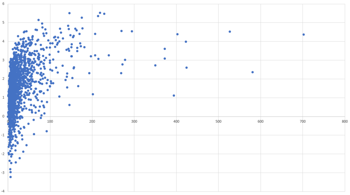
Figure 2: Each of the 1600 dots represents a (SKU, location)-combination $j$. The $x$-coordinate is the empirical mean weekly demand for that SKU from that location, and the $y$-coordinate is the natural logarithm of the ratio of empirical variance to empirical mean. The property $\mathrm{Var}(D_{j})\leq\mathbb{E}[D_{j}]$ would imply that the corresponding dot is below the $y=0$ line with high probability.

If the samples of $D_{j}$ were truly drawn from a distribution such that $\mathrm{Var}(D_{j})\leq\mathbb{E}[D_{j}]$, then for a majority of types $j$, the corresponding dot should lie below the $y=0$ line. However, as displayed in Figure 2, this is not the case and the empirical variance is greater than the empirical mean for most types, often by orders of magnitude. Only for a minority of (SKU, location)-combinations is the empirical variance lower than the empirical mean. This suggests that standard online stochastic matching models might not accurately reflect the stochastic demand faced by JD.com, leading to misrepresentation of the dynamic fulfillment problem. Counter-intuitively, the standard assumption $\mathrm{Var}(D_{j})\leq\mathbb{E}[D_{j}]$ appears to hold for SKUs $j$ with small demand rather than large demand.

Details and limitations of our analysis.

When choosing the 40 highest-selling SKUs, we eliminate any SKU that had zero demand on any day because they may suggest an inventory stockout. However, we otherwise assume that enough inventory was available and that the observed sales coincides with the true demand. Naturally this heuristic does not fully resolve the issue of data censoring. Second, we remove from the data the first day of sales, which we found to be three times higher than an average day due to promotions. Other than such pre-processing steps, we did not control for price fluctuations that may cause additional demand variation.

The variance of SKU-level demands can be explained by several factors, including ones that can be anticipated by the retailer. It is plausible that after controlling for contextual factors like promotions, price changes, and calendar events, the “unexplained” variance in the demand is lower than what is observed in Figure 2. However, it seems unlikely that JD.com could construct SKU-level demand forecasts that reverse the phenomenon observed in Figure 2. Because the dynamic fulfillment decisions are coupled across SKUs in the same product category, our findings remain relevant as long as a non-negligible fraction of SKUs exhibits high-variance demand. Generally speaking, our observations are consistent with the hypothesis that orders are positively correlated over time, i.e., arrivals of a certain type beget more arrivals of the same type, and thus, that more accurate forecasts can be obtained based on intra-week information updates (as implied by our models).

6 Additional proofs from Section 2.1

6.1 Proof of Proposition 2.1

We first present construction (i). Consider a family of instances parametrized by $\varepsilon\in(0,1)$. Each instance comprises a single resource $i=1$ with capacity $k_{i}=1$ and a single query type $j=1$ with the normalized reward $r_{1,1}=1$. The demand random variable $D_{1}$ takes two values $\{0,\lceil\frac{1}{\varepsilon}\rceil\}$ with probabilities ${\rm Pr}[D_{1}=0]=1-\varepsilon$ and ${\rm Pr}[D_{1}=\frac{1}{\varepsilon}\rceil]=\varepsilon$. Because ${\mathbb{E}}[D_{1}]=1$, it is clear that $\mathsf{LP}({\cal I})=1$. However, the single resource can be matched to at most one query, which only occurs with probability ${\rm Pr}[D_{1}>0]={\rm Pr}[D_{1}=\frac{1}{\varepsilon}\rceil]=\varepsilon$. We have just shown that $\frac{\mathsf{OFF}({\cal I})}{\mathsf{LP}({\cal I})}=\varepsilon$, which proves part (i) of Proposition 2.1.

We now present our construction for part (ii). Fix a large $n$, and let $k_{i}=1$ for all $i\in[n]$. Let $m=1$, and let $r_{i,1}=0$ unless $i=1$, in which case $r_{1,1}=1$. Let $D_{1}$ take the value $n$ with probability $\frac{1}{n}$, and take the value 0 with the residual probability $1-\frac{1}{n}$. Note that $D_{1}$ is indeed no greater than $\sum_{i=1}^{n}k_{i}=n$ with probability 1. It is feasible in the fluid relaxation LP to set $x_{1,1}=1$, yielding an objective value $1$. Meanwhile, any algorithm can match query type 1 to resource type 1 with probability at most $\frac{1}{n}$ (when $D_{1}=n$). Therefore, we have shown that $\frac{\mathsf{OFF}(\mathcal{I})}{\mathsf{LP}(\mathcal{I})}=\frac{1}{n}$, where $n$ can be arbitrarily large, thereby completing the proof of Proposition 2.1.

6.2 Separation oracle for $\mathsf{LP}^{\mathsf{trunc}}({\cal I})$

We briefly present an algorithm that provides a separation oracle for constraints (8) and runs in time $O(mn\bar{K})$ where $\bar{K}=\sum_{i=1}^{n}k_{i}$.

Algorithm.

Our separation oracle takes an input a vector ${\bf x}=(x_{i,j})_{i\in[n],j\in[m]}$ and either certifies that all constraints (8) are satisfied or it returns a separating hyperplane, corresponding to one of the violated constraints.

The algorithm enumerates all combinations of a type $j\in[m]$ with an integer $k\in[\bar{K}]$. For each such pair $(j,k)$, we construct the following instance of the integral knapsack problem: find $S\subseteq[n]$ that maximises $\sum_{i\in S}x_{i,j}$ subject to $\sum_{i\in S}k_{i}\leq K$. This problem can be easily solved via dynamic programming in time $O(Kn)$. Let $S^{*}_{j,k}$ be an optimal solution. Our algorithm checks whether or not $\sum_{i\in S^{*}_{j,k}}x_{i,j}\leq{\mathbb{E}}[\min\{D_{j},k\}]$. If this inequality is met, our algorithm continues on to the next instantiation of the parameters $(j,k)$, otherwise it stops and returns constraint (8) with $S=S^{*}_{j,k}$.

Properties.

We briefly argue that the preceding algorithm effectively provides a separation oracle for constraints (8). Suppose that there exists $S\subseteq[n]$ and $j\in[m]$ such that $\sum_{i\in S^{*}_{j,k}}x_{i,j}>{\mathbb{E}}[\min\{D_{j},\sum_{i\in S}k_{i}\}]$. Then, for the pair $(j,k)$ with $k=\sum_{i\in S}k_{i}$, our algorithm identifies the subset $S^{*}_{j,k}$ such that

$$\sum_{i\in S^{*}_{j,k}}x_{i,j}\geq\sum_{i\in S}x_{i,j}>{\mathbb{E}}\left[\min\left\{D_{j},\sum_{i\in S}k_{i}\right\}\right]={\mathbb{E}}\left[\min\left\{D_{j},K\right\}\right]\geq{\mathbb{E}}\left[\min\left\{D_{j},\sum_{i\in S^{*}_{j,k}}k_{i}\right\}\right]\ ,$$

where the first inequality follows the optimality of $S^{*}_{j,k}$, the next one holds because we assume that constraint is violated, and the last inequality proceeds from the budget constraint of the knapsack instance. All-in-all, our algorithm returns a constraint of $\mathsf{LP}^{\mathsf{trunc}}({\cal I})$ violated by the vector ${\bf x}$.

Conversely, suppose that all constraints (8) are met by ${\bf x}$. Then, for all pairs $(j,k)$ examined by our algorithm, we have

$$\sum_{i\in S^{*}_{j,k}}x_{i,j}\leq{\mathbb{E}}\left[\min\left\{D_{j},\sum_{i\in S^{*}_{j,k}}k_{i}\right\}\right]\leq{\mathbb{E}}\left[\min\left\{D_{j},\sum_{i\in S^{*}_{j,k}}k_{i}\right\}\right]\ .$$

In turn, this implies that our algorithm returns that all constraints (8) are satisfied.

6.3 Proof of Lemma 2.3

To show that $\mathsf{OFF}({\cal I})\leq\mathsf{LP}^{\mathsf{trunc}}({\cal I})$, we represent the offline-optimum as the output of a certain exponentially sized linear program. The offline benchmark solves a max-weight matching problem with respect to any specific realization ${\bf d}$ of the demand ${\bf D}$. Letting $\bar{d}=\{{\bf d}:{\rm Pr}[{\bf D}={\bf d}>0]$ be the support of ${\bf D}$, the offline benchmark can be formulated as:

$$\mathsf{OFF}({\cal I})=\ \ \max\ \ \sum_{d\in\bar{{\bf d}}}{\rm Pr}\left[{\bf D}={\bf d}\right]\cdot\left(\sum_{i=1}^{n}\sum_{j=1}^{m}r_{i,j}x^{{\bf d}}_{i,j}\right)$$

s.t. $$\sum_{j=1}^{m}x^{{\bf d}}_{i,j}\leq k_{i} \forall i\in[n],\forall{\bf d}\in\bar{{\bf d}}$$ (21)

$$\sum_{i=1}^{n}x^{{\bf d}}_{i,j}\leq{\bf d}_{j} \forall j\in[m],\forall{\bf d}\in\bar{{\bf d}}$$ (22)

$$x^{{\bf d}}_{i,j}\geq 0 \forall i\in[n],\forall j\in[m],\forall{\bf d}\in\bar{{\bf d}}\ .$$

By combining inequalities (21) and (22), Fix a feasible solution $(x^{{\bf d}}_{i,j})_{i\in[n],j\in[m],{\bf d}\in\bar{{\bf d}}}$ of the above LP. For all ${\bf d}\in\bar{{\bf d}}$, $j\in[m]$, and $S\subseteq[n]$, we have $\sum_{i\in S}x^{{\bf d}}_{i,j}\leq\sum_{i=1}^{n}x^{{\bf d}}_{i,j}\leq{\bf d}_{j}$ based on constraint (22). By summing inequalities (21) over all $i\in S$, we infer that $\sum_{i\in S}x^{{\bf d}}_{i,j}\leq\sum_{i\in S}\sum_{j=1}^{m}x^{{\bf d}}_{i,j}\leq\sum_{i\in S}k_{i}$. By combining these inequalities, we infer that any solution of the offline LP must satisfy $\sum_{i\in S}x^{{\bf d}}_{i,j}\leq\min\{{\bf d}_{j},\sum_{i\in S}k_{i}\}$. Now, we consider the vector $(x_{i,j})_{i\in[n],j\in[m]}$ with $x_{i,j}=\sum_{{\bf d}\in\bar{{\bf d}}}{\rm Pr}[{\bf D}={\bf d}]\cdot x^{{\bf d}}_{i,j}$, obtained as the weighted sum of the offline assignment variables. Based on the previous observation, for each $S\subseteq[n]$ and $j\in[m]$, we have

$$\sum_{i\in S}x_{i,j}=\sum_{{\bf d}\in\bar{{\bf d}}}{\rm Pr}[{\bf D}={\bf d}]\cdot\left(\sum_{i\in S}x^{{\bf d}}_{i,j}\right)\leq\sum_{{\bf d}\in\bar{{\bf d}}}{\rm Pr}[{\bf D}={\bf d}]\cdot\min\left\{{\bf d}_{j},\sum_{i\in S}k_{i}\right\}={\mathbb{E}}\left[\min\left\{D_{j},\sum_{i\in S}k_{i}\right\}\right]\ ,$$

which indicates that $(x_{i,j})_{i\in[n],j\in[m]}$ satisfies constraint (8) of $\mathsf{LP}^{\mathsf{trunc}}({\cal I})$. It is straightforward to verify that all other constraints of $\mathsf{LP}^{\mathsf{trunc}}({\cal I})$ are also met by $(x_{i,j})_{i\in[n],j\in[m]}$. By exploiting this mapping, it follows that $\mathsf{OFF}({\cal I})\leq\mathsf{LP}^{\mathsf{trunc}}({\cal I})$.

6.4 Proof of Proposition 2.5

Let $n=1$ and fix any starting capacity $k_{1}$, which can be arbitrarily large. There are $m=2$ query types, with $r_{1,1}=1$ and $r_{1,2}=1/\varepsilon$, for some small $\varepsilon>0$. The demand vector ${\bf D}$ realizes to $(k_{1},k_{1})$ with probability $\varepsilon$, and $(k_{1},0)$ with the residual probability $1-\varepsilon$. The arrival order is such that all queries of type 2 arrive after all queries of type 1.

The offline optimum collects reward $\frac{k_{1}}{\varepsilon}$ when $D_{2}=k_{1}$, and $k_{1}$ when $D_{2}=0$, which implies in expectation that

$$\mathsf{OFF}(\mathcal{I})=\varepsilon\cdot\frac{k_{1}}{\varepsilon}+(1-\varepsilon)\cdot k_{1}=(2-\varepsilon)k_{1}\ .$$

Meanwhile, any online algorithm does not know whether $D_{2}$ will be $k_{1}$ or 0 during the first $k_{1}$ arrivals, corresponding to all queries of type 1. Suppose it accepts $k$ queries of type 1, for some $k\leq k_{1}$. Then, it will collect expected rewards $k+\varepsilon\cdot(k_{1}-k)\cdot\frac{1}{\varepsilon}=k_{1}$. Therefore, $\mathsf{ALG}(\mathcal{I})\leq k_{1}=\frac{1}{2-\varepsilon}\cdot\mathsf{OPT}(\mathcal{I})$, and taking the limit $\varepsilon\to 0$ completes the proof.

6.5 Proof of Claim 2

Suppose that resource $i$ is matched to some query $(j,\ell)$. Hence, the corresponding reward random variable $X_{i,j}$ satisfies

$$X_{i,j}=r_{i,j}\cdot\left(\sum_{\ell^{\prime}=1}^{L}\mathbbm{1}\{\pi_{j}(\ell^{\prime})=i\wedge D_{j}\geq\ell^{\prime}\}\right)=r_{i,j}\geq\tau^{*}_{i}\ ,$$

where the second equality holds because $\pi_{j}(\ell)=i$ and $D_{j}\geq\ell$, noting that since $(j,\ell)$ is routed to $i$ and $\pi_{j}$ being a permutation, we have $\pi_{j}(\ell^{\prime})\neq i$ for all $\ell^{\prime}\neq\ell$ . The last inequality follows from the threshold rule used in step 2. The fact that $X_{i,j}\geq\tau^{*}_{i}$ immediately implies that $R_{i}({\bf D},\sigma)\geq R_{i}^{\tau^{*}}$, recalling that $R^{\tau^{*}_{i}}_{i}$ is the smallest reward in $\{X_{i,j}\}_{j\in[m]}$ larger or equal to $\tau^{*}_{i}$.

It remains to consider the case where resource $i$ is unmatched, meaning that $R_{i}({\bf D},\sigma)=0$. Conditional on this event, it suffices to show that $X_{i,j}<\tau^{*}_{i}$ for all $j\in[m]$, which clearly implies that the $\tau^{*}_{i}$-threshold policy does not collect any reward, and thus, $R_{i}({\bf D},\sigma)=R_{i}^{\tau^{*}}=0$. Suppose ad absurdum that there exist $j\in[m]$ such that $X_{i,j}\geq\tau^{*}_{i}$. By the definition of $X_{i,j}$, there must exist $\ell\in[L]$ for which $\pi_{j}(\ell)=i$ and $D_{j}\geq\ell$. This means that at least $\ell$ queries of type $j$ arrive and query $(j,\ell)$ is then routed to resource $i$. Because $r_{i,j}=X_{i,j}\geq\tau^{*}_{i}$, it follows that our policy should assign resource $i$ to query $(j,\ell)$ if it is still available. This contradict the initial hypothesis $R_{i}({\bf D},\sigma)=0$.

7 Additional proofs from Section 2.2

7.1 Proof of Lemma 2.7

Fix any online algorithm, and on a sample path of its execution, let $X^{t}_{i,j}\in\{0,1\}$ be the indicator random variable for a query of type $j$ being matched to resource $i$ in time step $t$. Let $Q^{t}_{j}\in\{0,1\}$ be the indicator random variable for a query at step $t$ having type $j$, where we note that $Q^{t}:=\sum_{j}Q^{t}_{j}\leq 1$, with $Q^{t}=0$ whenever the total demand $D$ is less than $t$.

On any sample path, the reward collected by the algorithm is $\sum_{i,j,t}r_{i,j}X^{t}_{i,j}$. Meanwhile, the constraint $\sum_{j,t}X^{t}_{i,j}\leq k_{i}$ must be satisfied for every resource $i$, since $i$ can be matched at most $k_{i}$ times; and the constraint $\sum_{i}X^{t}_{i,j}\leq Q^{t}_{j}$ must be satisfied for every $j$ and $T$, since a query at step $t$ of type $j$ can be matched to at most one $i$, and only if $Q^{t}_{j}=1$. Taking an expectation over only the sample paths where $Q_{T}=1$, i.e., paths where $D$ realized to its maximum value of $T$, we have

$$\sum_{j=1}^{m}\sum_{t=1}^{T}{\mathbb{E}}\left[\left.X^{t}_{i,j}\right|Q_{T}=1\right]\leq k_{i} \forall i\in[n]$$

$$\sum_{i=1}^{n}{\mathbb{E}}\left[\left.X^{t}_{i,j}\right|Q_{T}=1\right]\leq p_{t,j} \forall j\in[m],\forall t\in[T]$$

noting that $\mathbb{E}[Q^{t}_{j}]=p_{t,j}$. Now, we derive for any $i$, $j$, and $t$ that

$${\mathbb{E}}\left[\left.X^{t}_{i,j}\right|Q_{T}=1\right]\leavevmode\nobreak\ =\leavevmode\nobreak\ {\mathbb{E}}\left[\left.X^{t}_{i,j}\right|Q_{t}=1\right]\leavevmode\nobreak\ =\leavevmode\nobreak\ \frac{\mathbb{E}[X^{t}_{i,j}Q_{t}]}{\mathbb{E}[Q_{t}]}\leavevmode\nobreak\ =\leavevmode\nobreak\ \frac{\mathbb{E}[X^{t}_{i,j}]}{\Pr[D\geq t]}\ ,$$ (23)

where the first equality holds because an online algorithm’s decision $X^{t}_{i,j}$ at time $t$ cannot distinguish between $Q_{t}=1$ and the stronger future event that $Q_{T}=1$, and the final equality holds because $X^{t}_{i,j}=1$ implies $Q_{t}=1$ while $\mathbb{E}[Q_{t}]=\Pr[D\geq t]$ by definition. Applying (23), the expected reward collected by the algorithm is $\mathbb{E}[\sum_{i,j,t}r_{i,j}X^{t}_{i,j}]=\sum_{i,j,t}r_{i,j}\mathbb{E}[X^{t}_{i,j}|Q_{T}=1]\cdot\Pr[D\geq t]$.

Letting $y^{t}_{i,j}=\mathbb{E}[X^{t}_{i,j}|Q_{T}=1]$ for all $i$, $t$, and $j$, we see that this forms a feasible solution to $\mathsf{LP}^{\mathsf{cond}}(\mathcal{I})$ with objective value equal to the expected reward collected by the algorithm. Since any online algorithm corresponds to such a feasible solution to $\mathsf{LP}^{\mathsf{cond}}(\mathcal{I})$, the optimal objective value of $\mathsf{LP}^{\mathsf{cond}}(\mathcal{I})$ can be no less than the expected reward of any online algorithm, thereby completing the proof of Lemma 2.7.

7.2 Proof of Theorems 2.8 and 2.11

We prove the more general Theorem 2.11. Theorem 2.8 is then implied because $\gamma^{*}_{k}\geq\gamma^{*}_{1}=1/2$.

Our algorithm works as follows. First we solve $\mathsf{LP}^{\mathsf{cond}}(\mathcal{I})$, and hereafter let $y^{t}_{i,j}$ refer to the variables in an optimal solution. For all $t=1,\ldots,T$, conditional on $D\geq t$ and a query of type $j$ arriving, the algorithm routes this query to each resource $i\in[n]$ with probability $y^{t}_{i,j}/p_{t,j}$ (rejecting the query with probability $1-\sum_{i}y^{t}_{i,j}/p_{t,j}$), which defines a valid probability distribution by LP constraint (12). This randomized routing is independent over time. If a query gets routed to a resource, it could still get rejected by that resource, in which case it does not get rerouted.

Each resource $i$ takes the following accept/reject policy for queries that get routed to it. It imagines that $D=T$, i.e., queries will arrive in all time steps $t=1,\ldots,T$. In time step $t$, it will get routed a query independently with probability $y^{t}_{i}:=\sum_{j=1}^{m}y^{t}_{i,j}$; in this case we say that query $t$ is active. The expected number of active queries is $\sum_{t=1}^{T}y^{t}_{i}$, which is at most the capacity $k_{i}$ by LP constraint (11). The policy can only accept active queries while being constrained by the capacity $k_{i}$. Moreover, we would like to ensure that in all time steps $t$, an active query is accepted with conditional probability at least $\gamma$, for a constant $\gamma\in[0,1]$ as large as possible. Fortunately, this is exactly the Online Contention Resolution Scheme (OCRS) problem (in the fictional world where $D=T$), and for any value of $k_{i}$, the optimal accept/reject policy and constant $\gamma=\gamma^{*}_{k_{i}}$ is known (Jiang et al. 2022). We run this OCRS separately for each resource $i$ in the true world (where $D$ might stop before $T$), which completes the specification of the algorithm.

To analyze our algorithm in the true world, we consider the following coupling with the fictional world. The true world follows exactly the fictional world and the algorithm operates without knowing the difference, except that any reward it collects in time steps $t>D$ are not accounted for, where $D$ is the realization of the stochastic horizon in the true world. We analyze the probability that the algorithm matches a query of type $j$ to resource $i$ at time $t$ in the fictional world, in which time step $t$ is guaranteed to occur. That query will draw type $j$ with probability $p^{t}_{i,j}$, and conditional on this, gets routed to resource $i$ with probability $y^{t}_{i,j}/p_{t,j}$. Conditional on getting routed to $i$, since all of these events are independent, the query will get accepted with probability at least $\gamma^{*}_{k_{i}}$, from the promise made by the OCRS. We note that this promise was made for a generic active query at time $t$ looking at its type, so it holds irrespective of the type $j$. This shows that in the fictional world, $j$ gets matched to $i$ at time $t$ with probability at least $p^{t}_{i,j}\cdot y^{t}_{i,j}/p_{t,j}\cdot\gamma^{*}_{k_{i}}=\gamma^{*}_{k_{i}}y^{t}_{i,j}$. It follows that the probability of the reward $r_{i,j}$ being collected in time step $t$ in the true world is at least ${\rm Pr}[D\geq t]\cdot\gamma^{*}_{k_{i}}y^{t}_{i,j}$.

Since the preceding analysis holds for all $i\in[n],j\in[m],t\in[T]$, we have

$$\mathsf{ALG}(\mathcal{I}) \geq\sum_{i=1}^{n}\gamma^{*}_{k_{i}}\cdot\sum_{j=1}^{m}\sum_{t=1}^{T}r_{i,j}\cdot\Pr[D\geq t]\cdot y^{t}_{i,j}$$

$$\geq\gamma^{*}_{k}\cdot\sum_{i=1}^{n}\sum_{j=1}^{m}\sum_{t=1}^{T}r_{i,j}\cdot\Pr[D\geq t]\cdot y^{t}_{i,j}$$

$$=\gamma^{*}_{k}\cdot\mathsf{LP}^{\mathsf{cond}}(\mathcal{I})^{\prime},$$

where the second inequality holds because $\gamma^{*}_{k_{i}}$ is increasing in $k_{i}$ and $k_{i}\geq k$, and the equality holds because $(y^{t}_{i,j})_{t,i,j}$ is an optimal solution. This completes the proof of $\mathsf{ALG}(\mathcal{I})/\mathsf{LP}^{\mathsf{cond}}(\mathcal{I})\geq\gamma^{*}_{k}$.

7.3 Proof of Proposition 2.9

Let $n=1$ with $k_{1}=1$. Fix a large $T$ and a small $\varepsilon>0$. Let $D$ be distributed over $\{1,\ldots,T\}$ as follows: for any $t=1,\ldots,T-1$, the survival rate is $\Pr[D>t|D\geq t]=\varepsilon$. Types are defined so that conditional on any time step $t\in[T]$ occurring, the reward for matching with the resource is $1/\varepsilon^{t}$ with probability $\varepsilon$, and $1/\varepsilon^{t-1}$ with probability $1-1/\varepsilon$.

We claim that $\mathsf{OPT}(\mathcal{I})\geq T-O(\varepsilon)$ by considering the following online algorithm. In any time step $t$, it only accepts the query if the reward is the larger realization of $1/\varepsilon^{t}$ (which occurs with probability $\varepsilon$). Such an algorithm will accept a query in time step $t$ if $D\geq t$, which occurs with probability $\varepsilon^{t-1}$; conditional on this, no query is accepted before time step $t$, which occurs with probability $(1-\varepsilon)^{t-1}$. Therefore,

$$\mathsf{ALG}(\mathcal{I}) =\sum_{t=1}^{T}\varepsilon^{t-1}(1-\varepsilon)^{t-1}\varepsilon\cdot\frac{1}{\varepsilon^{t}}$$

$$\geq T\cdot(1-\varepsilon)^{T}\ .$$

Now consider any policy that sets a fixed threshold of $1/\varepsilon^{t}$, for some $t\in\{0,\ldots,T\}$. This policy can only collect reward in at most 2 time steps, $t$ or $t+1$. The maximum reward that can be collected in any time step $t$ (assuming there is available capacity, and accepting either realization $1/\varepsilon^{t}$ or $1/\varepsilon^{t-1}$) is

$$\Pr[D\geq t]\cdot\left(\varepsilon\cdot\frac{1}{\varepsilon^{t}}+(1-\varepsilon)\frac{1}{\varepsilon^{t-1}}\right)=\varepsilon^{t-1}\left(\varepsilon\cdot\frac{1}{\varepsilon^{t}}+(1-\varepsilon)\frac{1}{\varepsilon^{t-1}}\right)\leq 2\ .$$

Therefore, such a policy has expected reward upper-bounded by 4, which is an arbitrarily small fraction of $T\cdot(1-\varepsilon)^{T}$ as $T$ tends to $\infty$ and $\varepsilon$ tends to $0$.

7.4 Proof of Proposition 2.10

Let $n=1$ and $k_{1}=1$. Fix a large integer $N$. Let $m=2$, with the type rewards given by $r_{1,1}=1$ and $r_{1,2}=N^{2}$. Let the distribution for the total demand $D$ be $D=1$ with probability $1-1/N$, and $D=1+N^{2}$ with probability $1/N$. Each query draws an IID type that is 1 with probability $p_{1}:=1-1/N^{3}$ and 2 with probability $p_{2}:=1/N^{3}$.

The following is a feasible solution with respect to $\mathsf{LP}^{\mathsf{cond}}(\mathcal{I})$: set $y^{1}_{1,1}=1-(1+N^{2})/N^{3}<p_{1}$ and $y^{1}_{1,2}=1/N^{3}=p_{2}$; set $y^{t}_{1,1}=0$ and $y^{t}_{1,2}=1/N^{3}$ for $t=2,\ldots,1+N^{2}$. Intuitively, this fractional solution accepts both types of queries when $t=1$, and only accepts queries of type 2 when the time horizon $D$ “survives” past $t=1$. Constraint (12) is satisfied by construction, and constraint (11) can be verified because its left-hand side equals $1-(1+N^{2})/N^{3}+(1+N^{2})\cdot 1/N^{3}=1$. Now, the objective value is

$$1-\frac{1+N^{2}}{N^{3}}+N^{2}\left(\frac{1}{N^{3}}+\Pr[D\geq 2]\cdot N^{2}\cdot\frac{1}{N^{3}}\right) =1-\frac{1}{N^{3}}+N^{2}\left(\frac{1}{N}N^{2}\cdot\frac{1}{N^{3}}\right)$$

$$=2-O\left(\frac{1}{N^{3}}\right)\ .$$

Meanwhile, consider any online algorithm. If its plan is to accept type 1 in time step 1, then its expected reward is $1-1/N^{3}+N^{2}\cdot 1/N^{3}=1+O(1/N)$. On the other hand, if its plan is to reject type 1 in time step 1, then its expected reward is at most $N^{2}\cdot(1+1/N\cdot N^{2})\cdot 1/N^{3}$ which is also $1+O(1/N)$. Taking $N\to\infty$ completes the proof.

References

- Aggarwal et al. (2011) Aggarwal G, Goel G, Karande C, Mehta A (2011) Online vertex-weighted bipartite matching and single-bid budgeted allocations. Proceedings of the twenty-second annual ACM-SIAM symposium on Discrete Algorithms, 1253–1264 (SIAM).
- Alaei et al. (2012a) Alaei S, Fu H, Haghpanah N, Hartline J, Malekian A (2012a) Bayesian optimal auctions via multi-to single-agent reduction. arXiv preprint arXiv:1203.5099 .
- Alaei et al. (2012b) Alaei S, Hajiaghayi M, Liaghat V (2012b) Online prophet-inequality matching with applications to ad allocation. Proceedings of the 13th ACM Conference on Electronic Commerce, 18–35.
- Alijani et al. (2020) Alijani R, Banerjee S, Gollapudi S, Munagala K, Wang K (2020) Predict and match: Prophet inequalities with uncertain supply. Proceedings of the ACM on Measurement and Analysis of Computing Systems 4(1):1–23.
- Asadpour et al. (2020) Asadpour A, Niazadeh R, Saberi A, Shameli A (2020) Sequential submodular maximization and applications to ranking an assortment of products. Chicago Booth Research Paper (20-26).
- Bai et al. (2022) Bai Y, El Housni O, Jin B, Rusmevichientong P, Topaloglu H, Williamson D (2022) Fluid approximations for revenue management under high-variance demand: Good and bad formulations. Available at SSRN .
- Border (1991) Border KC (1991) Implementation of reduced form auctions: A geometric approach. Econometrica: Journal of the Econometric Society 1175–1187.
- Brubach et al. (2016) Brubach B, Sankararaman KA, Srinivasan A, Xu P (2016) New algorithms, better bounds, and a novel model for online stochastic matching. 24th Annual European Symposium on Algorithms (ESA 2016) (Schloss Dagstuhl-Leibniz-Zentrum fuer Informatik).
- Buchbinder et al. (2021) Buchbinder N, Wajc D, et al. (2021) A randomness threshold for online bipartite matching, via lossless online rounding. arXiv preprint arXiv:2106.04863 .
- Chawla et al. (2010) Chawla S, Hartline JD, Malec DL, Sivan B (2010) Multi-parameter mechanism design and sequential posted pricing. Proceedings of the forty-second ACM symposium on Theory of computing, 311–320.
- Ehsani et al. (2018) Ehsani S, Hajiaghayi M, Kesselheim T, Singla S (2018) Prophet secretary for combinatorial auctions and matroids. Proceedings of the twenty-ninth annual acm-siam symposium on discrete algorithms, 700–714 (SIAM).
- Fahrbach et al. (2020) Fahrbach M, Huang Z, Tao R, Zadimoghaddam M (2020) Edge-weighted online bipartite matching. 2020 IEEE 61st Annual Symposium on Foundations of Computer Science (FOCS), 412–423 (IEEE).
- Feldman et al. (2009) Feldman J, Korula N, Mirrokni V, Muthukrishnan S, Pál M (2009) Online ad assignment with free disposal. International workshop on internet and network economics, 374–385 (Springer).
- Gamlath et al. (2019a) Gamlath B, Kale S, Svensson O (2019a) Beating greedy for stochastic bipartite matching. Proceedings of the Thirtieth Annual ACM-SIAM Symposium on Discrete Algorithms, 2841–2854 (SIAM).
- Gamlath et al. (2019b) Gamlath B, Kapralov M, Maggiori A, Svensson O, Wajc D (2019b) Online matching with general arrivals. 2019 IEEE 60th Annual Symposium on Foundations of Computer Science (FOCS), 26–37 (IEEE).
- Gandhi et al. (2006) Gandhi R, Khuller S, Parthasarathy S, Srinivasan A (2006) Dependent rounding and its applications to approximation algorithms. Journal of the ACM (JACM) 53(3):324–360.
- Hall (1987) Hall P (1987) On representatives of subsets. Classic Papers in Combinatorics 58–62.
- Huang and Shu (2021) Huang Z, Shu X (2021) Online stochastic matching, poisson arrivals, and the natural linear program. Proceedings of the 53rd Annual ACM SIGACT Symposium on Theory of Computing, 682–693.
- Huang et al. (2022) Huang Z, Shu X, Yan S (2022) The power of multiple choices in online stochastic matching. arXiv preprint arXiv:2203.02883 .
- Jiang et al. (2022) Jiang J, Ma W, Zhang J (2022) Tight guarantees for multi-unit prophet inequalities and online stochastic knapsack. Proceedings of the 2022 Annual ACM-SIAM Symposium on Discrete Algorithms (SODA), 1221–1246 (SIAM).
- Jin and Williamson (2021) Jin B, Williamson DP (2021) Improved analysis of ranking for online vertex-weighted bipartite matching in the random order model. International Conference on Web and Internet Economics, 207–225 (Springer).
- Karp et al. (1990) Karp RM, Vazirani UV, Vazirani VV (1990) An optimal algorithm for on-line bipartite matching. Proceedings of the twenty-second annual ACM symposium on Theory of computing, 352–358.
- Kesselheim et al. (2013) Kesselheim T, Radke K, Tönnis A, Vöcking B (2013) An optimal online algorithm for weighted bipartite matching and extensions to combinatorial auctions. European symposium on algorithms, 589–600 (Springer).
- Kleinberg and Weinberg (2019) Kleinberg R, Weinberg SM (2019) Matroid prophet inequalities and applications to multi-dimensional mechanism design. Games and Economic Behavior 113:97–115.
- Laub et al. (2015) Laub PJ, Taimre T, Pollett PK (2015) Hawkes processes. arXiv preprint arXiv:1507.02822 .
- Ma and Simchi-Levi (2020) Ma W, Simchi-Levi D (2020) Algorithms for online matching, assortment, and pricing with tight weight-dependent competitive ratios. Operations Research 68(6):1787–1803.
- Mahdian and Yan (2011) Mahdian M, Yan Q (2011) Online bipartite matching with random arrivals: an approach based on strongly factor-revealing lps. Proceedings of the forty-third annual ACM symposium on Theory of computing, 597–606.
- Manshadi et al. (2012) Manshadi VH, Gharan SO, Saberi A (2012) Online stochastic matching: Online actions based on offline statistics. Mathematics of Operations Research 37(4):559–573.
- Mehta (2013) Mehta A (2013) Online matching and ad allocation. Foundations and Trends® in Theoretical Computer Science 8(4):265–368.
- Papadimitriou et al. (2021) Papadimitriou C, Pollner T, Saberi A, Wajc D (2021) Online stochastic max-weight bipartite matching: Beyond prophet inequalities. Proceedings of the 22nd ACM Conference on Economics and Computation, 763–764.
- Samuel-Cahn (1984) Samuel-Cahn E (1984) Comparison of threshold stop rules and maximum for independent nonnegative random variables. the Annals of Probability 1213–1216.
- Shen et al. (2020) Shen M, Tang CS, Wu D, Yuan R, Zhou W (2020) Jd. com: Transaction-level data for the 2020 msom data driven research challenge. Manufacturing & Service Operations Management .
- Simchi-Levi et al. (2005) Simchi-Levi D, Chen X, Bramel J, et al. (2005) The logic of logistics. Theory, algorithms, and applications for logistics and supply chain management .
- Talluri and Van Ryzin (2004) Talluri KT, Van Ryzin G (2004) The theory and practice of revenue management, volume 1 (Springer).