Quasinormal frequencies of the dimensionally reduced BTZ black hole

Abstract

We calculate numerically the quasinormal frequencies of the Klein-Gordon and Dirac fields moving in the two-dimensional dimensionally reduced BTZ black hole. Our work extends results previously published on the damped oscillations of this black hole. First, we compute the quasinormal frequencies of the minimally coupled Klein-Gordon field for a range of the dimensionally reduced BTZ black hole physical parameters that is not previously analyzed. Furthermore we determine, for the first time, the quasinormal frequencies of the Dirac field propagating in the dimensionally reduced BTZ black hole. For the Dirac field we use the Horowitz-Hubeny method and the asymptotic iteration method, while for the Klein-Gordon field the extension of the previous results is based on the asymptotic iteration method. Finally we discuss our main results.

KEYWORDS: Quasinormal frequencies, Klein-Gordon and Dirac fields, 2D dimensionally reduced BTZ black hole, Horowitz-Hubeny method, Asymptotic iteration method

1 Introduction

In the intermediate stage a perturbed black hole relaxes towards equilibrium performing a set of characteristic oscillations called quasinormal modes (QNMs in what follows). These modes are damped and the boundary condition that satisfy near the event horizon is that the perturbation is purely ingoing [1]–[3]. At the asymptotic region the boundary condition that fulfill the QNMs depends on the asymptotic structure of the black hole. For example, for asymptotically anti-de Sitter black holes usually is imposed that the perturbation field goes to zero at the asymptotic region [4]-[9]. The frequencies of the QNMs are complex, the usually known as quasinormal frequencies (QNFs in what follows), and we notice that the real part determines the oscillation frequency, whereas the imaginary part governs the decay rate. It is well known that the QNFs depend on the parameters of the black hole, the properties of the perturbation field, and they do not depend on the initial conditions of the perturbation. Also, these damped modes provide useful information on several characteristics of the black holes, such as the classical stability and the way they interact with the environment. More recently, the QNFs of asymptotically anti-de Sitter black holes have found applications in the framework of the AdS/CFT correspondence, since they are useful to determine the relaxation times in quantum field theories [1]–[3], [6], [10].

Many two-dimensional gravity models have been studied and at the present time we know many exact solutions that represent two-dimensional black holes (2D black holes in what follows). This fact is useful since the theories of two-dimensional gravity allow us to study in more detail some classical and quantum properties of the black holes [11], [12]. For example, for classical fields moving in 2D black holes, their equations of motion simplify and this fact allows us to calculate exactly some properties as the values of their QNFs. Some examples in which it is possible to calculate exactly the QNFs of 2D black holes are given in Refs. [13]–[27], however there are some 2D black holes for which a numerical computation is necessary to determine their QNFs [22], [26].

We notice that several 2D black holes are obtained by making a dimensional reduction to higher dimensional solutions [11], [12]. An example is the dimensional reduction of the BTZ black hole proposed by Achucarro and Ortiz [28]. From the static three-dimensional BTZ black hole they obtain the so-called Jackiw-Teitelboim black hole (JT black hole in what follows). Also, from the rotating three-dimensional BTZ black hole they find the usually known as dimensionally reduced BTZ black hole (DRBTZ black hole in what follows [24]). The properties of these 2D black holes are widely studied [11], [12], [22], [24], [28]. For example, the QNFs of the minimally coupled Klein-Gordon field and the Dirac field propagating in the JT black hole are exactly calculated in Ref.  [22]. In contrast to the three-dimensional BTZ black hole [10], [29], for the minimally coupled Klein-Gordon field moving in the DRBTZ black hole, the solutions to its radial equation are not expanded in terms of hypergeometric functions and a numerical calculation is necessary to determine its QNFs. Thus in Ref.  [22], taking as a basis the Horowitz-Hubeny method [6], they numerically calculate the QNFs of the minimally coupled Klein-Gordon field. Nevertheless, in order to the Horowitz-Hubeny numerical method converges, a restriction on the value of the inner horizon radius was imposed in Ref.  [22].

In this work, our main objective is to extend the results of Ref. [22]. We make this extension in two ways. First, we calculate the QNFs of the minimally coupled Klein-Gordon field for a larger range than in Ref. [22] of the DRBTZ black hole physical parameters. Also our work is an extension of some results previously published in Ref. [24] on the QNFs of the Klein-Gordon field propagating on the DRBTZ black hole and our results extend those of Ref. [25] on the QNFs of a scalar field propagating on the JT black hole. In Refs. [24], [25] they use a modified Klein-Gordon equation. In contrast to [24], [25] and in a similar way to [22], in what follows we calculate the QNFs of a minimally coupled Klein-Gordon field to study the effect on its propagation of the DRBTZ black hole geometry. Furthermore we comment that the QNFs of the minimally coupled Klein-Gordon field are commonly studied in several backgrounds [1]–[3]. Second, in the DRBTZ black hole we numerically compute the QNFs of the Dirac field that were not calculated in the previous references.

Our results allow us to study the following: i) The classical stability under perturbations of the 2D DRBTZ black hole. ii) The response of the DRBTZ black hole to Klein-Gordon and Dirac perturbations. Furthermore, using our results we compare the response of the studied black holes to the minimally coupled Klein-Gordon field and to the generalized Klein-Gordon field, previously examined in Refs. [24], [25]. In a similar way, our results allow us to compare the response of the BTZ black hole and the dimensional reduction proposed by Achucarro-Ortiz. iii) The dependence of the QNFs on the physical parameters of the black hole and the field. Therefore we extend the results of Ref. [22] to analyze whether the dependence on the black hole physical parameters is of the same form for the values that are not previously explored and we calculate the spectrum of QNFs for the Dirac field. For these reasons we think that it is useful to explore the spectrum of QNFs of the 2D DRBTZ black hole.

The rest of this paper is organized as follows. In the following section we give the relevant properties for our work of the DRBTZ black hole. In Sect. 3 we extend the previous results on the QNFs of the minimally coupled Klein-Gordon field propagating in the DRBTZ black hole. In contrast to Ref. [22] that used the Horowitz-Hubeny numerical method [6], in this section our computations are based on the Asymptotic Iteration Method (AIM in what follows) [31]–[33]. This method allows us to analyze a larger range of the DRBTZ black hole physical parameters. In Sect. 4 we present our numerical results on the QNFs of the Dirac field moving in the DRBTZ black hole. For this field, in the computation we use the AIM and Horowitz-Hubeny method, but the first method allows us to explore a larger range of the DRBTZ black hole physical parameters. We discuss our main results in Sect. 5. We describe the main characteristics of the AIM in Appendix A and finally in Appendix B, for the Dirac field propagating in the DRBTZ black hole we expound the mathematical steps to transform its radial equations into a convenient form to use the Horowitz-Hubeny method in the calculation of its QNFs.

2 Dimensionally reduced BTZ black hole

The DRBTZ black hole is a dimensional reduction of the three-dimensional rotating BTZ black hole. This 2D back hole is a solution to the equations of motion for the action [28]

$$S=\int d^{2}x\sqrt{-h}\phi\left(\mathcal{R}+2\Lambda-\frac{J}{2\phi^{4}}\right),$$ (1)

where $h$ is the determinant of the metric, $\mathcal{R}$ is the scalar curvature, $\Lambda=1/l^{2}$ determines the anti-de Sitter radius $l$, $J$ is the angular momentum of the BTZ black hole and $\phi$ is the dilaton field. The line element of the 2D DRBTZ black hole is equal to

$$ds^{2}=f(r)dt^{2}-\frac{dr^{2}}{f(r)},$$ (2)

where

$$f(r)=\frac{r^{2}}{l^{2}}-M+\frac{J^{2}}{4r^{2}},$$ (3)

and the dilaton field is equal to $\phi=r$. This black hole has two horizons located at

$$r_{\pm}^{2}=\frac{l^{2}}{2}\Big{(}M\pm\sqrt{M^{2}-\frac{J^{2}}{l^{2}}}\Big{)},$$ (4)

with $r_{+}$ being the radius of the event horizon and $r_{-}$ being the radius of the inner horizon. Taking into account that

$$M=\frac{r_{+}^{2}+r_{-}^{2}}{l^{2}},\qquad\qquad\qquad J=\frac{2r_{+}r_{-}}{l},$$ (5)

we find that the function (3) can be written as

$$f(r)=\frac{(r^{2}-r_{+}^{2})(r^{2}-r_{-}^{2})}{l^{2}r^{2}}.$$ (6)

In what follows we take units where $l=1$ and we assume that the horizons radii satisfy $r_{+}>r_{-}$. It is convenient to notice that the line element of the JT black hole is obtained from (2) and (3) by taking $J=0$ or equivalently $r_{-}=0$.

3 QNFs of the Klein-Gordon field

Using the Horowitz-Hubeny method, in Ref. [22] are calculated the QNFs of the minimally coupled Klein-Gordon field propagating in the 2D DRBTZ black hole. Nevertheless, in the previous reference, in order to the Horowitz-Hubeny method converges, it is imposed the restriction $r_{+}>2r_{-}$ on the values of the horizons radii. Therefore only for values of the horizons radii fulfilling the previous condition, the QNFs of the Klein-Gordon field are previously calculated. For the 2D DRBTZ black hole, by using the AIM [31]–[33], we can determine the QNFs of the Klein-Gordon field for a larger range of values for the inner horizon radius not satisfying the previous condition that is imposed in the implementation of the Horowitz-Hubeny method of Ref. [22].

In an analogous way to Ref. [22] we define the QNMs of the DRBTZ black hole as the solutions to the equations of motion that satisfy the boundary conditions:

a) They are purely ingoing near the event horizon.

b) They go to zero at the asymptotic region ($r\to\infty$).

As shown in Ref. [23], in a two dimensional spacetime whose line element takes the form

$$ds^{2}=f(r)dt^{2}-\frac{dr^{2}}{g(r)},$$ (7)

where the functions $f$ and $g$ depend only on the $r$ coordinate, the minimally coupled Klein-Gordon equation

$$(\Box+m^{2})\Phi=0,$$ (8)

simplifies to the Schrödinger type equation

$$\frac{d^{2}R}{dr_{*}^{2}}+(\omega^{2}-V)R=0,$$ (9)

when we take $\Phi=R(r)\textrm{exp}{(-i\omega t)}$. In the previous equation $r_{*}$ denotes the tortoise coordinate and in the metric (7) is defined by

$$r_{*}=\int\frac{dr}{\sqrt{fg}}.$$ (10)

The effective potential $V$ is equal to [23]

$$V=m^{2}f.$$ (11)

We notice that for $m=0$ the effective potential (11) goes to zero. Hence, for the minimally coupled Klein-Gordon field in the massless limit the solutions of the radial equation (9) are sinusoidal functions. As a consequence, in what follows we consider that the mass of the Klein-Gordon field is different from zero and in Fig. 1 we show the effective potential (11) for $m=3/2$, $r_{+}=100$ and $r_{-}=80$ ($M=16400$ and $J=16000$). We notice that the effective potential goes to zero at the horizon of the black hole and diverges as $r\to\infty$.

Figure 1: We show the effective potential (11) for the Klein-Gordon field. We take $m=3/2$, $r_{+}=100$ and $r_{-}=80$ ($M=16400$ and $J=16000$).

In the 2D DRBTZ black hole, Eq. (9) takes the form [22]

$$x(1-x)\frac{d^{2}R}{dx^{2}}+\Big{(}1-x-\frac{r_{+}^{2}-r_{-}^{2}}{2}\frac{x}{r_{+}^{2}-xr_{-}^{2}}\Big{)}\frac{dR}{dx}+\Big{(}\frac{\alpha}{x}+\gamma+\frac{\beta}{1-x}\Big{)}R=0,$$ (12)

where

$$\alpha=\frac{\omega^{2}r_{+}^{2}}{4(r_{+}^{2}-r_{-}^{2})^{2}},\quad\gamma=-\frac{\omega^{2}r_{-}^{2}}{4(r_{+}^{2}-r_{-}^{2})^{2}},\quad\beta=-\frac{m^{2}}{4},$$ (13)

and the variable $x$ is defined by

$$x=\frac{r^{2}-r_{+}^{2}}{r^{2}-r_{-}^{2}}.$$ (14)

To satisfy the boundary conditions a) and b) of the QNMs for the 2D DRBTZ black hole, we take the radial function $R$ as

$$R=x^{-i\alpha^{1/2}}(1-x)^{\frac{1}{4}(1+\sqrt{1+4m^{2}})}\chi(x),$$ (15)

to find that the function $\chi$ must be a solution of the differential equation

$$\frac{d^{2}\chi}{dx^{2}}=\lambda_{0}(x)\frac{d\chi}{dx}+s_{0}(x)\chi,$$ (16)

where

$$\lambda_{0}(x) =\frac{2B+Cr_{-}^{2}/r_{+}^{2}}{1-x}+\frac{C(r_{-}^{2}/r_{+}^{2})^{2}x}{(1-x)(1-xr_{-}^{2}/r_{+}^{2})}-\frac{2A+1}{x},$$ (17)

$$s_{0}(x) =\frac{ACr_{-}^{2}/r_{+}^{2}}{x(1-x)(1-xr_{-}^{2}/r_{+}^{2})}+\frac{B(r_{-}^{2}/r_{+}^{2})}{2(1-x)^{2}}-\frac{BC(r_{-}^{2}/r_{+}^{2})^{2}x}{(1-x)^{2}(1-xr_{-}^{2}/r_{+}^{2})}$$

$$-\frac{\alpha+\gamma+\beta-B(2A+1)}{x(1-x)},$$

with the quantities $A$, $B$, and $C$ defined by

$$A=-i\alpha^{1/2},\qquad B=\frac{1}{4}(1+\sqrt{1+4m^{2}}),\qquad C=\frac{r_{+}^{2}-r_{-}^{2}}{2r_{-}^{2}}.$$ (18)

We notice that Eq. (16) has the mathematical form required by the AIM [31]–[33] (see also Appendix A). Hence, in the following section, taking as a basis Eq. (16) and using the AIM, we numerically calculate the QNFs of the minimally coupled Klein-Gordon field moving in the DRBTZ black hole.

3.1 Numerical results

In Ref. [22] are published the QNFs of the minimally coupled Klein-Gordon field propagating in the DRBTZ black hole. In order to the Horowitz-Hubeny method converges, in the previous reference the restriction $r_{+}>2r_{-}$ was imposed. Using the AIM we reproduce the results presented in the previous reference for $r_{+}>2r_{-}$ and in what follows we mainly show the QNFs of the Klein-Gordon field moving in the DRBTZ black hole whose horizons radii satisfy $r_{-}>r_{+}/2$. We note that for the physical configurations for which the two methods work, the produced numerical results are in agreement.

We recall that in the JT black hole an analytical expression for the QNFs of the minimally coupled Klein-Gordon field is known [22]

$$\omega_{KG}=-i\kappa\left(n+\frac{1}{2}+\frac{1}{2}\sqrt{1+4m^{2}}\right),$$ (19)

where $n$ is the mode number and $\kappa=r_{+}$ is the surface gravity of the JT black hole. We notice that the QNFs (19) are purely imaginary and we also comment that for the Klein-Gordon field propagating in the DRBTZ black hole, we numerically obtain purely imaginary QNFs (see also Refs. [22], [24], [25]). Therefore in our figures we plot the imaginary part of the QNFs and in what follows for the Klein-Gordon field we do not make comments on the real part of its QNFs.

(a) $r_{+}=50$, $r_{-}=10$ ($M=2600$, $J=1000$)

(b) $r_{+}=100$, $r_{-}=10$ ($M=10100$, $J=2000$)

(c) $r_{+}=50$, $r_{-}=40$ ($M=4100$, $J=4000$)

(d) $r_{+}=100$, $r_{-}=80$ ($M=16400$, $J=16000$)

Figure 2: We show the first fifty QNFs of the Klein-Gordon field for different values of the horizons. We take $m=3/4$.

$r_{+}$	$r_{-}$	$\kappa$	Linear fit
50	10	48	$-67.222-48.001n$
100	10	99	$-138.715-99.000n$
50	40	18	$-24.566-18.019n$
100	80	36	$-49.091-36.040n$

Table 1: For the first fifty QNFs of the Klein-Gordon field we give the linear fits for the four examples of Fig. 2. We note that this figure shows the dependence of the QNFs on the mode number.

For the Klein-Gordon field, in Fig. 2 we plot the first fifty QNFs for four different combinations of $r_{+}$ and $r_{-}$. For the presented examples, we see that the plots of Fig. 2 show a linear relation between ${\mathbb{I}}{\mathrm{m}}(\omega)$ and $n$. To analyze this behavior in Table 1 we give the linear fits for the four graphs of Fig. 2. In Table 1 we observe that for the linear fit the absolute value of the slope is almost identical with the value of the surface gravity, that for the DRBTZ black hole is given by [28]

$$\kappa=\frac{r_{+}^{2}-r_{-}^{2}}{r_{+}}.$$ (20)

This behavior is similar to the one we deduce from the exact expression for the QNFs of the JT black hole, but for the DRBTZ black hole the slope is not exactly its surface gravity.

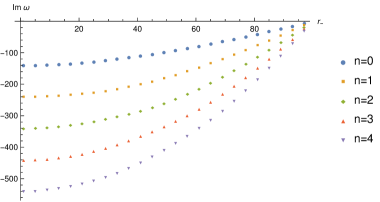
Figure 3: For the Klein-Gordon field of mass $m=3/4$ we show the dependence on the inner horizon radius of the imaginary part for the first five QNFs. We take $r_{+}=100$.

$n$	Quadratic fit
0	$-142.933+0.366r_{-}+0.011r_{-}^{2}$
1	$-241.953+0.039r_{-}+0.024r_{-}^{2}$
2	$-338.972-0.089r_{-}+0.035r_{-}^{2}$
3	$-439.832-0.044r_{-}+0.045r_{-}^{2}$
4	$-539.519-0.050r_{-}+0.055r_{-}^{2}$

Table 2: For the Klein-Gordon field we give the quadratic fits for the QNFs of the first five modes of Fig. 3. We observe that this figure shows the dependence of the QNFs on the inner horizon radius.

$n$	$\omega_{JT}^{a}$	$\omega_{JT}^{q}$	$\mathcal{E}$
0	$-140.139i$	$-142.933i$	1.994 %
1	$-240.139i$	$-241.953i$	0.755 %
2	$-340.139i$	$-338.972i$	0.343 %
3	$-440.139i$	$-439.832i$	0.070 %
4	$-540.139i$	$-539.519i$	0.115 %

Table 3: Based on the quadratic fits of Table 2 we give the predicted values for the QNFs of the Klein-Gordon field moving in the JT black hole ($J=r_{-}=0$) whose QNFs are known analytically [22]. We also show the relative errors.

For the Klein-Gordon field of mass $m=3/4$, in Fig. 3 we show how the QNFs depend on the inner horizon radius for a DRBTZ black hole of event horizon radius $r_{+}=100$. In this figure we observe that the absolute value of the imaginary part of the QNFs decreases as the inner horizon radius increases, that is, the decay time increases as the inner horizon radius increases. The decay time $\tau$ is equal to

$$\tau=\frac{1}{{\lvert\mathbb{I}}{\mathrm{m}}(\omega_{0})\rvert},$$ (21)

where ${\mathbb{I}}{\mathrm{m}}(\omega_{0})$ is the imaginary part of the fundamental mode. Furthermore we observe that for the first five modes the damping decreases as the inner horizon radius increases.

We also see that the variation of the imaginary part of the QNFs with the inner horizon radius can be described by a quadratic relation. For the first five QNFs of Fig.  3 we give the quadratic fits in Table 2. For the QNFs of the Klein-Gordon field propagating in the JT black hole, in Table 3 we show the predicted values when we take as a basis the quadratic fits of Table 2 and compare with the values that produces the exact expression (19). We also give the relative error of the predicted values for the QNFs of the JT black hole. The relative error is defined by

$$\mathcal{E}=\left\lvert\frac{\omega_{JT}^{a}-\omega_{JT}^{q}}{\omega_{JT}^{a}}\right\rvert\times 100\%,$$ (22)

where $\omega_{JT}^{a}$is the value that produces the analytical expression (19) and $\omega_{JT}^{q}$ is the predicted value by the quadratic fit of Table 2. We see that the quadratic fits of Table 2 generate accurate values for the QNFs of the JT black hole.

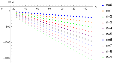
Figure 4: We show the dependence on the event horizon radius of the imaginary part of the first ten QNFs for the Klein-Gordon field of mass $m=3/4$. We take $r_{-}=10$.

$n$	Linear fit
0	$6.053-1.439r_{+}$
1	$6.951-2.447r_{+}$
2	$11.409-3.470r_{+}$
3	$14.316-4.494r_{+}$
4	$17.460-5.508r_{+}$
5	$20.979-6.536r_{+}$
6	$23.926-7.549r_{+}$
7	$27.514-8.576r_{+}$
8	$30.430-9.590r_{+}$
9	$33.981-10.615r_{+}$

Table 4: For the Klein-Gordon field we display the linear fits for the QNFs of the first ten modes of Fig. 4. We notice that this figure shows the dependence on the event horizon radius of the QNFs.

For the DRBTZ black hole of inner horizon radius $r_{-}=10$, in Fig. 4 we show how the first ten QNFs depend on the value of the event horizon radius $r_{+}$. We observe that the imaginary part of the QNFs depends on the value of the event horizon radius in a linear way. Furthermore in Table 4 we write the linear fits for the first ten QNFs presented in Fig. 4. From the expressions of Table 4 we see that the absolute value of the slope increases with the mode number and the value of the slope is approximately equal to $-(n+3/2)$, but we notice that for the first four QNFs the absolute value of the slope is less than $n+3/2$, whereas for the last five modes the absolute value of the slope is greater than $n+3/2$. For $n=4$ the absolute value of the slope is almost equal to $n+3/2$. That is, the slope changes as the mode number varies. This linear behavior is similar to the one we deduce from the exact QNFs of the JT black hole, but for the values of the parameters for our example, the absolute value of the slope for the JT is $n+1/2+\sqrt{13}/4\approx n+1.401$ for all the QNFs (see the formula (19)). Thus for the DRBTZ black hole the absolute value of the slope for the plot ${\mathbb{I}}{\mathrm{m}}(\omega)$ vs $r_{+}$ is greater than the one for the JT black hole and the slope depends on the mode number. Furthermore, from Fig. 4 we get that for fixed inner horizon radius, the decay time decreases as the event horizon radius increases. Also, for the first ten QNMs the damping increases as the event horizon radius increases.

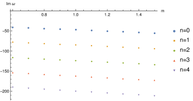
Figure 5: We show the dependence on the field mass of the imaginary part of the QNFs for the Klein-Gordon field. We take $r_{+}=100$ and $r_{-}=80$ ($M=16400$, $J=16000$).

$n$	Linear fit
0	$-30.93-16.08m$
1	$-67.44-17.87m$
2	$-103.83-19.67m$
3	$-140.01-21.55m$
4	$-175.88-23.56m$

Table 5: For the Klein-Gordon field we display the linear fits for the QNFs of the first five modes of Fig. 5. Notice that in this figure we show the dependence of the QNFs on the mass of the field.

In Fig. 5 we show how the imaginary part of the QNFs depends on the mass of the Klein-Gordon field moving in the DRBTZ black hole. We observe that the relation between ${\mathbb{I}}{\mathrm{m}}(\omega)$ and $m$ is linear. In Table 5 we write the linear fits for the first five QNFs of Fig. 5. From the data of this table we deduce that for the linear fits the absolute values of the slopes and the absolute values of the constant terms increase as the mode number increases. Also, from Fig. 5 we obtain that the decay time depends slightly on the mass, in such a way that the decay time decreases as the mass increases.

For the Klein-Gordon field, in each of Figures 3, 4, 5, we notice that the analyzed QNFs behave in a similar way as we change the corresponding physical parameter.

4 QNFs of the Dirac field

Following the usual method [34], we can show that in a bidimensional static spacetime of the form (7) but written as

$$ds^{2}=P^{2}(r)dt^{2}-Q^{2}(r)dr^{2},$$ (23)

where the functions $P$ and $Q$ depend only on $r$, the Dirac equation

$$(i\gamma^{\mu}\nabla_{\mu}-m)\Psi=0,$$ (24)

simplifies to the coupled system of differential equations [26]

$$\frac{1}{P}\partial_{t}\psi_{2}-\frac{1}{Q}\partial_{r}\psi_{2}-\frac{1}{2PQ}\frac{dP}{dr}\psi_{2} =-im\psi_{1},$$

$$\frac{1}{P}\partial_{t}\psi_{1}+\frac{1}{Q}\partial_{r}\psi_{1}+\frac{1}{2PQ}\frac{dP}{dr}\psi_{1} =-im\psi_{2},$$ (25)

when we use the null dyad

$$\hat{e}_{1}^{\;\mu}=\frac{1}{\sqrt{2}}\Big{(}\frac{1}{P},\frac{1}{Q}\Big{)},\qquad\hat{e}_{2}^{\;\mu}=\frac{1}{\sqrt{2}}\Big{(}\frac{1}{P},-\frac{1}{Q}\Big{)},$$ (26)

and the representation of the gamma matrices

$$\gamma_{1}=\frac{1}{\sqrt{2}}\begin{pmatrix}0&2\\ 0&0\end{pmatrix},\quad\gamma_{2}=\frac{1}{\sqrt{2}}\begin{pmatrix}0&0\\ 2&0\end{pmatrix}.$$ (27)

We note that in Eq. (4) the quantities $\psi_{1}$ and $\psi_{2}$ are the components of the spinor $\Psi$, that is,

$$\Psi=\begin{pmatrix}\psi_{1}\\ \psi_{2}\end{pmatrix}.$$ (28)

Taking a harmonic time dependence of the form

$$\psi_{1}(t,r)=R_{1}(r)e^{-i\omega t},\qquad\psi_{2}(t,r)=R_{2}(r)e^{-i\omega t},$$ (29)

we find that the system of equations (4) reduces to

$$\frac{1}{Q}\frac{dR_{2}}{dr}+\frac{i\omega}{P}R_{2}+\frac{1}{2PQ}\frac{dP}{dr}R_{2} =imR_{1},$$

$$\frac{1}{Q}\frac{dR_{1}}{dr}-\frac{i\omega}{P}R_{1}+\frac{1}{2PQ}\frac{dP}{dr}R_{1} =-imR_{2},$$ (30)

from which we obtain decoupled equations for the radial functions $R_{1}$ and $R_{2}$. For 2D spacetimes that fulfill $(PQ)^{2}=1$, for example, the DRBTZ and JT black holes, we find that these decoupled radial equations can be transformed into Schrödinger type equations of the form [26]

$$\frac{dR_{s}}{dr_{*}^{2}}+(\omega^{2}-V_{s})R_{s}=0,\qquad$$ (31)

where $s=1$ ($s=2$) for $R_{1}$ ($R_{2}$) and the effective potentials $V_{s}$ take the form

$$V_{s}=m^{2}f\mp\frac{i\omega}{2}\frac{df}{dr}-\frac{f}{4}\frac{d^{2}f}{dr^{2}}+\frac{1}{16}\Big{(}\frac{df}{dr}\Big{)}^{2},$$ (32)

with the function $f$ defined by $f=P^{2}$, in agreement with the expression (7). In the formula (32) and in what follows the upper (lower) sign corresponds to $s=1$ ($s=2$).

For the Dirac field we notice that the effective potentials (32) are complex. Owing this fact we do not plot these effective potentials. We observe that they are different from the real effective potentials given in Ref. [23], but in the last reference they used a different dyad and a different representation of the gamma matrices to write the Dirac equation. Furthermore, in Ref. [23] is shown that in a two-dimensional spacetime of the form (23), the Dirac equation simplifies to a pair of Schrödinger type equations with effective potentials

$$V_{\pm}=m^{2}f\pm\left(\frac{m}{2}\right)\sqrt{f}\frac{df}{dr},$$ (33)

when $(PQ)^{2}=1$ and $f=P^{2}$, as previously. We note that these effective potentials are real and for the DRBTZ black hole, we plot them in Fig. 6. In a similar way to the effective potential for the Klein-Gordon field (11), the potentials $V_{\pm}$ of the Dirac field go to zero at the horizon of the black hole and diverge as $r\to\infty$.

Figure 6: We show the effective potentials $V_{\pm}$ for the Dirac field moving in the DRBTZ black hole. We take $m=3/4$, $r_{+}=100$, $r_{-}=80$ ($M=16400$, $J=16000$).

We have not been able to find exact solutions to the radial equations (31) in the DRBTZ black hole. Therefore, in what follows, we use numerical methods to find the QNFs of the Dirac field moving in the DRBTZ black hole. In Appendix B we expound the necessary steps to transform the differential equations (31) into an appropriate form to use the Horowitz-Hubeny method [6], but as in Ref. [22], the Horowitz-Hubeny method only works for DRBTZ black holes whose horizons radii satisfy $r_{+}>2r_{-}$. Hence, in this section we transform Eqs. (31) into an appropriate mathematical form to use the AIM [31]–[33] (see also Appendix A), since this numerical procedure works for a larger range of the DRBTZ black hole physical parameters. We first make the ansatz

$$R_{s}=e^{-i(\omega\pm\frac{i\kappa}{2})r_{*}}r^{-(\frac{1}{2}+m)}\tilde{R}_{s}(r),$$ (34)

to consider the boundary conditions a) and b) of the QNMs. In the previous equation, the factor $\textrm{exp}({-i(\omega\pm i\kappa/2)r_{*}})$ takes this form since the effective potentials (32) are different from zero at the event horizon of the DRBTZ black hole. For other fields, for example, the Klein-Gordon field, the effective potentials go to zero at the event horizon and as a consequence, near the event horizon we consider the boundary condition of the QNMs proposing a factor of the form $\textrm{exp}(-i\omega r_{*})$ [6], [22].

From Eqs. (31) we get that the functions $\tilde{R}_{s}$ are solutions to the differential equations

$$\frac{d^{2}\tilde{R}_{s}}{dr^{2}}+F_{s}(r)\frac{d\tilde{R}_{s}}{dr}+G_{s}(r)\tilde{R}_{s}=0,$$ (35)

where

$$F_{s}(r) =\frac{1}{f}\Big{(}\frac{df}{dr}-2i\omega\pm\kappa\Big{)}-\frac{2(\frac{1}{2}+m)}{r},$$ (36)

$$G_{s}(r) =\frac{\kappa^{2}}{4f^{2}}\mp\frac{i\kappa\omega}{f^{2}}-\frac{V_{s}}{f^{2}}-\frac{(\frac{1}{2}+m)}{rf}\Big{(}\frac{df}{dr}-2i\omega\pm\kappa\Big{)}+\frac{(\frac{1}{2}+m)(\frac{3}{2}+m)}{r^{2}}.$$

Making the change of variable

$$u=\frac{r-r_{+}}{r-r_{-}}$$ (37)

we find that Eqs. (35) transform into

$$\frac{d^{2}\tilde{R}_{s}}{du^{2}}=\lambda_{0,s}\frac{d\tilde{R}_{s}}{du}+s_{0,s}\tilde{R}_{s}$$ (38)

where

$$\lambda_{0,s} =-F_{s}(u)\frac{(r_{+}-r_{-})}{(1-u)^{2}}+\frac{2}{1-u},$$

$$s_{0,s} =-\frac{(r_{+}-r_{-})^{2}}{(1-u)^{4}}G_{s}(u).$$ (39)

We note that Eqs. (38) have the mathematical form that is appropriate to use the AIM (see Appendix A) and taking them as a basis we can determine the QNFs of the Dirac field moving in the DRBTZ black hole. Furthermore, we observe that compared to the corresponding formula for the Klein-Gordon field, the previous expressions for $\lambda_{0,s}$ and $s_{0,s}$ are more complicated and to determine the QNFs of the Dirac field the numerical computations will be more difficult. We comment that the QNFs of the Dirac field in the DRBTZ black hole are not previously calculated. To finish this section we notice that our numerical results show that the two effective potentials $V_{s}$ produce the same QNFs for the Dirac field.

4.1 Numerical results

In what follows we give the QNFs of the Dirac field propagating in the DRBTZ black hole. We mention that for the DRBTZ black hole the QNFs of this field were not previously computed in Refs. [22], [24], [25]. For $2r_{-}<r_{+}$ we can use the Horowitz-Hubeny method [6] and the AIM [31]–[33] to calculate the QNFs of the Dirac field moving in the DRBTZ black hole. For the horizons radii for which we can use the two numerical procedures, we find that both methods produce the same QNFs. For horizons radii satisfying $r_{-}>r_{+}/2$ we use only the AIM, due to the Horowitz-Hubeny method does not converge for these values of the radii [22] (see also Appendix B).

We also notice that the QNFs of the Dirac field with mass $m$ propagating in the JT black hole are calculated exactly in Ref. [22] and are equal to

$$\omega_{D}=-i\kappa\left(m+\frac{1}{2}+n\right).$$ (40)

As in the formula (19) for the QNFs of the Klein-Gordon field, in the previous expression, $\kappa=r_{+}$ is the surface gravity of the JT black hole. In the expression (40) we notice that the QNFs of the Dirac field in the JT black hole are purely imaginary and for this field moving in the DRBTZ black hole we numerically obtain purely imaginary QNFs. Therefore, in what follows, for the Dirac field we only discuss the behavior of the imaginary part of its QNFs.

(a) $r_{+}=50$, $r_{-}=10$ ($M=2600$, $J=1000$)

(b) $r_{+}=100$, $r_{-}=10$ ($M=10100$, $J=2000$)

(c) $r_{+}=50$, $r_{-}=40$ ($M=4100$, $J=4000$)

(d) $r_{+}=100$, $r_{-}=80$ ($M=16400$, $J=16000$)

Figure 7: We show the first fifty QNFs of the Dirac field for different values of the horizons. We take $m=3/4$.

$r_{+}$	$r_{-}$	$\kappa$	Linear fit
50	10	48	$-59.961-48.001n$
100	10	99	$-123.718-99.001n$
50	40	18	$-21.708-18.027n$
100	80	36	$-43.502-36.049n$

Table 6: For the Dirac field we display the linear fits for the QNFs of the first fifty modes of Fig. 7. We note that this figure shows the dependence of the QNFs on the mode number.

For the Dirac field and four different configurations of the horizons radii, in Fig. 7 we show how the imaginary part of the QNFs depends on the mode number. We notice that the plots ${\mathbb{I}}{\mathrm{m}}(\omega)$ vs $n$ are linear and in Table 6 we give the linear fits for the four examples that we display in Fig. 7. In an analogous way to the Klein-Gordon field, the slope of the straight line is related to the surface gravity (20) of the DRBTZ black hole, but the value is not exactly the surface gravity, in contrast to the Dirac field moving in the JT black hole for which the slope of the plot ${\mathbb{I}}{\mathrm{m}}(\omega)$ vs $n$ is the surface gravity (see the expression (40)).

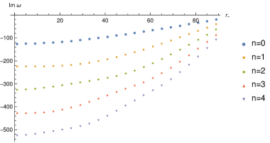
Figure 8: We show the dependence on the inner horizon radius of the imaginary part of the QNFs for the Dirac field of mass $m=3/4$. We take $r_{+}=100$.

$n$	Quadratic fit
0	$-128.269+0.484r_{-}+0.0086r_{-}^{2}$
1	$-226.056-0.257r_{-}+0.027r_{-}^{2}$
2	$-319.193-0.307r_{-}+0.036r_{-}^{2}$
3	$-426.715+0.038r_{-}+0.042r_{-}^{2}$
4	$-523.023-0.089r_{-}+0.053r_{-}^{2}$

Table 7: For the Dirac field we display the quadratic fits for the QNFs of the first five modes of Fig. 8. Notice that in this figure we show the dependence of the QNFs on the inner horizon radius.

$n$	$\omega^{a}_{JT}$	$\omega^{q}_{JT}$	$\mathcal{E}$
0	$-125i$	$-128.269i$	2.615 %
1	$-225i$	$-226.056i$	0.469 %
2	$-325i$	$-319.193i$	1.787 %
3	$-425i$	$-426.715i$	0.403 %
4	$-525i$	$-523.023i$	0.376 %

Table 8: Based on the quadratic fits of Table 7 we give the predicted values for the QNFs of the Dirac field moving in the JT black hole ($J=r_{-}=0$) whose QNFs are known analytically [22]. We also show the relative errors.

For the QNFs of the Dirac field moving in the DRBTZ black hole, in Fig. 8 we display the dependence of the imaginary part on the inner horizon radius of the DRBTZ black hole. We notice that for the first five modes the absolute value of the imaginary part decreases as the inner horizon radius increases. As a consequence, for fixed event horizon radius, as the inner horizon increases the decay time increases. Furthermore we observe that for the first five modes the damping decreases as the inner horizon radius increases.

In Fig. 8 we see that the plots ${\mathbb{I}}{\mathrm{m}}(\omega)$ vs $r_{-}$ can be described by a quadratic relation and in Table 7 we give the quadratic fits for the first five modes of the Fig. 8. Taking as a basis the quadratic fits of Table 7 we can predict the values of the QNFs for the Dirac field moving in the JT black hole. We display the predicted values in Table 8 and compare with the values that produce the analytical expression (40). In this table, for the first five QNFs we also give their relative errors (defined in the formula (22)). We see that the quadratic fits of Table 7 produce accurate values for the QNFs of the Dirac field in the JT black hole, but the relative errors for the QNFs of the Dirac field are larger than those we calculate previously for the first five QNFs of the Klein-Gordon field (see Table 3).

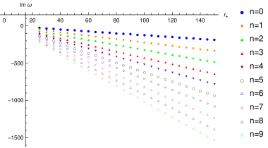
Figure 9: We show the dependence on the event horizon radius of the imaginary part of the QNFs for the Dirac field of mass $m=3/4$. We take $r_{-}=10$.

$n$	Linear fit
0	$6.429-1.289r_{+}$
1	$4.362-2.283r_{+}$
2	$12.799-3.318r_{+}$
3	$12.987-4.350r_{+}$
4	$16.877-5.333r_{+}$
5	$21.227-6.408r_{+}$
6	$22.292-7.365r_{+}$
7	$28.553-8.453r_{+}$
8	$28.138-9.404r_{+}$
9	$35.322-10.491r_{+}$

Table 9: For the Dirac field we display the linear fits for the QNFs of the first ten modes of Fig. 9. We observe that this figure shows how the QNFs depend on the event horizon radius.

For the Dirac field propagating in the DRBTZ black hole with inner horizon radius $r_{-}=10$, in Fig. 9 we show how the imaginary part of the QNFs depends on the event horizon radius. We observe that the plots ${\mathbb{I}}{\mathrm{m}}(\omega)$ vs $r_{+}$ are straight lines in a similar way to the Klein-Gordon field. The linear fits for the graphs of Fig. 9 are given in Table 9. We note in this table that the absolute value of the slope for the straight line increases as the mode number increases, in an analogous way to the Klein-Gordon field previously studied. From the analytical expression (40) for the QNFs of the Dirac field, we deduce that in the JT black hole the slope of similar plots is equal to $-(n+1.25)$ for the same values of the physical parameters. For the first ten modes of the DRBTZ black hole we observe that for the plots ${\mathbb{I}}{\mathrm{m}}(\omega)$ vs $r_{+}$ the absolute values of their slopes are larger than the absolute values of the slopes for the similar plots of the JT black hole. For the Dirac field, from Fig. 9 we also get that for fixed inner horizon radius, the decay time decreases as the event horizon radius increases. Also for the first ten QNMs the damping increases as the event horizon radius increases.

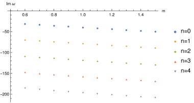
Figure 10: We show the dependence on the field mass of the imaginary part of the QNFs for the Dirac field. We take $r_{+}=100$ and $r_{-}=80$ ($M=16400$, $J=16000$).

$n$	Linear fit
0	$-19.16-20.44m$
1	$-57.62-21.31m$
2	$-95.74-22.36m$
3	$-133.47-23.62m$
4	$-170.63-25.23m$

Table 10: For the Dirac field we display the linear fits for the QNFs of the first five modes of Fig. 10. Notice that in this figure we show how the QNFs depend on the mass of the field.

In Fig. 10 we display how the first five QNFs depend on the mass of the Dirac field. We observe that the graphs ${\mathbb{I}}{\mathrm{m}}(\omega)$ vs $m$ show a linear behavior and in Table 10 we give their linear fits. From these linear fits we deduce that the slopes and constant terms of the straight lines depend on the mode number and their absolute values increase as the mode number increases. This behavior is similar to that of the QNFs for the Klein-Gordon field. From Fig. 10 we obtain that for the Dirac field the decay time depends slightly on its mass, in such a way that the decay time decreases as the mass increases.

For the Dirac field, in each of the Figures 8, 9, 10, we see that the studied QNFs behave in a similar way when we change the physical parameters of the black hole or of the field.

5 Discussion

From the analytical expressions (19) and (40) we get that in the JT black hole the QNFs of the Klein-Gordon and Dirac fields are purely imaginary. In an analogous way, our numerical results show that the QNFs of these two fields are purely imaginary in the DRBTZ black hole. Furthermore we find that for these two fields their QNFs satisfy that ${\mathbb{I}}{\mathrm{m}}(\omega)<0$ and as a consequence their QNMs are stable in the JT and DRBTZ black holes. We notice that for the Dirac field propagating in the DRBTZ black hole its QNFs are not previously calculated and our numerical results show that the two potentials (32) have the same spectrum of QNFs.

For the Klein-Gordon and Dirac fields, from our numerical results we notice that in the DRBTZ black hole, as the inner horizon radius increases the damping of the QNMs decreases, that is, the decay time increases as the inner horizon radius increases. For fixed inner horizon radius, as the event horizon radius increases we find that the damping increases. As a consequence, for both fields, for a given mode number, and for fixed event horizon radius, as we change the inner horizon radius, the more damped QNM occurs for the JT black hole. Furthermore, taking as a basis the linear fits of Tables 4 and 9, for the Klein-Gordon and Dirac fields we find that for $r_{+}>>r_{-}$ the predicted values for the QNFs of the DRBTZ black hole tend to the QNFs of the JT black hole of the same event horizon radius.

For the Klein-Gordon and Dirac fields moving in the DRBTZ black hole, we notice that the effective potentials (11) and (32) are different, nevertheless our numerical results show that the behavior of the QNFs for both fields is similar when we change the physical parameters. We notice that this conclusion follows from the numerical results. Considering the mathematical form of the effective potentials (11) and (32) is not straightforward to deduce that their spectra of QNFs behave in a similar form.

Furthermore, from the analytical expressions (19) and (40) for the QNFs of the JT black hole, we notice that for large mass of the field both expressions behave in the form

$$\omega=-i\kappa\left(n+\frac{1}{2}+m\right).$$ (41)

That is, for the JT black hole, the QNFs of the Klein-Gordon and Dirac fields are almost the same for large values of the field mass. For the DRBTZ black hole our numerical results for the first four modes are shown in Fig. 11, where we plot the quantity $\beta$ defined by

$$\beta=\lvert\omega_{D}-\omega_{KG}\lvert$$ (42)

versus the mass of the field. In the previous expressions $\omega_{D}$ denotes the QNFs of the Dirac field and $\omega_{KG}$ stands for the QNFs of the Klein-Gordon field.

Figure 11: For the DRBTZ black hole with $r_{+}=100$, $r_{-}=80$ ($M=16400$, $J=16000$), and for the first four QNMs, we show the absolute value of the difference of the values for the QNFs of the Dirac and Klein-Gordon fields as the masses of the fields increase.

In Fig. 11 we observe that the quantity $\beta$ decreases as the masses of the fields increase, thus, the difference between the values the QNFs of the Klein-Gordon and Dirac fields decreases as the masses of fields increase. Thus, the QNFs of the DRBTZ black hole behave in a similar way to the QNFs of the JT black hole as the mass of the test field increases.

In the JT black hole, from the analytical expressions (19) and (40) we see that the QNFs of the Klein-Gordon and Dirac fields are different for small values of the mass of the field. In Table 11 we give the QNFs for the first ten modes of the Klein-Gordon and Dirac fields with mass equal to $3/4$ propagating in the DRBTZ black hole with $r_{+}=100$, $r_{-}=80$, and we see that the QNFs of these fields are different, in contrast to some spacetimes for which the QNFs of the Klein-Gordon and Dirac fields are similar [1]–[3]. Thus, for small values of the mass of the field, in the DRBTZ black hole the QNFs of these two fields are different and this behavior is similar to that of the QNFs for the BTZ three-dimensional black hole [10], [29], from which the DRBTZ black hole is a dimensional reduction. Nevertheless, from the data shown in Table 11, we notice that for both fields, as the mode number increases the QNFs of the DRBTZ black hole approach those of the JT black hole with the same surface gravity.

$n$	$\omega_{KG}$ DRBTZ	$\omega_{KG}$ JT	$\omega_{D}$ DRBTZ	$\omega_{D}$ JT
0	-42.980 $i$	-50.450 $i$	-34.499 $i$	-45.000$i$
1	-80.834 $i$	-86.450 $i$	-73.613 $i$	-81.000$i$
2	-118.571 $i$	-122.450 $i$	-112.521 $i$	-117.000$i$
3	-156.151 $i$	-158.450 $i$	-151.205 $i$	-153.000$i$
4	-193.513 $i$	-194.450 $i$	-189.577 $i$	-189.000$i$
5	-230.580 $i$	-230.450 $i$	-227.460 $i$	-225.000$i$
6	-267.270 $i$	-266.450 $i$	-264.538 $i$	-261.000$i$
7	-303.524 $i$	-302.450 $i$	-300.329$i$	-297.000$i$
8	-339.355 $i$	-338.450 $i$	-334.548 $i$	-333.000$i$
9	-374.891 $i$	-374.450 $i$	-368.045$i$	-369.000$i$

Table 11: In the second and fourth columns we give the QNFs of the Klein-Gordon and Dirac fields with mass $m=3/4$ propagating in the DRBTZ black hole with $r_{+}=100$ and $r_{-}=80$ (that is, $\kappa=36$, $M=16400$, and $J=16000$). In the third and fifth columns we show the QNFs of the Klein-Gordon and Dirac fields with mass $m=3/4$ propagating in the JT black hole with surface gravity $\kappa=36$, that is, with radius of the horizon equal to $r_{+}=36$.

In addition, we note the following. For the JT black hole we find that for the massive generalized Klein-Gordon field its QNFs take the form (see the formula (3.13) of Ref. [25] with $\alpha=1$ and $L=1$)

$$\omega_{GKG}=-2ir_{+}\left(n+\frac{1}{2}+\frac{1}{2}\sqrt{1+m^{2}}\right),$$ (43)

and therefore the spacing between consecutive QNFs is equal to

$$\Delta\omega_{GKG}=-i2r_{+}.$$ (44)

From Eq. (19) we get that the spacing for the massive minimally coupled Klein-Gordon field is equal to

$$\Delta\omega_{KG}=-ir_{+},$$ (45)

which is different from the spacing for the generalized Klein-Gordon field studied in Refs. [24], [25].

For the DRBTZ black hole, in Ref. [24] they find that the QNFs of the generalized massive Klein-Gordon field are of two types, the left and the right QNFs given by (see the expressions (4.19a) and (4.19b) of Ref. [24])

$$\omega_{L}=-i(r_{+}-r_{-})(\tilde{\Delta}+2n),\qquad\qquad\omega_{R}=-i(r_{+}+r_{-})(\tilde{\Delta}+2n),$$ (46)

where $m^{2}=\tilde{\Delta}(\tilde{\Delta}-2)$. As a consequence, we get that the spacings between consecutive QNFs are

$$\Delta\omega_{L}=-i2(r_{+}-r_{-}),\qquad\qquad\Delta\omega_{R}=-i2(r_{+}+r_{-}).$$ (47)

Our numerical results point out that the spacing of consecutive QNFs of the minimally coupled Klein-Gordon field is proportional to the surface gravity (20) as the mode number increases and therefore different from the spacings (47) for the generalized massive Klein-Gordon field. Thus, the QNFs of the minimally coupled Klein-Gordon field and of the generalized Klein-Gordon field have some different characteristics in the 2D DRBTZ black hole.

Since the spacing of the QNFs for the minimally coupled Klein-Gordon field in the static (rotating) BTZ black hole is identical [10], [29] to the spacing of the QNFs for the generalized Klein-Gordon field propagating in the 2D JT (DRBTZ) black hole, we can deduce that, for the minimally coupled Klein-Gordon field, the BTZ black hole and the dimensional reduction proposed by Achucarro-Ortiz react in a different way.

Finally, for the 2D DRBTZ black hole, we should investigate the relevance of our numerical results to the discussion of the AdS/CFT correspondence, to the calculation of the microscopic structure of the black hole [25], and to the determination of the spectrum of the event horizon [35], [36], although it is likely that we should extend our computations to the asymptotic regime.

6 Acknowledgments

This work was supported by CONACYT México, SNI México, EDI IPN, COFAA IPN, and Research Project IPN SIP 20221379.

Appendix A Asymptotic iteration method

An useful method to find the eigenvalues of linear second order differential equations is the asymptotic iteration method [31]–[33]. This method works with linear second order differential equations of the form

$$y^{\prime\prime}=\lambda_{0}(x)y^{\prime}+s_{0}(x)y,$$ (48)

where the prime denotes differentiation with respect to the independent variable. Taking advantage of the symmetrical structure of Eq. (48) we find that its first derivative takes a similar mathematical form

$$y^{\prime\prime\prime}=\lambda_{1}(x)y^{\prime}+s_{1}(x)y,$$ (49)

with

$$\lambda_{1}=\lambda_{0}^{\prime}+s_{0}+\lambda_{0}^{2},\quad\textrm{and}\quad s_{1}=s_{0}^{\prime}+s_{0}\lambda_{0}.$$ (50)

In an analogous way we find that the $(n+2)$-th derivative of the function $y$ is equal to [31]–[33]

$$y^{(n+2)}=\lambda_{n}(x)y^{\prime}+s_{n}(x)y,$$ (51)

where

$$\lambda_{n}=\lambda_{n-1}^{\prime}+s_{n-1}+\lambda_{0}\lambda_{n-1},\quad\textrm{and}\quad s_{n}=s_{n-1}^{\prime}+s_{0}\lambda_{n-1}.$$ (52)

The asymptotic aspect of the method imposes that for sufficiently large $n$ the functions $\lambda_{n}$ and $s_{n}$ satisfy [31]–[33]

$$\frac{s_{n}}{\lambda_{n}}=\frac{s_{n-1}}{\lambda_{n-1}}=\alpha$$ (53)

or in an equivalent form

$$s_{n}\lambda_{n-1}-s_{n-1}\lambda_{n}=0.$$ (54)

Solving this equation, usually known as discretization condition, we can find the QNFs of the black hole under study [32], [33].

Nevertheless, the computation of the recurrence relations (52) requires many resources [31]–[33]. Owing this fact, in Ref. [32] is proposed an improved version of the AIM. In this version of the method we expand the functions $\lambda_{n}$ and $s_{n}$ around a convenient point $\xi$, that is,

$$\lambda_{n}(\xi)=\sum^{\infty}_{i=0}c^{i}_{n}(x-\xi)^{i},\qquad\qquad s_{n}(\xi)=\sum^{\infty}_{i=0}d^{i}_{n}(x-\xi)^{i},$$ (55)

to find that the recurrence relations (52) imply that the coefficients $c^{i}_{n}$ and $d^{i}_{n}$ satisfy

$$c^{i}_{n} =(i+1)c^{i+1}_{n-1}+d^{i}_{n-1}+\sum^{i}_{k=0}c^{k}_{0}c^{i-k}_{n-1},$$

$$d^{i}_{n} =(i+1)d^{i+1}_{n-1}+\sum^{i}_{k=0}d^{k}_{0}c^{i-k}_{n-1}.$$ (56)

Furthermore, we get that the discretization condition (54) takes the form

$$d^{0}_{n}c^{0}_{n-1}-d^{0}_{n-1}c^{0}_{n}=0.$$ (57)

Solving this equation for different values of $n$, we numerically obtain the QNFs of the studied black hole [32], [33]. In this work we use this improved formulation of the AIM to find the QNFs of the Klein-Gordon and Dirac fields propagating in the DRBTZ black hole.

Appendix B Horowitz-Hubeny method for the Dirac field

For the Klein-Gordon field moving in the DRBTZ black hole, in Ref. [22] are calculated its QNFs taking as a basis the Horowitz-Hubeny method. Nevertheless a restriction on the values of the horizons radii was imposed, as we previously commented. For the Dirac field we can use the Horowitz-Hubeny method to compute its QNFs in the DRBTZ black hole. In what follows we describe the steps to transform the radial equations (31) into a convenient form to use the Horowitz-Hubeny method [6].

First, to fulfill the boundary condition near the event horizon, we propose that the solutions of Eqs. (31) take the form

$$R_{s}(r)=e^{-i(\omega\pm\frac{i\kappa}{2})r_{*}}U_{s}(r),$$ (58)

to find that the functions $U_{s}$ must satisfy the differential equations

$$f\frac{d^{2}U_{s}}{dr^{2}}+\Big{(}\frac{df}{dr}-2i\omega\pm\kappa\Big{)}\frac{dU_{s}}{dr}+\frac{1}{f}\Big{(}\frac{\kappa^{2}}{4}\mp i\omega\kappa-V_{s}\Big{)}U_{s}=0.$$ (59)

To have an independent variable that changes in a finite interval, following to Horowitz-Hubeny [6], we make the change of variable

$$x=\frac{1}{r},$$ (60)

to get that the radial equations (59) transform into

$$S_{s}(x)\frac{d^{2}U_{s}}{dx^{2}}+\frac{t_{s}(x)}{x-x_{+}}\frac{dU_{s}}{dx}+\frac{u_{s}(x)}{(x-x_{+})^{2}}U_{s}=0,$$ (61)

where the functions $t_{s}(x)$, $u_{s}(x)$, and $S_{s}(x)$ are equal to

$$t_{s}(x) =2x(x^{2}-x_{+}^{2})(x^{2}-x_{-}^{2})^{2}(x+x_{+})+2x^{5}(x+x_{+})(x^{2}-x_{-}^{2})$$

$$-2xx_{+}^{2}x_{-}^{2}(x+x_{+})(x^{2}-x_{-}^{2})+2i\omega x^{2}(x+x_{+})(x^{2}-x_{-}^{2})x_{+}^{2}x_{-}^{2}$$

$$\mp x^{2}x_{+}(x_{-}^{2}-x_{+}^{2})(x+x_{+})(x^{2}-x_{-}^{2}),$$

$$u_{s}(x) =\frac{1}{4}x^{2}x_{+}^{2}(x_{+}^{2}-x_{-}^{2})^{2}\mp i\omega x^{2}x_{+}^{3}x_{-}^{2}(x_{-}^{2}-x_{+}^{2})$$

$$\pm i\omega xx_{+}^{2}x_{-}^{2}(x_{+}^{2}x_{-}^{2}-x^{4})+\frac{5}{4}x^{8}-\frac{3}{2}x^{6}(x_{+}^{2}+x_{-}^{2})+\frac{5}{2}x^{4}x_{+}^{2}x_{-}^{2}$$

$$-\frac{1}{2}x^{2}x_{+}^{2}x_{-}^{2}(x_{+}^{2}+x_{-}^{2})+\frac{1}{4}x_{+}^{4}x_{-}^{4}-m^{2}(x^{2}-x_{+}^{2})(x^{2}-x_{-}^{2})x_{+}^{2}x_{-}^{2},$$

$$S_{s}(x) =x^{2}(x+x_{+})^{2}(x^{2}-x_{-}^{2})^{2}.$$ (62)

In the previous equations we define $x_{+}=1/r_{+}$ and $x_{-}=1/r_{-}$.

As in Ref. [6] we propose that the solutions to Eqs. (61) take the form

$$U_{s}=(x-x_{+})^{\nu_{s}}\sum_{k=0}^{\infty}a_{k,s}(\omega)(x-x_{+})^{k},$$ (63)

but to fulfill the boundary condition of the QNMs near the event horizon we must take $\nu_{s}=0$ [6]. Substituting these simplified forms of the functions $U_{s}$ into Eq. (61), we find that the coefficients $a_{k,s}$ must satisfy the recurrence relations

$$a_{k,s}=-\frac{1}{k(k-1)S_{0,s}+kt_{0,s}}\sum_{n=0}^{k-1}a_{n,s}(n(n-1)S_{k-n,s}+nt_{k-n,s}+u_{k-n,s}),$$ (64)

where $S_{0,s}=S_{s}(x_{+})$, $t_{0,s}=t_{s}(x_{+})$, the coefficients $u_{k,s}$ are given by

$$u_{s}(x)=\sum_{k=0}^{\infty}u_{k,s}(x-x_{+})^{k},$$ (65)

and similar definitions are valid for the coefficients $S_{k,s}$ and $t_{k,s}$.

At the asymptotic region, the boundary condition of the QNMs imposes that as $x\to 0$ ($r\to\infty$) the functions $U_{s}$ go to zero, that is,

$$U_{s}(x=0)=\sum_{k=0}^{\infty}a_{k,s}(\omega)(-x_{+})^{k}=0$$ (66)

and the QNFs of the Dirac field can be calculated by finding the roots of the previous equation when we replace the infinite sum by a finite sum [6].

As for the Klein-Gordon field moving in the DRBTZ black hole, the Horowitz-Hubeny method allows us to calculate the QNFs of the Dirac field when $r_{+}>2r_{-}$. The reason is that the series (63) has a radius of convergence as large as the distance to the nearest singular point. Since the radius of convergence must include the point $x=0$, the distance from the expansion point at $x_{+}$ to the other singularity at $x_{-}$ must be larger than the distance between $x_{+}$ and 0, that is, $x_{-}-x_{+}>x_{+}$, or equivalently $r_{+}>2r_{-}$.

References

- [1] K. D. Kokkotas and B. G. Schmidt, Living Rev. Rel. 2 (1999) 2, [arXiv:gr-qc/9909058].
- [2] R. Konoplya and A. Zhidenko, Rev. Mod. Phys. 83 (2011) 793, [arXiv:1102.4014 [gr-qc]].
- [3] E. Berti, V. Cardoso and A. O. Starinets, Class. Quant. Grav. 26 (2009) 163001, [arXiv:0905.2975 [gr-qc]].
- [4] J. Chan and R. B. Mann, Phys. Rev. D 55, 7546 (1997), [arXiv:gr-qc/9612026 [gr-qc]].
- [5] J. S. F. Chan, R. B. Mann, Phys. Rev. D 59, 064025 (1999).
- [6] G. T. Horowitz and V. E. Hubeny, Phys. Rev. D 62, 024027 (2000), [hep-th/9909056].
- [7] S. J. Avis, C. J. Isham and D. Storey, Phys. Rev. D 18, 3565 (1978)
- [8] P. Breitenlohner and D. Z. Freedman, Phys. Lett. B 115, 197-201 (1982)
- [9] C. P. Burgess and C. A. Lutken, Phys. Lett. B 153, 137-141 (1985)
- [10] D. Birmingham, I. Sachs and S. N. Solodukhin, Phys. Rev. Lett. 88, 151301 (2002), [arXiv:hep-th/0112055].
- [11] D. Grumiller, W. Kummer and D. V. Vassilevich, Phys. Rept. 369 (2002) 327, [hep-th/0204253].
- [12] D. Grumiller and R. Meyer, Turk. J. Phys. 30 (2006) 349, [hep-th/0604049].
- [13] R. Becar, S. Lepe and J. Saavedra, Phys. Rev. D 75, 084021 (2007), [arXiv:gr-qc/0701099].
- [14] A. Lopez-Ortega, Int. J. Mod. Phys. D 18, 1441 (2009), [arXiv:0905.0073 [gr-qc]].
- [15] Y. S. Myung and T. Moon, Phys. Rev. D 86, 024006 (2012), [arXiv:1204.2116 [hep-th]].
- [16] R. Becar, S. Lepe and J. Saavedra, Int. J. Mod. Phys. A 25, 1713 (2010).
- [17] J. Kettner, G. Kunstatter and A. J. M. Medved, Class. Quant. Grav. 21, 5317 (2004), [gr-qc/0408042].
- [18] A. Lopez-Ortega, Int. J. Mod. Phys. D 20, 2525 (2011), [arXiv:1112.6211 [gr-qc]].
- [19] X. Z. Li, J. G. Hao and D. J. Liu, Phys. Lett. B 507, 312 (2001), [gr-qc/0205007].
- [20] S. Estrada-Jiménez, J. R. Gómez-Díaz and A. López-Ortega, Gen. Rel. Grav. 45, 2239 (2013), [arXiv:1308.5943 [gr-qc]].
- [21] M. M. Stetsko, Eur. Phys. J. C 77, 416 (2017), [arXiv:1612.09172 [hep-th]].
- [22] R. Cordero, A. Lopez-Ortega and I. Vega-Acevedo, Gen. Rel. Grav. 44, 917 (2012), [arXiv:1201.3605 [gr-qc]].
- [23] A. Lopez-Ortega and I. Vega-Acevedo, Gen. Rel. Grav. 43, 2631 (2011), [arXiv:1105.2802 [gr-qc]].
- [24] S. Bhattacharjee, S. Sarkar and A. Bhattacharyya, Phys. Rev. D 103, no.2, 024008 (2021) [arXiv:2011.08179 [gr-qc]].
- [25] M. Cadoni, M. Oi and A. P. Sanna, JHEP 01, 087 (2022) [arXiv:2111.07763 [gr-qc]].
- [26] M. I. Hernandez-Velazquez and A. Lopez-Ortega, Front. Astron. Space Sci. 8, 713422 (2021) [arXiv:2108.09559 [gr-qc]].
- [27] A. Zelnikov, JHEP 0807, 010 (2008), [arXiv:0805.4031 [hep-th]].
- [28] A. Achucarro and M. E. Ortiz, Phys. Rev. D 48, 3600-3605 (1993) [arXiv:hep-th/9304068 [hep-th]].
- [29] V. Cardoso and J. P. S. Lemos, Phys. Rev. D 63, 124015 (2001) [arXiv:gr-qc/0101052 [gr-qc]].
- [30] B. Pourhassan, A. Övgün and İ. Sakallı, Int. J. Geom. Meth. Mod. Phys. 17, no.10, 2050156 (2020) [arXiv:1811.02193 [gr-qc]].
- [31] H. Ciftci, R. L. Hall, and N. Saad, J. of Phys. A Math. Gen. 36, 11807 (2003).
- [32] H. Cho, A. Cornell, J. Doukas and W. Naylor, Class. Quant. Grav. 27, 155004 (2010), [arXiv:0912.2740 [gr-qc]].
- [33] H. Cho, A. Cornell, J. Doukas, T. Huang and W. Naylor, Adv. Math. Phys. 2012, 281705 (2012), [arXiv:1111.5024 [gr-qc]].
- [34] L. E. Parker and D. J. Toms, Quantum Field Theory in Curved Spacetime (Cambridge University Press, United Kingdom, 2009).
- [35] S. Hod, Phys. Rev. Lett. 81, 4293 (1998) [arXiv:gr-qc/9812002 [gr-qc]].
- [36] M. Maggiore, Phys. Rev. Lett. 100, 141301 (2008) [arXiv:0711.3145 [gr-qc]].