Nuclear physics uncertainties in light hypernuclei

Abstract

The energy levels of light hypernuclei are experimentally accessible observables that contain valuable information about the interaction between hyperons and nucleons. In this work we study strangeness $S=-1$ systems $\prescript{3,4}{\Lambda}{\text{H}}$ and $\prescript{4,5}{\Lambda}{\text{He}}$ using the ab initio no-core shell model (NCSM) with realistic interactions obtained from chiral effective field theory ($\chi$EFT). In particular, we quantify the finite precision of theoretical predictions that can be attributed to nuclear physics uncertainties. We study both the convergence of the solution of the many-body problem (method uncertainty) and the regulator- and calibration data-dependence of the nuclear $\chi$EFT Hamiltonian (model uncertainty). For the former, we implement infrared correction formulas and extrapolate finite-space NCSM results to infinite model space. We then use Bayesian parameter estimation to quantify the resulting method uncertainties. For the latter, we employ a family of 42 realistic Hamiltonians and measure the standard deviation of predictions while keeping the leading-order hyperon–nucleon interaction fixed. Following this procedure we find that model uncertainties of ground-state $\Lambda$ separation energies amount to $\sim 20(100)\,\mathrm{keV}$ in $\prescript{3}{\Lambda}{\text{H}}$($\prescript{4}{\Lambda}{\text{H,He}}$) and $\sim 400\,\mathrm{keV}$ in $\prescript{5}{\Lambda}{\text{He}}$. Method uncertainties are comparable in magnitude for the $\prescript{4}{\Lambda}{\text{H,He}}$ $1^{+}$ excited states and $\prescript{5}{\Lambda}{\text{He}}$, which are computed in limited model spaces, but otherwise much smaller. This knowledge of expected theoretical precision is crucial for the use of binding energies of light hypernuclei to infer the elusive hyperon–nucleon interaction.

I Introduction

One of the main goals of hypernuclear physics is to establish a reliable link between the low-energy properties of hypernuclei and the underlying nuclear and hyperon–nucleon ($Y\!N$) interactions. Unlike in the nuclear sector, with its vast database of measured nucleon–nucleon ($N\!N$) scattering observables, the experimental data on $Y\!N$ scattering are unfortunately poorer both in quality and quantity. Scattering experiments with hyperons are rather difficult to perform due to their short life time. Consequently, bound states of light hypernuclei play an essential and complementary role for our understanding of $Y\!N$ interactions. Over the past decades, the structure of hypernuclei has been extensively studied worldwide—at international facilities such as J-PARC, Jlab, CERN, and FAIR—providing a great deal of precise information on binding energies, as well as excitation spectra and even transition strengths Davis (2005); Hashimoto and Tamura (2006); Gal and Hayano (2008); Gal et al. (2012); Gibson et al. (2010); Juliá-Díaz et al. (2013); Tamura (2017); Tang and Schumacher (2019).

These experimental efforts have been accompanied, and often driven, by equally vigorous theory developments. In the past, several phenomenological approaches have been employed to study hypernuclei, such as the shell model for $p$- and $sd$-shell hypernuclei Gal et al. (1971, 1972, 1978); Millener (2008, 2010, 2012), various cluster Motoba et al. (1983, 1985); Hiyama and Yamada (2009); Hiyama (2012) and mean-field models Glendenning et al. (1993); Vretenar et al. (1998); Vidaña et al. (2001); Haidenbauer and Vidana (2020), as well as recent advanced Quantum Monte Carlo calculations with simplified microscopic interactions Lonardoni et al. (2013, 2014, 2015). Very importantly, so-called ab initio methods—capable of solving the many-body Schrödinger equation with controllable approximations—have emerged very recently Wirth et al. (2014, 2018); Le et al. (2020a, b). Such methods utilize realistic hypernuclear Hamiltonians that are typically constrained to describe $N\!N$ and $Y\!N$ interactions in free space, and can include three-body forces. Employing such interactions, the energy levels of $A=3,4$ light hypernuclei have been calculated by solving Faddeev and Yakubovsky equations already in Miyagawa et al. (1995); Nogga et al. (2002a). The rapid advancements in theoretical many-body techniques, as well as increased computing power, have recently paved the way to extend ab initio studies from $s$ shell up to the $p$-shell hypernuclei using the no-core shell model (NCSM) approach Wirth et al. (2014, 2018); Wirth and Roth (2018); Le et al. (2020a). This approach therefore provides an essential cornerstone which allows us to asses the performance of available microscopic hypernuclear Hamiltonians by confronting them with the precise data on hypernuclear spectroscopy. Ab initio calculations have already proven to be a powerful tool, e.g., to reveal deficiencies in available $Y\!N$ interaction models Wirth et al. (2014), as well as to elucidate some of the long-standing question in hypernuclear physics, such as the charge symmetry breaking (CSB) Gazda and Gal (2016a, b); Haidenbauer et al. (2021) and the hyperon puzzle in dense nuclear matter Wirth and Roth (2016). Furthermore, the use of ab initio methods promises an opportunity to perform a rigorous quantification of theoretical uncertainties. Showcasing such efforts is the main goal of the present paper.

A prerequisite for ab initio hypernuclear structure calculations is the Hamiltonian, constructed from particular models of nuclear and hypernuclear interactions. The current state of the art of the theory of nuclear forces employs SU(2) chiral effective field theory ($\chi$EFT) formulated in terms of pions and nucleons as the relevant degrees of freedom. It incorporates the underlying symmetries and the pattern of spontaneous symmetry breaking of QCD van Kolck (1994); Epelbaum et al. (2009); Machleidt and Entem (2011). The fast pace of development in this field is reflected in the recent emergence of plethora of different nuclear interaction models Carlsson et al. (2016); Ekström et al. (2015); Epelbaum et al. (2019); Hüther et al. (2020); Jiang et al. (2020). Similarly, the development of $Y\!N$ interactions has a rich history of phenomenological models based on quark model Fujiwara et al. (1996a, b) and boson-exchange potentials Rijken et al. (2010); Rijken and Yamamoto (2006); Haidenbauer and Meißner (2005). In recent years; however, effective field theory (EFT) methods have been applied in the strangeness baryon–baryon sector as well. Here, the pseudoscalar $\pi$, $K$ and $\eta$ mesons; together with the SU(3) octet baryons $\Lambda$, $\Sigma$ and $\Xi$ are the relevant degrees of freedom. Hyperon–nucleon forces have been constructed employing SU(3) $\chi$EFT at leading order (LO) Polinder et al. (2006) and next-to-leading order (NLO) Haidenbauer et al. (2013, 2020), as well as using an alternative scheme developed in Baru et al. (2019); Ren et al. (2020). Alternatively, at very low energies, even the pionic degrees of freedom can be integrated out, resulting in the so-called pionless EFT Bedaque and [van Kolck] (1998); [van Kolck] (1999) which has been successfully applied to study light nuclei Hammer et al. (2020) and even hypernuclei Contessi et al. (2018). At the same time, lattice-QCD calculations are expected to provide direct information on nuclear and hypernuclear interactions in the near future. Especially in the strangeness sector, where the experimental information is scarce or does not exist, lattice QCD could provide valuable theoretical information Beane et al. (2012); Sasaki et al. (2015).

The Hamiltonian itself is the main source of uncertainty in calculations of light hypernuclei. The $Y\!N$ interaction is rather poorly constrained by the sparse $Y\!N$ scattering database, additionally suffering from large experimental uncertainties. As a result, $Y\!N$ interaction models differ already at the level of phase shifts and this ambiguity leads to substantial uncertainties in predictions of hypernuclear observables Nogga (2013a); Wirth et al. (2014); Haidenbauer et al. (2020). On the other hand, this situation offers an opportunity to utilize bound-state observables of light hypernuclei to constrain the $Y\!N$ interaction Haidenbauer et al. (2021). In order for such a program to be successful it is important to study all relevant sources of uncertainty that enter when solving a many-body problem with both nucleonic and hyperonic degrees of freedom. In particular, the remnant freedom in the construction of realistic $N\!N$ and $N\!N\!N$ interactions represents an additional source of model uncertainty that enter in the prediction of hypernuclear properties. Furthermore, the solution of the many-body problem using a truncated NCSM basis implies a method uncertainty that might become large for increasing mass number.

The main purpose of this work is to quantify the theoretical precision of relevant hypernuclear observables that can be attributed to nuclear model and method uncertainties. More specifically, we study light $\Lambda$ hypernuclei $\prescript{3,4}{\Lambda}{\text{H}}$, $\prescript{4,5}{\Lambda}{\text{He}}$ using the NCSM with realistic Hamiltonians derived from $\chi$EFT. We quantify both the theoretical model uncertainties due to the nuclear Hamiltonian and the method errors from the solution of the many-body problem in truncated bases. For the former we employ a family of 42 NNLO_sim realistic Hamiltonians obtained from $\chi$EFT Carlsson et al. (2016) and study the sensitivity of the choice of interaction model on the hypernuclear binding energies. For the latter we implement infrared (IR) correction formulas to extrapolate the finite-space NCSM results to infinite model space, and we use Bayesian parameter estimation to quantify the resulting method uncertainties.

The article is organized as follows: In Sec. II we first introduce the Jacobi-coordinate NCSM (here denoted Y-NCSM) for hypernuclear systems with particles of unequal masses. We also demonstrate the equivalence between the Y-NCSM harmonic oscillator (HO)-basis truncation and IR/ultraviolet (UV) cutoff scales and we introduce the realistic nuclear and $Y\!N$ interactions from $\chi$EFT In Sec. III, we generalize the nuclear IR correction formulas Forssén et al. (2018) to hypernuclei and present a novel Bayesian parameter inference method to extrapolate the Y-NCSM calculations to infinite model spaces. Results for ground- and excited-state energies of $\prescript{3,4}{\Lambda}{\text{H}}$, $\prescript{4,5}{\Lambda}{\text{He}}$ hypernuclei are presented in Sec. IV and the consequences of our findings are discussed in Sec. V.

II Method

II.1 The hypernuclear no-core shell model

We employ the ab initio NCSM Navrátil et al. (2009) to solve the many-body Schrödinger equation. This nuclear technique was extended recently to light hypernuclei Wirth et al. (2018). In particular, we use the translationally invariant formulation of NCSM which involves a many-body HO basis defined in relative Jacobi coordinates Navrátil et al. (2000). For completeness, we provide a short summary of the Y-NCSM method in the following, but refer to Ref. Wirth et al. (2018) for details.

Y-NCSM calculations start with the Hamiltonian for a system of nonrelativistic nucleons and hyperons ($\Lambda$ and $\Sigma$) interacting by $N\!N$, three-nucleon ($N\!N\!N$) and $Y\!N$ interactions:

$$\begin{split}H&=\sum_{i=1}^{A}\frac{\vec{p}^{\,2}_{i}}{2m_{i}}+\sum_{i=1}^{A-1}V_{Y\!N,iA}+\Delta M\\ &+\sum_{1\leq i<j}^{A-1}V_{N\!N,ij}+\sum_{1\leq i<j<k}^{A-1}V_{N\!N\!N,ijk}.\end{split}$$ (1)

The masses $m_{i}$, momenta $\vec{p}_{i}$, and indices $i,j,k$ correspond to the nucleonic degrees of freedom for $i,j,k\leq A-1$ and for $i=A$ to hyperons. Since the $Y\!N$ interaction model employed in this work explicitly takes into account the strong-interaction $\Lambda N\leftrightarrow\Sigma N$ transitions, the $\Lambda$-hypernuclear states are coupled with $\Sigma$-hypernuclear states. To account for the mass difference of these states, the mass term

$$\Delta M=\sum_{i\leq A}m_{i}-M_{0},$$ (2)

is introduced in the Hamiltonian (1). Here, $M_{0}$ is the reference mass of a hypernuclear system containing only nucleons and a $\Lambda$ hyperon.

The Jacobi-coordinate formulation fully exploits the symmetries of the Hamiltonian to decouple the center-of-mass (CM) motion and to construct an angular-momentum- and isospin-coupled HO basis states. In Y-NCSM, several different equivalent sets of Jacobi coordinates are employed. The set

$$\begin{split}\vec{\xi}_{0}&=\frac{1}{\sqrt{M_{A}}}\sum_{i=1}^{A}\sqrt{m_{i}}\vec{x}_{i},\\ \vec{\xi}_{i}&=\sqrt{\frac{M_{i}m_{i+1}}{M_{i+1}}}\left(\frac{1}{M_{i}}\sum_{j=1}^{i}\sqrt{m_{j}}\vec{x}_{j}\right.\\ &\left.-\frac{1}{\sqrt{m_{i+1}}}\vec{x}_{i+1}\right),\end{split}$$ (3)

where

$$\begin{split}M_{i}&=\sum_{j=1}^{i}m_{j},\\ \vec{x}_{i}&=\sqrt{\frac{m_{i}}{m_{N}}}\vec{r}_{i},\end{split}$$ (4)

with $\vec{r}_{i}$ the particle coordinates and $m_{N}$ the nucleon mass, is particularly suitable for construction of the HO basis which is antisymmetric with respect to exchanges of nucleonic degrees of freedom. In this set, the coordinate $\vec{\xi}_{0}$ is proportional to the CM coordinate of the $A$-body system and the coordinates $\vec{\xi}_{i}$, for $i=1,\ldots,A-1$, are proportional to the relative position of baryon $i+1$ with respect to the CM of the $i$-nucleon cluster. Once the single-particle coordinates and momenta in the Hamiltonian (1) are transformed into coordinates (3), the kinetic energy term splits into a part depending only on the CM coordinate $\vec{\xi}_{0}$ and a part depending only on the intrinsic coordinates $\{\vec{\xi}_{i}\}_{i=1}^{A-1}$,

$$\sum_{i=1}^{A}\frac{-\hbar^{2}}{2m_{i}}\vec{\nabla}^{2}_{r_{i}}=\frac{-\hbar^{2}}{2m_{N}}\sum_{i=0}^{A{-}1}\vec{\nabla}^{2}_{\xi_{i}}.$$ (5)

This, together with translational invariance of $V_{N\!N}$, $V_{N\!N\!N}$, and $V_{Y\!N}$, allows us to separate out the CM term and thus decrease the number of degrees of freedom. As a result, the $A$-body HO basis states associated with Jacobi coordinates (3) with total angular momentum $J$ and isospin $T$ can be constructed as

$$\ket{(\dotso(a_{1},a_{2})J_{3}T_{3},a_{3})J_{4}T_{4},\dotsc,a_{A\text{-}1})JT}.$$ (6)

Here, $\ket{a_{i}}\equiv\ket{n_{i}(l_{i}s_{i})j_{i}t_{i}}$ are HO states associated with coordinates $\vec{\xi}_{i}$, where $n_{i}$, $l_{i}$, $s_{i}$, and $t_{i}$ are the radial, orbital, spin, and isospin quantum numbers, respectively. The parentheses in (6) indicate the coupling of angular momenta and isospins. The quantum numbers $J_{i}$ and $T_{i}$ ($i=3,\dotsc,A$) are angular momentum and isospin quantum numbers of $i$-baryon clusters (with $J_{A}\equiv J$ and $T_{A}\equiv T$). Additionally, the HO wave functions depend on a single HO frequency $\omega$ which is a free model-space parameter in Y-NCSM calculations.

Using Eq. (5) it is, e.g., straightforward to evaluate the matrix elements of the intrinsic kinetic energy between the HO states (6) as

$$\left\langle\sum_{i=1}^{A}\frac{-\hbar^{2}}{2m_{i}}\vec{\nabla}^{2}_{r_{i}}-\frac{-\hbar^{2}}{2m_{N}}\vec{\nabla}^{2}_{\xi_{0}}\right\rangle=\sum_{i=1}^{A{-}1}\left\langle\frac{-\hbar^{2}}{2m_{N}}\vec{\nabla}^{2}_{\xi_{i}}\right\rangle.$$ (7)

Since the HO potential transforms and separates into CM and intrinsic parts in the same way as the kinetic energy

$$\sum_{i=1}^{A}\frac{1}{2}m_{i}\omega^{2}\vec{r}_{i}^{\;2}=\sum_{i=0}^{A-1}\frac{1}{2}m_{N}\omega^{2}\vec{\xi}_{i}^{\;2},$$ (8)

the matrix elements in Eq. (7) can be simply evaluated as

$$\left\langle\frac{-\hbar^{2}}{2m_{N}}\vec{\nabla}^{2}_{\xi_{i}}\right\rangle=\\ \left\{\begin{array}[]{ll}\frac{\hbar\omega}{2}\sqrt{(n^{\prime}_{i}+1)(n^{\prime}_{i}+l_{i}+\frac{3}{2})}&\text{for\leavevmode\nobreak\ }n^{\prime}_{i}=n_{i}-1\\ \frac{\hbar\omega}{2}(2n_{i}+l_{i}+\frac{3}{2})&\text{for\leavevmode\nobreak\ }n^{\prime}_{i}=n_{i}\\ \frac{\hbar\omega}{2}\sqrt{(n_{i}+1)(n_{i}+l_{i}+\frac{3}{2})}&\text{for\leavevmode\nobreak\ }n^{\prime}_{i}=n_{i}+1.\end{array}\right.$$ (9)

Here, the primed(non-primed) indices correspond to the initial(final) state and the matrix elements are diagonal in all quantum numbers of the state (6) except for $n_{i}$.

The set of Jacobi coordinates (3) and the associated antisymmetric basis states are; however, not convenient for the evaluation of two- and three-body interaction matrix elements. In order to evaluate the interaction matrix elements, different sets of Jacobi coordinates are more suitable Wirth et al. (2018).

It is to be noted that the basis states (6) are not antisymmetric with respect to exchanges of all $A\text{-}1$ nucleons. To construct a physical basis, fulfilling the Pauli exclusion principle, the states (6) have to be antisymmetrized. In Y-NCSM, this is typically achieved by diagonalization of the antisymmetrizer operator between the states (6). The matrix elements of the antisymmetrizer, together with extensive discussion of the antisymmetrization procedure, can be found in references Wirth et al. (2018) and Navrátil et al. (2000).

Y-NCSM calculations are performed in a limited model space with finite number of basis states to represent the Hamiltonian as a finite matrix to be diagonalized. For a basis formed by the states (6), the size of the model space is restricted by allowing only states with the total number of HO quanta restricted by

$$\sum_{i=1}^{A-1}(2n_{i}+l_{i})\leq N_{\mathrm{max}}+N_{0}\equiv N_{\mathrm{max}}^{\mathrm{tot}},$$ (10)

with $N_{0}$ the number of HO quanta in the lowest state allowed by symmetries. For $\prescript{3}{\Lambda}{\text{H}}$, $\prescript{4}{\Lambda}{\text{H}}$, $\prescript{4}{\Lambda}{\text{He}}$, and $\prescript{5}{\Lambda}{\text{He}}$ $N_{0}=0$. Y-NCSM calculations are variational with respect to the size of the model space and thus converge to exact results for $N_{\mathrm{max}}\rightarrow\infty$.

II.2 Infrared and ultraviolet scales

The finite size of the Y-NCSM basis leads to model-space corrections for observables, such as energies, computed in the Y-NCSM basis. This truncation of the oscillator space in terms of $N_{\mathrm{max}}$ and $\hbar\omega$ can be recast into associated IR and UV length-scale cutoffs Stetcu et al. (2007); Jurgenson et al. (2011); Coon et al. (2012). Only recently, precise values of the IR and UV length scales were identified for the NCSM basis Wendt et al. (2015), which employs a total energy truncation, as in (10). The key insight in this case was that the finite oscillator space is, at low energies, equivalent to confining particles by an infinite hyper-radial well, the radius of which well then determines the IR length of the corresponding NCSM basis.

Here we generalize the scheme in Wendt et al. (2015) from nuclear NCSM to hypernuclear Y-NCSM and extract the IR length by equating the lowest eigenvalues of the intrinsic kinetic energy operator in the Y-NCSM basis and in a $D=3(A-1)$ dimensional well with an infinite wall at hyper-radius $L_{\mathrm{IR}}$.

Note that employing the mass-scaled relative Jacobi coordinates $\{\vec{\xi}_{i}\}_{i=1}^{A-1}$ from (3) eliminates the explicit dependence of the noninteracting Hamiltonian on the unequal nucleon and hyperon masses and introduces a common (arbitrary) mass scale $m_{N}$, see Eq. (5). It is thus convenient to introduce hyper-spherical coordinates with the (squared) hyper-radius $\rho^{2}=\sum_{i=1}^{A-1}\vec{\xi}_{i}^{\;2}$ and hyper-radial states $\ket{\rho\,G\bar{\alpha}}$, where $G$ is the grand angular momentum and $\bar{\alpha}$ labels all other partial-wave quantum numbers. This leads to the noninteracting hyper-radial Schrödinger equation

$$-\left(\partial^{2}_{\rho}-\mathcal{L}(\mathcal{L}+1)/\rho^{2}\right)\psi_{G}(\rho)=Q^{2}\psi_{G}(\rho),$$ (11)

where $\mathcal{L}=G+(D-3)/2$ and $Q^{2}=2m_{N}E/\hbar^{2}$ is the total squared momentum. Imposing a Dirichlet boundary condition on $\psi_{G}$ at $\rho=L_{\mathrm{IR}}$ completely determines the spectrum

$$\left\{Q^{2}_{i}\right\}=\left\{L_{\mathrm{IR}}^{-2}X_{i,\mathcal{L}}\,|\,i\in\mathbb{Z}\right\}$$ (12)

by the hyper-radius $L_{\mathrm{IR}}$, the $i$th zero $X_{i,\mathcal{L}}$ of the Bessel function $J_{\mathcal{L}+\frac{1}{2}}(Q\rho)$, and a minimal value of $\mathcal{L}$ discussed below.

To obtain the kinetic energy spectrum in the Y-NCSM basis, we can expand the three-dimensional HO states (6) in hyper-radial HO basis states $\ket{NG\bar{\alpha}}$. Here $N$ is the nodal quantum number of the hyper-radial coordinate $\rho$ and the transformation is diagonal in $N_{\mathrm{max}}^{\mathrm{tot}}=2N+G$. Matrix elements of the Y-NCSM kinetic energy operator between the hyper-radial HO states are diagonal in $G$ and $\bar{\alpha}$ and can be evaluated as in Eq. (9). The resulting spectrum can be written as

$$\left\{\frac{\hbar\omega}{2}T_{i,\mathcal{L}}(N_{\mathrm{max}}^{\mathrm{tot}})\right\},$$ (13)

where $T_{i,\mathcal{L}}(N_{\mathrm{max}}^{\mathrm{tot}})$ denotes the needed dimensionless eigenvalues, and the smallest permitted eigenvalue is driven by the smallest value of $\mathcal{L}$ allowed by the symmetries of the wave function.

By equating the lowest eigenvalues in (12) and (13) we obtain the intrinsic IR length scale

$$L_{\mathrm{IR}}=b\,\frac{X_{1,\mathcal{L}}}{\sqrt{T_{1,\mathcal{L}}}},$$ (14)

where $b=\sqrt{\hbar/(m_{N}\omega)}$ is the HO length and

$$\mathcal{L}=G_{\mathrm{min}}+\frac{3(A-2)}{2}.$$ (15)

The $G_{\mathrm{min}}$ is the lowest value of the grand angular momentum in the relative coordinate system determined by the sum of relative orbital angular momenta which can couple with spins to yield the ground-state parity and angular momentum $J$ Wendt et al. (2015). From the duality of the HO Hamiltonian under the exchange of position and momentum operators, the UV scale of the HO basis can be identified König et al. (2014) as

$$\Lambda_{\mathrm{UV}}=\frac{X_{1,\mathcal{L}}}{b\sqrt{T_{1,\mathcal{L}}}}=\frac{1}{b^{2}}L_{\mathrm{IR}}.$$ (16)

Compared to the purely nuclear systems, the coupling to the $\Sigma$-hypernuclear states and the incomplete antisymmetry of the states only increases the degeneracy of the spectrum and modifies the minimal value of $\mathcal{L}$. See the Supplemental Material of Ref. Wendt et al. (2015) for tabulated values. It is to be noted, however, that the effective hard-wall radius of Y-NCSM at $\rho=L_{\mathrm{IR}}$ applies to the mass-scaled relative Jacobi coordinates (3) and not to the physical particle separations. In fact, the physical separation between the hyperon (particle $A$) and the $(A-1)$ nucleon cluster is

$$\vec{r}_{\mathrm{sep}}=\frac{1}{A-1}\sum_{i\leq A-1}\vec{r}_{i}-\vec{r}_{A}=\sqrt{\frac{m_{N}}{\mu_{A,A-1}}}\vec{\xi}_{A-1},$$ (17)

where $\mu_{A,A-1}\equiv{M_{A-1}m_{A}}/{M_{A}}$ is the reduced mass of the hyperon–$(A-1)$ nucleon system. The associated separation momentum would be

$$k_{\mathrm{sep}}=\frac{1}{\hbar}\sqrt{2\mu_{A,A-1}E_{\mathrm{sep}}},$$ (18)

where $E_{\mathrm{sep}}$ is the separation energy.

As a verification of the relevant IR length scale, we computed the kinetic energy spectra for $A=3,4,5$ hypernuclei in a Y-NCSM basis truncated at $N_{\mathrm{max}}=10$ and the corresponding $3(A-1)$-dimensional infinite hyper-radial wells. Their close similarity is demonstrated in Fig. 1. In each case, we plot the eigenvalues $T_{i}$ in units of the lowest eigenvalue $T_{0}$ to remove the proportionality of the entire spectrum to the inverse square of an underlying length scale.

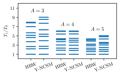
Figure 1: Comparison of the discrete kinetic energy spectra for $A=3,4,5$ hypernuclei in the Y-NCSM and in the corresponding $D=3(A-1)$ dimensional hyper-radial well (HRW). In each case, the spectrum is plotted in units of the smallest eigenvalue.

II.3 Interactions

A main focus of this work is to explore the importance of nuclear physics uncertainties. For this purpose we employ the family of 42 different NNLO_sim interactions Carlsson et al. (2016) that are based on $\chi$EFT for nuclear systems up to next-to-next-to-leading order (NNLO). At this order, which is employed here, the nuclear interaction includes $N\!N$ as well as $N\!N\!N$ forces. The 26 LECs of this interaction are optimized to simultaneously reproduce $N\!N$ as well as $\pi\!N$ scattering cross sections, the binding energies and charge radii of ^2,3H and ³He, the quadrupole moment of ²H and the Gamow-Teller matrix element associated with the beta-decay of ³H . Each NNLO_sim potential is associated with one of seven different regulator cutoffs $\Lambda_{N\!N}=450,475,\ldots,575,600\,\mathrm{MeV}$. In addition, the database of experimental $N\!N$ scattering cross sections used to constrain the respective interaction was also varied. To be precise, it was truncated at six different maximum scattering energies in the laboratory system $T_{\rm Lab}^{\rm max}=125,158,\ldots,257,290\,\mathrm{MeV}$. A detailed description of the NNLO_sim interactions and the optimization protocol is given in Ref. Carlsson et al. (2016) . The 42 different parametrizations of the nuclear interaction at this NNLO order give equally good descriptions of the relevant set of calibration data in the nucleonic sector. Applying all of them within the ab initio description of light hypernuclei will allow us to expose the magnitude of systematic model uncertainties that stems from the truncated EFT description of the nuclear interaction.

For the $Y\!N$ interaction we use the coupled-channel Bonn–Jülich SU(3)-based $\chi$EFT model constructed at LO Polinder et al. (2006). At LO, $V_{Y\!N}$ consists of pseudoscalar $\pi$, $K$ and $\eta$ meson exchanges, together with baryon–baryon contact interaction terms. The meson–baryon coupling constants and the form of the contact interaction is constrained by the SU(3) flavor symmetry. The interaction is regularized in momentum space by a smooth regulator, $f(p^{\prime},p)=\exp(-(p^{4}+p^{\prime 4})/\Lambda_{Y\!N}^{4})$, with momentum cutoff $\Lambda_{Y\!N}$ ranging from 550 to 700 MeV. Unless otherwise specified we are using $\Lambda_{Y\!N}=600\,\mathrm{MeV}$. At LO, there are five free parameters (LECs) which were determined from the fits to the measured low-energy $Y\!N$ scattering cross sections, additionally conditioned by the existence of a bound $\prescript{3}{\Lambda}{\text{H}}$ state with $J^{\pi}=\frac{1}{2}^{+}$ Polinder et al. (2006).

The NNLO_sim $N\!N$ and Bonn–Jülich LO $Y\!N$ interactions are constructed in particle basis, rather than isospin basis. To evaluate the corresponding matrix elements between good-isospin HO states we use the prescription described in Ref. Wirth et al. (2018). This procedure gives excellent agreement with particle-basis calculations, as demonstrated in Ref. Wirth et al. (2018), where the difference between total energies calculated in particle and isospin bases was found to be a few keV for $A=3,4$ hypernuclei. In the following, we neglect this small contribution to the method uncertainty.

III Bayesian approach to infrared extrapolation

III.1 Infrared extrapolation formalism

Having established the IR and UV length scales of the Y-NCSM basis in Sec. II.2 we will employ an IR extrapolation formalism Furnstahl et al. (2012) to extract the infinite-model-space energy eigenvalue, $E_{\infty}$, from results, $E(L_{\mathrm{IR}}{}_{i})$, computed at truncated bases

$$E(L_{\mathrm{IR}})=E_{\infty}+a_{0}\exp{(-2\kappa_{\infty}L_{\mathrm{IR}})},$$ (19)

where $L_{\mathrm{IR}}=L_{\mathrm{IR}}(A,N_{\mathrm{max}},\hbar\omega)$ Wendt et al. (2015). In addition, there will be UV corrections to the computed energies. These errors can be minimized by inferring the extrapolation parameters using computational results obtained at large and fixed $\Lambda_{\mathrm{UV}}$ Forssén et al. (2018). Specifically, we will work at fixed $\Lambda_{\mathrm{UV}}=1200\,\mathrm{MeV}$ which provides a good compromise between the performance of reliable extrapolation and the minimization of UV corrections, as demonstrated in Fig. 2. Note that $\hbar\omega$ can be tuned for fixed $N_{\mathrm{max}}$ to set different UV scales. Here we used Gaussian Process (GP) regression (with an RBF kernel) Rasmussen and Williams (2006) to interpolate in HO frequency for fixed $N_{\mathrm{max}}$. The training data was composed of computed results at even, integer values of $\hbar\omega\in[6,40]$ MeV. With this setup, and using the GPy module GPy (since 2012), we find that the standard deviation for a predicted energy is less than 0.5 keV at any (interpolated) value of $\hbar\omega$.

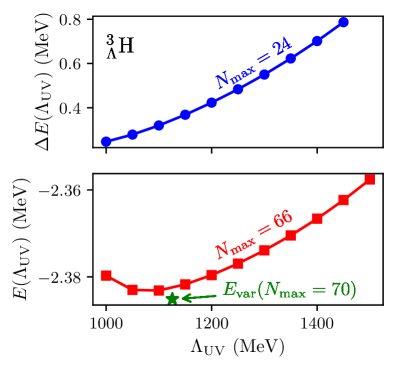
Figure 2: The ground-state energy for $\prescript{3}{\Lambda}{\text{H}}$ at fixed $N_{\mathrm{max}}$ as a function of the UV scale $\Lambda_{\mathrm{UV}}$. The results at fixed $\Lambda_{\mathrm{UV}}$ are obtained using GP interpolation as described in the text. The UV-dependence of the extrapolation distance for smaller model spaces (upper panel) and the region of the variational minimum at very large model spaces (lower panel) indicates the $\Lambda_{\mathrm{UV}}\lesssim 1200\,\mathrm{MeV}$ is a good choice for performing IR-extrapolation.

Subleading IR corrections to Eq. (19), here denoted $\Delta E_{\text{IR},\text{NLO}}$, are proportional to $\exp{(-2\kappa_{\infty}L_{\mathrm{IR}})}/(\kappa_{\infty}L_{\mathrm{IR}})$ as demonstrated in the two-body case Furnstahl et al. (2014). In many-body systems, further corrections from additional separation channels are expected to be of the order of $\exp{(-2k_{\mathrm{sep}}L_{\mathrm{IR}})}$, Forssén et al. (2018), where $k_{\mathrm{sep}}$ is the relevant momentum scale. However, the latter corrections will be suppressed in the present cases since the $\Lambda$-separation threshold is much below other decay channels.

In practice, we will have computational results up to some largest model space that translates into a maximum IR length, $L_{\mathrm{IR,max}}$. We define

$$\Delta L_{\mathrm{IR}}\equiv L_{\mathrm{IR}}-L_{\mathrm{IR,max}},$$ (20)

and replace the extrapolation factor $a_{0}$ that appear in Eq. (19) with a new parameter

$$\Delta E_{\mathrm{IR}}\equiv a_{0}\exp{(-2\kappa_{\infty}L_{\mathrm{IR,max}})}.$$ (21)

This transformed parameter corresponds to the size of the LO IR energy correction for our largest model-space result. Furthermore, we introduce a random variable $\epsilon_{\mathrm{NLO}}$ that is expected to be of natural size and that will provide a stochastic model for the NLO energy correction. Consequently, we have the extrapolation model

$$\begin{split}E(L_{\mathrm{IR}})=E_{\infty}+\Delta E_{\mathrm{IR}}\exp{(-2\kappa_{\infty}\Delta L_{\mathrm{IR}})}\\ \times\left(1+\frac{\epsilon_{\mathrm{NLO}}}{\kappa_{\infty}(L_{\mathrm{IR,max}}+\Delta L_{\mathrm{IR}})}\right).\end{split}$$ (22)

We also note that the $\kappa_{\infty}$ parameter is related to the lowest separation energy threshold of the many-body system Forssén et al. (2018). From the asymptotic form of the wave function

$$\exp{\left(-k_{\mathrm{sep}}r_{\mathrm{sep}}\right)}=\exp{\left(-\kappa_{\infty}\xi_{A-1}\right)},$$ (23)

and assuming that the lowest separation energy is well below the second lowest one, we get that $\kappa_{\infty}$ from the fit should be related to $k_{\mathrm{sep}}$ by

$$\kappa_{\infty}=\sqrt{\frac{m_{N}}{\mu_{A,A-1}}}k_{\mathrm{sep}}=\frac{1}{\hbar}\sqrt{2m_{N}E_{\mathrm{sep}}},$$ (24)

where we have used the relations in Eqs. (17) and (18). In the following we will use $\kappa_{\mathrm{sep}}^{\mathrm{exp}}$ ($\kappa_{\mathrm{sep}}^{\mathrm{th}}$) to denote the momentum associated with the lowest experimental (theoretical) separation threshold energy while $\kappa_{\infty}$ will always be the fit parameter. Higher-order corrections, such as the effects of other separation channels, will in practice lead to $\kappa_{\infty}\gtrsim\kappa_{\mathrm{sep}}^{\mathrm{th}}{}$.

III.2 Bayesian inference

The application of the extrapolation model (22) becomes an inference problem that we tackle using a Bayesian approach. Our Y-NCSM computations for a specific Hamiltonian provide a set of $N$ energies $\mathcal{D}=\{E(L_{\mathrm{IR}}{}_{,1}),E(L_{\mathrm{IR}}{}_{,2}),\ldots,E(L_{\mathrm{IR,max}})\}$ obtained in different model spaces (corresponding to IR cutoffs $L_{\mathrm{IR}}{}_{,1}<L_{\mathrm{IR}}{}_{,2}<\ldots<L_{\mathrm{IR,max}}$). We will assume that the corresponding vector of NLO errors, $\vec{}\epsilon_{\mathrm{NLO}}$, is normally distributed $\operatorname{pr}(\vec{}\epsilon_{\mathrm{NLO}})=\mathcal{N}(0,\Sigma)$. The specification of the covariance matrix $\Sigma$ will involve additional model parameters. With $\vec{\alpha}$ the vector of model parameters (IR extrapolation model plus statistical error model) this assumption implies that the data likelihood $\operatorname{pr}(\mathcal{D}\,|\,\vec{\alpha})$ becomes a normal distribution. As mentioned, the stochastic variable(s) $\epsilon_{\mathrm{NLO}}$ are expected to be of natural size, which we express as $\text{Cov}\left(\epsilon_{\mathrm{NLO}}{}(L_{\mathrm{IR}}{}_{,i}),\epsilon_{\mathrm{NLO}}{}(L_{\mathrm{IR}}{}_{,i})\right)=\bar{\epsilon}{}^{2}$ with $\bar{\epsilon}$ of order unity. Furthermore, we expect that the NLO correction is a rather smooth function of $L_{\mathrm{IR}}$, which we translate into an assumption of positive correlations $0<\text{Cov}\left(\epsilon_{\mathrm{NLO}}{}(L_{\mathrm{IR}}{}_{,i}),\epsilon_{\mathrm{NLO}}{}(L_{\mathrm{IR}}{}_{,i+1})\right)/\bar{\epsilon}{}^{2}<1$. We adopt a rather simple model for this correlation structure that involves a single unknown parameter $\rho$ describing the correlation coefficient between two subsequent model space results. The expected decay of the correlation strength with increasing IR distance is here implemented by assigning a Toeplitz structure to the correlation matrix

$$C=\begin{pmatrix}1&\rho&\rho^{2}&\cdots&\rho^{N-1}\\ \rho&1&\rho&\cdots&\rho^{N-2}\\ \rho^{2}&\rho&1&&\vdots\\ \vdots&\vdots&&\ddots\\ \rho^{N-1}&\rho^{N-2}&\cdots&&1\end{pmatrix}.$$ (25)

We note that the $N\times N$ covariance matrix $\Sigma$ is determined by the two parameters $\bar{\epsilon}$ and $\rho$.

The calibration of all model parameters $\vec{\alpha}=\{E_{\infty},\Delta E_{\mathrm{IR}},\kappa_{\infty},\bar{\epsilon},\rho\}$ is an inference problem that we approach using Bayes formula

$$\operatorname{pr}(\vec{\alpha}\,|\,\mathcal{D})\propto\operatorname{pr}(\mathcal{D}\,|\,\vec{\alpha})\operatorname{pr}(\vec{\alpha}).$$ (26)

The probability density function (PDF) on the left-hand side of Eq. (26) is the posterior which is proportional to the product of the likelihood PDF for the data (conditional on model parameters) and the prior PDF for the parameters. We will usually refer to these PDFs as just posterior, likelihood, and prior, respectively.

The first step is then to formulate our prior beliefs for the model parameters.

III.3 Priors for model parameters

First we note that the original parametrization of the extrapolation formula (19) is characterized by a very strong correlation between model parameters $a_{0}$ and $\kappa_{\infty}$ Forssén et al. (2018). Using the transformed parameters, $\Delta E_{\mathrm{IR}}$ and $\kappa_{\infty}$, we expect to find more independent constraints. In fact, we will make no prior assumption of correlations and will assign full factorization

$$\operatorname{pr}(\vec{\alpha})=\operatorname{pr}(E_{\infty})\operatorname{pr}(\Delta E_{\mathrm{IR}})\operatorname{pr}(\kappa_{\infty})\operatorname{pr}(\bar{\epsilon})\operatorname{pr}(\rho).$$ (27)

Our choices of priors for $E_{\infty}$, $\Delta E_{\mathrm{IR}}$, and $\kappa_{\infty}$ are guided by studies of the $N_{\mathrm{max}}$ and $\hbar\omega$ dependence of our results. At this stage we focus on HO frequencies close to the variational minimum rather than the large values that are used for the IR extrapolation model inference. The key output of this pre-study is $(E_{\mathrm{var}},\Delta E_{\mathrm{IR,max}})$ where $E_{\mathrm{var}}$ is the (approximate) variational minimum and $\Delta E_{\mathrm{IR,max}}$ is a very generous estimate for the maximum extrapolation distance. Furthermore, we use $E_{\mathrm{var}}$ to compute a very rough estimate of the separation energy and the associated momentum scale $\kappa_{\mathrm{sep}}^{\mathrm{th,var}}=\sqrt{2E_{\mathrm{sep}}^{\mathrm{th,var}}m_{N}}/\hbar$. We can now specify conservative prior bounds implemented via uniform distributions

$$\operatorname{pr}(E_{\infty}{}) =\mathcal{U}(E_{\mathrm{var}}-\Delta E_{\mathrm{IR,max}},E_{\mathrm{var}}{}+\delta E_{\mathrm{var}}{}),$$ (28)

$$\operatorname{pr}(\Delta E_{\mathrm{IR}}{}) =\mathcal{U}(0,\Delta E_{\mathrm{IR,max}}),$$ (29)

$$\operatorname{pr}(\kappa_{\infty}{}) =\mathcal{U}(\frac{\kappa_{\mathrm{sep}}^{\mathrm{th,var}}}{3},3\kappa_{\mathrm{sep}}^{\mathrm{th,var}}),$$ (30)

where $\delta E_{\mathrm{var}}=0.1\,\mathrm{MeV}$ is an extra flexibility to allow for possible UV errors at low HO frequencies.

Concerning the error model parameters $\bar{\epsilon}$ and $\rho$ we assign

$$\operatorname{pr}(\rho{}) =\mathcal{U}(0.01,0.99),$$ (31)

$$\operatorname{pr}(\bar{\epsilon}{}) =f(\alpha=1.5,\beta=1.0),$$ (32)

where the former encapsulates our expectation that correlations will be positive but of unknown strength, and the latter is a weakly informative inverse gamma distribution. This particular parametrization gives a main strength for natural values (the probability mass for $\bar{\epsilon}<2.0$ is 0.8) while still allowing for larger values via a significant tail.

III.4 MCMC sampling

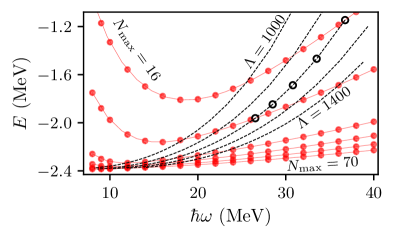
Figure 3: The ground-state energy of $\prescript{3}{\Lambda}{\text{H}}$ as a function of the HO frequency and Y-NCSM model space $N_{\mathrm{max}}$. Results obtained with NNLO_sim($\Lambda_{N\!N}$= 500 MeV, $T_{\rm Lab}^{\rm max}$= 290 MeV) at a subset of fixed $N_{\mathrm{max}}=\{16,24,40,50,60,70\}$ are indicated by filled symbols connected by thin, solid lines. Dashed lines indicate fixed UV scale $\Lambda_{\mathrm{UV}}=\{1000,1100,1200,1300,1400\}$ MeV. The benchmark IR extrapolation shown in Fig. 4 is performed with the GP-interpolated data indicated by open circles.

Having specified the likelihood for the calibration data and the priors for the parameters we are in a position to collect samples from the posterior PDF (26) using Markov Chain Monte Carlo (MCMC) methods. Here we use the affine invariant MCMC ensemble sampler emcee Foreman-Mackey et al. (2013) using up to 100 walkers with 50,000 iterations per walker following 5,000 warmup steps.

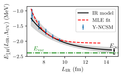
Figure 4: Bayesian IR extrapolation of the ground-state energy for $\prescript{3}{\Lambda}{\text{H}}$ with NLO errors. A truncated data set ($N_{\mathrm{max}}=16-24$) with fixed $\Lambda_{\mathrm{UV}}=1200\,\mathrm{MeV}$ is used for the extrapolation. The posterior IR model prediction is represented by the band that shows the median (black line) and the 68% credible region. The median and 68% credible interval for the $E_{\infty}$ parameter is shown by the black marker with error bar. The green, dashed line indicates the variational minimum obtained at $N_{\mathrm{max}}=70$, $\hbar\omega=9\,\mathrm{MeV}$ Htun et al. (2021). The red line shows a maximum-likelihood fit to the data inversely weighted by the NLO errors.

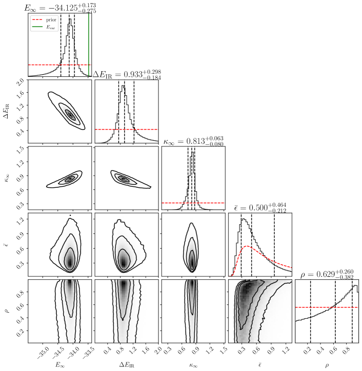
Figure 5: Bayesian extrapolation results for $\prescript{5}{\Lambda}{\text{He}}$ with the NNLO_sim($\Lambda_{N\!N}$= 500 MeV, $T_{\rm Lab}^{\rm max}$= 290 MeV) nuclear interaction, and the Bonn–Jülich LO $Y\!N$ interaction, computed at $N_{\mathrm{max}}=4-10$ and fixed $\Lambda_{\mathrm{UV}}=1200\,\mathrm{MeV}$. Energies are in MeV and $\kappa_{\infty}$ in fm^-1. The median and the 68% equal-tail credible interval are indicated with vertical black, dashed lines for the marginal distributions on the diagonal. The prior distributions are shown by red, dashed lines while the variational estimate for the energy is shown by a green, solid line n the upper left panel. The contour lines for the bivariate distributions indicate 39%, 68%, 86% probability masses.

We check the performance and consistency of our Bayesian approach to IR extrapolation by first studying the $\prescript{3}{\Lambda}{\text{H}}$ system. Here we can perform calculations in very large model spaces up to $N_{\mathrm{max}}=70$ and we have extracted a well-converged variational minimum $E_{\mathrm{var}}=-2.385\,\mathrm{MeV}$ for the NNLO_sim($\Lambda_{N\!N}$= 500 MeV, $T_{\rm Lab}^{\rm max}$= 290 MeV) interaction Htun et al. (2021). For testing purposes, we limit the IR extrapolation data to $N_{\mathrm{max}}\leq 24$. We determine the prior by studying the behavior near the variational minimum, and we select calibration data for the likelihood that has fixed $\Lambda_{\mathrm{UV}}=1200\,\mathrm{MeV}$, see Fig. 3. This implies an extrapolation distance of almost 500 keV as seen in Fig. 4 and we find that a simple maximum likelihood estimation (MLE) fit to the data (with NLO errors as inverse weights) fails to capture the large-$L_{\mathrm{IR}}$ behavior (red, dashed line) and severely underestimates the converged binding energy. In contrast, the Bayesian approach provides extrapolation model samples (gray band) that are consistent with the calibration data. The median (inferred 68% credible interval) for $E_{\infty}$ is $-2.31$ ($[-2.43,-2.26]$) MeV (black symbol with error bar), which encompasses the variational minimum (green, dash-dotted line).

For $\prescript{4}{\Lambda}{\text{H}}$ and $\prescript{4}{\Lambda}{\text{He}}$ $0^{+}$ states we are able to reach $N_{\mathrm{max}}=20$ and the extrapolation distance is less than 100 keV. As will be shown in Sec. IV the extrapolation uncertainty is just $\sim 10\,\mathrm{keV}$. We also compute the $1^{+}$ states in these $A=4$ hypernuclei, but are then limited to $N_{\mathrm{max}}=16$. The extrapolation distance is around 400 keV and, as we will show, the associated uncertainty becomes $\sim 100\,\mathrm{keV}$.

The most challenging calculation is for $\prescript{5}{\Lambda}{\text{He}}$ with computations limited to $N_{\mathrm{max}}\leq 10$ and results not yet close to converged. The variational minimum in this model space is $E_{\mathrm{var}}=-33.48\,\mathrm{MeV}$ while the IR model calibration data extends down to -33.19 MeV. The parameter posterior for the Bayesian extrapolation analysis is shown in Fig. 5. We note the slightly asymmetric mode for $E_{\infty}$, with a long negative tail, and its anti-correlation with $\Delta E_{\mathrm{IR}}$, which is quite expected. The magnitude of the NLO error is smaller than the prior assumption. The correlation coefficient is not that well constrained, but has its main support for rather strong correlations. The bivariate distribution $\operatorname{pr}(\bar{\epsilon},\rho\,|\,\mathcal{D})$ indicates that strongly correlated errors allow for a larger NLO correction which is also expected since the summed penalty in the likelihood decreases with increasing correlation.

The priors and posteriors for all extrapolation parameters for the ground-state energies of $\prescript{4}{\Lambda}{\text{H}}$ and $\prescript{4,5}{\Lambda}{\text{He}}$ and the $1^{+}$ excited states of $\prescript{4}{\Lambda}{\text{H,He}}$ are summarized in Table 3 in the Appendix.

IV Nuclear physics uncertainties

IV.1 Binding and $\Lambda$ separation energies

Energy levels of light hypernuclei are experimentally accessible observables that are sensitive to details of the underlying $Y\!N$ and nuclear interactions. Yet, one can naively expect that calculated $\Lambda$ separation energies—obtained as the differences of the binding energies of hypernuclei and their core nuclei—should be insensitive to the choice of nuclear interaction. In fact, such a rather weak residual dependence of $\Lambda$ separation energies in $A=3,4$ hypernuclei was found already in Faddeev calculations Nogga et al. (2002b) using a limited set of phenomenological $N\!N$ interactions and, more recently, also in NCSM calculations using $\chi$EFT $N\!N$ interaction models Le et al. (2020b). However, our initial analysis for $\prescript{3}{\Lambda}{\text{H}}$ in Ref. Htun et al. (2021) indicated that this dependence may be significantly larger.

In this work we therefore carry a comprehensive systematic study of the variation of the binding and $\Lambda$ separation energies of light hypernuclei resulting from the uncertainties in $N\!N$ and $N\!N\!N$ potentials. In order to quantify this model uncertainty we employed the NNLO_sim family of nuclear interactions Carlsson et al. (2016), specifically designed for such tasks Gazda et al. (2017); Acharya et al. (2016); Htun et al. (2021). In addition, we make use of the Bayesian approach to IR extrapolation from Sec. III to determine the accompanying method uncertainty, associated with the solution of the many-body problem in a truncated Y-NCSM model space.

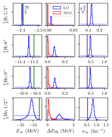
Figure 6: Posterior PDFs for the extrapolated energies (first column) as well as LO and NLO IR corrections (second column) and $\kappa_{\infty}$ (third column) with the NNLO_sim($\Lambda_{N\!N}$= 500 MeV, $T_{\rm Lab}^{\rm max}$= 290 MeV) interaction for $\prescript{3,4}{\Lambda}{\text{H}}$ and $\prescript{4,5}{\Lambda}{\text{He}}$. The variational minimum energies, $E_{\mathrm{var}}$, are shown by green, vertical lines in the first column while the theoretical separation momenta, $\kappa_{\mathrm{sep}}^{\mathrm{th}}$, are shown by purple, vertical lines in the final column. The priors are indicated by dashed, blue lines.

Results of this technique for the ground states of $\prescript{3,4}{\Lambda}{\text{H}}$ and $\prescript{4,5}{\Lambda}{\text{He}}$ are represented in Fig. 6 by posterior PDFs of the extrapolated binding energies (first column) as well as LO and NLO IR corrections (second column) and $\kappa_{\infty}$ (third column) using a single NNLO_sim nuclear interaction with $\Lambda_{N\!N}=500\,\mathrm{MeV}$ and $T_{\rm Lab}^{\rm max}=290\,\mathrm{MeV}$. We note that the precision of the inferred energy, that is represented by the width of the PDF for $E_{\infty}$, depends critically on the extrapolation distance, i.e., the magnitudes of the IR corrections. We also confirm the relation between the $\kappa_{\infty}$ fit parameter and the (theoretical) separation momentum, $\kappa_{\mathrm{sep}}^{\mathrm{th}}$, (here obtained with the median value for $E_{\mathrm{sep}}^{\mathrm{th}}$) as discussed in Sec. III.1.

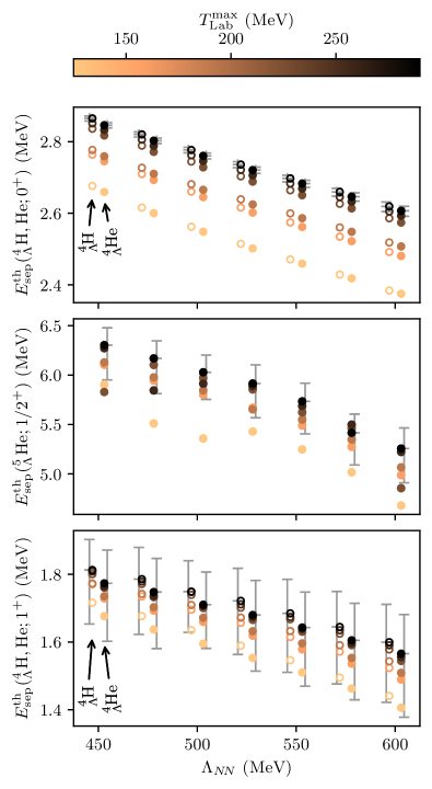
Figure 7: Separation energies for $\prescript{4}{\Lambda}{\text{H}}$ (open circles) and $\prescript{4,5}{\Lambda}{\text{He}}$ (filled circles) ground- and excited states for the family of NNLO_sim interactions. The data corresponds to the medians from the Bayesian IR extrapolation. The 68% credible region from the IR extrapolation is indicated by the error bar for the seven $T_{\rm Lab}^{\rm max}=290\,\mathrm{MeV}$ interactions in the NNLO_sim family.

All inferred parameters of the IR extrapolation are summarized in Table 3 in the Appendix, including also the $1^{+}$ excited states in $\prescript{4}{\Lambda}{\text{H,He}}$ and prior distributions. There, we characterize the posteriors of the parameters by the median value of the distribution plus the 68% and 95% credible intervals. The half width of the 68% credible region, quantifying the extrapolation (method) uncertainty, ranges from 1(10) keV for the ground states of $\prescript{3}{\Lambda}{\text{H}}$ ($\prescript{4}{\Lambda}{\text{H,He}}$), to 100 keV for the excited $1^{+}$ states in $\prescript{4}{\Lambda}{\text{H,He}}$ and 200 keV in $\prescript{5}{\Lambda}{\text{He}}$. These numbers are obtained with the NNLO_sim($\Lambda_{N\!N}$= 500 MeV, $T_{\rm Lab}^{\rm max}$= 290 MeV) interaction. We note (see Fig. 7) that the extrapolation uncertainty becomes larger with increasing $\Lambda_{N\!N}$ regulator cutoff. The main limitation in precision originates in the computation restriction, constraining the feasible size of the Y-NCSM model space truncation $N_{\mathrm{max}}$.

Having assessed the method error, we apply the IR extrapolation for all nuclear interactions in the NNLO_sim family. The $\Lambda$ separation energies for all 42 interactions are shown in Fig. 7 for $\prescript{4}{\Lambda}{\text{H}}$ (open circles) and $\prescript{4,5}{\Lambda}{\text{He}}$ (filled circles) ground- and excited states. The data corresponds to the medians from the Bayesian IR extrapolation while the error bars for the seven $T_{\rm Lab}^{\rm max}=290\,\mathrm{MeV}$ NNLO_sim interactions with different $\Lambda_{N\!N}$ indicate the 68% credible region from the IR extrapolation. We use the variance, $\sigma^{2}\left(\mathrm{NNLO\textsubscript{sim}}\right)$, of predictions for $E_{\mathrm{sep}}^{\mathrm{th}}$ obtained with the full NNLO_sim family to quantify the uncertainty connected to the choice of nuclear Hamiltonian. The resulting model uncertainties

$$\sigma_{\mathrm{model}}\equiv\left[\sigma^{2}\left(\mathrm{NNLO\textsubscript{sim}}\right)\right]^{1/2},$$ (33)

as well as the method uncertainties from the IR extrapolations, are summarized in Table 1 for all hypernuclear states studied in this work. The model uncertainties remain significant despite the fact that the method uncertainties become comparable (or even larger) in magnitude for $\prescript{5}{\Lambda}{\text{He}}$ and the $1^{+}$ excited states of $\prescript{4}{\Lambda}{\text{H,He}}$. It should be noted that each interaction in the NNLO_sim family gives slightly different binding energy for ⁴He Carlsson et al. (2016), which is taken into account when computing the separation energies. For example, the NNLO_sim($\Lambda_{N\!N}$= 500 MeV, $T_{\rm Lab}^{\rm max}$= 290 MeV) interaction gives $E({}^{4}{\text{He}})=-28.10\,\mathrm{MeV}$ . We also note that a direct comparison of $\sigma_{\mathrm{model}}$ with previous studies, such as in Refs. Nogga et al. (2002b); Le et al. (2020b), could be misleading. Usually reported is the total spread of $\Lambda$ separation energies obtained by using a very limited set of nuclear interactions. Moreover, NCSM calculations might additionally suffer from an undesired dependence on the flow parameter of the similarity renormalization group (SRG) transformation applied in order to speed up the convergence. In this work we don’t use SRG transformations but rather make an effort to quantify the method uncertainty associated with the convergence.

Table 1: Separation energies (in MeV) for light hypernuclei. Experimental data is compared with the ab initio result of this work ($E_{\mathrm{sep}}^{\mathrm{th}}$) obtained with NNLO_sim($\Lambda_{N\!N}$= 500 MeV, $T_{\rm Lab}^{\rm max}$= 290 MeV). The 68% credible interval (CI), shown as distances from the median in the next to final column, corresponds to the uncertainty of the extrapolation procedure. The model discrepancy in the final column ($\sigma_{\mathrm{model}}$) is an estimate of the nuclear-interaction uncertainty. The model discrepancy is here quantified by the standard deviation of predictions obtained with the full NNLO_sim family, see Eq. (33).

System	$E_{\mathrm{sep}}^{\mathrm{exp}}$	Ref.	$E_{\mathrm{sep}}^{\mathrm{th}}$
			median	68% CImethod	$\sigma_{\mathrm{model}}$
$\prescript{3}{\Lambda}{\text{H}}$	$0.165(44)\,\mathrm{}$	Eckert et al. (2022)	$0.166\,\mathrm{}$	$[-0.001,+0.001]$	$0.02\,\mathrm{}$
$\prescript{4}{\Lambda}{\text{H}}$	$2.157(77)\,\mathrm{}$	Schulz et al. (2016)	$2.78\,\mathrm{}$	$[-0.01,+0.01]$	$0.08\,\mathrm{}$
$\prescript{4}{\Lambda}{\text{He}}$	$2.39(3)\,\mathrm{}$	Davis (2005)	$2.76\,\mathrm{}$	$[-0.01,+0.01]$	$0.08\,\mathrm{}$
$\prescript{5}{\Lambda}{\text{He}}$	$3.12(2)\,\mathrm{}$	Davis (2005)	$6.03\,\mathrm{}$	$[-0.28,+0.18]$	$0.36\,\mathrm{}$
$\prescript{4}{\Lambda}{\text{H}};1^{+}$	$1.067(80)\,\mathrm{}$	Schulz et al. (2016)	$1.75\,\mathrm{}$	$[-0.12,+0.10]$	$0.07\,\mathrm{}$
$\prescript{4}{\Lambda}{\text{He}};1^{+}$	$0.984(50)\,\mathrm{}$	Yamamoto et al. (2015a)	$1.71\,\mathrm{}$	$[-0.13,+0.10]$	$0.07\,\mathrm{}$

Finally, it should be stressed that all many-body computations discussed so far have been performed with fixed $Y\!N$ regulator cutoff $\Lambda_{Y\!N}=600\,\mathrm{MeV}$. The Bonn–Jülich LO $Y\!N$ interaction is known to result in a noticeable cutoff dependence of separation energies in light $A=3,4$ hypernuclei Nogga (2013b), as well as heavier systems using SRG-evolved $Y\!N$ interactions Wirth et al. (2018); Le et al. (2020b). We find that the $\prescript{5}{\Lambda}{\text{He}}$ binding energy, in particular, is sensitive to the choice of $\Lambda_{Y\!N}$. As shown in Table 2, larger values of $\Lambda_{Y\!N}$ seem to give a better agreement with the experimental separation energy shown in Table 1, but are also associated with a larger extrapolation uncertainty. A more complete study of this sensitivity is left for future work and should possibly also include higher-order descriptions of the $Y\!N$ interaction. We note that most few-body calculations employing various $Y\!N$ interaction models that reproduce ground-state $\Lambda$ separation energies of lighter, $A\leq 4$, hypernuclei yield too large $\prescript{5}{\Lambda}{\text{He}}$ $\Lambda$ separation energy. See Ref. Contessi et al. (2018) for an overview of available calculations and a discussion of this issue within pionless EFT and the implications of the strength of three-body $Y\!N\!N$ interactions for neutron-star matter. The uncertainty quantification presented here should be relevant in the resolution of this puzzle.

Table 2: Separation energies for $\prescript{5}{\Lambda}{\text{He}}$ with different regulator cutoffs for the LO $Y\!N$ interaction. The nuclear interaction ($N\!N$+$N\!N\!N$) is fixed as NNLO_sim($\Lambda_{N\!N}$= 500 MeV, $T_{\rm Lab}^{\rm max}$= 290 MeV). The Bayesian extrapolations are performed at fixed $\Lambda_{\mathrm{UV}}=1200\,\mathrm{MeV}$ including NLO IR errors as described in Sec. III. Median values from the sampled PDFs are shown for the extrapolation distance $\Delta E_{\mathrm{IR}}$ and $E_{\mathrm{sep}}^{\mathrm{th}}$. Furthermore, the 68% and 95% credibility intervals for $E_{\mathrm{sep}}^{\mathrm{th}}$ are shown in the last two columns as distances from the median. All values in MeV.

$\Lambda_{Y\!N}$	$\Delta E_{\mathrm{IR}}$	$E_{\mathrm{sep}}^{\mathrm{th}}$
		median	68% CImethod	95% CImethod
550	$0.72$	$7.33$	[-0.20, +0.13]	[-0.55, +0.30]
600	$0.93$	$6.03$	[-0.28, +0.18]	[-0.75, +0.41]
650	$1.23$	$4.79$	[-0.37, +0.25]	[-0.94, +0.56]
700	$1.56$	$3.82$	[-0.46, +0.33]	[-1.11, +0.69]

IV.2 Charge symmetry breaking

Unlike in nuclei, the amount of CSB in hypernuclei is substantial as it originates in the strong $Y\!N$ interaction. While heavily suppressed in $\prescript{3}{\Lambda}{\text{H}}$ with $T=0$, it manifests itself in the $\Lambda$ separation energy differences of the $A=4$ $\prescript{4}{\Lambda}{\text{H,He}}$ mirror hypernuclei

$$\Delta E_{\mathrm{sep}}^{\mathrm{}}\!\left({\prescript{4}{\Lambda}{\text{H,He}};{J^{\pi}}}\right)\\ =E_{\mathrm{sep}}^{\mathrm{}}\!\left({\prescript{4}{\Lambda}{\text{He}};J^{\pi}}\right)-E_{\mathrm{sep}}^{\mathrm{}}\!\left({\prescript{4}{\Lambda}{\text{H}};J^{\pi}}\right).$$ (34)

The large $\Delta E_{\mathrm{sep}}^{\mathrm{exp}}\!\left({\prescript{4}{\Lambda}{\text{H,He}};{0^{+}}}\right)=0.233(92)\,\mathrm{MeV}$ and negligible $\Delta E_{\mathrm{sep}}^{\mathrm{exp}}\!\left({\prescript{4}{\Lambda}{\text{H,He}};{1^{+}}}\right)=-0.083(94)\,\mathrm{MeV}$ CSB effects in $\prescript{4}{\Lambda}{\text{H,He}}$ ground and excited states, respectively, were reaffirmed recently by precision measurements Nagao et al. (2015); Yamamoto et al. (2015b). These observations provide unique information on the charge dependence of the $Y\!N$ interaction. Given that low-energy $\Lambda p$ cross sections are poorly known and $\Lambda n$ scattering data do not exist, the so far available chiral $Y\!N$ interaction models Polinder et al. (2006); Haidenbauer et al. (2013) have assumed isospin symmetry. Leading CSB terms were only recently incorporated into the chiral NLO $Y\!N$ interaction and constrained to reproduce the measured $\Lambda$ separation energy differences in $\prescript{4}{\Lambda}{\text{H,He}}$ Haidenbauer et al. (2021).

Here we quantify the precision of theoretical predictions for $\Delta E_{\mathrm{sep}}^{\mathrm{th}}\!\left({\prescript{4}{\Lambda}{\text{H,He}};{J^{\pi}}}\right)$, considering both model and method uncertainties. This effort reveals the potential of this observable to constrain the charge dependence of the $Y\!N$ interaction. The sensitivity of the $\Lambda$ separation energy differences on the nuclear interaction model in $0^{+}$ and $1^{+}$ states of $\prescript{4}{\Lambda}{\text{H,He}}$ is shown in Fig. 8, using the charge-symmetric LO $Y\!N$($\Lambda_{Y\!N}$=600 MeV) interaction. The $\Delta E_{\mathrm{sep}}^{\mathrm{th}}\!\left({\prescript{4}{\Lambda}{\text{H,He}};{J^{\pi}}}\right)$ were obtained using the median values of extrapolated $\Lambda$ separation energies, $E_{\mathrm{sep}}^{\mathrm{th}}{(\prescript{4}{\Lambda}{\text{H,He}};{J^{\pi}})}$, for all 42 interactions in the NNLO_sim family. The small residual CSB splittings, $\Delta E_{\mathrm{sep}}^{\mathrm{th}}\!\left({\prescript{4}{\Lambda}{\text{H,He}};{0^{+}}}\right)\approx-0.015\,\mathrm{MeV}$ and $\Delta E_{\mathrm{sep}}^{\mathrm{th}}\!\left({\prescript{4}{\Lambda}{\text{H,He}};{1^{+}}}\right)\approx-0.038\,\mathrm{MeV}$, are due to the increased Coulomb repulsion in $\prescript{4}{\Lambda}{\text{He}}$ compared to its ³He core Bodmer and Usmani (1985) and the $\Sigma N$ intermediate-state mass differences in kinetic energy terms Nogga et al. (2002b); Gal (2015). These results are consistent with previous calculations using different $\chi$EFT nuclear interaction models Gazda and Gal (2016b); Nogga (2019). Since the $\Lambda$ separation energies in $\prescript{4}{\Lambda}{\text{He}}$ and $\prescript{4}{\Lambda}{\text{H}}$ are strongly correlated for each of the NNLO_sim interactions, the model uncertainty, quantified by the variance of their differences, is very small, $\sigma_{\mathrm{model}}\approx 0.002(0.003)\,\mathrm{MeV}$ for the $0^{+}$($1^{+}$) state.

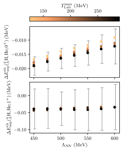
Figure 8: Difference of ground- and excited-state $\Lambda$ separation energies in $\prescript{4}{\Lambda}{\text{He}}$ and $\prescript{4}{\Lambda}{\text{H}}$ for the family of NNLO_sim interactions, calculated using the charge-symmetric LO $Y\!N$($\Lambda_{Y\!N}$=600 MeV) interaction. The data corresponds to the medians from the Bayesian IR extrapolation. The error bars, shown for the seven $T_{\rm Lab}^{\rm max}=290\,\mathrm{MeV}$ interactions in the NNLO_sim family, represent a conservative estimate of the uncertainty obtained from the uncertainties of the separation energies assuming correlated method errors (correlation coefficient $r=0.9$; see text for details).

The uncertainty from the extrapolation procedure, indicated by the error bars in Fig. 8, is larger than the model uncertainty. This is particularly true for the $1^{+}$ states for which our computations are limited to $N_{\mathrm{max}}\leq 16$. Based on a correlation study of $\prescript{4}{\Lambda}{\text{H,He}}$ energies at different $N_{\mathrm{max}}$ we have estimated a correlation coefficient $r=0.9$ between the $\prescript{4}{\Lambda}{\text{H,He}}$ extrapolation errors. This correlation implies that the corresponding error in the difference of the two extrapolated energies becomes a factor $\sqrt{10}$ smaller than with zero correlation (where the total error would be the square root of the quadratic sum). We note that an assignment of uncorrelated errors would in fact have been a much stronger assumption. The resulting method uncertainties are on the order of $\sigma_{\mathrm{method}}\approx 0.005(0.05)\,\mathrm{MeV}$ for the $0^{+}$($1^{+}$) state. In the future, it will be important to perform similar uncertainty quantification studies with $Y\!N$ interaction models incorporating CSB terms.

V Summary and outlook

In this work we have used the ab initio Y-NCSM method to study light hypernuclei up to $\prescript{5}{\Lambda}{\text{He}}$ using realistic chiral interactions as the only simulation input. In particular, we have made a significant effort to quantify relevant nuclear uncertainties which we define as those that are related to the truncation and calibration of the nuclear interaction model plus the error that can be associated with the finite precision of the many-body solver. Quantitative knowledge of these uncertainties is critical for future research efforts in which hypernuclear structure data is used to constrain the elusive $Y\!N$ interaction.

The main findings and conclusions of this study are:

• A comprehensive study of nuclear interaction model uncertainties in hypernuclear observables. We used the NNLO_sim family of 42 realistic nuclear Hamiltonians Carlsson et al. (2016) to study the sensitivity of hypernuclear binding energies to the calibration and regularization of the nuclear interaction. We found that the model uncertainty in the relevant $\Lambda$ separation energies ranges from 20(100) keV in $\prescript{3}{\Lambda}{\text{H}}$ ($\prescript{4}{\Lambda}{\text{H,He}}$) to a few hundred keV in $\prescript{5}{\Lambda}{\text{He}}$.

• Significance of theoretical uncertainty quantification for constraining $\boldsymbol{Y\!N}$ interaction models. We argued that the finite theoretical precision can be quantified and need to be taken into account in future efforts where spectra of light hypernuclei are used to constrain $Y\!N$ interaction models.

• The IR length scale of the truncated Y-NCSM basis was here established using both analytical and numerical arguments. This allowed us to apply rigorous IR corrections to extract model-space converged results.

• Development of a Bayesian IR extrapolation framework. We have developed and used a fully Bayesian framework to perform the IR extrapolation of Y-NCSM results. This allowed the inclusion of both LO and NLO IR corrections in the analysis, introducing various nuisance parameters with prior expectations but conditional on computed data. The method was validated for $\prescript{3}{\Lambda}{\text{H}}$ and used to obtain converged results for light hypernuclei using the full family of NNLO_sim interactions. This (extrapolation) method uncertainty ranges from 1(10) keV for the ground states of $\prescript{3}{\Lambda}{\text{H}}$ ($\prescript{4}{\Lambda}{\text{H,He}}$), to 100 keV for the excited $1^{+}$ states in $\prescript{4}{\Lambda}{\text{H,He}}$ and 200–300 keV in $\prescript{5}{\Lambda}{\text{He}}$ with the main limitation in precision originating in the computation restriction in $N_{\mathrm{max}}$.

• The handling of correlated IR errors. In particular, we presented and applied a simple, stochastic model for the IR corrections that allows to capture correlations between results obtained at different IR length scales. This approach was critical in order to not overestimate the extrapolation errors. Furthermore, it can be straightforwardly applied to other IR extrapolation studies.

• Theoretical precision of CSB energy level splittings in $\boldsymbol{\prescript{4}{\Lambda}{\text{H,He}}}$. We verified that the $\Lambda$ separation energies in $\prescript{4}{\Lambda}{\text{H,He}}$ are strongly correlated and that these correlations considerably reduce the theoretical uncertainties of the CSB energy level splittings. In particular, we showed that the model uncertainty is very small, $\sigma_{\mathrm{model}}\approx 0.002(0.003)\,\mathrm{MeV}$ for the $0^{+}$($1^{+}$) state. This precisely measured observable is therefore sensitive to properties of the $Y\!N$ interaction, such as its poorly known charge dependence.

• Excessive $\boldsymbol{\Lambda}$ separation energy in $\boldsymbol{\prescript{5}{\Lambda}{\text{He}}}$. We have confirmed that the Bonn–Jülich LO $Y\!N$($\Lambda_{Y\!N}$= 600 MeV) yields too large $\Lambda$ separation energy in $\prescript{5}{\Lambda}{\text{He}}$. However, we also found a large sensitivity of this observable to the $\Lambda_{Y\!N}$ cutoff. Larger values of $\Lambda_{Y\!N}$ seem to give a better agreement with the experimental value. Taking into account the considerable theoretical method and model uncertainties, we do not find a strong signal of deficiencies in the Bonn–Jülich LO $Y\!N$ interaction.

*

Appendix A Bayesian inference parameters

See Table 3 for prior and posterior distributions for the parameters used in the Bayesian infrared extrapolations of the ground-state energies of $\prescript{3,4}{\Lambda}{\text{H}}$ and $\prescript{4,5}{\Lambda}{\text{He}}$ and the $1^{+}$ excited states of $\prescript{4}{\Lambda}{\text{H,He}}$.

Table 3: Prior and posterior distributions for the parameters used in the Bayesian infrared extrapolations of the ground state energies of $\prescript{3,4}{\Lambda}{\text{H}}$ and $\prescript{4,5}{\Lambda}{\text{He}}$ and the $1^{+}$ excited states of $\prescript{4}{\Lambda}{\text{H,He}}$. The prior bounds for all parameters (except $\bar{\epsilon}$) are given in the rows labeled “prior”. For $\bar{\epsilon}$ we use a weakly informative inverse gamma distribution for which we present the 95% credible interval. The posteriors are summarized by the median value of the distribution plus the 68% and 95% credible intervals. The theoretical separation momenta, obtained from the medians of the binding energies, are shown in the final column for comparison with $\kappa_{\infty}$ (see Section. III.1).

system			$E_{\infty}$	$\Delta E_{\mathrm{IR}}$	$\bar{\epsilon}$	$\rho$	$\kappa_{\infty}$	$\kappa_{\mathrm{sep}}^{\mathrm{th}}$
$\prescript{3}{\Lambda}{\text{H}}$	prior		[-2.44,-2.29]	[0.00,0.05]	[0.21,9.27]	[0.01,0.99]	[0.03,0.26]
	posterior	median	-2.391	0.007	0.28	0.98	0.13	0.09
		68% CI	[-2.391, -2.390]	[0.006, 0.008]	[ 0.20, 0.36]	[ 0.97, 0.99]	[ 0.12, 0.13]
		95% CI	[-2.392, -2.389]	[0.005, 0.008]	[ 0.15, 0.48]	[ 0.94, 0.99]	[ 0.12, 0.14]
$\prescript{4}{\Lambda}{\text{H}}$	prior		[-11.48,-11.08]	[0.00,0.30]	[0.21,9.27]	[0.01,0.99]	[0.12,1.08]
	posterior	median	-11.26	0.08	0.31	0.93	0.48	0.37
		68% CI	[-11.27, -11.25]	[ 0.07, 0.09]	[ 0.19, 0.52]	[ 0.71, 0.98]	[ 0.46, 0.51]
		95% CI	[-11.29, -11.24]	[ 0.06, 0.11]	[ 0.13, 0.94]	[ 0.24, 0.99]	[ 0.42, 0.54]
$\prescript{4}{\Lambda}{\text{He}}$	prior		[-10.72,-10.32]	[0.00,0.30]	[0.21,9.27]	[0.01,0.99]	[0.12,1.08]
	posterior	median	-10.48	0.08	0.30	0.93	0.48	0.36
		68% CI	[-10.49, -10.47]	[ 0.07, 0.10]	[ 0.19, 0.51]	[ 0.72, 0.98]	[ 0.46, 0.50]
		95% CI	[-10.51, -10.46]	[ 0.06, 0.12]	[ 0.13, 0.93]	[ 0.25, 0.99]	[ 0.42, 0.53]
$\prescript{5}{\Lambda}{\text{He}}$	prior		[-35.48,-33.38]	[0.00,2.00]	[0.21,9.27]	[0.01,0.99]	[0.17,1.53]
	posterior	median	-34.12	0.93	0.50	0.63	0.81	0.54
		68% CI	[-34.40, -33.95]	[ 0.75, 1.23]	[ 0.29, 0.96]	[ 0.25, 0.89]	[ 0.73, 0.88]
		95% CI	[-34.95, -33.73]	[ 0.54, 1.74]	[ 0.18, 2.08]	[ 0.05, 0.97]	[ 0.62, 0.98]
$\prescript{4}{\Lambda}{\text{H}}$;$1^{+}$	prior		[-10.62,-9.77]	[0.00,0.75]	[0.21,9.27]	[0.01,0.99]	[0.09,0.78]
	posterior	median	-10.23	0.36	0.40	0.79	0.48	0.29
		68% CI	[-10.34, -10.14]	[ 0.26, 0.48]	[ 0.23, 0.77]	[ 0.36, 0.96]	[ 0.41, 0.55]
		95% CI	[-10.53, -10.04]	[ 0.18, 0.66]	[ 0.15, 1.62]	[ 0.07, 0.99]	[ 0.32, 0.66]
$\prescript{4}{\Lambda}{\text{He}}$;$1^{+}$	prior		[-9.97,-9.12]	[0.00,0.75]	[0.21,9.27]	[0.01,0.99]	[0.09,0.81]
	posterior	median	-9.43	0.37	0.40	0.78	0.47	0.29
		68% CI	[-9.55, -9.33]	[ 0.28, 0.51]	[ 0.23, 0.76]	[ 0.36, 0.96]	[ 0.40, 0.55]
		95% CI	[-9.76, -9.23]	[ 0.18, 0.68]	[ 0.15, 1.62]	[ 0.07, 0.99]	[ 0.31, 0.66]

References

- Davis (2005) D. H. Davis, “50 years of hypernuclear physics: I. The early experiments,” Nucl. Phys. A 754, 3–13 (2005).
- Hashimoto and Tamura (2006) O. Hashimoto and H. Tamura, “Spectroscopy of hypernuclei,” Prog. Part. Nucl. Phys. 57, 564–653 (2006).
- Gal and Hayano (2008) A. Gal and R.S. Hayano, eds., Special Issue on Recent Advances in Strangeness Nuclear Physics, Vol. 804 (2008).
- Gal et al. (2012) Avraham Gal, Osamu Hashimoto, and Josef Pochodzalla, eds., Progress in strangeness nuclear physics. Proceedings, ECT Workshop on Strange Hadronic Matter, Trento, Italy, September 26-30, 2011, Vol. 881 (2012).
- Gibson et al. (2010) Benjamin F. Gibson, Kenichi Imai, Toshio Motoba, Tomofumi Nagae, and Akira Ohnishi, eds., Proceedings, 10th International Conference on Hypernuclear and strange particle physics (HYP 2009): Tokai, Japan, September 14-18, 2009, Vol. 835 (2010).
- Juliá-Díaz et al. (2013) Bruno Juliá-Díaz, Volodymyr Magas, Eulogio Oset, Assumpta Parreño, Artur Polls, Laura Tolós, Isaac Vidaña, and Àngels Ramos, eds., Proceedings, 11th International Conference on Hypernuclear and Strange Particle Physics (HYP 2012): Barcelona, Spain, October 1-5, 2012, Vol. 914 (2013).
- Tamura (2017) H. Tamura, ed., Proceedings, 12th International Conference on Hypernuclear and Strange Particle Physics (HYP 2015): Sendai, Japan, September 7-12, 2015, Vol. 17 (2017).
- Tang and Schumacher (2019) Liguang Tang and Reinhard Schumacher, eds., Proceedings, 13th International Conference on Hypernuclear and Strange Particle Physics (HYP 2018): Portsmouth Virginia, USA, June 24-29, 2018, Vol. 2130 (2019).
- Gal et al. (1971) A Gal, J.M Soper, and R.H Dalitz, “A shell-model analysis of binding energies for the p-shell hypernuclei. I. Basic formulas and matrix elements for N and NN forces,” Ann. Phys. (NY) 63, 53–126 (1971).
- Gal et al. (1972) A Gal, J.M Soper, and R.H Dalitz, “A shell-model analysis of binding energies for the p-shell hypernuclei II. Numerical Fitting, Interpretation, and Hypernuclear Predictions,” Ann. Phys. (NY) 72, 445–488 (1972).
- Gal et al. (1978) A Gal, J.M Soper, and R.H Dalitz, “A shell-model analysis of binding energies for the p-shell hypernuclei III. Further analysis and predictions,” Ann. Phys. (NY) 113, 79–97 (1978).
- Millener (2008) D. John Millener, “Shell-model interpretation of -ray transitions in p-shell hypernuclei,” Nucl. Phys. A 804, 84–98 (2008).
- Millener (2010) D. John Millener, “Shell-model structure of light hypernuclei,” Nucl. Phys. A 835, 11–18 (2010), arXiv:1011.0367 .
- Millener (2012) D. John Millener, “Shell-model calculations for p-shell hypernuclei,” Nucl. Phys. A 881, 298–309 (2012), arXiv:1206.0198 .
- Motoba et al. (1983) Toshio Motoba, Hiroharu Bandō, and Kiyomi Ikeda, “Light p-Shell -Hypernuclei by the Microscopic Three-Cluster Model,” Prog. Theor. Phys. 70, 189–221 (1983).
- Motoba et al. (1985) Toshio Motoba, Hiroharu Bandō, Kiyomi Ikeda, and Taiichi Yamada, “Chapter III. Production, Structure an Decay of Light p -Shell -Hypernuclei,” Prog. Theor. Phys. Supp. 81, 42–103 (1985).
- Hiyama and Yamada (2009) E. Hiyama and T. Yamada, “Structure of light hypernuclei,” Prog. Part. Nucl. Phys. 63, 339–395 (2009).
- Hiyama (2012) E. Hiyama, “Few-Body Aspects of Hypernuclear Physics,” Few-Body Syst. 53, 189–236 (2012).
- Glendenning et al. (1993) N. K. Glendenning, D. Von-Eiff, M. Haft, H. Lenske, and M. K. Weigel, “Relativistic mean-field calculations of and hypernuclei,” Phys. Rev. C 48, 889–895 (1993).
- Vretenar et al. (1998) D. Vretenar, W. Pöschl, G. A. Lalazissis, and P. Ring, “Relativistic mean-field description of light hypernuclei with large neutron excess,” Phys. Rev. C 57, R1060–R1063 (1998).
- Vidaña et al. (2001) I. Vidaña, A. Polls, A. Ramos, and H.-J. Schulze, “Hypernuclear structure with the new Nijmegen potentials,” Phys. Rev. C 64, 044301 (2001).
- Haidenbauer and Vidana (2020) Johann Haidenbauer and Isaac Vidana, “Structure of single- hypernuclei with chiral hyperon-nucleon potentials,” Eur. Phys. J. A 56, 55 (2020), arXiv:1910.02695 [nucl-th] .
- Lonardoni et al. (2013) Diego Lonardoni, S. Gandolfi, and F. Pederiva, “Effects of the two-body and three-body hyperon-nucleon interactions in hypernuclei,” Phys. Rev. C 87, 041303(R) (2013), arXiv:1301.7472 .
- Lonardoni et al. (2014) Diego Lonardoni, Francesco Pederiva, and Stefano Gandolfi, “Accurate determination of the interaction between hyperons and nucleons from auxiliary field diffusion Monte Carlo calculations,” Phys. Rev. C 89, 014314 (2014), arXiv:1312.3844 .
- Lonardoni et al. (2015) Diego Lonardoni, Alessandro Lovato, Stefano Gandolfi, and Francesco Pederiva, “Hyperon Puzzle: Hints from Quantum Monte Carlo Calculations,” Phys. Rev. Lett. 114, 092301 (2015), arXiv:1407.4448 .
- Wirth et al. (2014) Roland Wirth, Daniel Gazda, Petr Navrátil, Angelo Calci, Joachim Langhammer, and Robert Roth, “Ab Initio Description of p-Shell Hypernuclei,” Phys. Rev. Lett. 113, 192502 (2014), arXiv:1403.3067 .
- Wirth et al. (2018) Roland Wirth, Daniel Gazda, Petr Navrátil, and Robert Roth, “Hypernuclear No-Core Shell Model,” Phys. Rev. C97, 064315 (2018), arXiv:1712.05694 [nucl-th] .
- Le et al. (2020a) Hoai Le, Johann Haidenbauer, Ulf-G. Meißner, and Andreas Nogga, “Implications of an increased -separation energy of the hypertriton,” Phys. Lett. B 801, 135189 (2020a), arXiv:1909.02882 [nucl-th] .
- Le et al. (2020b) Hoai Le, Johann Haidenbauer, Ulf-G. Meißner, and Andreas Nogga, “Jacobi no-core shell model for -shell hypernuclei,” Eur. Phys. J. A 56, 301 (2020b), arXiv:2008.11565 [nucl-th] .
- Miyagawa et al. (1995) K. Miyagawa, H. Kamada, Walter Gloeckle, and V.G.J. Stoks, “Properties of the bound Lambda (Sigma) N N system and hyperon nucleon interactions,” Phys. Rev. C 51, 2905–2913 (1995).
- Nogga et al. (2002a) A. Nogga, H. Kamada, and W. Glöckle, “The Hypernuclei 4He and 4H: Challenges for Modern Hyperon-Nucleon Forces,” Phys. Rev. Lett. 88, 172501 (2002a), arXiv:0112060 [nucl-th] .
- Wirth and Roth (2018) Roland Wirth and Robert Roth, “Light Neutron-Rich Hypernuclei from the Importance-Truncated No-Core Shell Model,” Phys. Lett. B 779, 336–341 (2018), arXiv:1710.04880 [nucl-th] .
- Gazda and Gal (2016a) Daniel Gazda and Avraham Gal, “Ab initio Calculations of Charge Symmetry Breaking in the Hypernuclei,” Phys. Rev. Lett. 116, 122501 (2016a), arXiv:1512.01049 [nucl-th] .
- Gazda and Gal (2016b) Daniel Gazda and Avraham Gal, “Charge symmetry breaking in the A = 4 hypernuclei,” Nucl. Phys. A 954, 161–175 (2016b), arXiv:1604.03434 [nucl-th] .
- Haidenbauer et al. (2021) Johann Haidenbauer, Ulf-G. Meißner, and Andreas Nogga, “Constraints on the -Neutron Interaction from Charge Symmetry Breaking in the - Hypernuclei,” Few Body Syst. 62, 105 (2021), arXiv:2107.01134 [nucl-th] .
- Wirth and Roth (2016) Roland Wirth and Robert Roth, “Induced Hyperon-Nucleon-Nucleon Interactions and the Hyperon Puzzle,” Phys. Rev. Lett. 117, 182501 (2016), arXiv:1605.08677 .
- van Kolck (1994) U. van Kolck, “Few-nucleon forces from chiral lagrangians,” Phys. Rev. C 49, 2932–2941 (1994).
- Epelbaum et al. (2009) E. Epelbaum, H.-W. Hammer, and Ulf-G. Meißner, “Modern theory of nuclear forces,” Rev. Mod. Phys. 81, 1773–1825 (2009).
- Machleidt and Entem (2011) R. Machleidt and D.R. Entem, “Chiral effective field theory and nuclear forces,” Physics Reports 503, 1 – 75 (2011).
- Carlsson et al. (2016) B. D. Carlsson, A. Ekström, C. Forssén, D. Fahlin Strömberg, G. R. Jansen, O. Lilja, M. Lindby, B. A. Mattsson, and K. A. Wendt, “Uncertainty analysis and order-by-order optimization of chiral nuclear interactions,” Phys. Rev. X6, 011019 (2016), arXiv:1506.02466 [nucl-th] .
- Ekström et al. (2015) A. Ekström, G. R. Jansen, K. A. Wendt, G. Hagen, T. Papenbrock, B. D. Carlsson, C. Forssén, M. Hjorth-Jensen, P. Navrátil, and W. Nazarewicz, “Accurate nuclear radii and binding energies from a chiral interaction,” Phys. Rev. C 91, 051301 (2015), arXiv:1502.04682 [nucl-th] .
- Epelbaum et al. (2019) E. Epelbaum et al. (LENPIC), “Few- and many-nucleon systems with semilocal coordinate-space regularized chiral two- and three-body forces,” Phys. Rev. C 99, 024313 (2019), arXiv:1807.02848 [nucl-th] .
- Hüther et al. (2020) Thomas Hüther, Klaus Vobig, Kai Hebeler, Ruprecht Machleidt, and Robert Roth, “Family of Chiral Two- plus Three-Nucleon Interactions for Accurate Nuclear Structure Studies,” Phys. Lett. B 808, 135651 (2020), arXiv:1911.04955 [nucl-th] .
- Jiang et al. (2020) W. G. Jiang, A. Ekström, C. Forssén, G. Hagen, G. R. Jansen, and T. Papenbrock, “Accurate bulk properties of nuclei from to from potentials with isobars,” Phys. Rev. C 102, 054301 (2020), arXiv:2006.16774 [nucl-th] .
- Fujiwara et al. (1996a) Y. Fujiwara, C Nakamoto, and Y Suzuki, “Unified Description of NN and YN Interactions in a Quark Model with Effective Meson-Exchange Potentials,” Phys. Rev. Lett. 76, 2242–2245 (1996a).
- Fujiwara et al. (1996b) Y. Fujiwara, C Nakamoto, and Y Suzuki, “Effective meson-exchange potentials in the SU6 quark model for NN and YN interactions.” Phys. Rev. C 54, 2180–2200 (1996b).
- Rijken et al. (2010) Thomas A. Rijken, M.M. Nagels, and Yasuo Yamamoto, “Baryon-baryon interactions: Nijmegen extended-soft-core models,” Prog. Theor. Phys. Suppl. 185, 14–71 (2010).
- Rijken and Yamamoto (2006) Th.A. Rijken and Y. Yamamoto, “Extended-soft-core baryon-baryon model. II. Hyperon-nucleon interaction,” Phys. Rev. C 73, 044008 (2006), arXiv:nucl-th/0603042 .
- Haidenbauer and Meißner (2005) Johann Haidenbauer and Ulf-G. Meißner, “Jülich hyperon-nucleon model revisited,” Phys. Rev. C 72, 044005 (2005).
- Polinder et al. (2006) Henk Polinder, Johann Haidenbauer, and Ulf-G. Meissner, “Hyperon-nucleon interactions: A Chiral effective field theory approach,” Nucl. Phys. A779, 244–266 (2006), arXiv:nucl-th/0605050 [nucl-th] .
- Haidenbauer et al. (2013) Johann Haidenbauer, S. Petschauer, N. Kaiser, U.-G. Meißner, A. Nogga, and W. Weise, “Hyperon–nucleon interaction at next-to-leading order in chiral effective field theory,” Nucl. Phys. A 915, 24–58 (2013), arXiv:1304.5339 .
- Haidenbauer et al. (2020) J. Haidenbauer, U.-G. Meißner, and A. Nogga, “Hyperon-nucleon interaction within chiral effective field theory revisited,” Eur. Phys. J. A 56, 91 (2020), arXiv:1906.11681 [nucl-th] .
- Baru et al. (2019) V. Baru, E. Epelbaum, J. Gegelia, and X.-L. Ren, “Towards baryon-baryon scattering in manifestly Lorentz-invariant formulation of SU(3) baryon chiral perturbation theory,” Phys. Lett. B 798, 134987 (2019), arXiv:1905.02116 [nucl-th] .
- Ren et al. (2020) X.L. Ren, E. Epelbaum, and J. Gegelia, “Lambda-nucleon scattering in baryon chiral perturbation theory,” Phys. Rev. C 101, 034001 (2020), arXiv:1911.05616 [nucl-th] .
- Bedaque and [van Kolck] (1998) P.F. Bedaque and U. [van Kolck], “Nucleon-deuteron scattering from an effective field theory,” Physics Letters B 428, 221 – 226 (1998).
- [van Kolck] (1999) U. [van Kolck], “Effective field theory of short-range forces,” Nuclear Physics A 645, 273 – 302 (1999).
- Hammer et al. (2020) H. W. Hammer, S. König, and U. van Kolck, “Nuclear effective field theory: status and perspectives,” Rev. Mod. Phys. 92, 025004 (2020), arXiv:1906.12122 [nucl-th] .
- Contessi et al. (2018) L. Contessi, N. Barnea, and A. Gal, “Resolving the Hypernuclear Overbinding Problem in Pionless Effective Field Theory,” Phys. Rev. Lett. 121, 102502 (2018), arXiv:1805.04302 [nucl-th] .
- Beane et al. (2012) S. R. Beane, E. Chang, S. D. Cohen, W. Detmold, H.-W. Lin, T. C. Luu, K. Orginos, A. Parreño, M. J. Savage, and A. Walker-Loud (NPLQCD Collaboration), “Hyperon-nucleon interactions from quantum chromodynamics and the composition of dense nuclear matter,” Phys. Rev. Lett. 109, 172001 (2012).
- Sasaki et al. (2015) Kenji Sasaki, Sinya Aoki, Takumi Doi, Tetsuo Hatsuda, Yoichi Ikeda, Takashi Inoue, Noriyoshi Ishii, and Keiko Murano (HAL QCD), “Coupled-channel approach to strangeness S = 2 baryon–bayron interactions in lattice QCD,” PTEP 2015, 113B01 (2015), arXiv:1504.01717 [hep-lat] .
- Nogga (2013a) A. Nogga, “Light hypernuclei based on chiral and phenomenological interactions,” Nucl. Phys. A 914, 140–150 (2013a).
- Forssén et al. (2018) C. Forssén, B.D. Carlsson, H.T. Johansson, D. Sääf, A. Bansal, G. Hagen, and T. Papenbrock, “Large-scale exact diagonalizations reveal low-momentum scales of nuclei,” Phys. Rev. C 97, 034328 (2018), arXiv:1712.09951 [nucl-th] .
- Navrátil et al. (2009) P. Navrátil, S. Quaglioni, I. Stetcu, and B. R. Barrett, “Recent developments in no-core shell-model calculations,” J. Phys. G36, 083101 (2009), arXiv:0904.0463 [nucl-th] .
- Navrátil et al. (2000) P. Navrátil, G. P. Kamuntavicius, and B. R. Barrett, “Few nucleon systems in translationally invariant harmonic oscillator basis,” Phys. Rev. C61, 044001 (2000), arXiv:nucl-th/9907054 [nucl-th] .
- Stetcu et al. (2007) I. Stetcu, B. R. Barrett, and U. van Kolck, “No-core shell model in an effective-field-theory framework,” Phys. Lett. B 653, 358–362 (2007), arXiv:nucl-th/0609023 .
- Jurgenson et al. (2011) E. D. Jurgenson, P. Navratil, and R. J. Furnstahl, “Evolving Nuclear Many-Body Forces with the Similarity Renormalization Group,” Phys. Rev. C 83, 034301 (2011), arXiv:1011.4085 [nucl-th] .
- Coon et al. (2012) Sidney A. Coon, Matthew I. Avetian, Michael K. G. Kruse, U. van Kolck, Pieter Maris, and James P. Vary, “Convergence properties of \it ab initio calculations of light nuclei in a harmonic oscillator basis,” Phys. Rev. C 86, 054002 (2012), arXiv:1205.3230 [nucl-th] .
- Wendt et al. (2015) K. A. Wendt, C. Forssén, T. Papenbrock, and D. Sääf, “Infrared length scale and extrapolations for the no-core shell model,” Phys. Rev. C 91, 061301(R) (2015), arXiv:1503.07144 .
- König et al. (2014) S. König, S. K. Bogner, R. J. Furnstahl, S. N. More, and T. Papenbrock, “Ultraviolet extrapolations in finite oscillator bases,” Phys. Rev. C 90, 064007 (2014), arXiv:1409.5997 [nucl-th] .
- Note (1) We have corrected the relation between in the one-pion exchange plus contact potential and the LEC multiplying the contact axial-vector current, following the re-derivation by Schiavilla (2018).
- Furnstahl et al. (2012) R. J. Furnstahl, G. Hagen, and T. Papenbrock, “Corrections to nuclear energies and radii in finite oscillator spaces,” Phys. Rev. C 86, 031301 (2012), arXiv:1207.6100 .
- Rasmussen and Williams (2006) C.E. Rasmussen and C.K.I. Williams, Gaussian Processes for Machine Learning, Adaptative computation and machine learning series (University Press Group Limited, 2006).
- GPy (since 2012) GPy, “GPy: A gaussian process framework in python,” http://github.com/SheffieldML/GPy (since 2012).
- Furnstahl et al. (2014) R. J. Furnstahl, S. N. More, and T. Papenbrock, “Systematic expansion for infrared oscillator basis extrapolations,” Phys. Rev. C 89, 044301 (2014), arXiv:1312.6876 .
- Foreman-Mackey et al. (2013) Daniel Foreman-Mackey, David W. Hogg, Dustin Lang, and Jonathan Goodman, “emcee: The mcmc hammer,” Publications of the Astronomical Society of the Pacific 125, 306–312 (2013).
- Htun et al. (2021) Thiri Yadanar Htun, Daniel Gazda, Christian Forssén, and Yupeng Yan, “Systematic Nuclear Uncertainties in the Hypertriton System,” Few Body Syst. 62, 94 (2021), arXiv:2109.09479 [nucl-th] .
- Nogga et al. (2002b) A. Nogga, H. Kamada, and Walter Gloeckle, “The Hypernuclei (Lambda) He-4 and (Lambda) He-4: Challenges for modern hyperon nucleon forces,” Phys. Rev. Lett. 88, 172501 (2002b), arXiv:nucl-th/0112060 .
- Gazda et al. (2017) Daniel Gazda, Riccardo Catena, and Christian Forssén, “Ab initio nuclear response functions for dark matter searches,” Phys. Rev. D 95, 103011 (2017), arXiv:1612.09165 [hep-ph] .
- Acharya et al. (2016) B. Acharya, B. D. Carlsson, A. Ekström, C. Forssén, and L. Platter, “Uncertainty quantification for proton–proton fusion in chiral effective field theory,” Phys. Lett. B 760, 584–589 (2016), arXiv:1603.01593 [nucl-th] .
- Eckert et al. (2022) P. Eckert et al., “Systematic treatment of hypernuclear data and application to the hypertriton,” in 19th International Conference on Hadron Spectroscopy and Structure (2022) arXiv:2201.02368 [physics.data-an] .
- Schulz et al. (2016) F. Schulz et al. (A1), “Ground-state binding energy of H from high-resolution decay-pion spectroscopy,” Nucl. Phys. A 954, 149–160 (2016).
- Yamamoto et al. (2015a) T. O. Yamamoto, M. Agnello, Y. Akazawa, N. Amano, K. Aoki, E. Botta, N. Chiga, H. Ekawa, P. Evtoukhovitch, A. Feliciello, M. Fujita, T. Gogami, S. Hasegawa, S. H. Hayakawa, T. Hayakawa, R. Honda, K. Hosomi, S. H. Hwang, N. Ichige, Y. Ichikawa, M. Ikeda, K. Imai, S. Ishimoto, S. Kanatsuki, M. H. Kim, S. H. Kim, S. Kinbara, T. Koike, J. Y. Lee, S. Marcello, K. Miwa, T. Moon, T. Nagae, S. Nagao, Y. Nakada, M. Nakagawa, Y. Ogura, A. Sakaguchi, H. Sako, Y. Sasaki, S. Sato, T. Shiozaki, K. Shirotori, H. Sugimura, S. Suto, S. Suzuki, T. Takahashi, H. Tamura, K. Tanabe, K. Tanida, Z. Tsamalaidze, M. Ukai, Y. Yamamoto, and S. B. Yang, “Observation of Spin-Dependent Charge Symmetry Breaking in N Interaction: Gamma-Ray Spectroscopy of 4He,” Phys. Rev. Lett. 115, 222501 (2015a), arXiv:1508.00376 .
- Nogga (2013b) A. Nogga, “Light hypernuclei based on chiral and phenomenological interactions,” Nucl. Phys. A 914, 140–150 (2013b).
- Nagao et al. (2015) Sho Nagao et al. (A1 hypernuclear), “Progress of the Hypernuclear Decay Pion Spectroscopy Program at MAMI-C,” JPS Conf. Proc. 8, 021012 (2015).
- Yamamoto et al. (2015b) T. O. Yamamoto et al. (J-PARC E13), “Observation of Spin-Dependent Charge Symmetry Breaking in Interaction: Gamma-Ray Spectroscopy of He,” Phys. Rev. Lett. 115, 222501 (2015b), arXiv:1508.00376 [nucl-ex] .
- Bodmer and Usmani (1985) A. R. Bodmer and Q. N. Usmani, “Coulomb effects and charge symmetry breaking for the hypernuclei,” Phys. Rev. C 31, 1400–1411 (1985).
- Gal (2015) Avraham Gal, “Charge symmetry breaking in hypernuclei revisited,” Phys. Lett. B 744, 352–357 (2015), arXiv:1503.01687 [nucl-th] .
- Nogga (2019) Andreas Nogga, “Charge-symmetry breaking in light hypernuclei based on chiral and similarity renormalization group-evolved interactions,” AIP Conf. Proc. 2130, 030004 (2019).
- Schiavilla (2018) R. Schiavilla, “On the 3N contact potential and 2N contact axial current,” (2018), private communication.