Evaluation and comparison of eight popular Lidar and Visual SLAM algorithms

Abstract

In this paper, we evaluate eight popular and open-source 3D Lidar and visual SLAM (Simultaneous Localization and Mapping) algorithms, namely LOAM, Lego LOAM, LIO SAM, HDL Graph, ORB SLAM3, Basalt VIO, and SVO2. We have devised experiments both indoor and outdoor to investigate the effect of the following items: i) effect of mounting positions of the sensors, ii) effect of terrain type and vibration, iii) effect of motion (variation in linear and angular speed). We compare their performance in terms of relative and absolute pose error. We also provide comparison on their required computational resources. We thoroughly analyse and discuss the results and identify best performing system for the environment cases with our multi-camera and multi-Lidar indoor and outdoor datasets. We hope our findings help one to choose a sensor and the corresponding SLAM algorithm combination suiting their needs, based on their target environment.

I Introduction

Localization and mapping [1] play key roles in various applications, such as, unmanned aerial vehicles [2], unmanned ground vehicles [3], autonomous cars [4], service robots [5], virtual and augmented reality. These technologies are essential components of autonomous robots. They allow a robot to build a map of the environment and to track its relative position within the map. Using the map and the pose information, the robot can perform path planning, navigation, obstacle avoidance, etc.

Nonlinear state estimation methods [1] such as Extended Kalman Filter (EKF) and Unscented Kalman Filter (UKF) using wheel odometry, Inertial Measurement Unit (IMU), and Global Navigation Satellite System (GNSS) are commonly used to estimate the pose of the robot [6]. However, the Kalman filter variants cannot approximate too complex nonlinear functions. Moreover, the GNSS signal is not always available, for example, indoors and among high buildings and dense forrest. Progress in Simultaneous Localization and Mapping (SLAM) [7] holds a promise to perform robust localization and mapping in previously unexplored environments using observations from robot’s onboard sensors such as cameras and Lidars. SLAM methods are suitable for both indoors and outdoors.

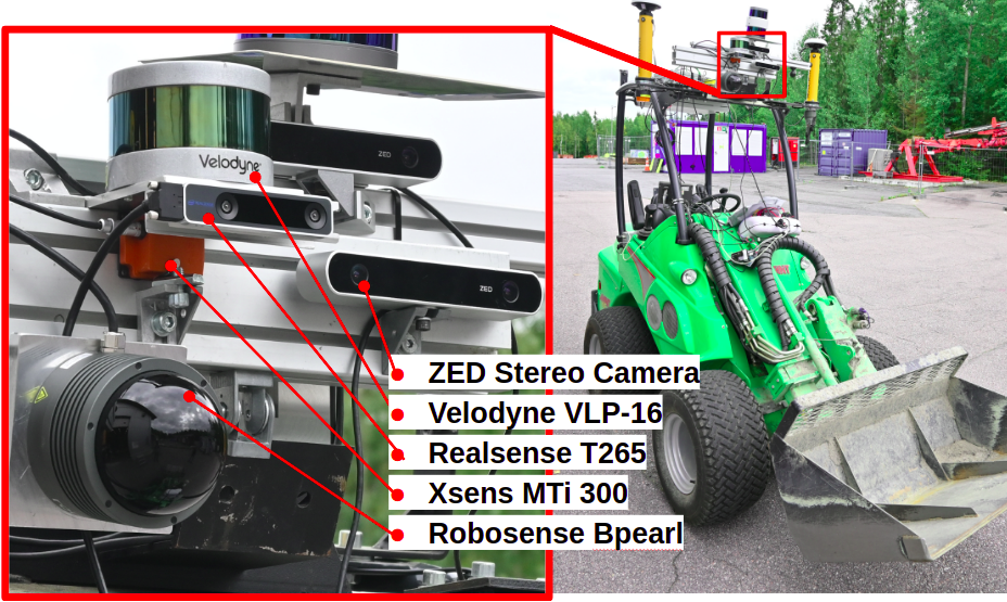
Figure 1: GIM machine used for outdoor data collection with sensor setup mounted on top.

While a number of state-of-the-art SLAM approaches exists [3, 8, 9], to the best of our knowledge there is no systematic comparison. In addition, available public benchmark datasets are either meant for testing visual-inertial SLAM only [10] or do not include different type of sensors [11]. However, different SLAM algorithms utilize different sensor models and types. The goal of this paper is to evaluate and compare the most common state-of-the-art SLAM algorithms using the data from different perception sensors collected simultaneously by robotic set-ups both indoor and outdoor. For a fair comparison of the performance, we used a multi-sensor setup (see Fig 1) including two Lidars, two stereo cameras, a dual antenna GNSS (Global Navigation Satellite System), and a nine-axis inertial measurement unit (IMU) for data collection. The collected data is used to evaluate the 6 degrees of freedom (DoF) localization performance through absolute pose error (APE) and relative pose error (RPE) with respect to the reference ground truth trajectories. We analyze how the design choices made in these SLAM systems affect the accuracy of the trajectory generated by them.

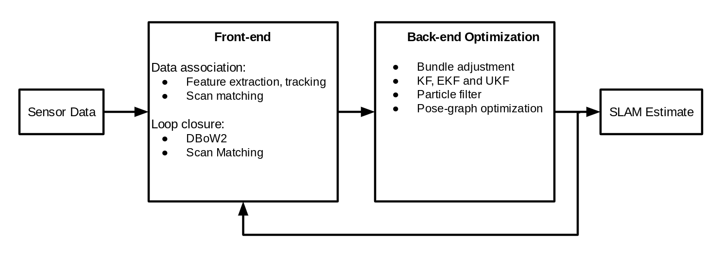
Figure 2: Components of SLAM system (based on [7])

SLAM Benchmarks suites such as Kitti [11] cover urban scenes including highways, rural roads, moving cars, and pedestrians. It has been an essential platform to compare the localization performance of many popular SLAM systems. When selecting a SLAM system for industrial machines, such as autonomous construction machines or other off-road machines, several additional factors have to be considered. These factors include different sensor mounting locations, effects of terrain type, and vibration etc. These effects are not represented in the existing benchmarks. Moreover, to the best of our knowledge, industrial settings are not covered. In this work, we build our set-up to address the effects which have not been covered in the literature. We also build a sensor suite which allows to test both Lidar and visual SLAM methods with data collected simultaneously (with different types of sensors). Some public datasets offer 3D Lidar, stereo camera, and IMU recorded simultaneously (for example, Beach Rover, ETH-challenging, Multi Vech Event [12]), but they are usually recorded without a change of environment and position of sensor mount is not changed. We conduct experiments both indoor and outdoor with varying terrain type. The experiments were conducted during the research for thesis work [13].

Our contributions are as follows. (i) We devise indoor and outdoor experiments to systematically analyse and compare eight popular Lidar and Visual SLAM; (ii) Our experiments are devised to evaluate and compare the performance of the selected SLAM implementations against the mounting position of the sensors, terrain type, vibration effect, and variation in linear and angular speed of the sensors. (iii) We provide comparison on the required computational resources. (iv) We summarize our findings as a collection of recommendations

The paper is organized as follows. In Section II, we explain SLAM, provide some details of the internal working of the selected SLAM algorithms, and introduce the sensor suite. In Section III, we detail the experiment and the environment. In Section IV, we discuss the results. Finally in In Section V we present the conclusions.

II Method

In this section, we describe main components of SLAM algorithms referring to Fig 1, we then explain the SLAM algorithms we have selected to be evaluated referring to Fig 2, and then we explain them into the detail that are relevant to our evaluation purpose.

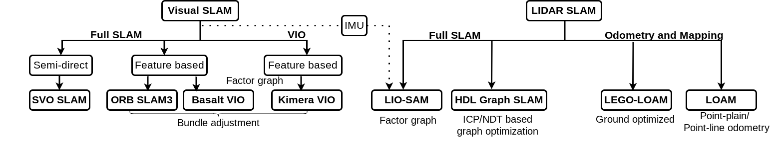
Figure 3: Selected state-of-the-art SLAM algorithms and their tested functionality.

II-A SLAM background

The goal of a 3D SLAM system is to estimate the robot’s 6 DoF pose while simultaneously mapping the new environment using the input sensor data such as images and point clouds. A typical SLAM system consists of two main components: the front-end and the back-end [7] (See Fig. 2).

The front-end processes the incoming visual sensor data extracting useful information from the frames which is then used for robot pose estimation. This step is usually referred to as data association. Visual SLAM front-end receives camera images, extracts key points in each frame [14][15] and tracks them [16] to match the key points between frames. An initial estimate of the robot’s pose can also be generated using methods such as [17]. Key points consistent between the frames are called landmarks. Note that there can be additional constraints in choosing landmarks.

The front-end of Lidar SLAM typically consists of three parts: (i) the point cloud down-sampling to reduce computation, (ii) key point extractions commonly based on the smoothness value of the point cloud voxels [18], and (iii) scan matching such as variants of Iterative Closest Point (ICP) [19] to generate an initial estimate of the pose transform. To reduce the localization error some systems include loop closure by visiting previously visited location. Map is typically represented as either a sparse information on landmark locations or dense point cloud representations in case of Lidar SLAM.

In visual SLAM, the initial pose estimate and the landmark associations from the front-end are utilized in the back-end to perform a maximum-a-posteriori estimate of the robot’s state. In case of Lidar SLAM, the algorithms use odometry from point cloud scan matching instead of landmark associations. Lidar SLAM can also use IMU integration between frames. Recently, with the availability of libraries such as G2O [20] and GTSAM [21], the most popular back-end approach is to use of factor/pose graphs for optimization. It allows users to integrate a wide variety of sensor modalities for more robust state estimation. We present further the details on each of the selected algorithms.

II-B Selection of SLAM algorithms

We picked eight SLAM and odometry algorithms in total, to run our experiments in this paper. They are among the current state-of-the-art and widely used publicly available systems with a version of ROS-based implementations. The algorithms are split into four Lidar-based and four visual algorithms as shown in Fig 3, within them there are both full SLAM and odometry type of algorithms. The essential difference between these is that odometry performs its estimation incrementally frame-by-frame and sometimes performs windowed local optimization, whereas full SLAM approaches aim to maintain global consistency by including loop-closure detection for detecting revisited places for correcting the error in pose estimate. This by design makes Full SLAM approaches computationally heavier than odometry algorithms.

Among the Lidar-based, there are two full SLAM approaches, including LIO SAM [22] and HDL graph SLAM [8] which have loop closure correction, additionally, we used complementary IMU with LIO SAM. The two Lidar odometry algorithms that were used are LEGO LOAM [3] and original LOAM [18] based implementation A-LOAM [23]. We used three full SLAM visual algorithms including SVO2 [24], ORB SLAM3 [9], Basalt VIO [25], and odometry implementation of Kimera VIO [26].

II-C Algorithms Overview

Lidar SLAM: In Lidar based algorithms we included LOAM as it is the building block for many popular Lidar-based SLAM systems including LIO SAM and LEGO LOAM. It is a Lidar odometry algorithm that uses point-to-line and point-to-plane variants of ICP to perform scan match odometry. LEGO LOAM is the other Lidar odometry that we tested, it is very similar to LOAM but achieves efficiency gain by splitting the point cloud into edge and plane features. The algorithm separately extracts height, roll, and pitch from planar features (ground), and X-, Y-coordinates and yaw from edge features.

One of the Lidar-based full SLAM algorithms tested was HDL graph SLAM. It is a factor graph-based approach which allows the user to define multiple edge constraints such as GPS, IMU, floor plane detection, and loop closure. Nodes are added to the graph structure after initial scan matching which is chosen by the user to be either ICP or NDT method. LIO SAM is the second full SLAM Lidar technique we tested. It estimates states utilizing tightly coupled IMU integration and Lidar odometry via factor graph optimization.

Visual SLAM: First in the Vision-based SLAM system is SVO2. Unlike other Visual SLAM algorithms which use keypoint detectors on the front-end, SVO2 has a front-end similar to direct visual SLAM system. There, the estimate is based on sparse model-based image alignment using the local intensity gradient’s direction to estimate the motion. This gives it a faster front-end compared to feature-based systems. Among feature-based SLAM we used ORB SLAM3 which is considered to be one of the current state-of-the-art visual SLAM systems. Its front-end consists of the ORB feature detector and descriptor matching and it offers extra robustness under demanding conditions with its multimap data association DBoW2 posegraph-based loopclosure.

Basalt VIO is the next feature-based visual-inertial algorithm that we used. Basalt recovers the non-linearity in the IMU reading between keyframes which are lost during the more general IMU pre-integration step. The local bundle adjustment estimate generated using FAST features and KLT tracker along with non-linear factors are optimized during global bundle adjustment using factor graphs. Finally, Kimera Visual-inertial odometry from the Kimera C++ library, was developed to perform semantic 3D mesh reconstruction of the environment using metric semantic SLAM. its front-end begins with Shi-Tomasi corners [16] tracked through the new image frames using the KLT tracker. A five-point/three-point RANSAC is then used to solve the relative pose between keyframes, and pre-integrated IMU measurements are calculated between keyframes. The landmarks, initial pose estimate, and IMU pre-integration are used as factor graph constraints to generate the final state estimate.

III Experiments description

In this section, we describe our set-up and the experiments we have conducted to study the effect and severity of following items on accuracy and reliability of the selected SLAM implementations:

• mounting position of the sensors,

• terrain type and vibration effect, and

• variation in linear and angular speed of the sensors.

In outdoor scenarios, we study the effects of all three items, and for indoor case our experiments focuses on (iii).

III-A Experiment set-up

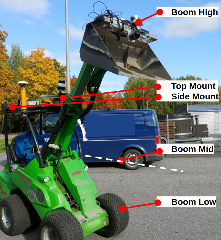
Figure 4: Sensor mounting positions for outdoor experiments.

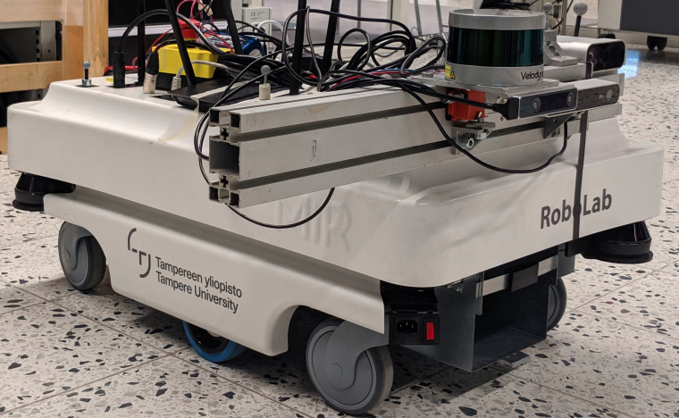
Figure 5: MiR robot used in indoor experiments.

Sensor suite and computation:

In this paper two Lidars, two stereo cameras, and an IMU are used in the sensor setup in Fig 1. Velodyne VLP-16 is a rotating 16 scan Lidar with a vertical field of view of 30 degrees; it offers a vertical resolution of 2 degrees and a horizontal resolution of 0.1 to 0.4 degrees dependent on a rotating speed ranging from 5 to 20 Hz. The second Lidar is the robosense Bpearl; it is likewise a spinning Lidar with a higher 32 scan lines, it has a broader vertical field of view of 90 degrees. With a resolution of 2.81 degrees and a horizontal resolution of 0.2 to 0.4 degrees depending on the speed, which ranges from 10 to 20 Hz. Both Lidars have a maximum range of 100m and a precision of ±3cm. Among the two stereo cameras, Intel Realsense T265 is a global shutter monochrome fisheye camera with a built-in IMU, it has a baseline of 64mm and a field of view of 163 degrees. The second stereo camera is a rolling shutter RGB camera with a larger baseline of 120mm and a vertical and horizontal field of view of 60 and 90 degrees respectively. Finally, the IMU utilized was 9-axis Xsens Mti 300. During the experiments, sensor data was recorded into ROS bag files on a Jetson Xavier NX module with an m.2 SSD running ROS melodic.

In our experiments, Velodyne VLP 16 was used with A-LOAM, LEGO LOAM, HDL graph SLAM, and LIO SAM. We used Realsense T265 with Basalt VIO, SVO2, and Kimera VIO. Kimera VIO did not support the ultra-wide-angle fish-eye model of T265 perfectly and failed in outdoor experiments. Finally, we used the ZED camera with ORB SLAM3. As a result of initial testing, we found these combinations of sensors and algorithms to have the best possible results. We used the same sensor suite in both indoor and outdoor experiments.

The algorithms were running on a 4 core 8 thread Intel i7 7700HQ CPU. In our evaluation, the max capacity of all 8 threads together is considered as 100%. During run-time, the overall usage data is saved into a text file, which is later parsed to separate and calculate the usage corresponding to processes started by the Falgorithms. Outdoor environment: The outdoor tests were conducted at the Mobile Hydraulics Lab of Tampere University. As a ground truth, we used our custom built localization based on dual antenna RTK-GNSS, IMU, and odometry. The sensors were assembled on a frame, and calibrated using Kalibr toolbox [27] for camera-imu calibration and LI-Calib [28] for Lidar-imu calibration . The sensor frame was mounted on top of GIM machine (a multi-purpose wheel loader modified in Tampere University for the purpose of research in autonomous operations- ref MED 09), see Fig 4. Indoor environment: The indoor tests were conducted in RoboLab Tampere of Tampere University. To obtain consistent predefined motion in these trajectories, we mounted the sensor bar on Mobile Industrial Robot (MIR) shown in Fig 5 it is a commercial differential drive mobile robot running Robot Operating System (ROS), generally used to move material within an industrial warehouse space. Through its interface, MIR allows users to define a path that it will execute; this is useful to design and perform repetitive motions for testing SLAM algorithms. Tampere university’s Robolab is equipped with the state-of-the-art Optitrack motion capture system used to collect ground truth. It was used to collect the ground truth trajectory by tracking the markers placed on MIR.

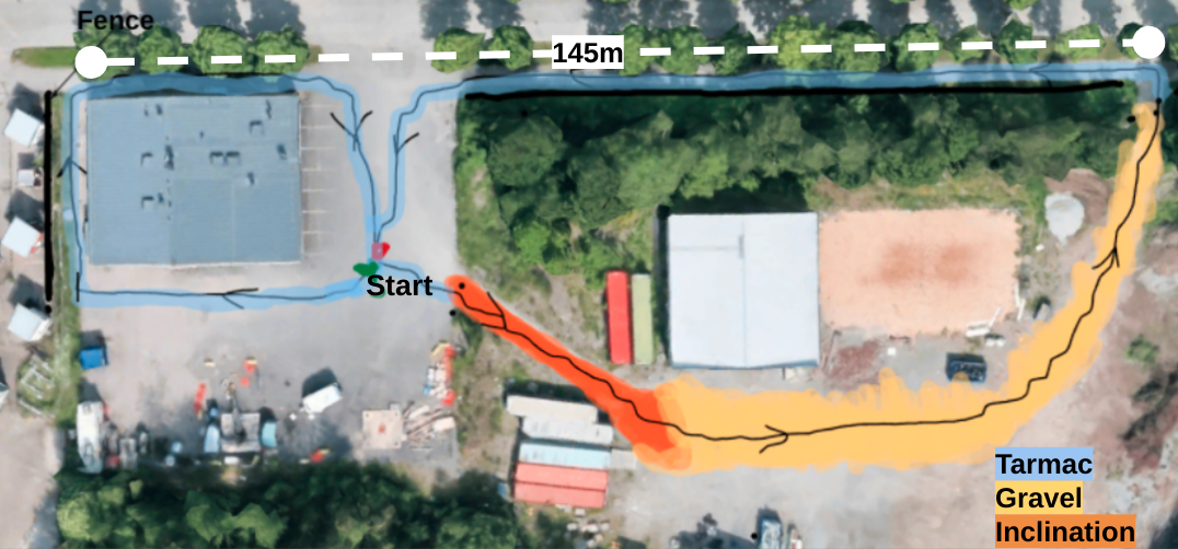
Figure 6: Outdoor experiment 1: top of view of the trajectory to test the effect of various mounting positions and terrain types.

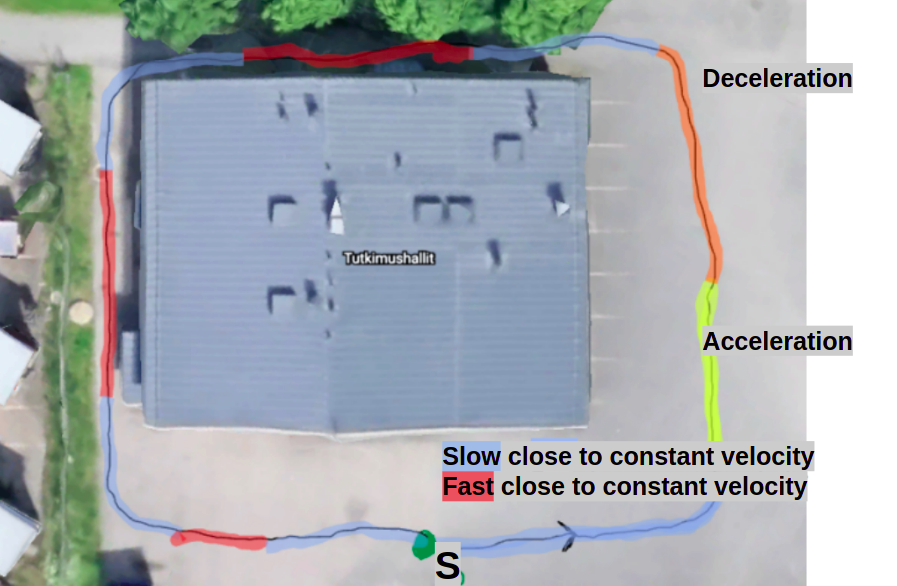
Figure 7: Outdoor experiment 2: top view of of the trajectory to test the effect of variation in linear and angular speed.

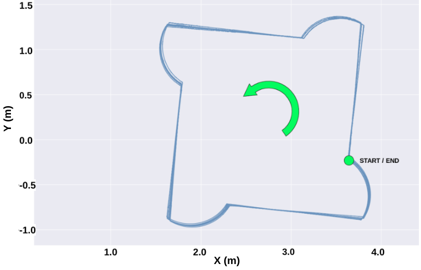
Figure 8: Indoor experiment 1: ground truth sensor trajectory. Notice that the sensor is mounted on the right corner of the MiR robot

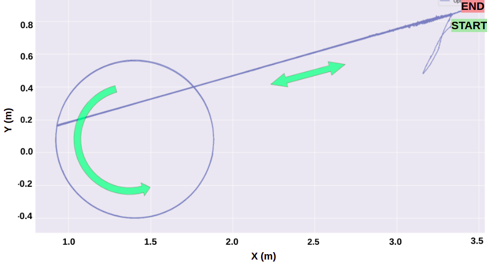
Figure 9: Indoor experiment 2: Optitrack ground truth sensor trajectory.

III-B Outdoor Experiments

Two outdoor experiments were designed to study the effects i-iii mentioned above: one set to study the effect of mounting positions and terrain types, and the second set to study the effect of speed of motion.

Various mounting positions and terrain types (Outdoor experiment 1): These experiments contain five datasets where the machine repeats the same trajectory in the shape of an eight loop around Mobile Hydraulics LAB as shown in Fig  6. In each test, the sensor suite is mounted in different position of the machine (5 positions in total shown in Fig  4): 1) on the boom-low, 2) on the boom-middle, 3) on the boom-high, 4) top mount on the cabin frame, 5) side mount. This experiment allows us to test how the changes in terrain affect the localization performance and benefits of having loop closure after passing through a challenging environment. We also test the sensitivity to vibration effects and sensor mounting position. The trajectory includes straight line on asphalt, straight line on gravel, and downhill path on gravel terrain.

Variation in linear and angular speed (Outdoor experiment 2): In this experiment, we test the rapid changes of machine speed on the localization accuracy of the SLAM algorithms. Sensor motion introduces skew distortion in accumulated point clouds from a Lidar, and motion blur in images where slower feature detectors in the visual SLAM front-end can lose track of the landmarks. This dataset was collected at the same location as the shorter leg of the previous terrain change dataset. The GIM machine starts at the start location S, and it goes around counterclockwise as shown in the Fig 7. During this single loop, the machine goes through changes in velocity such as constant velocity, acceleration, and braking; the loop ends at where it started.

III-C Indoor Experiments

We designed three experiments to study how robust the low-level tracking components are and potential drift in various situations, namely, looping in square, straight line with 360 deg turn, stationary with dynamic scene.

Looping in square (Indoor experiment 1): In the first indoor experiment, MiR was assigned to follow a square-shaped path with two-meter sides in a continuous loop for five minutes as shown in Fig 8, total of  72 meters. This dataset is intended to observe the possible drift in the localization in a constant loop that has panning right-angle turns at each corner of the square, which might have a potential effect on the ability of the feature tracker. Two of the four walls in the Robolab test area are made of glass, with a view of the wider lobby area of the building; this can result in partial reflection of Lidar beams and occlusion due to the objects in front of the glass possibly affecting Lidar SLAM performance.

Mounting position	Boom Low	Boom Mid	Top Mount	Side Mount	Boom High
LOAM	2.062	3.208	1.751	1.669	5.918
LEGO LOAM	1.316	2.759	11.853	8.647	7.891
LIO SAM	2.157	10.778	1.142	1.194	3.467
HDL Graph	1.99	1.474	1.847	3.983	3.337
ORB SLAM3	1.563	3.014	8.641	29.922	13.046
Basalt VIO	2.679	3.360	cam fail	failed	7.094
SVO2	4.559	4.662	cam fail	failed	5.589

TABLE I: Outdoor experiment 1: RMS of Absolute Pose Error (APE) in meters for different mounting positions

Straight line with a 360 turn (Indoor experiment 2): In the second indoor experiment, MiR moves forward on a straight line, starts rotating counterclockwise until it reaches 360 degrees, and returns to the start of the rotation. After this, it returns back in a straight line to the starting point, and repeats the motion with clockwise rotation in the alternative turns, the top view of the trajectory can be seen in Fig 9. The experiment is recorded for five minutes. The 360-degree rotation is meant to induce skew in the point cloud and see how different Lidar SLAMs deal with it. The features are also closer to the sensors as it is indoors resulting in fast moving key-points, rolling shutter distortion and motion blur during the rotation, which could be challenging to slower feature trackers in the visual SLAM algorithms. Additionally, the algorithms would have to re-localize accurately in case of lost features.

Dynamic scene (Indoor experiment 3): The MiR robot is kept stationary throughout the third experiment, but there are moving objects in front of the sensors such as pallets, chairs, and people. The experiment was recorded for five minutes. This dataset allows to measure how dynamic objects affect the accuracy of the SLAM estimate by measuring the drift in the generated pose.

IV Results

Performance metrics: to evaluate the performance, we compute an error between the trajectories generated by the SLAM algorithms and the ground truth. We use Root Mean Square (RMS) of Absolute Pose Error (APE) and Relative Pose Error (RPE), as well as their Standard Deviation (STD).

$$APE_{i}=Q_{i}^{-1}P_{i}$$ (1)

$$RPE_{i+\Delta}=(Q_{i}^{-1}Q_{i+\Delta})^{-1}(P_{i}^{-1}P_{i+\Delta})$$ (2)

$Q_{i}$ is the ground truth transformation between ground truth origin and robot position at time $i$. $P_{i}$ is the estimate of robot in arbitrary SLAM origin. To obtain meaningful APE, we need to align SLAM origin and ground truth’s origin, in this paper, we used least square based Umeyama alignment algorithm [29]. RPE bypasses the alignment problem by comparing the relative poses of the robot between time $i$ and $i+\Delta$ of ground truth and pose estimate.

Outdoor experiments: Table I shows the RMS of APE of the trajectories generated by the SLAM algorithms compared to the ground truth for different sensor mounting positions (Experiment 1 shown in Fig 6).

The ground-optimized LEGO LOAM’s accuracy degrades as the elevation of the sensors increases (i.e., Boom High, Top Mount). LIO SAM, which uses IMU demonstrates the best APE of 1.142m, but its performance degrades when sensors are mounted on the shaky boom. LOAM, which is based on variants of ICP scan matching has the best accuracy in side mount position which provides the largest unobstructed field-of-view of around 270 degrees.

ORB SLAM3 had the least error of 1.563m among all of the visual SLAM algorithms in boom low position. It can also be seen that the accuracy of the overall visual SLAM algorithms goes down as the camera moves away from the ground. In the side mount position, as the camera is perpendicular to the motion of the machine, the key points are moving quickly and the motion blur was high. Data association between frames was rarely possible, resulting in the failure of Basalt VIO and SVO2, but OBR SLAM3 managed to relocalize due to its better data association capabilities although with large error. Realsense T265 hardware failed during the collection of the Top mount dataset, resulting in missing estimates from Basalt VIO and SVO2.

APE	LOAM	LEGO	LIO	HDL	ORB	Basalt	SVO2
		LOAM	SAM	Graph	SLAM3	VIO
RMS	1.072	1.448	3.715	0.845	1.442	1.245	2.919
STD	0.480	0.880	1.701	0.387	0.487	0.452	1.433

TABLE II: Outdoor experiment 2: RMS and STD of Absolute Pose Error (APE) in meters for various speed experiments.

In the second experiment (Fig 7) for varying linear and angular speed, HDL graph SLAM has the least error of 0.845m as shown in Table II, Its loop-closure capability helped in maintaining estimate’s accuracy. The ICP scan match odometry algorithm LOAM performed well with an error of 1.072m, LEGO LOAM has a decent RMS APE of 1.448m as the boom was in boom-mid position with a good view of the ground. LIO SAM performed the worst with an error of 3.715m due to an initialization error. ORB SLAM3 and Basalt VIO had similar errors, both better than the Lidar SLAM algorithms LIO SAM and LeGO LOAM.

	Square loop (Exp. 1)			360 pan (Exp. 2)			Dynamic scene (Exp. 3)
Error	RPE	RPE STD	APE	RPE	RPE STD	APE	Drift from origin	Accumulated distance
LOAM	0.030	0.011	1.505	0.2772	0.0129	0.8316	0.0484	2.4220
LEGO LOAM	0.105	0.108	1.507	0.0972	0.0397	0.8279	0.0058	3.1880
LIO SAM	0.0606	0.037	1.509	0.0551	0.0263	0.8293	0.0165	2.2400
HDL Graph	0.241	0.174	1.449	0.3270	0.2148	0.8392	-	-
ORB SLAM3	0.016	0.008	1.388	0.0232	0.0175	0.8313	0.2345	0.8480
Basalt VIO	0.008	0.003	1.412	0.0084	0.0037	0.8186	0.5398	8.7310
Kimera	0.029	0.012	1.716	0.0342	0.0214	0.8811	0.0016	0.0340
SVO2	0.009	0.003	1.475	0.0086	0.0037	0.8325	0.3648	0.4000

TABLE III: Indoor experiments: RMS, STD of Relative Pose Error (RPE) and APE with respect to the ground truth trajectories. Values are in meters.

Indoor experiments: Results of the first indoor experiment (looping in square) are summarized in Table III. LOAM had the smallest Relative Pose Error (RPE) of 0.030m among the Lidar based algorithms, followed by LIO SAM with an error of 0.0606m among Lidar SLAM algorithms. Visual SLAM algorithms had better RPE than Lidar SLAM, with Basalt having the least error of 0.008m. By comparing the standard deviation, it can be seen that on average Lidar SLAM estimates were noisier compared to visual SLAM estimate The global consistency of the estimates can be interpreted through APE. ORB SLAM3 has the best APE indicating superior loop-closure and global optimization capabilities. Similarly, HDL graph SLAM had the worst RPE results but comparable APE results. It is interesting to note that three Lidar-based algorithms, LOAM, LEGO LOAM, and LIO SAM, have a very close APE of 1.5m. SVO performed better in this dataset than the previous outdoor datasets due to its faster front-end, helping it track features better through the panning 90 degree turns of the square.

Table III shows the RPE and APE from the second indoor experiment in the middle, which has trajectory shown in Fig 9. Visual SLAM algorithms performed better than Lidar SLAM again in RPE, where Basalt has the least RMSE of 0.0084m followed by SVO2 with an error of 0.0086m. ORB SLAM3 has the slower front-end with the ORB detector, compared to the best performing Basalt which uses a less computationally costly FAST detector, ORB SLAM3 constantly lost track of features during the rotation but was able to re-localize to achieve comparable accuracy with its superior loop closure detection and submap merging. LIO-SAM using the IMU pre-integration and IMU point cloud deskewing has the least error among Lidar SLAM with an RPE of 0.0551m.

In the final indoor experiment, the robot is stationary with objects moving in the view, therefore we use the accumulated distance and drift from the starting position as metrics to compare the quality of the SLAM estimate as shown in Table III. The drift from starting point in Lidar-based algorithms is minimal, and they outperformed all vision-based algorithms except Kimera. Pose graph nodes have not been initialized in HDL graph SLAM as the minimum distance necessary has not been exceeded, keeping the estimate at zero. Visual algorithms ORB SLAM3, Basalt VIO, and SVO2 have drifted from the start point around 0.23-0.36m, higher than Lidar SLAM, indicating that smaller field-of-view of the camera compared to Lidar led to greater impact of moving objects. Lidar SLAM estimates were accurate but noisy resulting in the higher accumulated distance although the overall drift was lower.

Usage	Average CPU usage (%)	Peak CPU usage (%)
LOAM	6.637	11.361
LEGO LOAM	4.433	7.880
LIO SAM	21.401	79.650
HDL Graph	11.85	56.120
ORB3	27.743	43.319
Basalt	23.592	59.810
Kimera	38.091	68.327
SVO2	6.463	10.210

TABLE IV: Average and peak CPU usage in % of total available CPU, by the algorithms running the same experiment.

Computational resources: From Table IV we can see that Lidar odometry algorithms LEGO LOAM and LOAM required the least CPU resources with 4.43% and 6.63% respectively due to their simpler algorithms. The CPU utilization of posegraph-based methods LIO SAM and HDL graph SLAM utilizing GTSAM and g2o is 21.4% and 11.85%, respectively, LIO SAM’s higher load reaching almost 80% at peak can be explained by the additional IMU integration that it performs. The impact of feature detectors in the front-end can be observed from their higher average CPU usage compared to the rest in ORB SLAM3, Basalt VIO, and Kimera VIO.

Among all the outdoor experiments, LIO SAM with top mount Lidar position was the most suitable for loader type machines used in our experiments, it had the least RMS of APE of 1.142m. Stability was more important to the IMU dependent LIO SAM whose performance degraded when the sensor was fixed to the loader bucket on the boom which has high vibrations while moving. LeGO LOAM was the most efficient while also having relatively good performance when the sensor is closer to the ground with an APE of 1.316m. With arbitrary LIDAR location, the simpler LOAM had reasonable results, hence making it a suitable choice when the sensor location is not fixed. Visual algorithms performed better when the camera was closer to the ground.

V CONCLUSION

In this paper, we presented systematic evaluation of eight most popular state-of-the-art visual and Lidar SLAM methods. We tested them using our specially designed sensor suite which included visual sensors of different types, allowing us to capture the data from them simultaneously. The experiments were performed both outdoor and indoor, where we studied effects of sensor mounting position, terrain type, vibration effects, and variations in linear and angular velocities.

Among the Lidar SLAM methods, LIO SLAM, using additionally IMU information, produces the smallest error in a single run. LEGO LOAM is suitable for lightweight applications but with sensor mounted closer to the ground. LOAM can used also in lightweight applications with less complex environments. Comparing visual SLAM methods, ORB SLAM 3 performed well in dynamic and difficult environments. Basalt VIO deals better with quick changes in velocities. Thanks to the faster performing front-end, SVO could deal better with fast motion. Overall, Lidar’s consistently were better with outdoor and with dynamic objects due to their large field of view of the environment.

References

- [1] T.. Barfoot “State Estimation for Robotics” Cambridge University Press, 2017
- [2] Patrik Schmuck and Margarita Chli “Multi-uav collaborative monocular slam” In 2017 IEEE International Conference on Robotics and Automation (ICRA), 2017, pp. 3863–3870 IEEE
- [3] Tixiao Shan and Brendan Englot “LeGO-LOAM: Lightweight and Ground-Optimized Lidar Odometry and Mapping on Variable Terrain” In 2018 IEEE/RSJ International Conference on Intelligent Robots and Systems (IROS), 2018, pp. 4758–4765 DOI: 10.1109/IROS.2018.8594299
- [4] Shinpei Kato, Shota Tokunaga, Yuya Maruyama, Seiya Maeda, Manato Hirabayashi, Yuki Kitsukawa, Abraham Monrroy, Tomohito Ando, Yusuke Fujii and Takuya Azumi “Autoware on board: Enabling autonomous vehicles with embedded systems” In 2018 ACM/IEEE 9th International Conference on Cyber-Physical Systems (ICCPS), 2018, pp. 287–296 IEEE
- [5] Tae-jae Lee, Chul-hong Kim and Dong-il Dan Cho “A monocular vision sensor-based efficient SLAM method for indoor service robots” In IEEE Transactions on Industrial Electronics 66.1 IEEE, 2018, pp. 318–328
- [6] “ROS robot localization”, http://docs.ros.org/en/melodic/api/robot_localization/html/index.html
- [7] Cesar Cadena, Luca Carlone, Henry Carrillo, Yasir Latif, Davide Scaramuzza, José Neira, Ian Reid and John J Leonard “Past, present, and future of simultaneous localization and mapping: Toward the robust-perception age” In IEEE Transactions on robotics 32.6 IEEE, 2016, pp. 1309–1332
- [8] Kenji Koide, Jun Miura and Emanuele Menegatti “A portable three-dimensional LIDAR-based system for long-term and wide-area people behavior measurement” In International Journal of Advanced Robotic Systems 16, 2019 DOI: 10.1177/1729881419841532
- [9] Carlos Campos, Richard Elvira, Juan J. Rodríguez, José M. M. and Juan D. “ORB-SLAM3: An Accurate Open-Source Library for Visual, Visual–Inertial, and Multimap SLAM” In IEEE Transactions on Robotics, 2021, pp. 1–17 DOI: 10.1109/TRO.2021.3075644
- [10] D. Schubert, T. Goll, N. Demmel, V. Usenko, J. Stueckler and D. Cremers “The TUM VI Benchmark for Evaluating Visual-Inertial Odometry” In International Conference on Intelligent Robots and Systems (IROS), 2018
- [11] Andreas Geiger, Philip Lenz, Christoph Stiller and Raquel Urtasun “Vision meets Robotics: The KITTI Dataset” In International Journal of Robotics Research (IJRR), 2013
- [12] Younggun Cho “Awesome SLAM Datasets”, https://github.com/youngguncho/awesome-slam-datasets
- [13] C.. Garigipati “Evaluation of Simultaneous Localization and Mapping (SLAM) Algorithms”, 2021
- [14] Ethan Rublee, Vincent Rabaud, Kurt Konolige and Gary Bradski “ORB: An efficient alternative to SIFT or SURF” In 2011 International conference on computer vision, 2011, pp. 2564–2571 Ieee
- [15] Edward Rosten, Reid Porter and Tom Drummond “Faster and better: A machine learning approach to corner detection” In IEEE transactions on pattern analysis and machine intelligence 32.1 IEEE, 2008, pp. 105–119
- [16] Carlo Tomasi and Takeo Kanade “Detection and tracking of point” In Int J Comput Vis 9, 1991, pp. 137–154
- [17] David Nistér “An efficient solution to the five-point relative pose problem” In IEEE transactions on pattern analysis and machine intelligence 26.6 IEEE, 2004, pp. 756–770
- [18] Ji Zhang and Sanjiv Singh “LOAM: Lidar Odometry and Mapping in Real-time.” In Robotics: Science and Systems 2.9, 2014
- [19] S. Rusinkiewicz and M. Levoy “Efficient variants of the ICP algorithm” In Proceedings Third International Conference on 3-D Digital Imaging and Modeling, 2001, pp. 145–152 DOI: 10.1109/IM.2001.924423
- [20] Rainer Kümmerle, Giorgio Grisetti, Hauke Strasdat, Kurt Konolige and Wolfram Burgard “G2o: A general framework for graph optimization” In 2011 IEEE International Conference on Robotics and Automation, 2011, pp. 3607–3613 DOI: 10.1109/ICRA.2011.5979949
- [21] Michael Kaess “GTSAM Library” In GTSAM Library, 2011-2015, https://collab.cc.gatech.edu/borg, 2015
- [22] Tixiao Shan, Brendan Englot, Drew Meyers, Wei Wang, Carlo Ratti and Daniela Rus “LIO-SAM: Tightly-coupled Lidar Inertial Odometry via Smoothing and Mapping” In 2020 IEEE/RSJ International Conference on Intelligent Robots and Systems (IROS), 2020, pp. 5135–5142 DOI: 10.1109/IROS45743.2020.9341176
- [23] “A-LOAM”, https://github.com/HKUST-Aerial-Robotics/A-LOAM
- [24] Christian Forster, Zichao Zhang, Michael Gassner, Manuel Werlberger and Davide Scaramuzza “SVO: Semidirect Visual Odometry for Monocular and Multicamera Systems” In IEEE Trans. Robot. 33.2, 2017, pp. 249–265 DOI: 10.1109/TRO.2016.2623335
- [25] Vladyslav Usenko, Nikolaus Demmel, David Schubert, Jörg Stückler and Daniel Cremers “Visual-inertial mapping with non-linear factor recovery” In IEEE Robotics and Automation Letters 5.2 IEEE, 2019, pp. 422–429
- [26] Antoni Rosinol, Marcus Abate, Yun Chang and Luca Carlone “Kimera: an Open-Source Library for Real-Time Metric-Semantic Localization and Mapping” In 2020 IEEE International Conference on Robotics and Automation (ICRA), 2020, pp. 1689–1696 DOI: 10.1109/ICRA40945.2020.9196885
- [27] Joern Rehder, Janosch Nikolic, Thomas Schneider, Timo Hinzmann and Roland Siegwart “Extending kalibr: Calibrating the extrinsics of multiple IMUs and of individual axes” In 2016 IEEE International Conference on Robotics and Automation (ICRA), 2016, pp. 4304–4311 IEEE
- [28] Jiajun Lv, Jinhong Xu, Kewei Hu, Yong Liu and Xingxing Zuo “Targetless calibration of lidar-imu system based on continuous-time batch estimation” In 2020 IEEE/RSJ International Conference on Intelligent Robots and Systems (IROS), 2020, pp. 9968–9975 IEEE
- [29] S. Umeyama “Least-squares estimation of transformation parameters between two point patterns” In IEEE Transactions on Pattern Analysis and Machine Intelligence 13.4, 1991, pp. 376–380 DOI: 10.1109/34.88573