Instanton effects on electromagnetic transitions of charmonia

Abstract

We investigate the mass spectrum and electromagnetic transitions of charmonia, emphasizing the instanton effects on them. The heavy-quark potential consists of the Coulomb-like potential from one-gluon exchange and the linear confining potential. We introduce the nonperturbative heavy-quark potential derived from the instanton vacuum. We also consider the screened confining potential, which better describes the electromagnetic decays of higher excited states. Using this improved heavy-quark potential, we compute the mass spectrum and electromagnetic decays of the charmonia. Focusing on the instanton effects, we discuss the results compared with the experimental data and those from other works. The instanton effects are marginal on the electromagnetic decays of charmonia.

I Introduction

The quarkonium is the simplest and yet crucial system that consists of one heavy quark and one heavy antiquark among all hadrons. Since it is very heavy, a nonrelativistic (NR) approach is suitable for describing its structure and properties. Moreover, the accurate measurements of masses and radiative decay widths for the low-lying quarkonia provide a precision test of any theory based on perturbative and non-perturbative quantum chromodynamics (see reviews on quarkonia [1, 2, 3, 4]). The quarkonia have successfully been described by quantum mechanical potential models [5, 6]. The static heavy-quark potential consists of two main contributions: The Coulomb-like term and the phenomenological quark-confining one. The former arises from one-gluon exchange (OGE) between a heavy quark ($Q$) and a heavy antiquark ($\overline{Q}$), based on perturbative quantum chromodynamics (pQCD) [7, 8, 9, 10]. Higher-order corrections from pQCD were also considered [11, 12, 13, 14, 15]. Since OGE comes from pQCD, the Coulomb-like potential governs the short-range dynamics inside charmonia. It should fade away as the distance between heavy and anti-heavy quarks and then will be taken over by the effects of the quark confinement [16]. The heavy-quark potential for the quark confinement can be derived phenomenologically from the Wilson loop, which increases monotonically as the distance between heavy quarks increases [5, 6].

While the Coulomb-like and quark-confining terms constitute the main contributions to the static heavy-quark potential, there is still a nonperturbative effect that arises from the instanton vacuum. The nonperturbative heavy-quark potential was derived from the instanton vacuum [17] and was examined by computing the charmonium spectra [18, 19]. While the instanton effects on the heavy-quark potential are small, they provide significant physical implications. Firstly, the heavy quark acquires an additional dynamical mass from the instantons, i.e. $\Delta M_{I}\simeq 70$ MeV [17, 18, 19, 20], which allows one to use the value of the heavy-quark mass close to the physical one in the heavy-quark potential. Secondly, an additional contribution from the instantons makes it possible to employ the value of the strong coupling constant near the charm-quark mass scale. Note that often the strong coupling constant used in the Coulomb-like potential was overestimated [22, 21, 23]. In addition to the instanton effects, we want to modify the linear confining potential. When the $1/m_{Q}$ corrections are considered where $m_{Q}$ is the heavy-quark mass, the heavy quark is no more static. The light quark-antiquark pair will create from the vacuum at a certain scale ($\sim 1$ fm). Furthermore, the created quark-antiquark pair will screen the color charge [24, 25]. The screened confining potential has been adopted to describe the electromagnetic (EM) decays of charmonia [26, 23]. While the EM transitions of the charmonia have extensively been studied within various theoretical frameworks such as the heavy-quark potential models [27, 21, 23], lattice QCD [26, 28, 29, 30, 31, 32, 33], QCD sum rules [34, 35, 36], Bethe-Salpeter equations [37, 38], potential NR QCD (pNRQCD) [39, 40], and quark models [41, 42, 43, 44, 45], the EM decays of higher excited charmonium states are not fully understood theoretically.

In the present work, we want to extend the previous works and examine the instanton effects on the charmonium spectrum and EM transitions of the charmonia. We sketch the current work as follows: In Section II, we briefly explain how the heavy-quark potential is derived from the instanton vacuum. In Section III, we reproduce the mass spectrum of the charmonia with a new type of the confining potential introduced. In Section IV, we derive the spin-dependent part of the heavy-quark potential. In Section V, we discuss the results for the charmonium spectrum and EM decay rates. The final Section is devoted to the summary and conclusion.

II Heavy-quark potential from the instanton vacuum

We begin by recapitulating the derivation of the nonperturbative heavy-quark potential from the instanton vacuum.

II.1 Non-perturbative heavy-quark potential

The heavy-quark potential can be defined by the Wilson loop as shown in Fig. 1.

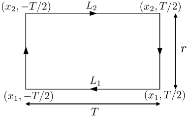
Figure 1: The rectangular Wilson loop along a contour $T\times r$ with $T\rightarrow\infty$. In this limit, one can ignore the spatial line because $r$ is very small compared to $T$.

Diakonov et al. [17] derived the central part of the nonperturbative heavy-quark potential, regarding an instanton packing parameter $\lambda=\bar{\rho}^{4}/R^{4}(\sim 0.01)$ as an expansion parameter, where $\bar{\rho}$ denotes the average instanton size and $R$ the instanton inter-distance that is represented as $R=N/V$. In the instanton liquid model, the number of instanton $N$ and the four dimensional volume $V$ give $N/V\simeq(200\,\rm MeV)^{4}$ and $\bar{\rho}\simeq(600\,\mathrm{MeV})^{-1}\simeq 1/3\,\mathrm{fm}$ [46, 47, 48]. The gluon field $\mathcal{A}_{\mu}(x)$ in Euclidean space can be decomposed into the classical($A$) and quantum($B$) parts

$$\mathcal{A}_{\mu}(x)=A_{\mu}(x,\xi)+B_{\mu}(x),$$ (1)

where the classical background field $A_{\mu}(x,\xi)$ is given by the summation over all (anti)instanton fields $A_{\mu}(x,\xi)=\sum_{i}A_{i\mu}(x,\xi_{i})$. Here, $\xi_{i}=(z_{i},U_{i},\rho_{i})$ denote collective coordinates: the instanton positions $z_{i}$, the color orientations $U_{i}$, and the sizes of the instantons $\rho_{i}$. In the large $N_{c}$ (number of color) limit, the width of the instanton distribution is of order $1/N_{c}$, so the instanton distributions can be approximated by the delta functions. Thus, $\rho_{i}$ is just the average size of the instanton $\bar{\rho}$, $\rho_{i}=\bar{\rho}$. The instanton field $A_{\pm,\mu}$ in the singular gauge is expressed as

$$A_{\pm,\mu}(x,z_{\pm})=\frac{\eta^{\mp}_{\mu\nu}(x-z_{\pm})_{\mu}\lambda^{a}\bar{\rho}^{2}}{(x-z_{\pm})^{2}((x-z_{\pm})^{2}+\bar{\rho}^{2})},$$ (2)

where $\eta_{\mu\nu}^{\mp}$ stand for the ’t Hooft symbols.

$$\eta_{a\mu\nu}^{\pm}=\left\{\begin{array}[]{cc}\epsilon_{a\mu\nu}&:\ \mu,\nu=1,2,3\\ \mp\delta_{a\nu}&:\ \mu=4\\ \pm\delta_{a\mu}&:\ \nu=4\\ 0&:\ \mu,\nu=4\end{array}\right.$$ (7)

Here, the $+$ and $-$ signs designate respectively the instanton and the antiinstanton. Note that the heavy-quark and antiquark correlator is just the same as the Wilson loop [49]. Considering that the instanton medium is dilute, we can average over the pesudoparticles (instantons and antiinstantons) independently. Thus, the average of the Wilson loop over the pseudoparticles can be expressed as

$$w\equiv\langle\kern-2.4pt\langle W\rangle\kern-2.4pt\rangle =\int d\xi\frac{1}{D^{(1)}}\frac{1}{D^{(2)}},$$ (8)

where $d\xi=V^{-1}\prod_{i=1}dz_{i}dU_{i}$ stands for the measure of the zero modes and $D^{(i)}$ is the inverse of the heavy-quark propagator expressed by $D^{(i)}=\theta^{-1}-\sum_{I}a_{I}^{(i)}$. The double angle brackets represent the ensemble average over the pesudoparticles [17]. $\theta$ designates the inverse of the time derivative $d/dt$: $\langle t|\theta|t^{\prime}\rangle=\theta(t-t^{\prime})$ with the Heaviside step function $\theta(t-t^{\prime})$. $a_{I}^{(i)}$ represent $a_{I}^{(i)}=iA_{I,\mu}^{(i)}(\xi)\dot{x}_{\mu}(t)$, which is aligned along the tangential direction to the Wilson line. The superscripts in Eq. (8) denote the corresponding Wilson lines as shown in Fig. 1. After the integral over the color-orientations and using the Pobylitsa equation [50], we obtain the inverse of the Wilson loop in powers of $N/VN_{c}$

$$w^{-1}=\theta^{-1}\theta^{-1}+\frac{N}{2VN_{c}}\mathrm{Tr}_{c}\sum_{\pm}\int d^{4}z_{\pm}$$ (9)

$$\times\left[\theta^{-1}\theta^{-1}-\theta^{-1}w_{\pm}^{(1)}\theta^{-1}\theta^{-1}w_{\pm}^{(2)}\theta^{-1}\right]$$ (10)

$$+\mathcal{O}\left(\left(\frac{N}{2VN_{c}}\right)^{2}\right),$$ (11)

where $\mathrm{Tr}_{c}$ is the trace over color space. $w_{\pm}$ is defined as

$$w_{\pm}=(\theta^{-1}-a_{\pm})^{-1}.$$ (12)

Performing the Fourier transformation [17], we obtain

$$\langle t_{1}^{(1)}|w|t_{1}^{(2)}\rangle=\int\frac{d\omega}{2\pi}e^{i\omega(t_{1}^{(1)}-t_{1}^{(2)})}\frac{1}{w^{-1}(\omega)},$$ (13)

where $t_{1}^{(1)}$ and $t_{1}^{(2)}$ are $-T/2$ in $L_{1}$ and $-T/2$ in $L_{2}$, respectively. In the infinite time limit $T\rightarrow\infty$, the heavy quark potential is defined by the Wilson loop as follows

$$\langle t_{1}^{(1)}|w|t_{1}^{(2)}\rangle \approx\exp\left[-V_{I}T\right],$$ (14)

where $V_{I}$ denotes the instanton-induced potential, respectively. Then $V_{I}$ is derived as

$$V_{I}(r) =\frac{N}{2VN_{c}}\sum_{\pm}\int d^{3}z_{\pm}$$ (15)

$$\times\mathrm{Tr}_{c}\left[1-P\exp\left(i\int_{-\infty}^{\infty}dx_{4}A_{\pm,4}\right)\right.$$ (16)

$$\qquad\qquad\times\left.P\exp\left(i\int_{-\infty}^{\infty}dy_{4}A_{\pm,4}\right)\right]$$ (17)

II.2 Spin-dependent potential

So far, we have obtained the static heavy-quark potential from the instanton vacuum. However, we need to consider the spin-dependent correction to obtain the mass splitting in charmonia. In this section we will briefly show how the spin-dependent parts can be constructed from the centeral Coulomb-like and confining potentials. We can obtain them by using the Fermi-Breit equation [51, 2]

$$V_{SD}(r)= V_{SS}(r)\bm{S}_{Q}\cdot\bm{S}_{\bar{Q}}+V_{LS}(r)\bm{L}\cdot\bm{S}$$ (18)

$$+ V_{T}(r)[3(\bm{S}_{Q}\cdot\hat{n})(\bm{S}_{\bar{Q}}\cdot\hat{n})-\bm{S}_{Q}\cdot\bm{S}_{\bar{Q}}],$$ (19)

where the spin-dependent potential $V_{SD}$ can be expressed by three terms, i.e., the spin-spin interaction $V_{SS}$, the spin-orbit interatcion $V_{LS}$ and the tensor interaction $V_{T}$. The radial parts of Eq. (19) are expressed as

$$V_{SS}(r) =\frac{2}{3m_{Q}^{2}}\nabla^{2}V_{\rm v}=\frac{32\pi\alpha_{s}}{9m_{Q}^{2}}\delta(r),$$ (20)

$$V_{LS}(r) =\frac{1}{2m_{Q}^{2}r}\left(3\frac{dV_{\rm v}}{dr}-\frac{dV_{\rm s}}{dr}\right),$$ (21)

$$V_{T}(r) =\frac{1}{3m_{Q}^{2}}\left(\frac{1}{r}\frac{dV_{\rm v}}{dr}-\frac{d^{2}V_{\rm s}}{dr^{2}}\right),$$ (22)

where $V_{\rm v}$ and $V_{\rm s}$ denote the Coulomb-like potential and the confining potential, respectively. The spin-dependent potentials appear from the next-to-leading order in powers of $1/m_{Q}^{2}$. The Dirac delta function $\delta$ in Eq. (20) should be smeared by the Gaussian form to avoid a singular behavior of the spin-spin potential

$$\tilde{\delta}(r)=\left(\frac{\sigma}{\sqrt{\pi}}\right)^{3}e^{-\sigma^{2}r^{2}},$$ (23)

where $\sigma$ is a smearing parameter.

The instanton-induced spin-dependent potential is derived from the Wilson line in the next-to-leading order of $1/m_{Q}^{2}$. The Wilson line in Fig. 1 is expressed as

$$W(x ,y;A)$$ (24)

$$=W_{0}(x,y;A)-\int d^{4}zW_{0}(x,z;A)$$ (25)

$$\quad\times\left[i\not{D}_{\perp}\frac{1}{iv\cdot D+2m_{Q}}i\not{D}_{\perp}\right]W(z,y;A),$$ (26)

where

$$W_{0}(x,y;A)=P\exp\left(i\int_{x_{4}}^{y_{4}}A_{4}dz_{4}\right)\delta^{(3)}(\bm{x}-\bm{y}).$$ (27)

In the rest frame, the four-velocity $v_{\mu}$ is written as

$$v_{\mu}=(1,\bm{0}),\quad\not{D}_{\perp}=\gamma^{i}D_{i},\quad(i=1,2,3),$$ (28)

where $D_{\mu}$ is a covariant derivative that is defined as $D_{\mu}=\partial_{\mu}-igA_{\mu}$. If we expand the inside of the square bracket of Eq. (26) in powers of $1/m_{Q}$ then

$$i\not{D}_{\perp}\frac{1}{iv\cdot D+2m_{Q}}i\not{D}_{\perp}$$ (29)

$$=i\not{D}_{\perp}\left(\frac{1}{2m_{Q}}-\frac{i}{4m_{Q}^{2}}v\cdot D+\mathcal{O}\left(\frac{1}{m_{Q}^{3}}\right)\right)i\not{D}_{\perp}.$$ (30)

In Euclidean space, one can obtain the following expressions

$$(i\not{D}_{\perp})^{2} =-\bm{D}^{2}+\bm{\sigma}\cdot\bm{B},$$ (31)

$$i\not{D}_{\perp}(iv\cdot D)i\not{D}_{\perp} =i\bm{E}\cdot\bm{D}+\bm{\sigma}\cdot(\bm{E}\times\bm{D}),$$ (32)

where $\bm{D}$ and $\bm{B}$ are called chromoelectric and chromomagnetic fields, respectively. The component of the gluon field strength tensor ($G_{0i}$) and the spatial component of the covariant derivative ($D_{i}$) in Euclidean space are given as

$$G_{0i} =E_{i}=iG_{{\rm E},4i}=-iE_{{\rm E},I},$$ (33)

$$D_{i} =-D_{{\rm E},i}.$$ (34)

We omit the Euclidean symbol E from now on. Hence the Wilson line can be iteratively expressed in powers of $1/m_{Q}$:

$$W(x,y;A)$$ (35)

$$=W_{0}(x,y;A)$$ (36)

$$-\frac{1}{2m_{Q}}\int d^{4}zW_{0}(x,z;A)(-\bm{D}^{2}+\bm{\sigma}\cdot\bm{B})W_{0}(z,y;A)$$ (37)

$$-\frac{1}{4m_{Q}^{2}}\int d^{4}zW_{0}(x,z;A)$$ (38)

$$\qquad\times(-i\bm{E}\cdot\bm{D}-\bm{\sigma}\cdot(\bm{E}\times\bm{D}))W_{0}(z,y;A)$$ (39)

$$+\frac{1}{4m_{Q}^{2}}\int d^{4}zd^{4}z^{\prime}W_{0}(x,z;A)$$ (40)

$$\qquad\times(-\bm{D}^{2}+\bm{\sigma}\cdot\bm{B})W_{0}(z,z^{\prime};A)$$ (41)

$$\qquad\times(-\bm{D}^{2}+\bm{\sigma}\cdot\bm{B})W_{0}(z^{\prime},y;A)\theta(z_{4}^{\prime}-z_{4})$$ (42)

$$+\mathcal{O}\left(\frac{1}{m_{Q}^{3}}\right).$$ (43)

Having carried out lengthy calculations (see the details in Ref. [51, 18]), we derive the spin-dependent potential as follows:

$$V_{SD}^{I}(r) =\frac{1}{4m_{Q}^{2}}(\bm{\sigma}_{1}\cdot\bm{L}_{1}-\bm{\sigma}_{2}\cdot\bm{L}_{2})$$ (44)

$$\quad\times\left(\frac{1}{r}\frac{\partial V_{I}(r)}{\partial r}+\frac{2}{r}\frac{\partial V_{1}(r)}{\partial r}\right)$$ (45)

$$+\frac{1}{2m_{Q}^{2}}(\bm{\sigma}_{2}\cdot\bm{L}-\bm{\sigma_{1}}\cdot\bm{L}_{2})\frac{1}{r}\frac{\partial V_{2}(r)}{\partial r}$$ (46)

$$+\frac{1}{12m_{Q}^{2}}\{(3\bm{\sigma}_{1}\cdot\hat{r})(\bm{\sigma}\cdot\hat{r})-\bm{\sigma}_{1}\cdot\bm{\sigma}_{2}\}V_{3}(r)$$ (47)

$$+\frac{1}{12m_{Q}^{2}}\bm{\sigma}_{1}\cdot\bm{\sigma}_{2}V_{4}(r),$$ (48)

where

$$V_{1}(r) =-V_{2}(r)=-\frac{1}{2}V_{I}(r),$$ (49)

$$V_{3}(r) =\frac{\partial^{2}V_{I}(r)}{\partial r^{2}}-\frac{1}{r}\frac{\partial V_{I}(r)}{\partial r},$$ (50)

$$V_{4}(r) =\bm{\nabla}^{2}V_{I}(r).$$ (51)

Then we can rewrite the spin-dependent part of the instanton-induced potential as

$$V_{SD}^{I}(r) =V_{SS}^{I}(r)\bm{S}_{Q}\cdot\bm{S}_{\bar{Q}}+V_{LS}^{I}(r)\bm{L}\cdot\bm{S},$$ (52)

$$+V_{T}^{I}(r)[3(\bm{S}_{Q}\cdot\hat{n})(\bm{S}_{\bar{Q}}\cdot\hat{n})-\bm{S}_{Q}\cdot\bm{S}_{\bar{Q}}],$$ (53)

where the radial parts are expressed as

$$V_{SS}^{I}(r)=\frac{1}{3m_{Q}^{2}}\nabla^{2}V_{I}(r)$$ (54)

$$V_{LS}^{I}(r)=\frac{1}{2m_{Q}^{2}}\frac{1}{r}\frac{dV_{I}(r)}{dr}$$ (55)

$$V_{T}^{I}(r)=\frac{1}{3m_{Q}^{2}}\left(\frac{d^{2}}{dr^{2}}-\frac{1}{r}\frac{d}{dr}\right)V_{I}(r).$$ (56)

III Mass spectrum of the charmonia

Recently, the mass spectrum of the charmonia is studied within the present framework [19, 52, 53, 54]. Especially, in Ref. [19], Although the instanton effects are small on the mass spectrum of the quarkonium, they allow one to use the value of $\alpha_{s}$ closer to the physical one than those in other potential approaches, as mentioned previously. One can also use the smaller value of the heavy-quark mass to describe the mass spectrum. The instanton-indueced potential given in Eq. (17) is explicitly written as the following integral

$$V_{I}(r) =\frac{4\pi\lambda}{N_{c}\bar{\rho}}\int_{0}^{\infty}y^{2}dy\int_{-1}^{1}dt$$ (57)

$$\times\left[1-\cos\left(\frac{\pi y}{\sqrt{y^{2}+1}}\right)\right.$$ (58)

$$\quad\times\cos\left(\pi\sqrt{\frac{y^{2}+x^{2}+2xyt}{y^{2}+x^{2}+2xyt+1}}\right)$$ (59)

$$-\frac{y+xt}{\sqrt{y^{2}+x^{2}+2xyt}}\sin\left(\frac{\pi y}{\sqrt{y^{2}+1}}\right)$$ (60)

$$\left.\quad\times\sin\left(\pi\sqrt{\frac{y^{2}+x^{2}+2xyt}{y^{2}+x^{2}+2xyt+1}}\right)\right]$$ (61)

$$\equiv\frac{4\pi\lambda}{N_{c}\bar{\rho}}\mathcal{I}\left(\frac{r}{\bar{\rho}}\right),$$ (62)

where $y=z_{I}/\bar{\rho}$ and $t=\cos\theta$. Since it is inconvenient and cumbersome to deal with Eq. (62) in a practical calculation, we introduce an interpolation function described in Refs. [19, 49]. $\mathcal{I}$ in Eq. (62) is interpolated by the following form

$$\mathcal{I}(x)= I_{0}\left\{1+\sum_{i=1}^{2}\left[a_{i}x^{2(i-1)}+a_{3}(-b_{3}x)^{i}\right]e^{-b_{i}x^{2}}\right.$$ (63)

$$\left.+\frac{a_{3}}{x}\left(1-e^{-b_{3}x^{2}}\right)\right\},$$ (64)

which is reduced to the asymptotic forms at $r=0$ and $r\to\infty$ as follows

$$\mathcal{I}(0)=0,\quad\mathcal{I}(\infty)=I_{0}$$ (65)

with the parameters $\mathcal{I}_{0},\ a_{i}$ and $b_{i}$ [49]

$$I_{0}=4.41625$$ (66)

$$a=\left(\begin{array}[]{c}-1\\ 0.128702\\ -1.1047\end{array}\right),b=\left(\begin{array}[]{c}0.404875\\ 0.453923\\ 0.420733\end{array}\right).$$ (73)

As shown in Fig. 2, the interpolating function coincides with the numerical result for the original integral.

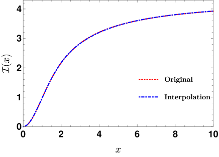
Figure 2: The dotted curve depicts the numerical result for the original integral function whereas the dot-dashed line draws the interpolating function $\mathcal{I}(x)$. Both $x$ and $\mathcal{I}(x)$ are dimensionless. $\mathcal{I}(\infty)$ converges to 4.41625.

Using it, we can solve the Schrödinger equation in an easy manner. The Hamiltonian for the quarkonium system is written by

$$H=-\frac{\hbar^{2}}{m_{Q}}\nabla^{2}+V_{Q\bar{Q}},$$ (74)

where $m_{Q}$ stands for the reduced mass of the heavy-quark and $V_{Q\bar{Q}}$ denotes the $Q\bar{Q}$ potential that consists of

$$V_{Q\bar{Q}} =V_{\rm C}+V_{I}+V_{SD}+V_{SD}^{I}+V_{\rm s}.$$ (75)

Here, $V_{C}$ and $V_{s}$ designate the Coulomb-like and confining potentials, respectively. The linear potential (LP) has often been used for $V_{s}$ [22, 21, 23, 18, 56, 55], since it arises from the Wilson’s area law [16]. However, when a quark continues to separate from an antiquark, the string connecting them will be broken at a certain scale and a light quark-antiquark pair will be created from the vacuum. The LP does not explain this feature of the quark confinement. This makes it difficult to explain the EM transitions for excited states of the charmonia quantitatively. Thus, the strong screened potential for $V_{s}$ was used in Refs. [23], which is saturated as $r$ increases. In the current work, we revise the strong screened potential by introducing the Gaussian function, expressed as

$$V_{\rm s}(r) =k(1-e^{-br^{2}})/b,$$ (76)

which provides a better description of the EM transitions in the presence of the instanton-induced heavy-quark potential. To solve the Schrödinger equation, we use the variational method that minimizes the eigenvalues with the six experimental values of the charmonium masses used as input. Minimizing the eigenvalues, we determine the fitting parameters listed in Table 1. Model I is constructed by excluding the instanton-induced potential, whereas Model II is built by including it.

Table 1: Fitting parameters to minimize the masses of the charmonia. We use the instanton parameters “$\bar{\rho}=1/3$ fm and $R=1$ fm.”

Model	$\alpha_{s}$(-)	$k$(GeV3)	$\sigma$(GeV)	$m_{c}$(GeV)	$b$(GeV2)
Model I	0.5016	0.0324	1.1895	1.5566	0.0244
Model II	0.4863	0.0289	1.2112	1.5358	0.0234

We want to emphasize that with the instanton-induced potential and confining one given in Eq. (76) we can use a value of the one-loop running strong coupling constant close to the physical one at the charm-quark mass scale, which is written by

$$\alpha_{s}(\mu)=\frac{4\pi}{\beta_{0}}\frac{1}{\ln(\mu^{2}/\Lambda^{2}_{QCD})},$$ (77)

where $\beta_{0}=(11N_{c}-2N_{f})/3$, $\Lambda_{\mathrm{QCD}}=0.217$ GeV [57] and the scale $\mu\approx m_{c}$. If $\mu$ is fixed at the charm-quark mass $\mu\thickapprox m_{c}=1.275$ GeV, then $\alpha_{s}(\mu)=0.4258$. Note that this value is closer to that used in the instanton liquid model (see Table 1).

It is of great interest to compare the heavy-quark potential with the instanton effects to the phenomenological potential [21] and that derived from lattice QCD [58]. We draw the central and spin-spin potentials respectively in Figs. 3 and 4. The potentials used for Model I and Model II are illustrated in the solid and dashed curves, whereas those from the NR model and lattice QCD are depicted in the short-dashed and dot-dashed ones, respectively.

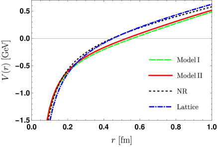
Figure 3: The central part of the $Q\bar{Q}$ potential. The green long-dashed and red solid curves draw the present results, whereas the black short-dashed and blue dash-dotted ones illustrate those from the nonrelativistic model (NR) [21] and lattice QCD [58], respectively.

Figure 4: The spin-spin part of the $Q\bar{Q}$ potential. The notations are the same as in Fig. 3.

In Table 2, the parameters used in the NR approach [21] and lattice QCD [58] are given in Table 2.

Table 2: The parameters of the $Q\bar{Q}$ potential in the NR model [21] and lattice QCD [58].

	$\alpha_{s}$(-)	$\varkappa$(GeV2)	$m_{c}$(GeV)	$\sigma$(GeV)	$A$(GeV)	$B$(GeV2)
NR	0.5461	0.1425	1.4794	1.0946	-	-
LQCD	0.6010	0.1552	1.9888	1.0010	0.314	1.020

Comparing the values of parameters listed in Table 2 with those in Table 1, we find that those of $\alpha_{s}$ used in the NR approach and lattice QCD are larger than the physical one employed in Model II. The charm-quark mass in the present work is larger than that in Ref. [21] but is smaller than in Ref. [58].

The Coulomb-like potential from one-gluon exchange is expressed as

$$V_{\rm C}(r)=-\frac{4\alpha_{s}}{3r}.$$ (78)

In Model II, the contribution from the instanton vacuum is added (see Eq. (75)). The confining potential employed in Model I and Model II is defined in Eq. (76), whereas the NR model and lattice QCD use the linear type $V_{\rm s}=\varkappa r$.

In both Model I and the NR approach, the spin-spin potential given in Eq. (20) are used, whereas in Model II we have additionally Eq. (54). On the other hand, in lattice QCD the following form of the spin-spin potential is adopted

$$V_{SS}=A\exp(-Br^{2}).$$ (79)

We have extracted the values of $m_{c}$ and $\sigma$ in lattice QCD by comparing Eqs. (20) and (79).

One can see that the central parts of all the four potentials in Fig. 3 are more or less the same at small distances. Only at large distances, the potentials in Model I and II become slightly lower than those used in the NR approach and Lattice QCD on account of the screening effect in Eq. (76). The spin-spin part of the present one is similar to that from the NR model but becomes very larger than that from lattice QCD.

As mentioned already, we use the six different values of the charmonium masses as input, which are denoted by the asterisks in the second column of Table 2. Though, in general, the instanton-induced potential provides a marginal contribution to the masses of charmonia, they still improve the numerical results, compared to the experimental data.

Table 3: Numerical results for the charmonium spectrum. The marked with the asterisk denotes the input data we have used to obtain the eigenvalues of the Schrödinger equation. Model I and Model II represent the results of the present work without and with the instanton-induced potential. The columns with the NR and GI list respectively the results from the nonrelativistic linear potential and the Godfrey-Isgur relativized quark model [21]. Those with the LP and SP are taken from Ref. [23] in which both the linear confining potential and screened potential in the form of $(1-e^{-ar})$ are used, respectively.

State	Exp	Model I	Model II	NR [21]	GI [21]	LP [23]	SP [23]
$J/\psi(1^{3}S_{1})$	$3096.900\pm 0.006^{*}$	3064	3097	3090	3098	3097	3097
$\eta_{c}\ (1^{1}S_{0})$	$2983.9\pm 0.4^{*}$	2957	2984	2982	2975	2984	2984
$\psi\ (2^{3}S_{1})$	$3686.097\pm 0.025^{*}$	3620	3687	3672	3676	3679	3679
$\eta_{c}\ (2^{1}S_{0})$	$3637.6\pm 1.1^{*}$	3572	3637	3630	3623	3635	3637
$\psi\ (3^{3}S_{1})$	$4039\pm 1$	4005	4089	4072	4100	4078	4030
$\eta_{c}\ (3^{1}S_{0})$		3976	4060	4043	4064	4048	4004
$\psi\ (4^{3}S_{1})$	$4421\pm 4$	4236	4338	4406	4450	4412	4281
$\eta_{c}\ (4^{1}S_{0})$		4223	4324	4384	4425	4388	4264
$\chi_{c2}\ (1^{3}P_{2})$	$3556.17\pm 0.07^{*}$	3493	3556	3556	3550	3552	3553
$\chi_{c1}\ (1^{3}P_{1})$	$3510.67\pm 0.05$	3454	3511	3505	3510	3516	3521
$\chi_{c0}\ (1^{3}P_{0})$	$3414.71\pm 0.30$	3335	3414	3424	3445	3415	3415
$h_{c}\ (1^{1}P_{1})$	$3525.38\pm 0.11^{*}$	3467	3526	3516	3517	3522	3526
$\chi_{c2}\ (2^{3}P_{2})$	$3922.5\pm 1.0$	3913	3994	3972	3979	3967	3937
$\chi_{c1}\ (2^{3}P_{1})$	$3871.65\pm 0.06$	3879	3956	3925	3953	3937	3914
$\chi_{c0}\ (2^{3}P_{0})$	$3862^{+26+40}_{-32-13}$	3784	3885	3852	3916	3869	3848
$h_{c}\ (2^{1}P_{1})$		3889	3967	3934	3956	3940	3916
$\psi_{3}\ (1^{3}D_{3})$	$3842.7\pm 0.2$	3746	3822	3806	3849	3811	3808
$\psi_{2}\ (1^{3}D_{2})$	$3823.7\pm 0.5$	3743	3817	3800	3838	3807	3807
$\psi\ (1^{3}D_{1})$	$3773.7\pm 0.4$	3727	3799	3785	3819	3787	3792
$\eta_{c2}\ (1^{1}D_{2})$		3742	3817	3799	3837	3806	3805
$\psi_{3}\ (2^{3}D_{3})$		4092	4182	4167	4217	4172	4112
$\psi_{2}\ (2^{3}D_{2})$		4088	4177	4158	4208	4165	4109
$\psi\ (2^{3}D_{1})$	$4191\pm 5$	4070	4157	4142	4194	4144	4095
$\eta_{c2}\ (2^{1}D_{2})$		4087	4177	4158	4208	4164	4108

IV The Electromagnetic Transitions of charmonia

Since we have fixed the parameters for the heavy-quark potential by using the mass spectrum of the charmonia, we are now in a position to discuss the results for their EM transitions. The effective Hamiltonian for the quark-photon EM interaction is given by

$$H_{EM}=-e_{c}|e|\bar{\psi}\gamma^{\mu}A_{\mu}\psi,$$ (80)

where $\psi$ and $A_{\mu}$ denote the quark and photon field operators. Using the EM Hamiltonian, we can compute the E1 and M1 transition matrix elements for the charmonia:

$$\mathcal{M}_{\rm E1}^{fi} =-i\omega_{\gamma}e_{c}|e|\langle f|\vec{r}\cdot\hat{\epsilon}^{*}e^{-i\vec{k}\cdot\vec{r}}|i\rangle,$$ (81)

$$\mathcal{M}^{fi}_{\rm M1} =-i\omega_{\gamma}\frac{e_{c}|e|}{2m_{Q}}\langle f|\vec{\sigma}\cdot(\hat{\epsilon}^{*}\times\hat{k})e^{-i\vec{k}\cdot\vec{r}}|i\rangle,$$ (82)

where the initial and final states are defined as

$$|i\rangle =|n;L,m_{l};s,m_{S};J,m_{J}\rangle$$ (83)

$$|f\rangle =|n^{\prime};L^{\prime},m_{l^{\prime}};S^{\prime},m_{s^{\prime}};J^{\prime},m_{J^{\prime}}\rangle.$$ (84)

The E1 and M1 radiative partial widths are defined by Ref. [21]:

$$\Gamma_{\rm E1} (n^{2S+1}L_{J}\rightarrow n^{\prime 2S^{\prime}+1}L^{\prime}_{J^{\prime}}+\gamma)$$ (85)

$$=\frac{\omega_{\gamma}}{2\pi}|\langle f\,\gamma|\mathcal{M}_{\rm E1}|i\,0\rangle|^{2}\frac{E_{f}^{(c\bar{c})}}{M_{i}^{(c\bar{c})}}$$ (86)

$$=\frac{4}{3}C_{fi}\delta_{SS^{\prime}}e_{c}^{2}\alpha|\langle\psi_{f}|r|\psi_{i}\rangle|^{2}E_{\gamma}^{3}\frac{E_{f}^{(c\bar{c})}}{M_{i}^{(c\bar{c})}},$$ (87)

$$\Gamma_{\rm M1} (n^{2S+1}L_{J}\rightarrow n^{\prime 2S^{\prime}+1}L_{J^{\prime}}^{\prime}+\gamma)$$ (88)

$$=\frac{\omega_{\gamma}}{2\pi}|\langle f\,\gamma|\mathcal{M}_{\rm M1}|i\,0\rangle|^{2}\frac{E_{f}^{(c\bar{c})}}{M_{i}^{(c\bar{c})}}$$ (89)

$$=\frac{4}{3}\frac{2J^{\prime}+1}{2L+1}\delta_{LL^{\prime}}\delta_{S,S^{\prime}\pm 1}$$ (90)

$$\qquad\times e_{c}^{2}\frac{\alpha}{m_{c}^{2}}|\langle\psi_{f}|\psi_{i}\rangle|^{2}E_{\gamma}^{3}\frac{E_{f}^{(c\bar{c})}}{M_{i}^{(c\bar{c})}},$$ (91)

where $E_{\gamma}$ represents the energy of the photon, $E_{f}^{(c\bar{c})}$ stands for the energy of the final $c\bar{c}$ state, $M_{i}^{(c\bar{c})}$ is the mass of the initial $c\bar{c}$ state, and $C_{fi}$ is defined as

$$C_{fi}={\rm max}(L,L^{\prime})(2J^{\prime}+1)\left\{\begin{array}[]{ccc}L^{\prime}&J^{\prime}&S\\ J&L&1\end{array}\right\}^{2}.$$ (94)

$\alpha$ denotes the fine-structure constant. $E_{\gamma}$ and $E_{f}^{(c\bar{c})}$ are given as

$$E_{\gamma} =\frac{M_{i}^{2}-M_{f}^{2}}{2M_{i}},$$ (95)

$$E_{f}^{c\bar{c}} =M_{i}-\frac{M_{i}^{2}-M_{f}^{2}}{2M_{i}}.$$ (96)

In Eq. (87) and Eq. (91), $E_{f}^{c\bar{c}}/M_{i}^{c\bar{c}}$ is introduced as the relativistic phase space factor [21]. The wave functions for the charmonium states $\psi_{i}$ and $\psi_{f}$ are obtained by solving the Schrödinger equation with the heavy-quark potential.

Table 4: Decay widths for 2S$\rightarrow$1P. Model I and Model II represent the results of the present work without and with the instanton-induced potential. The columns with the NR and GI list respectively the results from the nonrelativistic linear potential and the Godfrey-Isgur relativized quark model [21]. Those with the LP and SP are taken from Ref. [23] in which both the linear confining potential and screened potential in the form of $(1-e^{-ar})$ are used, respectively. The decay rate is given in unit of keV.

E1 transition
Initial	Final	Model		[21]		[23]		PDG [57]
		I	II	NR	GI	LP	SP	Exp.
$\psi(2^{3}S_{1})$	$\chi_{c2}(1^{3}P_{2})$	40	41	38	24	36	44	$28\pm 1$
	$\chi_{c1}(1^{3}P_{1})$	42	43	54	29	45	48	$29\pm 1$
	$\chi_{c0}(1^{3}P_{0})$	28	28	63	26	27	26	$29\pm 1$
$\eta_{c}(2^{1}S_{0})$	$h_{c}(1^{1}P_{1})$	43	41	49	36	49	52	-

In Table 4, we list the results for the E1 transition from the 2S to 1P states. As shown from those listed in the third and fourth columns, the instanton effects reduce the strengths of the decay rates for $\psi(2^{3}S_{1})\to\chi_{c1,c2}(1^{3}P_{0,1,2})$ but the results are still larger than the experimental data [57]. On the other hand, they do not contribute to its decay to $\chi_{c0}$ and $h_{c}$ almost at all and are in good agreement with the data.

Table 5: Decay widths for 1P$\rightarrow$1S. Notations are the same as in Table 4.

E1 transition
Initial	Final	Model		[21]		[23]		PDG [57]
		I	II	NR	GI	LP	SP	Exp.
$\chi_{c2}(1P)$	$J/\psi(1S)$	388	394	424	313	327	338	$374\pm 19$
$\chi_{c1}(1P)$		311	315	314	239	269	278	$288\pm 16$
$\chi_{c0}(1P)$		146	152	152	114	141	146	$151\pm 12$
$h_{c}(1P)$	$\eta_{c}(1S)$	445	452	498	352	361	373	$350\pm 210$

Table 5 lists the results for the E1 transition from the 1P to 1S states. In contrast to the E1 transitions for $\mathrm{2S}\to\mathrm{1P}$ decays, the instanton effects slightly enhance the decay widths. The decay widths for the $\chi_{cJ}(1P)\to J/\psi(1S)$ are well described by the present heavy-quark potential. That for the $h_{c}(1P)\to\eta_{c}(1S)$ is overestimated, compared with the data.

Table 6: Decay widths for 1D$\rightarrow$1P. Notations are the same as in Table 4.

E1 transition
Initial	Final	Model		[21]		[23]		PDG [57]
		I	II	NR	GI	LP	SP	Exp.
$\psi_{3}(1^{3}D_{3})$	$\chi_{c2}(1^{3}P_{2})$	331	333	272	296	377	393	-
$\psi_{2}(1^{3}D_{2})$		80	80	64	66	79	82	-
	$\chi_{c1}(1^{3}P_{1})$	311	311	307	268	281	291	-
$\psi(1^{3}D_{1})$	$\chi_{c2}(1^{3}P_{2})$	7.2	7.2	4.9	3.3	5.4	5.7	$\leq 17$
	$\chi_{c1}(1^{3}P_{1})$	147	147	125	77	115	111	$68\pm 7$
	$\chi_{c0}(1^{3}P_{0})$	317	315	403	213	243	232	$188\pm 18$

In Table 6, we present the results for the $1\rm D\rightarrow 1P$ decay widths. The decay rates for the $\psi(1^{3}D_{1})\to\chi_{c0,c1}(1^{3}P_{0,1})$ are overestimated, compared with the data. The instanton effects are again very small. Note that the $\psi(3770)$ resonance lies just above the open-charm $D\bar{D}$ threshold. It implies that the light quarks may come into play. Furthermore, the $1^{3}D_{1}$ state $\psi(3770)$ is assumed to be mixed with a small $2^{3}S_{1}$ state [59, 60]. One can improve the results by considering the light-quark contributions and $S-D$ mixing. Since the $\psi(3770)$ is above the $D\bar{D}$ threshold, relativistic corrections may also be important. However, since we aim at the effects of the heavy-quark potential from the instanton vacuum in the current work, we have not considered taken them.

Table 7: Decay widths for the M1 transition. Notations are the same as in Table 4.

M1 transition
Initial	Final	Model		[21]		[23]		PDG [57]
		I	II	NR	GI	LP	SP	Exp.
$J/\psi(1S)$	$\eta_{c}(1S)$	2.5	2.3	2.9	2.4	2.39	2.44	$1.7\pm 0.4$
$\psi(2S)$	$\eta_{c}(2S)$	0.2	0.2	0.21	0.17	0.19	0.19	$0.2\pm 0.2$
	$\eta_{c}(1S)$	5.4	5.0	4.6	9.6	8.08	7.80	$1.0\pm 0.1$
$\eta_{c}(2S)$	$J/\psi(1S)$	9.6	9.0	7.9	5.6	2.64	2.29	$<158$

In Table 7, we list the results for the decay rates for the M1 transition. Though the results describe the experimental data well, the instanton effects are again negligibly small.

V Summary

In the current work, we examined the instanton effects on the mass spectrum and electromagnetic transitions of charmonia. We briefly reviewed how the heavy-quark potential from the instanton vacuum. To improve the results, we introduced a new type of the confining potential. We utilized the experimental data for the masses of the six different charmonia to fit the data. Though the instanton effects are marginal on the mass spectrum of the charmonia, they allow one to use smaller values of the strong coupling constant and the charm-quark mass, which are closer to the physical values compared to other works. Using the effective Hamiltonian for the quark-photon electromagnetic interaction, we derived the radiative decay rates for the E1 and M1 transitions. The instanton heavy-quark potential has generally minor effects on the radiative decays of the charmonia.

References

- [1] E. Eichten, S. Godfrey, H. Mahlke and J. L. Rosner, Rev. Mod. Phys. 80, 1161 (2008).
- [2] M. B. Voloshin, Prog. Part. Nucl. Phys., 61, 455 (2008).
- [3] N. Brambilla, S. Eidelman, B. K. Heltsley, R. Vogt, G. T. Bodwin, E. Eichten, A. D. Frawley, A. B. Meyer, R. E. Mitchell and V. Papadimitriou, et al. Eur. Phys. J. C 71, 1534 (2011).
- [4] C. Patrignani, T. K. Pedlar and J. L. Rosner, Ann. Rev. Nucl. Part. Sci., 63, 21 (2013).
- [5] E. Eichten, K. Gottfried, T. Kinoshita, J. B. Kogut, K. D. Lane and T. M. Yan, Phys. Rev. Lett. 34 (1975) 369 [Phys. Rev. Lett. 36 (1976) 1276].
- [6] E. Eichten, K. Gottfried, T. Kinoshita, K. D. Lane and T. M. Yan, Phys. Rev. D 17 (1978) 3090 [Phys. Rev. D 21 (1980) 313].
- [7] L. Susskind, “Coarse Grained Quantum Chromodynamics,” in Weak and Electromagnetic Interactions at high energies: Proceedings. Edited by Roger Balian and Christopher H. Llewellyn Smith (N.Y., North-Holland, 1977).
- [8] T. Appelquist, M. Dine and I. J. Muzinich, Phys. Lett. B 69 (1977) 231.
- [9] T. Appelquist, M. Dine and I. J. Muzinich, Phys. Rev. D 17 (1978) 2074.
- [10] W. Fischler, Nucl. Phys. B 129 (1977) 157.
- [11] M. Peter, Phys. Rev. Lett. 78 (1997) 602.
- [12] M. Peter, Nucl. Phys. B 501 (1997) 471.
- [13] Y. Schroder, Phys. Lett. B 447 (1999) 321.
- [14] A. V. Smirnov, V. A. Smirnov and M. Steinhauser, Phys. Rev. Lett. 104 (2010) 112002.
- [15] C. Anzai, Y. Kiyo and Y. Sumino, Phys. Rev. Lett. 104 (2010) 112003.
- [16] K. G. Wilson, Phys. Rev. D 10 (1974) 2445.
- [17] D. Diakonov, V. Y. Petrov and P. V. Pobylitsa, Phys. Lett. B 226 (1989) 372.
- [18] U. T. Yakhshiev, H. C. Kim, M. M. Musakhanov, E. Hiyama and B. Turimov, Chin. Phys. C 41 (2017) 083102.
- [19] U. T. Yakhshiev, H.-Ch. Kim and E. Hiyama, Phys. Rev. D 98 (2018) 114036.
- [20] M. Musakhanov and U. Yakhshiev, Int. J. Mod. Phys. E 30 (2021) 2141005.
- [21] T. Barnes, S. Godfrey and E. S. Swanson, Phys. Rev. D 72, 054026 (2005).
- [22] S. Godfrey and N. Isgur, Phys. Rev. D 32, 189 (1985).
- [23] W. J. Deng, H. Liu, L. C. Gui and X. H. Zhong, Phys. Rev. D 95, 034026 (2017).
- [24] E. Laermann, F. Langhammer, I. Schmitt and P. M. Zerwas, Phys. Lett. B 173, 437 (1986).
- [25] K. D. Born, E. Laermann, N. Pirch, T. F. Walsh and P. M. Zerwas, Phys. Rev. D 40, 1653 (1989).
- [26] B. Q. Li and K. T. Chao, Phys. Rev. D 79, 094004 (2009).
- [27] T. Barnes and S. Godfrey, Phys. Rev. D 69, 054008 (2004).
- [28] J. J. Dudek, R. G. Edwards and D. G. Richards, Phys. Rev. D 73, 074507 (2006).
- [29] J. J. Dudek, R. Edwards and C. E. Thomas, Phys. Rev. D 79, 094504 (2009).
- [30] Y. Chen, D. C. Du, B. Z. Guo, N. Li, C. Liu, H. Liu, Y. B. Liu, J. P. Ma, X. F. Meng and Z. Y. Niu, et al. Phys. Rev. D 84, 034503 (2011).
- [31] Y. B. Yang et al. [CLQCD], Phys. Rev. D 87, 014501 (2013).
- [32] G. C. Donald, C. T. H. Davies, R. J. Dowdall, E. Follana, K. Hornbostel, J. Koponen, G. P. Lepage and C. McNeile, Phys. Rev. D 86, 094501 (2012).
- [33] D. Bečirević, M. Kruse and F. Sanfilippo, JHEP 05, 014 (2015).
- [34] V. A. Beilin and A. V. Radyushkin, Nucl. Phys. B 260, 61 (1985).
- [35] S. P. Guo, Y. J. Sun, W. Hong, Q. Huang and G. H. Zhao, Nucl. Phys. B 955, 115053 (2020).
- [36] H. D. Li, C. D. Lü, C. Wang, Y. M. Wang and Y. B. Wei, JHEP 04, 023 (2020).
- [37] S. Bhatnagar and E. Gebrehana, Phys. Rev. D 102, 094024 (2020).
- [38] V. Guleria, E. Gebrehana and S. Bhatnagar, Phys. Rev. D 104, 094045 (2021).
- [39] N. Brambilla, Y. Jia and A. Vairo, Phys. Rev. D 73, 054005 (2006).
- [40] A. Pineda and J. Segovia, Phys. Rev. D 87, 074024 (2013).
- [41] H. W. Ke, X. Q. Li and Y. L. Shi, Phys. Rev. D 87, 054022 (2013).
- [42] P. Guo, T. Yépez-Martínez and A. P. Szczepaniak, Phys. Rev. D 89, 116005 (2014).
- [43] Y. L. Shi, Eur. Phys. J. C 77, 253 (2017).
- [44] M. Li, Y. Li, P. Maris and J. P. Vary, Phys. Rev. D 98, 034024 (2018).
- [45] G. Ganbold, T. Gutsche, M. A. Ivanov and V. E. Lyubovitskij, Phys. Rev. D 104, 094048 (2021).
- [46] E. V. Shuryak, Nucl. Phys. B 203, 140 (1982).
- [47] D. Diakonov and V. Y. Petrov, Nucl. Phys. B 245, 259 (1984).
- [48] D. Diakonov and V. Y. Petrov, Nucl. Phys. B 272, 457 (1986).
- [49] M. Musakhanov, N. Rakhimov and U. T. Yakhshiev, Phys. Rev. D 102 (2020) 076022.
- [50] P. Pobylitsa Phys. Lett. B 226 (1989) 387.
- [51] E. Eichten and F. Feinberg, Phys. Rev. D 23 (1981) 2724.
- [52] B. Pandya, M. Shah and P. C. Vinodkumar, DAE Symp. Nucl. Phys. 63, 838 (2018).
- [53] P. P. D’Souza, A. P. Monteiro and K. B. Vijay Kumar, DAE Symp. Nucl. Phys. 63, 850 (2018).
- [54] A. E. Dorokhov, N. I. Kochelev, S. V. Molodtsov and G. M. Zinovev, Phys. Atom. Nucl. 70, 938 (2007).
- [55] P. P D’Souza, A. Prakash Monteiro and K. B. Vijaya Kumar, Commun. Theor. Phys. 71, 192 (2019).
- [56] U. Yakhshiev, J. Korean Phys. Soc. 79 (2021) 357.
- [57] R. L. Workman [Particle Data Group], PTEP 2022, 083C01 (2022).
- [58] T. Kawanai and S. Sasaki, Phys. Rev. D 85, 091503 (2012).
- [59] J. L. Rosner, Phys. Rev. D 64, 094002 (2001).
- [60] J. L. Rosner, Annals Phys. 319, 1 (2005).