Bose-Einstein-Like condensation of deformed random matrix: A replica approach

Abstract

In this work, we investigate a symmetric deformed random matrix, which is obtained by perturbing the diagonal elements of the Wigner matrix. The eigenvector $\bm{x}_{\rm min}$ of the minimal eigenvalue $\lambda_{\rm min}$ of the deformed random matrix tends to condensate at a single site. In certain types of perturbations and in the limit of the large components, this condensation becomes a sharp phase transition, the mechanism of which can be identified with the Bose-Einstein condensation in a mathematical level. We study this Bose-Einstein like condensation phenomenon by means of the replica method. We first derive a formula to calculate the minimal eigenvalue and the statistical properties of $\bm{x}_{\rm min}$. Then, we apply the formula for two solvable cases: when the distribution of the perturbation has the double peak, and when it has a continuous distribution. For the double peak, we find that at the transition point, the participation ratio changes discontinuously from a finite value to zero. On the contrary, in the case of a continuous distribution, the participation ratio goes to zero either continuously or discontinuously, depending on the distribution.

1 Introduction

In this manuscript, we study the eigenvector $\bm{x}_{\rm min}$ of the minimal eigenvalue $\lambda_{\rm min}$ of the deformed Wigner matrix, where the $i$-th diagonal element of the Wigner matrix is perturbed by a constant $h_{i}$ [1, 2, 3, 4, 5]. When $\left|h_{i}\right|\ll 1$, all components of $\bm{x}_{\rm min}$ have the same order of magnitude, as in the case of the original Wigner matrix [6]. On the contrary, when $\left|h_{i}\right|\gg 1$, $\bm{x}_{\rm min}$ tends to condensate at the site with the smallest $h_{i}$ [5]. For some specific distributions of $h_{i}$, the condensation becomes a sharp phase transition in the limit of the large number of components [2]. Interestingly, this condensation transition has a similar mathematical structure of that of the Bose-Einstein condensation [7, 2, 8, 9].

The deformed random matrix has been used to understand complex atomic spectra [1], Anderson Localization [2], principal component analysis [10], and so on [11]. Recently the model has gained renewed interest as a toy model to describe the vibrational properties of amorphous solids [8, 9, 12, 13]. Several numerical studies uncovered that in addition to the usual phonon modes, there appear many quasi-localized modes in low-frequency vibrational density of states of amorphous solids [14, 15, 16, 17]. In particular, the participation ratio of the quasi-localized mode of the lowest frequency is inversely proportional to the system size, meaning that the eigenvector of the minimal eigenvalue of the Hessian of an amorphous solid is localized [14]. The result contradicts a mean-field theory of the glass transition, where a Hessian of an amorphous solid is approximated by a dense random matrix, whose eigenvectors are extended [18, 19]. To reconcile this discrepancy, Rainone et al. [12, 13, 20] recently introduced a mean-field model whose effective Hessian in the RS phase can be considered as a deformed random matrix. The model exhibits the localization transition at which the eigenvector of the minimal eigenvalue is localized. Thus it correctly reproduces the localized property of amorphous solids. More recently, Franz et al. studied a fully-connected vector spin-glass model and found similar localization of the eigenvector of the lowest frequency [8, 9]. They also pointed out that this localization is caused by a Bose-Einstein (like) condensation [8, 9].

Motivated by those recent developments of disordered systems, here we investigate a replica method to describe the Bose-Einstein like condensation of the minimal eigenvector of the deformed random matrix. The replica method is a powerful tool to treat disordered systems such as spin-glass [21], amorphous solids, and granular materials [22]. This is also true in the field of random matrices [6]. A seminar work has been done by Edwards and Jones in Ref [23]. They studied a symmetric random matrix in which each element follows a Gaussian distribution of zero mean and fixed variance. By using the replica method, they showed that the eigenvalue distribution of the matrix converges to the well-known Wigner semicircle distribution [6]. Later, the replica method was also applied to calculate the eigenvalue distribution of an asymmetric random matrix [24], symmetric sparse random matrix [25, 26, 27, 28], and so on. We here show that the replica method is also useful for the analysis of the lowest eigenmode of the deformed random matrix.

The structure of the paper is as follows. In Sec. 2, we describe the model. In Sec. 3, we describe how to calculate the minimal eigenvalue and eigenvector by using the replica method. In Sec. 4, we present the results. In Sec. 5, we conclude the work.

2 Model

We consider a $N\times N$ symmetric matrix whose $ij$ component is written as

$$W_{ij}=J_{ij}+h_{i}\delta_{ij}.$$ (1)

Here $J_{ij}=J_{ji}$ is a i.i.d random variable following a Gaussian distribution

$$P(J_{ij})=\sqrt{\frac{N}{2\pi}}e^{-\frac{NJ_{ij}^{2}}{2}},$$ (2)

and $\{h_{i}\}_{i=1,\dots,N}$ are constants. Unfortunately, our present method does not work for general values of $h_{i}$’s. We restrict our analysis for a specific case [29]:

$$h_{i}=\begin{cases}h_{1}&(i=1,\dots,N/M),\\ \vdots\\ h_{k}&(i=kN/M+1,\dots,(k+1)N/M),\\ \vdots\\ h_{M}&(i=N-N/M+1,\dots,N).\\ \end{cases}$$ (3)

By setting $h_{i}$ this way, we can define an overlap $q_{k}$ corresponding to each $h_{k}$, which quantifies how much the eigenvector is condensed/localized to the sites perturbed by $h_{k}$. At the end of the calculation, we take the $M\to\infty$ limit, but even there we require that $N/M$ goes to infinity. To be more specific, we first take the thermodynamic limit $N\to\infty$ and then take the limit $M\to\infty$.

3 Theory

3.1 Interaction potential and ground state

Here we use the method developed by Kabashima and Takahashi [30]. To investigate the minimal eigenvalue $\lambda_{\rm min}$ and corresponding vector $\bm{x}_{\rm min}$ of $W$, we consider a system interacting with the following potential:

$$H(\bm{x}|J) \equiv\frac{\bm{x}\cdot W\cdot\bm{x}}{2}$$

$$=\frac{\bm{x}\cdot J\cdot\bm{x}}{2}+\frac{1}{2}\sum_{k=1}^{M}h_{k}\bm{x}_{k}\cdot\bm{x}_{k},$$ (4)

where the $N$ dimensional vector $\bm{x}=\{x_{1},\dots,x_{N}\}$ denotes the state variable. We also introduced the sub-vectors:

$$\bm{x}_{k}=\{x_{i}\}_{i=k\frac{N}{M}+1,\dots,(k+1)\frac{N}{M}}.$$ (5)

We impose that the state vector $\bm{x}$ satisfies the spherical constraint:

$$\bm{x}\cdot\bm{x}=\sum_{k=1}^{M}\bm{x}_{k}\cdot\bm{x}_{k}=\sum_{i=1}^{N}x_{i}^{2}=N.$$ (6)

When $h_{i}=0$, the model Eq. (4) can be identified with the $p=2$ spin spherical model, which has been fully investigated before [31, 32, 33].

Under the above setup, it is easy to show that when $\bm{x}=\bm{x}_{\rm min}$, we get the ground state energy [30, 34]:

$$H_{\rm GS}=\frac{\bm{x}_{\rm min}\cdot W\cdot\bm{x}_{\rm min}}{2}=\frac{\lambda_{\rm min}}{2}N.$$ (7)

Therefore, the minimal eigenvalue is calculated as $\lambda_{\rm min}=2H_{\rm GS}/N$.

3.2 Replica method

To investigate the ground state, we introduce the partition function [30]:

$$Z(J)=\int d\bm{x}\delta(\bm{x}\cdot\bm{x}-N)e^{-\beta H(\bm{x}|J)}$$ (8)

and the free-energy

$$-\beta f=\frac{1}{N}\overline{\log Z(J)},$$ (9)

where $\beta=1/T$ denotes the inverse temperature, and the overline denotes the average for the quenched randomness $J$. The ground state energy per particle is given by taking the zero temperature limit of the free-energy

$$e_{\rm GS}\equiv\frac{H_{\rm GS}}{N}=\lim_{T\to 0}f.$$ (10)

Below we omit the subscript ${\rm GS}$ unless it causes confusion. To perform the disordered average in Eq. (9), we use the replica trick [21]:

$$-\beta f=\lim_{n\to 0}\frac{\log\overline{Z(J)^{n}}}{nN},$$ (11)

where we have introduced the replicated partition function as follows:

$$\overline{Z^{n}}=\int\prod_{a=1}^{n}d\bm{x}_{a}\delta(\bm{x}_{a}\cdot\bm{x}_{a}-N)\overline{e^{-\beta\sum_{a=1}^{n}H(\bm{x}_{a}|J)}}.$$ (12)

Since the distribution of $J_{ij}$ is a Gaussian Eq. (2), the quenched average can be taken analytically [18] :

$$\overline{e^{-\beta\sum_{a=1}^{n}H(\bm{x}_{a}|J)}}\sim\exp\left[\frac{N\beta^{2}}{4}\sum_{ab}Q^{ab}-\frac{\beta}{2M}\sum_{a=1}^{n}\sum_{k=1}^{M}h_{k}Q_{k}^{aa}\right],$$ (13)

where we have defined the overlaps as follows:

$$Q_{k}^{ab}\equiv\frac{\bm{x}_{k}^{a}\cdot\bm{x}_{k}^{b}}{N/M},$$

$$Q_{ab}\equiv\frac{1}{M}\sum_{k=1}^{M}Q_{k}^{ab}=\frac{1}{N}\sum_{i=1}^{N}x_{i}^{a}x_{i}^{b}.$$ (14)

When we change the variable from $\{\bm{x}_{k}^{a}\}_{a=1,\dots,n}$ to $\{Q_{k}^{ab}\}_{a,b=1,\dots n}$, the following Jacobian apepars [35]:

$$\prod_{a=1}^{n}\int d\bm{x}_{k}^{a}=\prod_{a=1}^{n}\int d\bm{x}_{k}^{a}\prod_{ab}\int dQ_{k}^{ab}\delta\left(\frac{N}{M}Q_{k}^{ab}-\bm{x}_{k}^{a}\cdot\bm{x}_{k}^{b}\right)\sim\prod_{ab}\int dQ_{k}^{ab}e^{\frac{N}{2M}\log\det Q_{k}}.$$ (15)

Summarizing the above results, we get

$$\overline{Z^{n}}=\prod_{k,a,b}\int dQ_{k}^{ab}e^{NS(Q)},$$ (16)

where

$$S(Q) =\frac{1}{2M}\sum_{k=1}^{M}\log\det Q_{k}+\frac{\beta^{2}}{4}\sum_{ab}\left(Q^{ab}\right)^{2}-\beta\frac{1}{2M}\sum_{a=1}^{n}\sum_{k=1}^{M}h_{k}Q_{k}^{aa}.$$ (17)

We should minimize $S(Q)$ with the spherical constraint

$$Q^{aa}=\frac{1}{M}\sum_{k=1}^{M}Q_{k}^{aa}=1,\ a=1,\dots,n.$$ (18)

To proceed the calculation, we assume the replica symmetric Ansatz [21]:

$$Q_{k}^{ab}=\delta_{ab}q_{k}+(1-\delta_{ab})p_{k}.$$ (19)

Then, we get

$$S(Q) =\frac{1}{M}\sum_{k=1}^{M}\frac{1}{2}\left[\log(q_{k}+(n-1)p_{k})+(n-1)\log(q_{k}-p_{k})\right]$$

$$+\frac{\beta^{2}}{4}\left(n+n(n-1)p^{2}\right)-n\frac{\beta}{2M}\sum_{k=1}^{M}h_{k}q_{k},$$ (20)

where

$$p=\frac{1}{M}\sum_{k=1}^{M}p_{k}.$$ (21)

Finally, by taking the $n\to 0$ limit, we get the free-energy

$$-\beta f =\lim_{n\to 0}\frac{\log\overline{Z^{n}}}{nN}=\lim_{n\to 0}\frac{S(Q)}{n}$$

$$=\frac{1}{2M}\sum_{k=1}^{M}\left[\frac{p_{k}}{q_{k}-p_{k}}+\log(q_{k}-p_{k})\right]+\frac{\beta^{2}}{4}(1-p^{2})-\frac{\beta}{2M}\sum_{k=1}^{M}h_{k}q_{k}.$$ (22)

3.3 Ground state energy

To get the ground state energy, we should take the zero temperature limit $T\to 0$. This is possible by using the harmonic approximation:

$$T\chi_{k}=q_{k}-p_{k},$$ (23)

which is validated at sufficiently low $T$ [35]. Substituting Eq. (23) into Eq. (22) and taking $T\to 0$ limit, we get

$$e=\lim_{T\to 0}f=-\frac{1}{2M}\sum_{k=1}^{M}\frac{q_{k}}{\chi_{k}}-\frac{\chi}{2}+\frac{1}{2M}\sum_{k=1}^{M}h_{k}q_{k},$$ (24)

where

$$\chi=\frac{1}{M}\sum_{k=1}^{M}\chi_{k}.$$ (25)

Now we minimize it for $\chi_{k}$ and $q_{k}$. We first consider the saddle point condition for $\chi_{k}$:

$$\frac{\partial e}{\partial\chi_{k}}=\frac{q_{k}}{2M\chi_{k}^{2}}-\frac{1}{2M}=0\to\chi_{k}=\sqrt{q_{k}}.$$ (26)

Using this equation, one can eliminate $\chi_{k}$ from Eq. (24):

$$e =-\frac{1}{2M}\sum_{k=1}^{M}\sqrt{q_{k}}-\frac{1}{2M}\sum_{k=1}^{M}\sqrt{q_{k}}+\frac{1}{2M}\sum_{k=1}^{M}h_{k}q_{k}$$

$$=-\frac{1}{M}\sum_{k=1}^{M}\sqrt{q_{k}}+\frac{1}{2M}\sum_{k=1}^{M}h_{k}q_{k}.$$ (27)

Next, we should minimize $e$ w.r.t $q_{k}$ with the spherical constraint $q=\sum_{k=1}^{M}q_{k}/M=1$. To this purpose, we introduce the Lagrange multiplier $\mu$:

$$e =-\frac{1}{M}\sum_{k=1}^{M}\sqrt{q_{k}}+\frac{1}{2M}\sum_{k=1}^{M}h_{k}q_{k}+\frac{\mu}{2M}\left(\sum_{k=1}^{M}q_{k}-M\right).$$ (28)

The saddle point condition for $q_{k}$ leads to

$$\frac{\partial e}{\partial q_{k}}=-\frac{1}{2M\sqrt{q_{k}}}+\frac{h_{k}+\mu}{2M}=0\to\sqrt{q_{k}}=\frac{1}{\mu+h_{k}}.$$ (29)

Since $\sqrt{q_{k}}\geq 0$, $\mu$ should satisfy

$$\mu+\min_{k}h_{k}\geq 0.$$ (30)

The Lagrange multiplier $\mu$ should be determined by the following condition:

$$1=\frac{1}{M}\sum_{k=1}^{M}q_{k}=\frac{1}{M}\sum_{k=1}^{M}\frac{1}{(\mu+h_{k})^{2}}=\int_{-\infty}^{\infty}dhP(h)q(h),$$ (31)

where we have introduced the distribution of $h_{k}$

$$P(h)=\frac{1}{M}\sum_{k=1}^{M}\delta(h-h_{k}),$$ (32)

and the self-overlap of spins subjected to the external field $h$

$$q(h)=\frac{1}{(\mu+h)^{2}}.$$ (33)

Similar equations as Eq. (31) have been previously obtained for a sparse random matrix [30] and deformed random matrices [8, 9, 11]. Substituting the above results into Eq. (7), one can calculate $\lambda_{\rm min}$ as follows:

$$\lambda_{\rm min} =\frac{2H_{\rm GS}}{N}=2e$$

$$=2\int_{-\infty}^{\infty}dhP(h)\left[\frac{hq(h)}{2}-\sqrt{q(h)}\right]$$

$$=2\int_{-\infty}^{\infty}dhP(h)\left[\frac{h}{2(h+\mu)^{2}}-\frac{1}{h+\mu}\right].$$ (34)

4 Results

4.1 Single delta peak

We first check the result for a single delta peak:

$$P(h)=\delta(h-\Delta),$$ (35)

which is tantamount to consider the matrix:

$$W=J+\Delta I,$$ (36)

where $I$ is the $N\times N$ identity matrix. The minimal eigenvalue of this matrix is $\lambda_{\rm min}=-2+\Delta$ [6]. Below, we check if our method can correctly reproduce this result.

The spherical constraint Eq. (31) in this case is

$$1=\int_{-\infty}^{\infty}dhP(h)q(h)=q(\Delta)=\frac{1}{(\mu+\Delta)^{2}}.$$ (37)

Solving this equation for $\mu$, we get

$$\mu=1-\Delta.$$ (38)

The minimal eigenvalue is calculated as

$$\lambda_{\rm min}=2e=2\int_{-\infty}^{\infty}dhP(h)\left[\frac{h}{2(h+\mu)^{2}}-\frac{1}{h+\mu}\right]=\frac{\Delta}{(\Delta+\mu)^{2}}-\frac{2}{\Delta+\mu}=\Delta-2.$$ (39)

The known result has been correctly reproduced.

4.2 Binary distribution

Here we consider a simple binary distribution:

$$P(h)=c\delta(h)+(1-c)\delta(h-\Delta),$$ (40)

where $c\in[0,1]$ and $\Delta$ is a positive constant. Assuming the distribution Eq. (40) is tantamount to set the external field in Eq. (3) as

$$h_{i}=\begin{cases}0&i=1,\dots,cN,\\ \Delta&i=cN+1,\dots,N\end{cases}.$$ (41)

Now the spherical constraint Eq. (31) is written as follows

$$1=cq(0)+(1-c)q(\Delta),$$ (42)

where

$$q(0)=\frac{1}{\mu^{2}},\hskip 14.22636ptq(\Delta)=\frac{1}{(\mu+\Delta)^{2}}.$$ (43)

The Lagrange multiplier $\mu$ should be determined so as to satisfy Eq. (42). In Fig. 1, we plot $\mu$ for several $c$. For later comparison with the result of the continuous distribution, we are in particular interested in the limit $c\to 0$. A naive expectation is that Eq. (42) in this limit reduces to

$$1\approx q(\Delta)=\frac{1}{(\mu+\Delta)^{2}}.$$ (44)

Solving this equation, we get

$$\mu=1-\Delta.$$ (45)

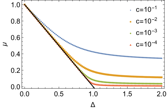
Figure 1: $\Delta$ dependence of the Lagrange multiplier $\mu$ for the binary distribution. Markers denote the results for $c>0$, while the solid line denotes the result in the limit $c\to 0$.

Eq. (45) however implies that $\mu$ becomes negative when $\Delta>1$, which is prohibited by Eq. (30). What was wrong? What we missed is that when $\mu\sim 0$, the first term on the right-hand side of Eq. (42), $cq(0)=c/\mu^{2}$ can no longer be ignored. Let we assume that this term takes a finite value for $\Delta>1$, then from Eq. (42), we get

$$cq(0)=1-\frac{1-c}{(\mu+\Delta)^{2}}\approx 1-\frac{1}{\Delta^{2}}.$$ (46)

From Eqs. (43), (45), and (46), we can deduce the behavior of $\mu$, $q(0)$ and $q(\Delta)$ in the limit $c\to 0$ as follows:

$$\mu=\begin{cases}1-\Delta&(\Delta\leq 1)\\ 0&(\Delta>1)\end{cases}, q(0)=\begin{cases}1/(1-\Delta)^{2}&(\Delta\leq 1)\\ c^{-1}(1-1/\Delta^{2})&(\Delta>1)\end{cases}, q(\Delta)=\begin{cases}1&(\Delta\leq 1)\\ 1/\Delta^{2}&(\Delta>1)\end{cases}.$$ (47)

In Figs. 1 and 2, we plot $\mu$, $q(0)$, and $cq(0)$ for several $c$ to show how these results converge to Eqs. (47) in the limit $c\to 0$.

Figure 2: $\Delta$ dependence of the overlaps for the binary distribution. Markers denote results for $c>0$, while the solid line denotes the result in the limit $c\to 0$.

From Eq. (34), ground state energy is calculated as

$$e=\int_{-\infty}^{\infty}dhP(h)\left[\frac{h}{2(h+\mu)^{2}}-\frac{1}{h+\mu}\right]=-\frac{c}{\mu}+(1-c)\left[\frac{\Delta}{2(\Delta+\mu)^{2}}-\frac{1}{\Delta+\mu}\right].$$ (48)

Substituting Eqs. (47) into the above equation, we get in the limit $c\to 0$

$$\lambda_{\rm min}=2e\to\begin{cases}\Delta-2&(\Delta\leq 1),\\ -1/\Delta&(\Delta>1).\end{cases}$$ (49)

In Fig. 3, we plot this equation with the results of finite $c$’s.

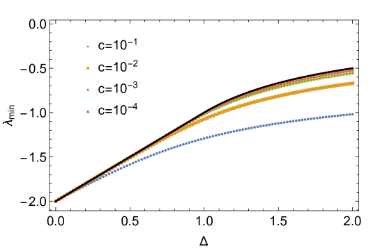
Figure 3: $\Delta$ dependence of the minimal eigenvalue $\lambda_{\rm min}$ for the binary distribution. Markers denote results for $c>0$, while the solid line denotes the result in the limit $c\to 0$.

Now we discuss the degree of the localization. For this purpose, we define the participation ratio:

$${\rm PR}\equiv\frac{1}{N}\frac{(\sum_{i=1}^{N}\left\langle x_{i}^{2}\right\rangle)^{2}}{\sum_{i=1}^{N}\left\langle x_{i}^{4}\right\rangle}=\left[\frac{1}{N}\sum_{i=1}^{N}\left\langle x_{i}^{4}\right\rangle\right]^{-1},$$ (50)

where

$$\left\langle O\right\rangle\equiv\lim_{T\to 0}\frac{\int d\bm{x}e^{-\beta H}O}{\int d\bm{x}e^{-\beta H}}.$$ (51)

The partition ratio takes ${\rm PR}=O(1)$ when $\bm{x}$ is extended, while ${\rm PR}=0$ when $\bm{x}$ is localized. To calculate the forth moment of $x_{i}$, we assume that $x_{i}$ follows the normal distribution of zero mean and variance $q(0)$ for $i\leq cN$ and variance $q(\Delta)$ for $i>cN$ [8]. Then, we get

$$\left\langle x_{i}^{4}\right\rangle\approx 3\left\langle x_{i}\right\rangle^{2}=\begin{cases}3q(0)^{2}&i=1,\dots,cN\\ 3q(\Delta)^{2}&i=cN+1,\dots,N\end{cases}.$$ (52)

In the limit $c\to 0$, Eq. (50) reduces to

$${\rm PR}(\Delta)=\frac{1}{3}\frac{1}{cq(0)^{2}+(1-c)q(\Delta)^{2}}\to\begin{cases}1/3&(\Delta\leq 1)\\ 0&(\Delta>1).\end{cases}$$ (53)

Therefore, the eigenvector of the minimal eigenvalue is localized for $\Delta>1$.

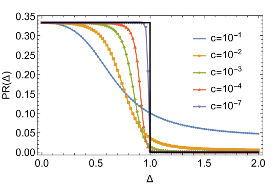
Figure 4: $\Delta$ dependence of the participation ratio ${\rm PR}$ for the binary distribution. Markers denote results for $c>0$, while the solid line denotes the result for $c=0$.

In Fig. 4, we plot ${\rm PR}$ for several $c$ to see how the results converge to Eq. (53) in the limit $c\to 0$.

4.3 Continuous distribution: Bose-Einstein condensation

In the limit $M\to\infty$, one expects that $P(h)$ is approximated by a continuous function. To simplify the calculation, here we only consider the following function:

$$P(h)=\begin{cases}(1+n)h^{n}/\Delta^{1+n}&h\in[0,\Delta],\\ 0&{\rm otherwise}\end{cases},$$ (54)

where $\Delta$ is a positive constant. The pre-factor has been chosen so that $\int_{-\infty}^{\infty}dhP(h)=1$. The Lagrange multiplier is determined by the spherical constraint:

$$1=\int_{-\infty}^{\infty}dhP(h)q(h)=\frac{(1+n)}{\Delta^{n+1}}\int_{0}^{\Delta}\frac{h^{n}dh}{(h+\mu)^{2}}.$$ (55)

In Fig. 5, we plot the results for several $n$.

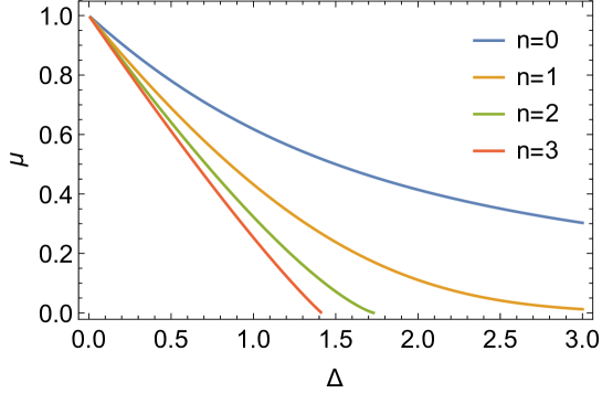
Figure 5: $\Delta$ dependence of the Lagrange multipliyer for the continuous distribution. For $n>1$, we plot the data only for $\Delta\leq\Delta_{c}$.

The integral in Eq. (55) takes a maximum at $\mu=0$ ($\mu$ can not be negative due to Eq. (30)). If $n>1$, the integral at $\mu=0$ converges to a finite value :

$$\frac{1+n}{\Delta^{n+1}}\int_{0}^{\Delta}h^{n-2}dh=\frac{n+1}{\Delta^{2}(n-1)}.$$ (56)

When $1>\Delta^{-2}(n+1)/(n-1)$ or equivalently

$$\Delta>\Delta_{c}\equiv\sqrt{\frac{n+1}{n-1}},$$ (57)

Eq. (55) has no solution. This is similar to the situation of the previous section, and the term corresponding to $h_{k}=0$ should be carefully treated. For this purpose, let we explicitly write down the summation in Eq. (31) as

$$1=\frac{1}{M}\sum_{k=1}^{M}q_{k}=\frac{1}{M}\sum_{k=1}^{M}\frac{1}{(\mu+h_{k})^{2}},$$ (58)

where

$$h_{k}=\Delta\left(\frac{k-1}{M}\right)^{\frac{1}{n+1}}.$$ (59)

Eq. (59) guarantees that the distribution of $h_{k}$ converges to Eq. (54) in the limit $M\to\infty$. A necessary condition for the sum to be rewritten as an integral is that each term of the sum goes to zero in the limit of $M\to\infty$. Below we will check this condition. The terms for $k>1$ are evaluated as

$$\frac{q_{k}}{M}=\frac{1}{M(h_{k}+\mu)^{2}}=O(M^{-\frac{n-1}{n+1}}),$$ (60)

where we used $h_{k}=O(M^{-\frac{1}{n+1}})$, see Eq. (59). Therefore, $q_{k}/M\to 0$ if $n>1$. This is not true for the first term

$$\frac{q_{1}}{M}=\frac{1}{M\mu^{2}},$$ (61)

when $\mu\sim 0$. From the above consideration, one realizes that the first and other terms should be treated separately to rewrite the sum to an integral for $\Delta>\Delta_{c}$. In the limit $M\to\infty$, we obtain

$$\frac{q_{1}}{M}+\frac{1}{M}\sum_{k=2}^{M}q_{k}\to\frac{q_{1}}{M}+\int_{-\infty}^{\infty}dhP(h)q(h)=\frac{q_{1}}{M}+\frac{n+1}{\Delta^{2}(n-1)}.$$ (62)

Substituting back it into Eq. (58), we get for $\Delta>\Delta_{c}$

$$\frac{q_{1}}{M}=1-\frac{n+1}{\Delta^{2}(n-1)},$$ (63)

which is the essentially the same equation as Eq. (46). Eq. (63) implies that above $\Delta_{c}$, the eigenvector tends to condensate to unperturbed sites for which $h_{k}=0$. The mathematical structure that causes the condensation is very similar to that of the Bose-Einstein condensation, as mentioned in Refs. [36, 8, 9].

In Fig. 6, we plot $\mu$ calculated by Eq. (58) for $n=2$ and several $M$. For $\Delta\leq\Delta_{c}=\sqrt{3}\approx 1.73$, the results nicely converge to that of the continuum limit $\mu_{\infty}$ calculated by Eq. (55), while for $\Delta>\Delta_{c}$, the results converge to $\mu_{\infty}=0$ in the limit $M\to\infty$.

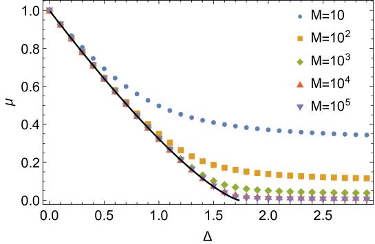
Figure 6: $\Delta$ dependence of the Lagrange multiplier $\mu$ of the continuous distribution for $n=2$ and for several $M$. Markers denote results for finite $M$, while the solid line denotes the result for $M\to\infty$.

In Fig. 7, we plot $q_{1}$ and $q_{1}/M$ for several $M$. For $\Delta\leq\Delta_{c}$, $q_{1}$ converges to $1/\mu_{\infty}^{2}$ in the limit $M\to\infty$, see Fig. 7 (a). On the contrary, for $\Delta>\Delta_{c}$, $q_{1}/M$ converges to Eq. (63), see Fig. 7 (b).

Figure 7: $\Delta$ dependence of the overlap of the continuous distribution for $n=2$. Markers denote results for finite $M$, while the solid line denotes the result for $M\to\infty$.

As in Eq. (53), we use a Gaussian approximation to calculate the participation ratio [8]:

$${\rm PR}=\left[\frac{1}{N}\sum_{i=1}^{N}\left\langle x_{i}^{4}\right\rangle\right]^{-1}\approx\left[\frac{1}{N}\sum_{i=1}^{N}3\left\langle x_{i}\right\rangle^{2}\right]^{-1}=\frac{1}{3}\left[\frac{1}{M}\sum_{k=1}^{M}q_{k}^{2}\right]^{-1}.$$ (64)

For $\Delta\leq\Delta_{c}$, the summation is expressed by an integral, and we get

$${\rm PR}=\frac{1}{3}\frac{1}{\int_{-\infty}^{\infty}dhP(h)q(h)^{2}}.$$ (65)

At the transition point, the denominate is evaluated as

$$\int dhP(h)q(h)^{2}\to\frac{(1+n)}{\Delta^{n+1}}\int_{0}^{\Delta}h^{n-4}dh=\begin{cases}\infty&n\leq 3\\ \frac{n+1}{n-3}\frac{1}{\Delta^{2}}&n>3\end{cases}$$ (66)

Therefore, at the transition point, Eq (65) vanishes for $n\in(1,3]$ and has a finite value for $n>3$. On the contrary, for $\Delta>\Delta_{c}$, the condensation $q_{1}=O(M)$ leads to ${\rm PR}\to 0$ in the limit $M\to\infty$. Those arguments suggest that on approaching the transition point, ${\rm PR}$ continuously goes to zero for $n\in(1,3]$, while it changes discontinuously from a finite value to zero for $n>3$. In Fig. 8, we plot ${\rm PR}$ for finite $M$ calculated by Eq. (64) and for $M\to\infty$ calculated by Eq. (65) for $n=2$. One can see that${\rm PR}$ changes continuously at $\Delta_{c}$, in contrast with the binary distribution where ${\rm PR}$ changes discontinuously at the transition point, see Fig. 4.

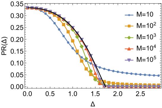
Figure 8: $\Delta$ dependence of the participation ratio ${\rm PR}$ of the continuous distribution for $n=2$. Markers denote the results for finite $M$, while the solid line denotes the result for $M\to\infty$.

Finally, In Figs. 9, 10, and 11, we compare the theoretical prediction and numerical results obtained by direct diagonalization of $W$ for $M=10$ and $100$. We fond good agreement for $M=10$, while there are small but visible finite size effects for $M=100$. This is a natural result because our theory requires $N\gg M$. So we expect larger finite size effects for larger $M$.

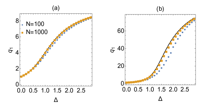
Figure 9: $\Delta$ dependence of $q_{1}$ for $n=2$. Markers denote numerical results, while the solid line denotes the theoretical prediction. (a) Results for $M=10$. (b) Results for $M=100$.

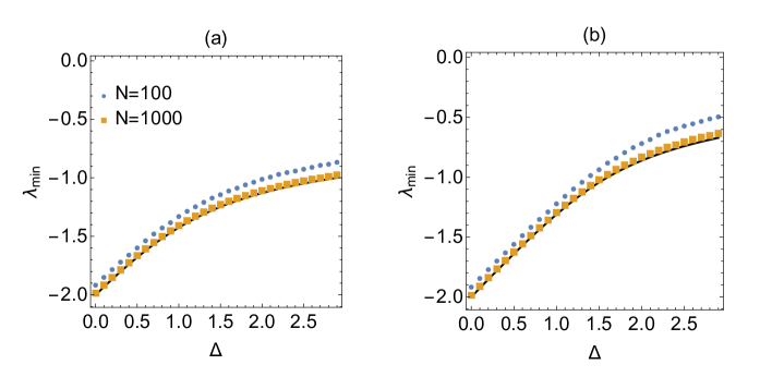
Figure 10: $\Delta$ dependence of $\lambda_{\rm min}$ for $n=2$. Markers denote numerical results, while the solid line denotes the theoretical prediction. (a) Results for $M=10$. (b) Results for $M=100$.

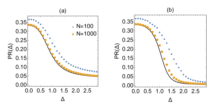
Figure 11: $\Delta$ dependence of ${\rm PR}$ for $n=2$. Markers denote numerical results, while the solid line denotes the theoretical prediction. (a) Results for $M=10$. (b) Results for $M=100$.

5 Summary and discussions

In this work, we investigated the eigenvector $\bm{x}_{\rm min}$ of the minimal eigenvalue $\lambda_{\rm min}$ of a deformed random matrix, where the $i$-th diagonal element of the Wigner matrix is perturbed by a constant $h_{i}$. By using the replica method, we closely analyzed the localization phenomena of $\bm{x}_{\rm min}$ in two cases: when $h_{i}$ has a binary distribution, and when it has a continuous distribution.

For the binary distribution of $h_{i},$ we considered the following distribution function: $P(h)=c\delta(h)+(1-c)\delta(h-\Delta)$, where $c\in[0,1]$ denotes the fraction of non-perturbed sites, and $\Delta>0$ denotes the strength of the perturbation. On increasing $\Delta$, $\bm{x}_{\rm min}$ tends to condensate to the non-perturbed sites. For $c>0$, this condensation is a crossover: the order parameter just gradually increases on increasing $\Delta$. As $c$ decreases, the crossover becomes sharper and eventually becomes a phase transition in the limit $c\to 0$. At the transition point, the condensation to the non-perturbed spins leads to a strong localization. As a consequence, the participation ratio changes discontinuously from a finite value to zero. In the case of a continuous distribution, we considered a power-law distribution $P(h)\propto h^{n}$. We fond that when $n>1$, $\bm{x}_{\rm min}$ exhibits the Bose-Einstein (like) condensation transition, as previously fond for a fully-connected vector spin-glass [8]. At transition point, $\bm{x}_{\rm min}$ tends to condensate to the non-perturbed sites as in the case of the binary distribution, but this time the participation ratio goes to zero continuously for $n\in(1,3]$, and discontinuously for $n>3$.

There are still several important points that deserve further investigation. Here we give a tentative list:

• We speculate that the condition $n>1$ for the existence of the localized phase is somehow universal. Recently, Shimada et al. investigated the localization transition of a $d$-dimensional disordered lattice by using the effective medium theory [37, 38, 39]. They found that for the localized mode to exist, the distribution of the stiffness $k$ should be $P(k)\sim k^{n}$ with $n>1$ for $k\ll 1$. Interestingly, this condition is very similar to that we observed in the case of a continuous distribution of $h_{i}$. Furthermore, a phenomenological theory also supports $n>1$ [40]. Further theoretical and numerical studies would be beneficial to clarify this point [36].

• The interaction potential of our model Eq. (4) is the same of that of the $p=2$-spin spherical model with site disorders [18]. In this work, we only investigate the model at zero temperature. It would be interesting to see how the model behaves at finite temperatures, which may give some insights for the thermal excitation of the localized models of amorphous solids [41, 42].

• It is known that for $p>2$, the $p$-spin spherical model exhibits the one-step replica symmetric breaking (1RSB) [18]. Investigating how the 1RSB transition competes with the condensation transition may provide useful insight into the competition between glass transition and real-space condensation [43], such as gelation [44, 45].

• Important future work is to perform a similar calculation for the Wishart matrix, which has been used to describe the vibrational density of states of amorphous solids near the jamming transition point [19]. A recent numerical simulation revealed that the participation ratio of the lowest localized mode diverges on approaching the jamming transition point, which characterizes the correlated volume near the transition point [46]. It may be possible to derive these behaviors analytically by analyzing a deformed Wishart matrix.

• We expect that our method to treat the site randomness can be applied to other disordered models. A promising candidate would be the random replicant model (RRM), which is a toy model of the coevolution of species [47, 48]. The interaction potential of the RRM is written as

  $$H=\sum_{ij}J_{ij}x_{i}x_{j}+a\sum_{i=1}^{N}x_{i}^{2},$$ (67)

  where $x_{i}$ denotes the number of the species. The interaction is very similar to that of the $p=2$-spin spherical model Eq. (4), but $x_{i}$ should be positive and satisfy the following condition $\sum_{i=1}^{N}x_{i}=N$. It is interesting to see whether condensation transitions occur when the site randomness $\sum_{i}h_{i}x_{i}^{2}$ is added to the RRM, and if so, to investigate the implications of the transition for coevolution.

Appendix A Binary distribution in the limit $c\to 0$ and Baik-Ben Arous-Péché (BBP) transition

Here we briefly discuss that the transition in the $c\to 0$ limit of the binary distribution can be identified with the Baik-Ben Arous-Péché (BBP) transition. A typical setting of the BBP transition is to add a rank-one perturbation to the Wishart matrix $J$:

$$J+\Delta\bm{e}_{i}\bm{e}_{i}^{t},$$ (68)

where $\bm{e}_{i}$ denotes the unit vector along the $i$-th axis. Since the qualitative results do not depend on $i$, we will set $i=1$ in the following. The maximal eigenvalue of the above matrix has been studied extensively, and it is known that in the thermodynamic limit $N\to\infty$ [49]

$$\lambda_{\rm max}=\begin{cases}2&\Delta\leq 1\\ \Delta+1/\Delta&\Delta>1.\end{cases}$$ (69)

The maximal eigenvalue $\lambda_{\rm max}$ exhibits a singular behavior at the critical point $\Delta_{c}=1$, which is the signature of the BBP transition [49].

Now we dicuss that the BBP transition can be identified with the transition of our model with the binary distribution in the limit $c\to 0$. The matrix $W$ with the binary distribution can be written explicitly as follows:

$$W=J+\Delta I-\Delta\sum_{i=1}^{cN}\bm{e}_{i}\bm{e}_{i}^{t},$$ (70)

where $\bm{e}_{i}$ denotes the unit vector along the $i$-th axis, and $I$ denotes the $N\times N$ identity matrix. The minimal eigenvalue is expressed as

$$\lambda_{\rm min}(c) =\min_{\bm{e}}\bm{e}^{t}W\bm{e}=-\lambda_{\rm max}(c)+\Delta$$ (71)

where $\bm{e}$ denotes an unit vector, and

$$\lambda_{\rm max}(c)=-\min_{\bm{e}}\bm{e}^{t}\left(J-\Delta\sum_{i=1}^{cN}\bm{e}_{i}\bm{e}_{i}^{t}\right)\bm{e}=\max_{\bm{e}}\bm{e}^{t}\left(J^{\prime}+\Delta\sum_{i=1}^{cN}\bm{e}_{i}\bm{e}_{i}^{t}\right)\bm{e},$$

$$J^{\prime}=-J.$$ (72)

Since the distribution of $J_{ij}$ is symmetric, $J^{\prime}$ has the same statistical properties of those of $J$. The question is if $\lambda_{\rm max}(c)$ converges to the result of the rank-one perturbation Eq. (69) in the limit $c\to 0$. The answer is yes: by substituting Eq. (49) into (71), one can easily show that $\lim_{c\to 0}\lambda_{\rm max}(c)=\lambda_{\rm max}$. This means that the singularity of $\lim_{c\to 0}\lambda_{\rm max}(c)$, or equivalently $\lim_{c\to 0}\lambda_{\rm min}(c)$, of our model is the consequence of the BBP transition.

References

References

- [1] Rosenzweig N and Porter C E 1960 Phys. Rev. 120(5) 1698–1714 URL https://link.aps.org/doi/10.1103/PhysRev.120.1698
- [2] Kravtsov V, Khaymovich I, Cuevas E and Amini M 2015 New Journal of Physics 17 122002
- [3] Capitaine M and Donati-Martin C 2016 arXiv preprint arXiv:1607.05560
- [4] Facoetti D, Vivo P and Biroli G 2016 EPL (Europhysics Letters) 115 47003
- [5] Lee J O and Schnelli K 2016 Probability Theory and Related Fields 164 165–241
- [6] Livan G, Novaes M and Vivo P 2018 Monograph Award 63
- [7] Aspelmeier T and Moore M A 2004 Phys. Rev. Lett. 92(7) 077201 URL https://link.aps.org/doi/10.1103/PhysRevLett.92.077201
- [8] Franz S, Nicoletti F, Parisi G and Ricci-Tersenghi F 2022 SciPost Physics 12 016
- [9] Franz S, Nicoletti F and Ricci-Tersenghi F 2022 Journal of Statistical Mechanics: Theory and Experiment 2022 053302
- [10] Perry A, Wein A S, Bandeira A S and Moitra A 2018 The Annals of Statistics 46 2416–2451
- [11] Krajenbrink A, Le Doussal P and O’Connell N 2021 Phys. Rev. E 103(4) 042120 URL https://link.aps.org/doi/10.1103/PhysRevE.103.042120
- [12] Rainone C, Urbani P, Zamponi F, Lerner E and Bouchbinder E 2021 SciPost Physics Core 4 008
- [13] Bouchbinder E, Lerner E, Rainone C, Urbani P and Zamponi F 2021 Physical Review B 103 174202
- [14] Lerner E, Düring G and Bouchbinder E 2016 Phys. Rev. Lett. 117(3) 035501 URL https://link.aps.org/doi/10.1103/PhysRevLett.117.035501
- [15] Mizuno H, Shiba H and Ikeda A 2017 Proceedings of the National Academy of Sciences 114 E9767–E9774
- [16] Angelani L, Paoluzzi M, Parisi G and Ruocco G 2018 Proceedings of the National Academy of Sciences 115 8700–8704
- [17] Wang L, Ninarello A, Guan P, Berthier L, Szamel G and Flenner E 2019 Nature communications 10 1–7
- [18] Castellani T and Cavagna A 2005 Journal of Statistical Mechanics: Theory and Experiment 2005 P05012
- [19] Franz S, Parisi G, Urbani P and Zamponi F 2015 Proceedings of the National Academy of Sciences 112 14539–14544
- [20] Folena G and Urbani P 2022 Journal of Statistical Mechanics: Theory and Experiment 2022 053301
- [21] Mézard M, Parisi G and Virasoro M A 1987 Spin glass theory and beyond: An Introduction to the Replica Method and Its Applications vol 9 (World Scientific Publishing Company)
- [22] Parisi G, Urbani P and Zamponi F 2020 Theory of simple glasses: exact solutions in infinite dimensions (Cambridge University Press)
- [23] Edwards S F and Jones R C 1976 Journal of Physics A: Mathematical and General 9 1595
- [24] Sommers H J, Crisanti A, Sompolinsky H and Stein Y 1988 Phys. Rev. Lett. 60(19) 1895–1898 URL https://link.aps.org/doi/10.1103/PhysRevLett.60.1895
- [25] Rodgers G J and Bray A J 1988 Phys. Rev. B 37(7) 3557–3562 URL https://link.aps.org/doi/10.1103/PhysRevB.37.3557
- [26] Semerjian G and Cugliandolo L F 2002 Journal of Physics A: Mathematical and General 35 4837
- [27] Nagao T and Tanaka T 2007 Journal of Physics A: Mathematical and Theoretical 40 4973
- [28] Kühn R 2008 Journal of Physics A: Mathematical and Theoretical 41 295002
- [29] Urbani P 2022 arXiv preprint arXiv:2203.01899
- [30] Kabashima Y and Takahashi H 2012 Journal of Physics A: Mathematical and Theoretical 45 325001
- [31] Sherrington D and Kirkpatrick S 1975 Phys. Rev. Lett. 35(26) 1792–1796 URL https://link.aps.org/doi/10.1103/PhysRevLett.35.1792
- [32] Nieuwenhuizen T M 1995 Phys. Rev. Lett. 74(21) 4289–4292 URL https://link.aps.org/doi/10.1103/PhysRevLett.74.4289
- [33] Cugliandolo L F and Dean D S 1995 Journal of Physics A: Mathematical and General 28 4213
- [34] Fyodorov Y V, Perret A and Schehr G 2015 Journal of Statistical Mechanics: Theory and Experiment 2015 P11017
- [35] Franz S, Parisi G, Sevelev M, Urbani P and Zamponi F 2017 SciPost Phys. 2(3) 019
- [36] Stanifer E, Morse P, Middleton A and Manning M 2018 Physical Review E 98 042908
- [37] Shimada M, Mizuno H and Ikeda A 2020 Soft Matter 16 7279–7288
- [38] Shimada M, Mizuno H and Ikeda A 2021 Soft Matter 17 346–364
- [39] Shimada M and De Giuli E 2022 SciPost Physics 12 090
- [40] Gurarie V and Chalker J T 2003 Phys. Rev. B 68(13) 134207 URL https://link.aps.org/doi/10.1103/PhysRevB.68.134207
- [41] Das P and Procaccia I 2021 Phys. Rev. Lett. 126(8) 085502 URL https://link.aps.org/doi/10.1103/PhysRevLett.126.085502
- [42] Guerra R, Bonfanti S, Procaccia I and Zapperi S 2022 Phys. Rev. E 105(5) 054104 URL https://link.aps.org/doi/10.1103/PhysRevE.105.054104
- [43] Majumdar S 2010 Exact Methods in Low-dimensional Statistical Physics and Quantum Computing: Lecture Notes of the Les Houches Summer School: Volume 89, July 2008 407
- [44] Zaccarelli E, Buldyrev S V, La Nave E, Moreno A J, Saika-Voivod I, Sciortino F and Tartaglia P 2005 Phys. Rev. Lett. 94(21) 218301 URL https://link.aps.org/doi/10.1103/PhysRevLett.94.218301
- [45] Manley S, Wyss H M, Miyazaki K, Conrad J C, Trappe V, Kaufman L J, Reichman D R and Weitz D A 2005 Phys. Rev. Lett. 95(23) 238302 URL https://link.aps.org/doi/10.1103/PhysRevLett.95.238302
- [46] Shimada M, Mizuno H, Wyart M and Ikeda A 2018 Phys. Rev. E 98(6) 060901 URL https://link.aps.org/doi/10.1103/PhysRevE.98.060901
- [47] Diederich S and Opper M 1989 Physical Review A 39 4333
- [48] Biscari P and Parisi G 1995 Journal of Physics A: Mathematical and General 28 4697
- [49] Potters M and Bouchaud J P 2020 A First Course in Random Matrix Theory: For Physicists, Engineers and Data Scientists (Cambridge University Press)