Searching for cataclysmic variable stars in unidentified X-ray sources

Abstract

We carry out a photometric search for new cataclysmic variable stars (CVs), with the goal of identification for candidates of AR Scorpii-type binary systems. We select GAIA sources that are likely associated with unidentified X-ray sources, and analyze the light curves taken by the Zwicky Transient Facility, Transiting Exoplanet Survey Satellite, and Lulin One-meter Telescope in Taiwan. We investigate eight sources as candidates for CVs, among which six sources are new identifications. Another two sources have been recognized as CVs in previous studies, but no detailed investigations have been done. We identify two eclipsing systems that are associated with an unidentified XMM-Newton or Swift source, and one promising candidate for polar associated with an unidentified ASKA source. Two polar candidates may locate in the so-called period gap of a CV, and the other six candidates have an orbital period shorter than that of the period gap. Although we do not identify a promising candidate for AR Scorpii-type binary systems, our study suggests that CV systems that have X-ray emission and do not show frequent outbursts may have been missed in previous surveys.

1 Introduction

The cataclysmic variable star (hereafter CV) is a binary system composed of a white dwarf primary (hereafter WD) and a low-mass main-sequence star (Warner, 1995). In the usual CV system, the mass is transferred from the companion star to the WD, and it forms an accretion disk extending down to the WD surface or accretion column on the WD’s pole, toward which the accreting matter is channeled by the WD’s magnetic field. The former and latter systems usually belong to nonmagnetic and magnetic CV systems, respectively. A nonmagnetic CV shows frequent outbursts due to an instability of the accretion disk (dwarf nova). Magnetic CVs, in which the WD’s magnetic field is $B_{WD}>10^{5}$ G, are divided into two types, namely, intermediate polar (hereafter IP) and polar. In an IP system, the spin period of the WD is different from the orbital period of the system. Polar has the strongest magnetic field and shows a spin-orbit phase synchronization. CVs are usually observed in the optical to X-ray bands, for which emission originates from the boundary layer of the accretion disk, the companion star surface, or the WD surface/accretion column.

Numerous efforts to identify new CVs and candidates have been made in previous works, and the number of known CVs is rapidly increasing with recent photometric and spectroscopic all-sky surveys (Ritter & Kolb, 1998; Coppejans et al., 2016; Sun et al., 2021; Szkody et al., 2021). The methods of confirming CVs are mainly divided into three types, namely, the observation of dwarf-nova outbursts, identification of orbital/WD spin variations in photometric light curves, and confirmation of CV-like spectral properties. The Open Cataclysmic Variable Catalog (Jackim et al., 2020) offers a vast list of the known CVs and the CV candidates found in previous studies.

Among known WD binary systems, AR Scorpii is one of the special classes in terms of the observed emission properties. The emission in the radio to X-ray bands is modulating with a spin period of WD ($\sim 117$ s) and/or a beat period ($\sim 118$ s) between the WD spin and orbital motion, and its broadband spectrum is described by a nonthermal emission process plus thermal emission from the companion star surface (Marsh et al., 2016; Buckley et al., 2017; Stanway et al., 2018; Takata et al., 2018). Although there has not yet been a direct measurement of the magnetic field of a WD (Garnavich et al., 2021a), the observational properties suggest a magnetic WD binary system. The emission in the optical and X-ray bands is also modulating with the orbital period of $\sim 3.56$ hr, and the shape of the orbital light curve suggests heating of the dayside of the companion star at a rate of $L_{irr}\sim 10^{32-33}~{}{\rm erg~{}s^{-1}}$, most of which is converted into emission in the IR/optical/UV bands. The multiwavelength spectrum exhibits no features of emission from an accretion disk in the system, and the emission from the WD is fainter than the observed optical emission, which cannot be the source of the heating of the companion star. It is therefore suggested that the magnetic field of the WD may be the energy source of the heating, and it is interacting with the companion star or outflow matter from the companion (Takata et al., 2017; Katz, 2017; Lyutikov et al., 2020). AR Scorpii may be classified as an IP in the sense that the spin period of the magnetic WD is shorter than the orbital period. However, the X-ray luminosity is of the order of $L_{X}\sim 4\times 10^{30}~{}{\rm erg~{}s^{-1}}$, which is two to three orders of magnitude lower than that of typical IPs, in which the X-ray emission originated from the accretion column on the WD. Attention has been paid to AR Scorpii to study the origin of the magnetic field of the WD (Schreiber et al., 2021; Wilson et al., 2021).

An AR Scorpii-type binary system will be a new astrophysical laboratory for nonthermal processes, and it may be the origin of cosmic-ray electrons. A second AR Scorpii, however, has not yet been identified, and the population in the galaxy has not been understood. AE Aquarii/LAMOST J024048.51+195226.9 (Pelisoli et al., 2022) are known as a magnetic WD system in the propeller phase, and they are similar to AR Scorpii in the sense that (i) no accretion disk is formed and (ii) the system contains a fast-spinning WD (Patterson, 1979; Wynn et al., 1997; Pretorius et al., 2021; Garnavich et al., 2021b). On the other hand, there is no evidence of heating of the companion star, and the existence of the nonthermal emission extending in broad energy bands (radio to X-ray/gamma-ray bands) has not been established; for AE Aquarii, although evidence of the nonthermal emission in X-ray and TeV energy bands has been reported (Meintjes et al., 1994; Terada et al., 2008), the results have not been confirmed by follow-up observations (Kitaguchi et al., 2014; Aleksić et al., 2014; Li et al., 2016). CTCV J2056-3014 and V1460 Her also contain fast-spinning WD, and they are classified as X-ray faint IPs (Lopes de Oliveira et al., 2020; Ashley et al., 2020). Spectroscopic studies suggest that CTCV J2056-3014 and V1460 Her contain accretion disks and hence their WDs will have a weak magnetic field.

AR Scorpii has faint X-ray emission and has not shown a dwarf-nova-type outburst. Moreover, AR Scorpii contains a WD with a relatively cool surface temperature, and does not show a deep eclipsing feature in the light curve. Binary systems with such featureless emission properties may have at first glance, been missed by previous surveys, and may require a different approach to confirm new AR Scorpii-type binary systems. In this study, we take the approach of finding new CVs in unidentified X-ray sources, since the X-ray emission as a result of the interaction between the WD’s magnetic field and the companion star is a unique property of AR Scorpii. The structure of this paper is as follows. Section 2 describes our strategy and method for searching for new CV candidates. Section 3 presents eight candidates including six new identifications and two sources that have been recognized as CV candidates but have not been listed in the current catalogs. Although our new candidates will not be categorized as a new AR Scorpii-type binary system, searching in the unidentified X-ray sources offers an alternative approach to identifying new CV systems. In section 4, we compare the UV and X-ray emission properties of our candidates with those of known CVs.

2 Searching method

2.1 candidate selection

First, we select candidates of the WD/low-mass main-sequence star binary systems from the GAIA DR2 source list (Gaia Collaboration et al., 2018). In the GAIA color-magnitude diagram, AR Scorpii, CTCV J2056-3014 and the typical CV systems are located between the main-sequence and the cooling sequence of the WD (Figure 1). In this work, therefore, we limit the range of the search with a color of $0.5<G_{BP}-G_{RP}<1.5$ ($G_{BP}$ and $G_{RP}$ are blue and red magnitude defined by the GAIA photometric system, respectively) and a magnitude of $9<M_{G}<12$. We do not limit the range of the parallax, but restrict the magnitude of the error with a cut parallax_over_error > 5 in the query. To obtain a clean sample, we refer to Lindegren et al. (2018) and apply the conditions that

• phot_bp_mean_flux_over_error > 8

• phot_rp_mean_flux_over_error > 10

• astrometric_excess_noise < 1

• phot_bp_rp_excess_factor < 2.0+0.06* power(phot_bp_mean_mag-phot_rp_mean_mag,2)

• phot_bp_rp_excess_factor > 1.0+0.015* power(phot_bp_mean_mag-phot_rp_mean_mag,2)

• visibility_periods_used > 5.

We downloaded a catalog of the GAIA sources using astroquery (Ginsburg et al., 2019).

We search for a possible X-ray counterpart of the selected GAIA sources in (i) the ROSAT all-sky survey bright source catalog (Voges et al., 1999), (ii) the second Swift-XRT point-source catalog (Evans et al., 2020) and (iii) XMM-Newton DR-10 source catalog (Webb et al., 2020). We select the GAIA sources that are located within 10” from the center of the X-ray source, and then we remove the sources that have been already identified as a CV or other types of objects by checking the catalogs of CVs (Ritter & Kolb, 2003; Coppejans et al., 2016; Jackim et al., 2020; Sun et al., 2021; Szkody et al., 2021), and the SIMBAD astronomical database.

After selecting the GAIA sources that are potentially associated with unidentified X-ray sources, we cross match them with sources observed by the Zwicky Transient Facility DR-8 objects (hereafter ZTF, Masci et al., 2019). We select a potential candidate of CVs based on (i) identification of a signature of an outburst and (ii) a periodic search with a Lomb-Scargle periodogram (hereafter LS, Lomb, 1976). We download the light curves from the Infrared Science Archive , and use the $r$-band data to search for a periodic signal. We apply the barycentric correction to the photon arrival time using astropy. We find, on the other hand, that since the ZTF observation for our candidates (section 3) provides only $500-1000$ data points during 2018-2021 observations, the data quality may not be enough to study the detailed properties of the light curve (e.g. identifying eclipse feature, section 3.1).

The Transiting Exoplanet Survey Satellite (hereafter TESS, Ricker et al., 2014) provide the light curves of the sources by monitoring for a month, and also photometric data of sources that are out of the field of view of ZTF. For our targets, TESS full-frame images (hereafter FFIs) provides the data taken every 10 minutes or 30 minutes, for which Nyquist frequencies are $F_{N}\sim 72~{}{\rm day^{-1}}$ and $\sim 24~{}{\rm day^{-1}}$, respectively. We extract the light curve of the pixels around the source region from TESS-FFIs using TESS analysis tools, eleanor (Feinstein et al., 2019; Brasseur et al., 2019) and Lightkurve (Lightkurve Collaboration et al., 2018). We note that since several GAIA sources are usually located at one pixel, TESS data alone cannot tell us which source produces the periodic signal in a light curve extracted from TESS-FFIs. To complement ZTF and TESS observations, we carry out photometric observations for some of our targets with the Lulin One-meter Telescope (hereafter LOT) in Taiwan.

2.2 LS periodogram

First, we produce an LS periodogram for each source by taking into account the Gaussian and uncorrelated errors that are usually provided in the archival data (or by usual data processing). We search for a possible periodic signal in $1~{}{\rm day^{-1}}<f<50-150~{}{\rm day^{-1}}$, in which the maximum frequency depends on the time resolution of the observation. We estimate the false alarm probability (hereafter FAP) of the signal with the methods of Baluev (2008) and of the bootstrap (VanderPlas, 2018). For an accreting system, it is proposed to investigate the effect of the time-correlated noise on the LS periodogram (VanderPlas, 2018). Based on the correlated noise model of Delisle et al. (2020), we, therefore, produce an LS periodogram with different parameters of the noise model (Appendix A). We find that the LS periodogram of TESS data is insensitive to time-correlated noise model. For ZTF data, although the noise model can change the shape of the LS periodogram, it is less effective in the periodic signals presented in this study (Table 1); but see section 3.1 and Appendix A for ZTF18aampffv, in which one periodic signal may be related to time-correlated noise. In section 3, therefore, we present an LS periodogram created with the time uncorrelated noise. The correlated noise model and some results of the LS periodogram are presented in Appendix A.

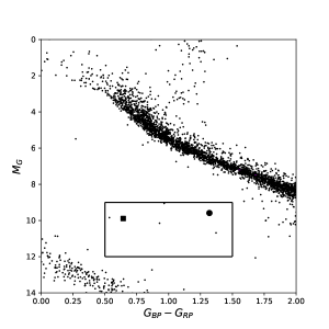
Figure 1: Color-magnitude diagram of GAIA sources. The square represents the search region in our study. The filled circle and box correspond to AR Scorpii and CTCV J2056-3014, respectively.

3 Results

Table 1: Basic information on the CV candidates in this study

GAIA	ZTF	X-ray source	Distance	$f_{ZTF}/F_{0}$	Orbital	Proposed type
DR2			(pc)	(${\rm day^{-1}}$)	frequency
1415247906500831744 (G141)	18aampffv	4XMM J172959.0+52294	532	- /11.148(4)	$F_{0}$	Eclipsing
4534129393091539712 (G453)	18abikbmj	1RXS J185013.9+242222	322	- / 39.11(4)	$F_{0}$/2 or $F_{0}$	Dwarf-Nova/superhump
2072080137010352768 (G207)	18abrxtii	2SXPS J195230.9+372016	313	28.575(1)/28.57(4)	$F_{0}$/2	Eclipsing
2056003803844470528 (G205)	18aayefwp	2SXPS J202600.8+333940	595	24.595(1)/24.60(4)	$F_{0}$/2 or $F_{0}$
2162478993740496256 (G216)	17aaapwae	2SXPS J211129.4+445923	429	22.175(1)/22.18(2)	$F_{0}$
4321588332240659584 (G432)	18aazmehw	2SXPS J192530.4+155424	582	18.5521(9)/18.553(1)	$F_{0}$/2 or $F_{0}$	IP
4542123181914763648 (G454)	18abttrrr	1RXS J172728.8+132601	502	8.6499(8)/8.65(2)	$F_{0}$	Polar

Table 2: Information on TESS and LOT observations

GAIA	TESS		LOT		Figures
DR2	Date (MJD)	Sector	Date (MJD)	Exposure (hrs)
G141	58764-58789	17	59491/59492	5.2	2-5, A1
	58954-59034	24, 25, 26
	59579-59606	47
	59664-59690	50
G453	59009-59034	26	59398/59399	4.9	6-9
G207	58683-58736	14, 15	59475/59476	2.8	10,11
	59419-59445	41
G205	58683-58736	14, 15	59542	0.7	10, A1
	59419-59445	41
G216	58710-58762	15, 16	59474	2.7	10,12
G432	58682-58709	14			13,14
	59390-59418	40
G454	58984-59034	25, 26			15

Table 3: Summary of Swift X-ray observations

GAIA	Data	Date/Exposure	$N_{H}$	Photon index	Luminosity
DR2		(MJD)/(ks)	$10^{22}(\rm{cm^{2}})$		$10^{31}({\rm erg~{}s^{-1}})$
G141	TOO	59558/4.7	$1.9^{+5.4}_{-1.9}$	$0.5^{+0.6}_{-0.5}$	$4.5^{+1.9}_{-1.3}$
G453	TOO	59529, 59534/2.0	$1.4^{+2.5}_{-1.4}$	$1.6^{+0.7}_{-0.6}$	$5.5^{+2.0}_{-1.5}$
G207	Archive	57046, 57047/3.2	0.3 (fixed)	$0.9^{+1.0}_{-1.0}$	$0.5^{+0.8}_{-0.3}$
G205	Archive	57796-57806/9.1	$4.0^{+5.2}_{-2.0}$	$2.4^{+1.1}_{-0.9}$	$1.4^{+3.4}_{-0.6}$
G216	Archive	57210-57309/10	4.0 (fixed)	$1.8^{+0.4}_{-0.4}$	$1.2^{+0.4}_{-0.3}$
G432	Archive	56011-56074/1.1	13 (fixed)	$0.3^{+1.1}_{-1.4}$	$14^{+24}_{-8.0}$
G454	TOO	59591/2.5	0.75 (fixed)	$-0.2^{+1.0}_{-1.6}$	$5.5^{+14}_{-3.2}$

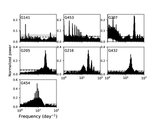
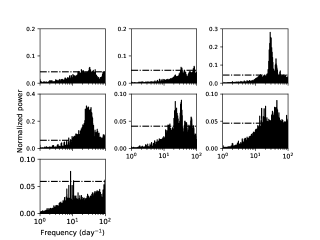
Figure 21: Left : The LS-periodograms of ZTF data for the seven candidates listed in Table 1 with Gaussian and time uncorrelated noise model [the first term in Equation of (20)]. The dashed and dotted lines are FAP=0.01 estimated by the methods of Baluev (2008) and of the bootstrap, respectively. Right : The LS-periodograms with time correlated noise model [the full expression of (20)]. The results are for $\tau_{exp}=1$ day, and $\sigma_{exp}=1$ mag, (for G131, G207, G205 and G216) or 0.5 magnitude (for G453, G432 and G454). The dashed-dotted line represents FAP=0.01 estimated from the method of Delisle et al. (2020).

We downloaded the catalog of $\sim 2\times 10^{5}$ GAIA sources selected based on criteria described in section 2, and identify 29 sources that are potential counterparts of the unidentified X-ray sources. After searching for period signals in the light curves based on ZTF, TESS, and LOT data, we identify seven sources as being CV candidates (Tables 1-3, sections 3.1-3.5), for which we can obtain a periodic signal with at least two different facilities. Two of them have been recognized as candidates for CVs in previous studies, but they are not listed in the current catalogs. We also present four other sources (Table 4, section 3.6), for which no useful ZTF data are available, but TESS-FFI data indicates a periodic signal, and one of them is a promising candidate for polar. LS periodograms and light curves obtained from ZTF and TESS data for 11 candidates are presented in Figures 21-24.

3.1 GAIA DR2 1415247906500831744

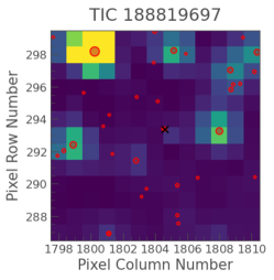
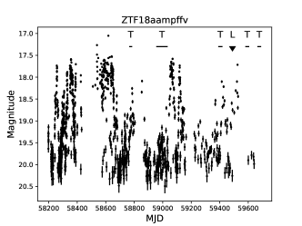
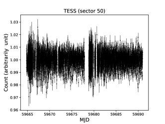
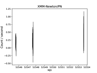
Figure 2: Top left: TESS-FFI image of G141. The cross symbol and red circles indicate the position of the target and the GAIA sources with a magnitude $m>20$, respectively. Top right : ZTF light curve (g-band) of the target (ZTF18aampffv). ”T”(horizontal bars) and “L” (triangle) indicate the epochs of TESS and LOT observations, respectively. Bottom left : Light curves taken by TESS (sector 50). The light curve extracted from TESS-FFI is corrected with TESS analysis tool Lightcurve(Lightkurve Collaboration et al., 2018). Bottom right: Light curve with XMM-Newton PN data.

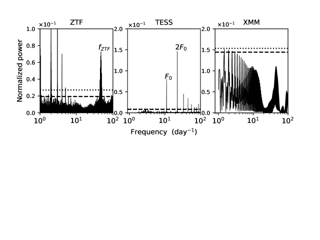
Figure 3: LS periodiagrams of ZTF (left), TESS (middle, sector 50) and XMM-Newton PN (right) data for G141. The dotted and dashed horizontal lines represent the FAP=0.01 estimated by the methods of Baluev (2008) and of the bootstrap (Baluev, 2008). In the TESS data (middle panel), $F_{0}$ represents the orbital period of this system.

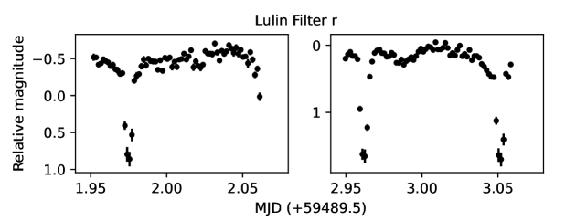
Figure 4: Light curve of G141 taken by LOT. The observation covers three eclipses and confirms an orbital frequency of $F_{0}\sim 11.148~{}{\rm day^{{-1}}}$. In the left panel, the secondary eclipse with a smaller dip can be seen at MJD 2.025+59489.5.

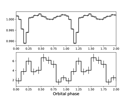
Figure 5: Orbital light curve of G141 measured by TESS (top) and XMM-Newton/PN (bottom). In the TESS light curve, two eclipses can be clearly seen. The data is folded with $F_{0}=11.148~{}{\rm day^{-1}}$ ($\sim 0.090$ day), and phase zero corresponds to MJD 59398.713391.

4XMM J172959.0+522948 (hereafter, 4XMMJ1729) is an unidentified X-ray source, and its position is consistent with GAIA DR2 1415247906500831744 (hereafter G141, Figure 2). Based on the parallax measured by GAIA, the distance to this source is $\sim 532$ pc. There is a nearby source (GAIA DR2 1415247906499736448), whose position from our target is separated by $\sim 2^{\prime\prime}$. Since the GAIA G-band mean magnitude of the nearby source, $\sim 20$, is larger than G141 ($\sim 18.3$ mag), contamination will have less influence on the optical light curve observed for our target.

Figure 2 (top right panel) shows the $r$-band light curve for G141 measured by ZTF (ZTF18aampffv). We find in the figure that the target frequently repeats small outbursts or transitions between high and low states on a timesale of months, which may indicate an accreting system. The amplitude is $\delta m>2$, which is relatively large compared to those seen in the ZTF light curves for other candidates presented in this study. We search for a potential periodic signal in the ZTF light curve with the LS periodogram (left panel of Figure 3), and find a significant signal at $f_{ZTF}\sim 46.9991(9)~{}{\rm day^{-1}}$ ($\sim 0.021$ days), where the uncertainty denotes the Fourier resolution of the observation (namely, the inverse of the time span covered by the observation).

The TESS observation covered the source region several times (Table 2). The middle panel of Figure 3 shows an LS periodogram of the light curve of the TESS data, the sector 50 (Figure 2). The time resolution of the sector 50 is about 10 minutes, and it has the capability to searching for a signal of $f_{ZTF}\sim 47~{}{\rm day^{-1}}$. We find, however, that the LS periodogram is dominated by the signal with $\sim 22~{}{\rm day^{-1}}$, which is indicated with $2F_{0}$ in the figure, its harmonics and aliasing signals. We check the data of sector 47, which also does not show a significant periodic signal at $f_{ZTF}$. Since the data of sectors 17 and 24-26 were taken approximately every $30$ minutes, they cannot be used to search for a periodic signal of $f_{ZTF}$. The signal of $\sim 22~{}{\rm day^{-1}}$ is confirmed in all data (although sector 40 also covers the source, the data is contaminated by unusually high background emission or noise).

To collect evidence of a binary nature, we carried out a photometric observation with LOT (2021, October 4th and 5th, Table 2). The light curve clearly shows that G141 is an eclipsing binary system (Figure 4), and the observation covered three eclipse events that repeat at a frequency of $F_{0}=11\pm 4~{}{\rm day^{-1}}$, suggesting that G141 is a binary system with an orbital period of $P_{orb}\sim 0.09$ day. With the time resolution of $\sim$2 minutes for the LOT data, we estimate that each eclipse lasts $\sim 15$ minutes, and the eclipse profile does not change during the observation. With the LOT data, we unable to confirm a periodic signal corresponding to $f_{ZTF}\sim 47~{}{\rm day^{-1}}$.

The top panel of Figure 5 shows the folded light curve of the TESS data with a frequency of $F_{0}\sim 11~{}{\rm day^{-1}}$, and clearly shows an eclipsing feature at the orbital phase of $\sim 0.2$ in the light curve. We also find the secondary eclipse around the orbital phase $\sim 0.7$, which is shallower than that of the primary eclipse. This illustrates that the signal of the second harmonic ($F_{1}=2F_{0}\sim 22.296~{}{\rm day^{-1}}$) is stronger than that of the fundamental signal in the LS periodogram.

4XMMJ1729 was covered by the field of view, when XMM-Newton observations were carried out for two stars (HD 150798 and HD 159181) in 2002. We extract the data in the standard way using the most updated instrumental calibration, tasks emproc for MOS and epproc for PN of the XMM-Newton Science Analysis Software (XMMSAS, version 19.0.1). Although the observation was carried out with a total exposure of about 20 ks, the quality of the data is insufficient to measure the spectral properties, since (i) the target is located at the edge of the field of view in all EPIC data and (ii) the observation is significantly affected by background flare-like events. We create an LS periodogram for the light curve (Figure 2) of PN data; we do not analyze MOS data due to an insufficient count rate. As can be seen in Figure 3, the window effect dominates the periodogram, and a significant periodic signal at $f_{ZTF}\sim 47~{}{\rm day^{-1}}$ is not identified, although an indication may exist. Figure 5 shows the X-ray light curve folded with the orbital period $F_{0}=11.148~{}{\rm day^{-1}}$. Although a lower count rate is observed at $\sim 0\sim 0.3$ orbital phase, a deeper observation is required to investigate the eclipse feature in X-ray bands.

We obtain an $\sim 5$ ks Swift observation for 4XMMJ1729 (Table 3). We extract a cleaned event file with Xselect under HEASoft ver.6-29, and fit the spectrum with Xspec ver.12.12. Since we could not constrain the spectral model because of insufficient photon counts, we fit the spectrum with a single power-law function (Table 3). Using the distance measured by GAIA (Table 1), we estimate the luminosity in the 0.3-10 keV band as $L_{X}=4.5^{+1.9}_{-1.3}\times 10^{31}(d/{\rm 532~{}pc})^{2}~{}\rm{erg~{}s^{-1}}$ (hydrogen column density of $N_{H}=1.9^{+5.4}_{-1.9}\times 10^{21}~{}{\rm cm^{-2}}$ and photon index of $\Gamma=0.5^{+0.6}_{-0.5}$).

We have not found a significant periodic signal with $f_{ZTF}\sim 47~{}{\rm day^{-1}}$ in TESS, LOT and XMM-Newton data. In Appendix A, therefore, we carry out a further investigation of the LS periodogram of the ZTF data and find the possibility that the signal is caused by the time-correlated noise.

3.2 GAIA DR2 4534129393091539712

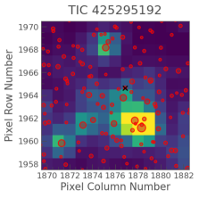
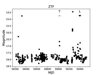
Figure 6: Position (left) and light curve (right) of G453. Left: TESS FFI in the source region overlaid by the GAIA sources (red circles) with a magnitude $m>20$. The center (cross symbol) represents the position of the target. Right: ZTF light curve of the target (ZTF18abikbmj).

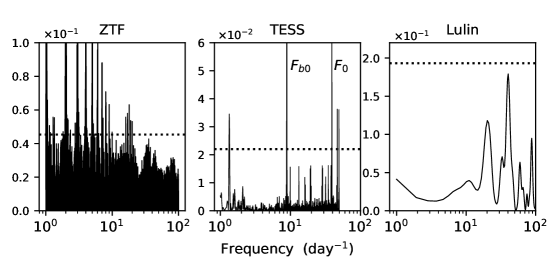
Figure 7: LS periodiagrams of ZTF (left), TESS (middle) and LOT (right) data for G453. The dotted lines show the FAP=0.01 estimated by the bootstrap method.

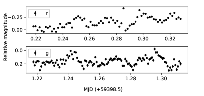
Figure 8: The light curves with the $r$-band (upper) and $g$-band (lower) filters of G453 taken by LOT.

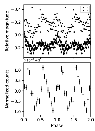
Figure 9: Light curve of G453 folded with $F_{0}/2=19.6~{}{\rm day^{-1}}(\sim 0.05~{}{\rm days})$. Top: Light curves with the $r$-band (circle) and $g$-band (square) taken by LOT. Bottom: Light curve taken by TESS. For TESS data, the counts are binned and each bin covers a 0.1 phase. Phase zero refers to MJD 59398.713391.

GAIA DR2 4534129393091539712 (hereafter, G453) is selected as a possible counterpart of the ROSAT source, 1RXS J185013.9+242222. We obtain an $\sim 2$ ks Swift observation for 1RXS J185013.9+242222 in 2021 November, and we estimate the luminosity of $L_{X}\sim 5.5^{+2.0}_{-1.5}\times 10^{31}(d/322~{}\rm{pc})^{2}~{}{\rm erg~{}s^{-1}}$ in the 0.3-10 keV band by fitting the spectrum with a power-law model ($N_{H}=1.4^{+2.5}_{-1.4}\times 10^{21}~{}{\rm cm^{-2}}$ and $\Gamma=1.6^{+0.7}_{-0.6}$, Table 3).

As can be seen in the right panel of Figure 6, the ZTF light curve (ZTF18abikbmj) shows several outbursts with a recurrent time scale of a year. In fact, 1RXS J185013.9+242222 has already been recognized as a dwarf nova by previous observation of the outburst . Since no detailed investigation for this source has been carried out, we searched for possible orbital modulation in the photometric data.

First, we searched for periodic signals in a quiescent state in the ZTF data, but we did not find any obvious periodic signals (except for the window effects) in the periodogram (Figure 7). TESS observed this source in 2020 June during a stage of the small outburst (Figure 6), and the data was taken approximately every $30$ minutes. We extract the light curve with 4 pixels around the target (left panel of Figure 6). In the LS-periodogram, we find two strong signals at 8.88(4) day^-1 ($\sim 0.11$ days) and 39.11(4) day^-1 ($\sim 0.026$ days), either of which is likely the aliasing of the sampling frequency. Since the extracted light curves with 4 pixels contain several sources (left panel of Figure 7), the TESS observation alone cannot support the detected signal originating from G453.

We confirm the binary nature of G453 with LOT. We carried out the observations with $r$-band (2021 July 3) and g-band (2021 July 4) filters, for which one observation covered the source with an exposure of $\sim 2-2.5$ hr (Table 2). As indicated in Figure 6, the LOT observation was also carried out during a small outburst, which could be a re-brightening after the large outburst happen around MJD 59300. In the LS-periodogram (Figure 7) and the observed light curve (Figure 8), we confirm evidence of periodic modulation at $F_{0}=37.3\pm 1~{}{\rm day^{-1}}$, which is close to the TESS result.

Although we cannot firmly conclude the origin of the periodic signal with the current photometric data, the signal $F_{0}$ is likely related to the orbital period. From the shape of the light curve taken by LOT, we can expect that the orbital period is double the photometric period, namely $P_{orb}\sim 2\times 1/F_{0}\sim 0.05~{}{\rm days}$; e.g. the light curve with the $r$-band filter may be more consistent with modulation caused by the elliptical shape of the companion star that fills the Roche-lobe, and an indication of double-peak structure with the different peak magnitudes in the $g$-bands (Figure 9).

Another possible origin of the signal $F_{0}$ is the superhump, which is a periodic variation observed emission from an eccentric disk after the outburst of CVs (Warner, 1995). The period of the superhump is several percent longer (or sometimes shorter) than the orbital period. Although superhump is usually observed after a super-outburst of CVs (Osaki, 2005; Kato et al., 2014; Hameury, 2020), it has also been observed at normal outburst or re-brightening after a super-outburst (Zhao et al., 2006; Imada et al., 2012). The ZTF light curve of G453 suggests that there were several re-brightenings after the large outburst occurred around MJD 59300, and the LOT observation covered one of re-brightening stages. Moreover, the previous observations for other dwarf novae confirm a beat signal between the orbital modulation and superhump (Patterson et al., 2000; Kato et al., 2010). In the periodogram of the TESS data for G453 (middle panel of Figure 7), we notice a periodic signal at $\sim 1.34~{}{\rm day^{-1}}$ ($\sim 0.75$ day), which is confirmed only at the source region, with a significance greater than the 99 % confidence level. This signal can be explained by the beat signal, if the difference between the orbital period and the superhump period is $\epsilon\sim 3-4$ % (i.e. $1.34~{}{\rm day^{-1}}\sim\epsilon\times 39~{}{\rm day^{-1}}$). The TESS light curve folded with $F_{0}$ is presented in Figure 23.

3.3 GAIA DR2 2072080137010352768, 2056003803844470528, and 2162478993740496256

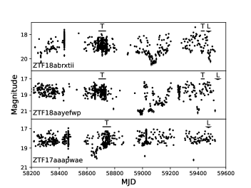
Figure 10: ZTF light curves (the $r$-band filter) for G207 (ZTF 18abrxti), G205(18aayefwp) and G216 (17aaapwae).

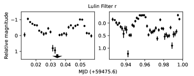
Figure 11: LOT observation (the r-band filter) for G207. The observation covered two eclipses that occurred at MJD 0.034 (+59475.6) indicated by arrow symbol and MJD 0.94 (+59475.6)

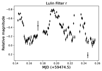
Figure 12: LOT observation (the r-bands filter) for G216.

We find these three candidates that do not show frequent outbursts, but the observed brightness drops suddenly and stays at a low luminosity state with a time scale of months. Figure 10 shows the light curves of GAIA DR2 2072080137010352768 (hereafter G207), 2056003803844470528 (G205), and 2162478993740496256 (G216) measured by ZTF, which are named ZTF 18abrxtii, 18aayefwp, and 17aaapwae, respectively. For G207 (top panel of Figure 10), for example, a sudden drop in brightness occurred around MJD 59050 and the source stayed in a low luminous state for $\sim 50$ day. These three GAIA sources are selected as the optical counterparts of Swift sources. Using the distance measured by GAIA, the X-ray luminosity in the 0.3-10 keV energy band is estimated to be $L_{X}\sim 0.5^{+0.8}_{-0.3}\times 10^{31}(d/313~{}{\rm pc})^{2}~{}{\rm erg~{}s^{-1}}$ for G207, $\sim 1.4^{+3.4}_{-0.6}\times 10^{31}(d/~{}595{\rm pc})^{2}{\rm erg~{}s^{-1}}$ for G205 and $\sim 1.2^{+0.4}_{-0.3}\times 10^{31}(d/429~{}{\rm pc})^{2}{\rm erg~{}s^{-1}}$ for G216, respectively (Table 3).

For these three targets, we can detect significant periodic signals in the ZTF and TESS (Tables 1 and 2). The photometric periodic signals in the ZTF light curves are $f_{ZTF}=28.575(1)~{}{\rm day^{-1}}$ ($\sim 0.035$ day) for G207, $24.595(1)~{}{\rm day^{-1}}$ $(\sim 0.041$ day) for G205 and $22.175(1)~{}{\rm day^{-1}}$ ($\sim 0.045$ day) for G216, respectively. We also obtain consistent periodic signals in the TESS light curves.

We carried out photometric observations for the three sources with LOT. For G207 (Figure 11), although the data fluctuation is significant, we find an eclipsing feature in the light curve. Figure 11 shows that the source became fainter around MJD 0.034 (+59475.6) and MJD 0.094 (+59475.6), and the time interval between two epochs is consistent with an integer multiple of the photometric period of $1/f_{ZTF}\sim 0.035~{}{\rm day}$. The orbital period, however, will be double of the photometric period, since the observation in left panel of Figure 11 should cover another eclipse if the orbital period is $\sim 0.035$ day. ZTF/TESS light curves may indicate a secondary eclipse with a shallower depth (Figure 23).

For G216 (Figure 12), the light curve indicates a periodic modulation, and the time interval between two strong peaks is consistent with the photometric period of $1/f_{ZTF}\sim 0.045$ day, and the LOT light curve is consistent with the TESS/ZTF light curves (Figure 23). Hence, G216 is a binary system with an orbital period of $0.045$ day. For G205, we could carry out only $\sim 40$ minute observation with LOT. The data, therefore, is not enough to constrain the orbital period of the source.

3.4 GAIA DR2 4321588332240659584

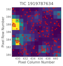
Figure 13: Left: TESS-FFI image around G432, overlaid by the GAIA sources ($m_{g}>20$). The cross at the center of image indicates the position of the target. Right: The light curve of the target measured by ZTF (ZTF18aazmehw).

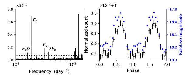
Figure 14: Left; LS-periodogram for light curve of G432 measured by TESS. $F_{0}$ and $2F_{0}$ are frequencies detected in the ZTF light curve and its harmonics, respectively. $F_{u}$ and $F_{u}/2$ are unknown frequencies and its harmonics, respectively. Right: The ZTF (blue) and TESS (black) light curve folded with a frequency of $f_{ZTF}=18.552~{}{\rm day^{-1}}$ ($\sim 0.054$ day). Phase zero corresponds to MJD 59398.713391. The horizontal dotted line shows FAP=0.01 estimated with the bootstrap method.

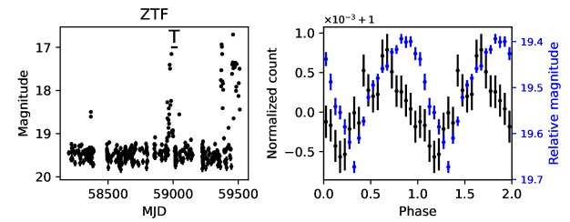
Figure 15: Left: The light curve of G454 measured by ZTF (ZTF18abttrrr). The outburst occurred at 2021, September as reported as a GAIA transient source, AT 2021aath (GAIA21eni). Right : ZTF (blue) and TESS (black) light curves folded with a frequency of $f_{ZTF}=8.6499~{}{\rm day^{-1}}$ ($\sim 0.12$ day), and the phase zero refers MJD 59398.713391. The TESS observation was carried out around MJD 58980-5904 during the outburst.

GAIA DR2 4321588332240659584 (hereafter G432) is selected as a candidate for a counterpart of the Swift point source, 2SXPS J192530.4+155424, and the X-ray luminosity is measured as $L_{X}\sim 1.4^{+2.4}_{-0.8}\times 10^{32}(d/582~{}{\rm pc})^{2}{\rm erg~{}cm^{-2}s^{-1}}$ in the 0.3-10 keV band (Table 3). As compared with the ZTF light curves of other candidates in this study, the optical emission from this source (ZTF18aazmehw) is more steady with an amplitude of variation of less than $\sim$1 mag (right panel of Figure 13). In the LS-periodogram of the ZTF light curve, we confirm a periodic signal at a frequency of $f_{ZTF}=18.5521(9)~{}{\rm day^{-1}}$ ($\sim 0.054$ day).

TESS observed the region around G432 in 2019, July (sector 14) and 2021, June (sector 40), for which data were taken approximately every $30$ minutes and $\sim 10$ minutes, respectively. Figure 14 shows LS-periodogram for the data of sectors 14 and 40. The LS-periodogram (left panel) clearly indicates a periodic signal at $F_{0}=18.553(1)~{}{\rm day^{-1}}$, which is consistent with the finding from ZTF. The folded light curve with $f_{ZTF}$ (right panel of Figure 14) may be described by the main peak plus a small secondary, rather than a pure sinusoidal curve, although the significance of the secondary peak is small. In the LS-periodogram, we can see the signals at the second harmonics ($F_{1}=2F_{0}$) and the effect of aliasing with the data sampling frequency of $F_{s}\sim 145~{}{\rm day^{-1}}$, namely $F_{b}=F_{s}-F_{0}\sim 126~{}{\rm day^{-1}}$ and $F_{b1}=F_{s}-F_{1}\sim 108~{}{\rm day^{-1}}$

In addition to the periodic signals related to $F_{0}$ and $2F_{0}$, the periodogram shows other signals at $F_{u}=32.17(4)~{}{\rm day^{-1}}$ ($\sim 0.031$ day) and its harmonics $F_{u}/2$. This signal clearly appears in the TESS data of the sector 40. To check which pixel of the TESS-FFIs causes the signal, we extract the light curve of each pixel around the sources for the observation of sector 40. We find that a significant signal with $F_{u}$ can be detected at one pixel where the power of the signal with $F_{0}$ becomes the maximum. The periodic signal with $F_{0}$ can be seen in other pixels but the power of the signal is lower than that at the pixel where the $F_{u}$ signal is found. Hence, the signal, $F_{u}$, may be related to our target, although other optical sources located in the same pixel (right panel of Figure 13) cannot be ruled out as the origin of the signal. We note that LS periodogram of TESS data is insensitive to the time-correlated noise model discussed in Appendix A.

If the signal $F_{u}$ is related to G432, then the origin may be related to the harmonics of $F_{0}$. Although the frequency $F_{u}=32.17(4)~{}{\rm day^{-1}}$ cannot be described by a simple relation with $F_{0}$, the frequency $F_{s}-F_{u}\sim 6F_{0}$, where $F_{s}\sim 145~{}{\rm day^{-1}}$ is the data readout frequency, indicates that the signal $F_{u}$ is related to the 6th harmonic of the fundamental frequency. It is not trivial, however, why the modulation of the 6th harmonic is more evident than those of the 2nd-5th harmonics. If the frequency $F_{u}$ is independent of $F_{0}$, the signal would be related to the spin of the WD. We cannot find a significant periodic signal at the frequency $F_{u}$ in the data of sector 14. This may be due to a large uncertainty of each data point of the observation or the true signal is $F_{s}-F_{u}\sim 111~{}{\rm day^{-1}}$ ($\sim 13$ minutes) for which the data of sector 14 cannot identify. If $F_{u}$ and $F_{0}$ are related to the WD spin and orbital period, respectively, G432 could be a candidate for IP due to the fact that the X-ray emission dominates the UV emission, which is a typical property of the emission of IPs (section 4.1). A data set taken with a higher cadence is required to identify the origin of $F_{u}$.

3.5 GAIA DR2 4542123181914763648

We select GAIA DR2 4542123181914763648 (hereafter G452) as a candidate of the optical counterpart of 1RXS J172728.8+132601, for which a 2.5 ks Swift observation measures the X-ray luminosity of $L_{X}=5.5^{+14}_{-3.2}\times 10^{31}(d/502{\rm pc})^{2}~{}{\rm erg~{}s^{-1}}$ with $N_{H}=7.5\times 10^{21}~{}{\rm cm^{2}}$ (Table 3). As the ZTF light curve (ZTF18abttrrr) shows (left panel of Figure 15), the source repeats outbursts on a time scale of years; the outburst happened in 2021 was alerted as a GAIA transient source, AT 2021aath (GAIA21eni, Hodgkin et al., 2021), which was identified as a polar type CV. Nevertheless, since there is no detailed binary information for the target in the literature, we search for a possible periodic signal in the ZTF light curve. After removing the data of the outburst from the light curve, the LS-periodogram shows a significant periodic signal at $f_{ZTF}=8.6499(8)~{}{\rm day^{-1}}$ ($\sim 0.115$ day).

TESS observation for the region around G452 was carried out in 2020, May and June (sectors 25 and 26) during the outburst around MJD 59000 (Figure 15). We extracted the TESS-FFI light curve and removed a long-term trend caused by the outburst from the light curve. We found a periodic signal with $F_{0}=8.65(2)~{}{\rm day^{-1}}$, which is consistent with the result of the ZTF observation. The right panel of Figure 15 shows the folded light curves of the ZTF and TESS data, which can be described by a sinusoidal modulation. As Figure 15 shows, we also observe a shift in the TESS light curve from the ZTF light curve, which may be due to the effect of an outburst during the TESS observation. We do not find another significant periodic signal in the TESS data, which may be consistent with a spin-orbit phase synchronization of the polar.

3.6 Other candidates

We searched for a possible periodic signal of 29 GAIA DR2 sources, which are potential counterparts of an unidentified X-ray source. Table 4 presents four sources, for which TESS-FFI data provides a periodic signal, but no enough data points or no data are available for ZTF observations. As we have mentioned, there are two observational modes for TESS-FFIs, in which the data readout time intervals are $\sim 48~{}{\rm day^{-1}}$ and $\sim 144~{}{\rm day^{-1}}$, respectively. As shown in Table 4, GAIA DR2 5360633963010856448 and 5964753754945126528 were observed by two observational modes, and the periodic signal $F_{0}$ reported in Table 4 is identified in both data sets. For GAIA DR2 2031371479242995584 and  1981213682883140864, on the other hand, data from only one observational mode is available, and we cannot discriminate between the true frequency and the aliasing. We note that due to one pixel of the TESS observations containing several GAIA sources, we cannot rule out that the periodic signal is related to another source.

Among the four sources in Table 4, GAIA DR2 5964753754945126528 (hereafter G596), which shows a periodic signal $F_{0}\sim 8.34~{}{\rm day^{-1}}$ $(\sim 0.120$ day) in the TESS data, is a promising candidate for a CV, and its location is consistent with the X-ray source, AX J1654.3-4337, which was discovered by the ASCA Galactic plane survey (Sugizaki et al., 2001). Swift and NuSTAR observations for this source were carried out in 2020 July-August with a total exposure of 6.7 ks and 26 ks, respectively. We extract the events and spectra of the source region with the command nupipeline under HEASoft ver.6-29 for the NuSTAR data and the package Xselect for the Swift data.

We group the spectral bins to contain a minimum of 20 counts in each bin, and fit the spectrum using Xspec ver.12.12 (Figure 16). We find that the spectrum in the 0.2-70 keV band is well fitted by the optically thin thermal plasma emission (tbabs*mekal model in Xspec) with a temperature of $k_{B}T=8.9^{+2.0}_{-1.5}$ keV and absorption column density of $N_{H}=2.2^{+0.08}_{-0.07}\times 10^{21}~{}{\rm cm^{-2}}$ ($\chi^{2}=164$ for 188 D.O.F.). The luminosity in the 0.2-70 keV band is estimated to be $L_{X}=6.0^{+0.6}_{-0.5}\times 10^{31}(d/462~{}{\rm pc})^{2}~{}{\rm erg~{}s^{-1}}$. The X-ray emission with a plasma temperature of $\sim 10$ keV suggests the emission from an accretion column on the WD surface, indicating a magnetic CV system. Moreover, the observed X-ray luminosity of $<10^{32}~{}{\rm erg~{}s^{-1}}$ indicates that the source is not a typical IP, for which the X-ray luminosity is typically $>10^{32}~{}{\rm erg~{}s^{-1}}$.

Figure 17 presents the folded light curve of $F_{0}=8.34~{}{\rm day^{-1}}$ extracted from the TESS-FFI data. We can see that the shape of light curve shows a double-peak structure. Combined with the X-ray spectral properties, this optical emission likely originated from two magnetic poles heated by the accretion column, and the modulation is likely due to the WD spin. Since the TESS data did not indicate other periodic signals longer than this WD’s spin signal within 10 day, G596/AX J1654.3-4337 may be a polar, although we cannot rule out the possibility of an IP. We do not find any periodic signal in the NuSTAR data, in which a window effect of the observation dominates the LS-periodogram.

Table 4: Other CV candidates

GAIA	X-ray source	Distance	TESS	$F_{0}$	Proposed type
DR2		(pc)	Sector	(${\rm day^{-1}}$)
5360633963010856448	1RXS J104612.9-511819	496	10, 36, 37	15.46(2)
5964753754945126528	2SXPS J165423.6-433745	462	12, 39	8.34(4)	Polar
	AX J1654.3-4337 (AX1654)
2031371479242995584	1RXS J194401.5+284456	416	40, 41	4.20/139.8
1981213682883140864	2SXPS J220344.5+525450	754	16, 17	1.15/46.85

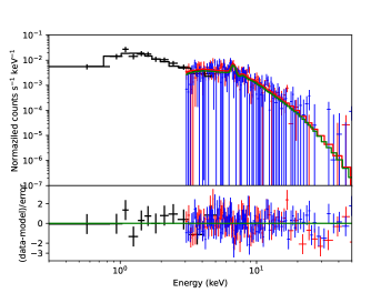
Figure 16: Swift (black) and NuSTAR (red and blue) spectra of AX J1654.3-4337, which will be the X-ray counterpart of GAIA DR2 5964753754945126528. The spectrum is described by an optically thin thermal plasma emission with a temperature of $k_{B}T\sim 8.9$ keV.

Figure 17: TESS light curve of G596/AX J1654.3-4337 folded with $F_{0}=8.34~{}{\rm day^{-1}}$ $(\sim 0.12~{}{\rm day})$. The phase zero refers MJD 59398.713391.

4 Discussion and summary

4.1 Comparison with known CVs

Figure 18: Distributions of GAIA G-band magnitudes (top) or X-ray luminosity in the 0.3-10 keV band with the orbital period: For G453, G205 and G432, the orbital period is assumed to be $F_{0}$ measured by TESS, although true period of $F_{0}/2$ cannot be ruled out. The back, blue and red filled circles correspond to nonmagnetic CV, polar and IP, respectively, as listed in Ritter Cataclysmic Binaries Catalog (Ritter & Kolb, 2003). The diamond and green box symbols represent CV candidates and AR Scorpii, respectively. The X-ray luminosity is calculated from the flux and parallax measured by Swift (Evans et al., 2020) and GAIA, respectively.

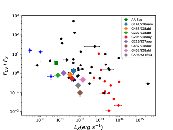
Figure 19: Distribution of UV/X-ray flux ratio with the X-ray luminosity measured by the Swift observation. The back-, blue-, and red-filled circles correspond to no-magnetic CV, polar, and IP, respectively.

Figures 18 and 19 compare the properties of our CV candidates with those of known CVs. Figure 18 shows the distributions of the orbital periods and GAIA G-bands magnitudes (upper panel) or the X-ray luminosity in the 0.3-10 keV band (lower panel) of our candidates. In the figure, we can see so-called period gap at $P_{orb}\sim 2-3$ hr, in which less CVs have been detected (Spruit & Ritter, 1983; Ritter, 2010; Katysheva & Pavlenko, 2003; Garraffo et al., 2018). The figure shows that the nonmagnetic systems (black-filled circle) have been detected with a period in the range of 0.01-1 day. Known IPs (red-filled circle) and polars (blue filled circle), on the other hand, concentrate on the orbital periods longer and shorter than the period gap, respectively. We find in the figure that the six CV candidates discussed in the current study are located below the period of the gap. This will be a selection effect because (i) there is a correlation between the orbital period and GAIA G-band magnitudes, as seen in top panel of Figure 18, and (ii) we have selected the candidates with the condition $9<M_{G}<12$ of the G-bands magnitude (Figure 1). AX J1654.3-4337 (pink diamond), which is a polar candidate as discussed in section 3.6, locates in or close to the period gap. As the bottom panel of Figure 18 shows, the X-ray luminosity of our candidate, $L_{X}\sim 10^{31-32}~{}{\rm erg~{}s^{-1}}$ is relatively larger among the CVs located below the period gap. This is because we searched candidates in the X-ray source catalogs of previous surveys, which may have miss many faint X-ray sources.

We can see in the figure that four candidates (G453, G205, G216, and G432) have an orbital period close to or shorter than $\sim 0.05$ day, which is known as the minimum orbital period in the standard binary evolution of CVs (Ritter, 2010). We note however that the orbital periods of G453, G205 and G432 may be double the values in the figure (sections 3.3 and 3.4), and hence they may have an orbital period longer than the minimum period.

Figure 19 shows the distribution of the flux ratio of the UV band and X-ray band measured by Swift. As can be seen in the figure, the ratio is greater than unity for most of the nonmagnetic system, which is understood by the emission from the boundary layer of the accretion disk. For magnetic CVs, on the other hand, the X-ray dominates the UV emission, which is a characteristic of emission from the accretion column (Mukai, 2017). Several sources, on the other hand, have a ratio greater than 10, and the emission is probably dominated by blackbody emission from the pole with a temperature of $<50$ eV.

We find that our candidates have relatively hard spectrum ($F_{UV}/F_{X}\leq 1$) and the two hardest sources (G432 and G596) are classified as candidates for magnetic CVs. For G432, we identify two possible periodic signals ($F_{0}=18.5~{}{\rm day^{-1}}$ and $F_{u}=32.2$ or $111~{}{\rm day^{-1}}$) in the TESS data. With the UV/X flux ratio much smaller than unity, G432 may be a candidate of X-ray faint IP. For G596, the properties of the optical light curve and the X-ray spectrum are consistent with a polar, as described in section 3.6.

In the unidentified X-ray source, we searched for new binary candidates that show emission properties similar to those of AR Scorpii, for which (i) no mass is probably transferred from the companion star to the WD, (ii) UV emission dominates the X-ray emission, and (iii) a magnetic WD heats up the companion star. With current photometric studies, however, we can conclude that these candidates do not belong to the AR Scorpii-type binary system. For example, three candidates (G141, G453 and G454) clearly show dwarf-nova-type outbursts, suggesting the existence of a mass transfer from the companion to the WD, and thus an accreting system. With a large optical variation ($\delta m\sim 1.5$), AR Scorpii contains a WD heating up the companion star. The optical curves of our candidates show a smaller magnitude variation ($\delta m<1$, e.g. Figure 12 for G216 and Figure 13 for G432), and do not show any clear evidence of heating. G596/AX J1654.3-4337 is a promising candidate for the magnetic system, but it is a polar, while AR Scorpii is an IP in the sense that the spinning period is different from the orbital period.

Finally, we note that out of our eight candidates, six systems have not experienced a large outburst in the last 4 years, and have been missed in the previous surveys. Our study, therefore, will suggest that a large population of WD binary systems with an inactive mass transfer could be discovered in future surveys.

In summary, we searched for new CV systems associated with the unidentified X-ray sources listed in ROSAT, Swift and XMM-Newton source catalogs. We selected the GAIA sources with a g-band magnitude of $9<M_{G}<12$ and a color $0.5<G_{BP}-G_{RP}<1.5$, and identified 29 sources that are potential counterparts of the unidentified X-ray sources. We carried out a photometric study with ZTF, TESS and LOT observations, and we constrained the orbital periods for the seven sources (sections 3.1-3.5). Among the seven candidates, G141 and G207 are eclipsing binary systems, and G141 shows a secondary eclipse with a shallower depth. We identified three candidates (G141, G453 and G454), in which a mass transfer from the companion to WD is active, and they exhibit repeated outbursts (Figures 2, 6 and 15). For the other three candidates (G207, G205, and G216), on the other hand, it is observed that the source brightness suddenly drops and stays at a low luminous state (Figure 10), suggesting the mass transfer may be inactive. Based on the detection of two periodic signals in the light curve and UV/X-ray emission properties, we can classify G141 and G432 as IP candidates, although a spectroscopic study is required for confirmation. In addition to seven candidates, we confirmed that the unidentified ASKA source, AX J1654.3-4337 (G569), is a candidate for being a polar. With the current photometric studies, we could not find any candidate for the AR Scorpii-type WD binary, although we selected the GAIA sources that had a similar magnitude to AR Scorpii. AR Scorpii still remains a n unique WD binary system, and a more sophisticated search (e.g. an optical survey for unidentified X-ray source with high cadence) will be required to find a new AR Scorpii-type binary system.

We thank to referee for his/her useful comments and suggestions. We are grateful to Dr. Kato for providing the source list in VSX catalog and sending some references. We also thank the Swift-TOO team for arranging the observations for our sources. J.T. and X.F.W are supported by the National Key Research and Development Program of China (grant No. 2020YFC2201400) and the National Natural Science Foundation of China (grant No. 12173014). A.K.H.K. is supported by the Ministry of Science and Technology (MOST) of Taiwan through grant Nos. 108-2628-M-007- 005-RSP and 109-2628-M-007-005-RSP. J.M. is supported by the National Natural Science Foundation of China (grant No. 11673062). C.-P.H. acknowledges support from the MOST of Taiwan through grant MOST 109-2112-M-018-009-MY3. L.C.-C.L. is supported by MOST through grant MOST 110-2811-M-006-515 and MOST 110-2112-M-006-006-MY3. K.-L. L. is supported by the MOST of Taiwan through grant 110-2636-M-006-013, and he is a Yushan (Young) Scholar of the Ministry of Education of Taiwan. C. Y. H. is supported by the National Research Foundation of Korea through grant 2016R1A5A1013277 and 2019R1F1A1062071.

Note added in proof: While this article in press, we were noticed that potential orbital periods of 4 sources have been already reported in the AAVSO catalog (for 2SXPS J202600.8+333940 and 2SXPS J192530.4+155424) or in vsnet-chat (for 4XMM J172959.0+522948 and 2SXPS J195230.9+372016). We list references of the AAVSO catalogs and archives of vsnet-chat for the 7 sources listed in Table 1. In Appendix C (for manuscript in archive), we briefly mention the information in the catalog and compare with our results.

ZTF18aampffv=4XMM J172959.0+52294=MGAB-V705 https://www.aavso.org/vsx/index.php?view
=detail.top&oid=1499054
http://ooruri.kusastro.kyoto-u.ac.jp/mailarchive/
vsnet-chat/8923

ZTF18abikbmj=1RXS J185013.9+242222=DDE163 https://www.aavso.org/vsx/index.php?view=detail.top&oid=686692

ZTF18abrxtii=2SXPS J195230.9+372016
https://www.aavso.org/vsx/index.php?view=detail.top&oid=2224634
http://ooruri.kusastro.kyoto-u.ac.jp/mailarchive/vsnet-chat/8866

ZTF18aayefwp=2SXPS J202600.8+333940=BMAM-V634 https://www.aavso.org/vsx/index.php?view=detail.top&oid=1543125
http://ooruri.kusastro.kyoto-u.ac.jp/mailarchive/vsnet-chat/8920

ZTF17aaapwae=2SXPS J211129.4+445923
https://www.aavso.org/vsx/index.php?view=detail.top&oid=2223038

ZTF18aazmehw=2SXPS J192530.4+155424=DDE182 https://www.aavso.org/vsx/index.php?view=detail.top&oid=1543028

ZTF18abttrrr=1RXS J172728.8+132601=GAIA21eni
https://www.aavso.org/vsx/index.php?view=detail.top&oid=2224470

Swift(XRT), XMM-Newton(EPIC), NuSTAR(FPM), ZTF, TESS and LOT.

Appendix A LS periodogram with time-correlated noise model

We apply the time-correlated noise model based on Equation (13) of Delisle et al. (2020), and assume the covariance matrix to follow

$$C_{i,j}=\delta_{i,j}\sigma_{i}^{2}+\sigma^{2}_{\rm exp}e^{|t_{i}-t_{j}|/\tau_{\rm exp}},$$ (A1)

where $\sigma_{i}$ is the diagonal matrix with the observational error bars that are usually provided in the processed data, and $\sigma_{\rm exp}$ corresponds to the correlated noise with a time scale of $\tau_{exp}$. We choose the amplitude of the fluctuation in the light curve to be $\sigma_{\rm exp}$, and create the periodogram for the different values of $\tau_{\rm exp}$. For each frequency, the normalized power of the LS periodogram is calculated from (VanderPlas, 2018)

$$z_{1}(f)=1-\frac{\hat{\chi}^{2}(f)}{\hat{\chi}^{2}_{0}},$$ (A2)

where $\hat{\chi}^{2}$ is the minimum value of $\chi^{2}(f)=(\mathbf{y}-\mathbf{y}_{\rm model})^{T}\mathbf{C}^{-1}(\mathbf{y}-\mathbf{y}_{\rm model})$, and $\mathbf{y}$ and $\mathbf{y}_{\rm model}$ are the time series of the observation and model, respectively. In addition, $\hat{\chi}^{2}_{0}$ is a non-varying reference value. For each periodogram, we scan the frequency between $1~{}{\rm day^{-1}}<f<100~{}{\rm day^{-1}}$ and estimate FAP using the method of Delisle et al. (2020). We can see that the LS periodogram of TESS data is insensitive to the time-correlated noise model within the current framework.

Figure 20 shows the LS periodogram of the ZTF data with the time-correlated noise model for G141 (left panel) and G205 (right panel). As we demonstrated in section 3.1, the possible periodic signal, $f_{ZFT}\sim 47~{}{\rm day^{-1}}$, of G141 cannot be confirmed in the TESS/LOT data. From the left panel of Figure 20, we find that the signal at $f_{ZFT}\sim 47~{}{\rm day^{-1}}$ disappears from LS periodogram for $\tau_{exp}>0.1$ day. For G205 (right panel), on the other hand, the periodic signal $f_{ZTF}\sim 24.6~{}{\rm day^{-1}}$ is confirmed in the TESS data, and the existence of the signal in the periodogram is insensitive to the noise model. Although the noise model affects the shape of the LS periodogram of the ZTF data, it is less effective in determining the existence of the periodic signal reported in Table 1. These results suggest that the periodic signal $f_{ZFT}\sim 47~{}{\rm day^{-1}}$ of G141 is likely related to the time-correlated noise.

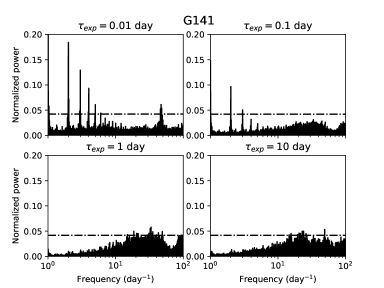
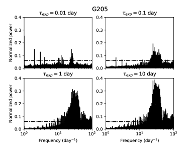
Figure 20: LS periodograms with correlated noise models (A1) for G141 (left) and G205 (right). The results are for $\sigma_{exp}=1$ magnitude. The dashed-dotted lines represent FAT=0.01 estimated from the method of Delisle et al. (2020).

Appendix B LS-periodograms and folded light curves of ZTF and TESS data

Figures 22 and 23 show LS-periodograms of the TESS data and folded light curves of ZTF/ TESS data for seven candidates listed in Table 1. Figure 24 presents the LS-periodograms and folded light curves of TESS data for the four candidates listed in Table 4.

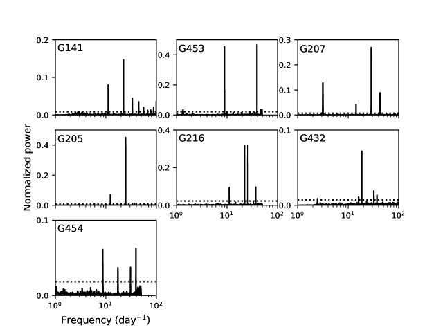
Figure 22: The LS-periodograms of the TESS data for the seven candidates listed in Table 1 with Gaussian and time uncorrelated noise model [the first term in equation of (20)]. The dotted horizontal lines represent FAP=0.01 estimated from the bootstrap method.

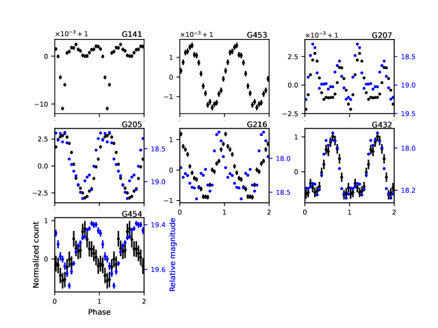
Figure 23: ZTF (blue color) and TESS (black color) light curves for seven candidates in Table 1. The data is folded with $f_{ZTF}$ (or $F_{0}$), except for $F_{0}/2$ of G207. For G141 and G453, the ZTF data do not show a periodic signal of $F_{0}$. Phase zero corresponds to MJD 59398.713391, and two cycles are plotted for clarity.

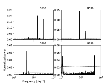
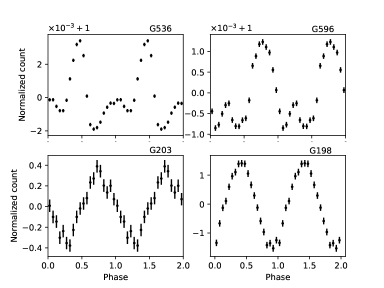
Figure 24: The LS-periodograms (left) and folded light curves (right) of the TESS data for the four candidates listed in Table 4. The dotted lines in the left panel show FAP=0.01 estimated with the bootstrap method. In the right panel, phase zero corresponds to MJD 59398.713391, and two cycles are plotted for clarity.

Appendix C Information from the International Variable Star Index and vsnet-chat

While the article in press, we were noted that the candidates of the orbital periods for 4 sources in 7 candidates listed in in Table 1 have been reported in the international Variable Star Index (VSX, for G205 and G432) and in vsnet-chat (for G141 and G207). We summarize the information in VSX and vsnet-chat for 7 sources.

G141,4XMM J172959.0+522948

This source is named as MGAB-V705 in VSX and the candidate of orbital period $\sim 0.0897008(1)$ day is reported in vsnet-chat 8923. This value is consistent with the value reported in Table 1.

G453, 1RXS J185013.9+242222

As noted in main text, this source has been known as a dwarf nova by previous observation of the outburst. This source is named as DDE 163 in VSX

G207, 2SXPS J195230.9+372016

This source is counterpart of ZTF 18abrxtii, which is listed in VSX. The orbital period $\sim 0.0699896(1)$ day, which is consistent with the value reported in Table 1, is mentioned in vsnet-chat 8866.

G205, 2SXPS J202600.8+333940

This source is named as BMAM-V634 in VSX, and the candidate of orbital period $\sim$0.0813141 day obtained from ZTF data (Chen et al., 2020) is consistent with our result.

G216, 2SXPS J211129.4+445923

This source is counter part of ZTF 17aaapwae, which is listed in VSX as a variable star.

G432, 2SXPS J192530.4+155424

This source is named as DDE 182 in VSX. The candidate of the orbital period $\sim 0.053903$ day in the catalog is consistent with our result.

G454, 1RXS J172728.8+132601

As noted in the main text, the outburst happened in 2021 was alerted as a GAIA transient source, AT 2021. ZTF 18abttrrr is listed in VSX as a variable star.

References

- Aleksić et al. (2014) Aleksić, J., Ansoldi, S., Antonelli, L. A., et al. 2014, A&A, 568, A109
- Arnaud (1996) Arnaud, K. A. 1996, in Astronomical Society of the Pacific Conference Series, Vol. 101, Astronomical Data Analysis Software and Systems V, ed. G. H. Jacoby & J. Barnes, 17
- Ashley et al. (2020) Ashley, R. P., Marsh, T. R., Breedt, E., et al. 2020, MNRAS, 499, 149
- Astropy Collaboration et al. (2013) Astropy Collaboration, Robitaille, T. P., Tollerud, E. J., et al. 2013, A&A, 558, A33
- Baluev (2008) Baluev, R. V. 2008, MNRAS, 385, 1279
- Brasseur et al. (2019) Brasseur, C. E., Phillip, C., Fleming, S. W., Mullally, S. E., & White, R. L. 2019, Astrocut: Tools for creating cutouts of TESS images, ascl:1905.007
- Buckley et al. (2017) Buckley, D. A. H., Meintjes, P. J., Potter, S. B., Marsh, T. R., & Gänsicke, B. T. 2017, Nature Astronomy, 1, 0029
- Chen et al. (2020) Chen, X., Wang, S., Deng, L., et al. 2020, ApJS, 249, 18
- Coppejans et al. (2016) Coppejans, D. L., Körding, E. G., Knigge, C., et al. 2016, MNRAS, 456, 4441
- Delisle et al. (2020) Delisle, J. B., Hara, N., & Ségransan, D. 2020, A&A, 635, A83
- Evans et al. (2020) Evans, P. A., Page, K. L., Osborne, J. P., et al. 2020, ApJS, 247, 54
- Feinstein et al. (2019) Feinstein, A. D., Montet, B. T., Foreman-Mackey, D., et al. 2019, PASP, 131, 094502
- Gabriel et al. (2004) Gabriel, C., Denby, M., Fyfe, D. J., et al. 2004, in Astronomical Society of the Pacific Conference Series, Vol. 314, Astronomical Data Analysis Software and Systems (ADASS) XIII, ed. F. Ochsenbein, M. G. Allen, & D. Egret, 759
- Gaia Collaboration et al. (2018) Gaia Collaboration, Babusiaux, C., van Leeuwen, F., et al. 2018, A&A, 616, A10
- Garnavich et al. (2021a) Garnavich, P., Littlefield, C., Lyutikov, M., & Barkov, M. 2021a, ApJ, 908, 195
- Garnavich et al. (2021b) Garnavich, P., Littlefield, C., Wagner, R. M., et al. 2021b, ApJ, 917, 22
- Garraffo et al. (2018) Garraffo, C., Drake, J. J., Alvarado-Gomez, J. D., Moschou, S. P., & Cohen, O. 2018, ApJ, 868, 60
- Ginsburg et al. (2019) Ginsburg, A., Sipőcz, B. M., Brasseur, C. E., et al. 2019, AJ, 157, 98
- Hameury (2020) Hameury, J. M. 2020, Advances in Space Research, 66, 1004
- Hodgkin et al. (2021) Hodgkin, S. T., Breedt, E., Delgado, A., et al. 2021, Transient Name Server Discovery Report, 2021-3431, 1
- Imada et al. (2012) Imada, A., Izumiura, H., Kuroda, D., et al. 2012, PASJ, 64, L5
- Jackim et al. (2020) Jackim, R., Szkody, P., Hazelton, B., & Benson, N. C. 2020, Research Notes of the American Astronomical Society, 4, 219
- Kato et al. (2010) Kato, T., Maehara, H., Uemura, M., et al. 2010, PASJ, 62, 1525
- Kato et al. (2014) Kato, T., Dubovsky, P. A., Kudzej, I., et al. 2014, PASJ, 66, 90
- Katysheva & Pavlenko (2003) Katysheva, N. A., & Pavlenko, E. P. 2003, Astrophysics, 46, 114
- Katz (2017) Katz, J. I. 2017, ApJ, 835, 150
- Kitaguchi et al. (2014) Kitaguchi, T., An, H., Beloborodov, A. M., et al. 2014, ApJ, 782, 3
- Li et al. (2016) Li, J., Torres, D. F., Rea, N., et al. 2016, ApJ, 832, 35
- Lightkurve Collaboration et al. (2018) Lightkurve Collaboration, Cardoso, J. V. d. M., Hedges, C., et al. 2018, Lightkurve: Kepler and TESS time series analysis in Python, Astrophysics Source Code Library, ascl:1812.013
- Lindegren et al. (2018) Lindegren, L., Hernández, J., Bombrun, A., et al. 2018, A&A, 616, A2
- Lomb (1976) Lomb, N. R. 1976, Ap&SS, 39, 447
- Lopes de Oliveira et al. (2020) Lopes de Oliveira, R., Bruch, A., Rodrigues, C. V., Oliveira, A. S., & Mukai, K. 2020, ApJ, 898, L40
- Lyutikov et al. (2020) Lyutikov, M., Barkov, M., Route, M., et al. 2020, arXiv e-prints, arXiv:2004.11474
- Marsh et al. (2016) Marsh, T. R., Gänsicke, B. T., Hümmerich, S., et al. 2016, Nature, 537, 374
- Masci et al. (2019) Masci, F. J., Laher, R. R., Rusholme, B., et al. 2019, PASP, 131, 018003
- Meintjes et al. (1994) Meintjes, P. J., de Jager, O. C., Raubenheimer, B. C., et al. 1994, ApJ, 434, 292
- Mukai (2017) Mukai, K. 2017, PASP, 129, 062001
- Nasa High Energy Astrophysics Science Archive Research Center (2014) (Heasarc) Nasa High Energy Astrophysics Science Archive Research Center (Heasarc). 2014, HEAsoft: Unified Release of FTOOLS and XANADU, ascl:1408.004
- Osaki (2005) Osaki, Y. 2005, Proceedings of the Japan Academy, Series B, 81, 291
- Patterson (1979) Patterson, J. 1979, ApJ, 234, 978
- Patterson et al. (2000) Patterson, J., Kemp, J., Jensen, L., et al. 2000, PASP, 112, 1567
- Pelisoli et al. (2022) Pelisoli, I., Marsh, T. R., Dhillon, V. S., et al. 2022, MNRAS, 509, L31
- Pretorius et al. (2021) Pretorius, M. L., Hewitt, D. M., Woudt, P. A., et al. 2021, MNRAS, 503, 3692
- Ricker et al. (2014) Ricker, G. R., Winn, J. N., Vanderspek, R., et al. 2014, in Society of Photo-Optical Instrumentation Engineers (SPIE) Conference Series, Vol. 9143, Space Telescopes and Instrumentation 2014: Optical, Infrared, and Millimeter Wave, ed. J. Oschmann, Jacobus M., M. Clampin, G. G. Fazio, & H. A. MacEwen, 914320
- Ritter (2010) Ritter, H. 2010, Mem. Soc. Astron. Italiana, 81, 849
- Ritter & Kolb (1998) Ritter, H., & Kolb, U. 1998, A&AS, 129, 83
- Ritter & Kolb (2003) —. 2003, A&A, 404, 301
- Schreiber et al. (2021) Schreiber, M. R., Belloni, D., Gänsicke, B. T., Parsons, S. G., & Zorotovic, M. 2021, Nature Astronomy, 5, 648
- Spruit & Ritter (1983) Spruit, H. C., & Ritter, H. 1983, A&A, 124, 267
- Stanway et al. (2018) Stanway, E. R., Marsh, T. R., Chote, P., et al. 2018, A&A, 611, A66
- Sugizaki et al. (2001) Sugizaki, M., Mitsuda, K., Kaneda, H., et al. 2001, ApJS, 134, 77
- Sun et al. (2021) Sun, Y., Cheng, Z., Ye, S., et al. 2021, arXiv e-prints, arXiv:2111.13049
- Szkody et al. (2021) Szkody, P., Olde Loohuis, C., Koplitz, B., et al. 2021, AJ, 162, 94
- Takata et al. (2018) Takata, J., Hu, C. P., Lin, L. C. C., et al. 2018, ApJ, 853, 106
- Takata et al. (2017) Takata, J., Yang, H., & Cheng, K. S. 2017, ApJ, 851, 143
- Terada et al. (2008) Terada, Y., Hayashi, T., Ishida, M., et al. 2008, PASJ, 60, 387
- Tody (1993) Tody, D. 1993, in Astronomical Society of the Pacific Conference Series, Vol. 52, Astronomical Data Analysis Software and Systems II, ed. R. J. Hanisch, R. J. V. Brissenden, & J. Barnes, 173
- VanderPlas (2018) VanderPlas, J. T. 2018, ApJS, 236, 16
- Voges et al. (1999) Voges, W., Aschenbach, B., Boller, T., et al. 1999, A&A, 349, 389
- Warner (1995) Warner, B. 1995, Cataclysmic variable stars, Vol. 28
- Webb et al. (2020) Webb, N. A., Coriat, M., Traulsen, I., et al. 2020, A&A, 641, A136
- Wilson et al. (2021) Wilson, D. J., Toloza, O., Landstreet, J. D., et al. 2021, MNRAS, 508, 561
- Wynn et al. (1997) Wynn, G. A., King, A. R., & Horne, K. 1997, MNRAS, 286, 436
- Zhao et al. (2006) Zhao, Y., Li, Z., Wu, X., et al. 2006, PASJ, 58, 367