Fast Hierarchical Deep Unfolding Network for
Image Compressed Sensing

Abstract.

By integrating certain optimization solvers with deep neural network, deep unfolding network (DUN) has attracted much attention in recent years for image compressed sensing (CS). However, there still exist several issues in existing DUNs: 1) For each iteration, a simple stacked convolutional network is usually adopted, which apparently limits the expressiveness of these models. 2) Once the training is completed, most hyperparameters of existing DUNs are fixed for any input content, which significantly weakens their adaptability. In this paper, by unfolding the Fast Iterative Shrinkage-Thresholding Algorithm (FISTA), a novel fast hierarchical DUN, dubbed FHDUN, is proposed for image compressed sensing, in which a well-designed hierarchical unfolding architecture is developed to cooperatively explore richer contextual prior information in multi-scale spaces. To further enhance the adaptability, series of hyperparametric generation networks are developed in our framework to dynamically produce the corresponding optimal hyperparameters according to the input content. Furthermore, due to the accelerated policy in FISTA, the newly embedded acceleration module makes the proposed FHDUN save more than 50% of the iterative loops against recent DUNs. Extensive CS experiments manifest that the proposed FHDUN outperforms existing state-of-the-art CS methods, while maintaining fewer iterations.

1. Introduction

Compressed sensing (CS)(Donoho, 2006; Candès and Wakin, 2008) theory demonstrates that if a signal is sparse in a certain domain, it can be recovered with a high probability from a much fewer acquired measurement than prescribed by the Nyquist sampling theorem. Recently, the benefits of its reduced sampling rate have attracted many practical applications, including but not limited to single-pixel imaging(Duarte et al., 2008; Rousset et al., 2017), magnetic resonance imaging (MRI)(Lustig et al., 2008; Mardani et al., 2019) and snapshot compressive imaging(Liu et al., 2019; Miao et al., 2019).

Mathematically, given the input signal $x\in\mathbb{R}^{N}$, the sampled linear measurements $y\in\mathbb{R}^{M}$ can be obtained by $y=\Phi x$, where $\Phi\in\mathbb{R}^{M\times N}$ is the sampling matrix with $M\ll N$ and $\frac{M}{N}$ is the CS sampling ratio. Obviously, the signal recovery from the compressed measurements is to solve an under-determined linear inverse problem(Shi et al., 2020), and the corresponding optimization model can be formulated as follows:

(1) $$\tilde{x}=\mathop{\arg}\mathop{\min}_{x}\frac{1}{2}\|\Phi x-y\|_{2}^{2}+\lambda\psi(x)\vspace{-0.04in}$$

where $\psi(x)$ is the prior term with the regularization parameter $\lambda$. In the traditional CS methods(Gao et al., 2015; Kim et al., 2010; Metzler et al., 2016; Chen et al., 2011), the prior term can be the sparsifying operator in certain pre-defined transform domains (such as DCT(Zhao et al., 2014) and wavelet(Anselmi et al., 2015)). To further enhance the reconstructed quality, more sophisticated structures are established, including minimal total variation(Candes et al., 2006; Li et al., 2013), low rank(Dong et al., 2014; Golbabaee and Vandergheynst, 2012) and non-local self-similarity image prior(Zha et al., 2020; Zhang et al., 2014). Many of these approaches have led to significant improvements. However, these optimization-based CS reconstruction algorithms usually suffer from high computational complexity because of their hundreds of iterations, thus limiting the practical applications of CS greatly.

Recently, fueled by the powerful learning ability of deep neural networks, many deep network-based image CS methods have been proposed. According to the intensity of interpretability, the existing CS networks can be roughly grouped into the following two categories: Uninterpretable deep black box CS network (DBN) and interpretable deep unfolding CS network (DUN). 1) Uninterpretable DBN: this kind of method(Yao et al., 2017; Kulkarni et al., 2016; Cui et al., 2018; Shi et al., 2020, 2019) usually trains the deep network as a black box, and builds a direct deep inverse mapping from the measurement domain to the original signal domain. Due to the simplicity of such kind of algorithm, it has been widely favored in the early stage of deep CS research. Unfortunately, this rude mapping strategy makes this type of method lack essential theoretical basis and interpretability, thus limiting the reconstructed quality significantly. 2) Interpretable DUN: this kind of method(Metzler et al., 2017; Zhang and Ghanem, 2018; Zhang et al., 2020, 2021; You et al., 2021) usually unfolds certain optimization algorithms, such as iterative shrinkage-thresholding algorithm (ISTA)(Beck and Teboulle, 2009) and approximate message passing (AMP)(Donoho et al., 2009), into the forms of deep network, and learns a truncated unfolding function by an end-to-end fashion. Inspired by the iterative mode of the optimization method, DUN is usually composed of a fixed number of stages (corresponding to the iterations of the optimization algorithms) to gradually reconstruct the target signal, which undoubtedly makes it enjoy solid theoretical support and better interpretability.

Compared to DBN, the recent DUN has become the mainstream for CS reconstruction. However, there still exist several burning issues in existing DUNs: 1) For each iteration, a simple stacked convolutional network is usually adopted, which weakens the perception of wider context information that limits the expressiveness of these models for image reconstruction. 2) Once the training is completed, most hyper-parameters (e.g., the step size(Zhang et al., 2020) and the control parameter(Zhang et al., 2021)) of existing DUNs are fixed for any input content, which weakens the adaptive ability of these models.

To overcome above issues, we propose a novel Fast Hierarchical Deep Unfolding Network (FHDUN) for image compressed sensing by unfolding FISTA. In the proposed framework, a well-designed hierarchical unfolding architecture, as shown in Fig.1, is developed, which can cooperatively infer the solver FISTA in multi-scale spaces to perceive wider contextual prior information. Due to the hierarchical design, the proposed framework is able to persist and transmit richer textures and structures among cascading iterations for boosting reconstructed quality. In addition, series of hyperparametric generation networks are developed in our framework to dynamically produce the corresponding optimal hyperparameters according to the input content, which enhances the adaptability of the proposed model significantly. Moreover, by incorporating FISTA’s acceleration strategy, the proposed FHDUN saves more than 50% of the iterative loops against recent DUNs. Extensive experiments demonstrate that the proposed FHDUN achieves better reconstructed performance against recent DUNs with much fewer iterations.

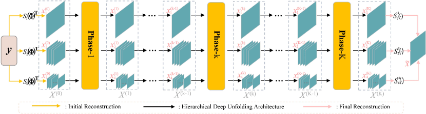
Figure 1. Diagram of the proposed FHDUN, which consists of multiple phases to gradually reconstruct the target image. In FHDUN, series of branches of different scales are included to form a hierarchical structure.

The main contributions are summarized as follows:

(1) A novel Fast Hierarchical Deep Unfolding Network (FHDUN) for image CS is proposed, which can cooperatively infer the optimization solver FISTA in multi-scale spaces to explore richer contextual prior information.

(2) In our framework, series of hyperparametric generation networks are designed to dynamically generate the optimal hyperparameters according to the input content, which greatly enhances the adaptability of the proposed model.

(3) Due to the introduction of the acceleration policy by unfolding the traditional FISTA, the proposed FHDUN is able to save more than 50% of the iterative loops compared with the recent deep unfolding CS networks.

(4) Extensive experiments show that the proposed FHDUN outperforms existing state-of-the-art CS reconstruction networks by large margins with fewer iterations.

2. Related Work

2.1. Uninterpretable DBN

Deep black box network (DBN) usually directly builds an inverse deep mapping from the measurement domain to the original image domain. Due to its simplicity, this kind of method is widely favored by many researchers. Specifically, the early works(Kulkarni et al., 2016; Weng et al., 2018; Yao et al., 2019) usually reconstruct the target image block-by-block and then splice the reconstructed image blocks together into a final reconstructed image. However, these block-by-block methods usually suffer from serious block artifacts(Cui et al., 2018). To relieve this problem, several literatures(Shi et al., 2019, 2020, 2017; Sun et al., 2020a) attempt to explore the deep image priors in the whole image space. Specifically, these CS methods still adopt the block-based sampling(Gan, 2007), however during the reconstruction, they first concatenate all image blocks together in the initial reconstruction, and then complete a deep reconstruction in the whole image space. More recently, to enhance the applicability of CS framework, several scalable CS networks(Shi et al., 2019; Xu et al., 2018) are proposed, which achieve scalable sampling and reconstruction with only one model.

Compared with the traditional optimization-based CS methods, the aforementioned deep black box CS networks can automatically explore image priors on massive training data and achieve higher reconstruction performance with fast computational speed. However, these CS networks usually train the deep network as a black box, which makes these methods lack essential theoretical basis and interpretability, thus limiting the reconstructed quality significantly.

2.2. Interpretable DUN

Deep unfolding network (DUN) usually unfolds certain optimization algorithms into deep network forms to enjoy a better interpretability, which has been applied to solve diverse low-level vision problems, such as denoising(Lefkimmiatis, 2017), debluring(Kruse et al., 2017), and demosaicking (Kokkinos and Lefkimmiatis, 2018). Recently, considering CS reconstruction, some DUNs attempt to integrate some effective convolutional neural networks with some optimization methods including half quadratic splitting (HQS)(Aggarwal et al., 2019; Zhang et al., 2017), alternating minimization, approximate message passing (AMP)(Zhang et al., 2021; Zhou et al., 2020) and alternating direction method of multipliers (ADMM)(Yang et al., 2020). As above, different optimization algorithms usually lead to different optimization-inspired DUNs.

Iterative shrinkage-shresholding algorithm (ISTA)(Beck and Teboulle, 2009), as a prevailing optimization method, has been widely used to solve many large-scale linear inverse problems. To solve Eq.(1), each iteration of ISTA involves gradient descent updating followed by a proximal operator:

(2) $$x^{(k)}=\mathcal{H}(x^{(k-1)}-\rho\Phi^{\rm T}(\Phi x^{(k-1)}-y))\vspace{-0.02in}$$

where $\rho$ is the step size for gradient descent updating and $\mathcal{H}$ indicates a specific shrinkage/soft-threshold function (i.e., proximal operator). Recently, several excellent DUNs attempt to embed deep networks into ISTA to solve CS problem by iterating between the following update steps:

(3) $$r^{(k)}=x^{(k-1)}-\rho^{(k)}\Phi^{\rm T}(\Phi x^{(k-1)}-y)$$

(4) $$x^{(k)}=\mathcal{H}_{\psi}^{(k)}(r^{(k)})$$

where Eq.(3) is responsible for the gradient descent of linear projection and $\rho^{(k)}$ is a learnable step size. Eq.(4) corresponds to a specific proximal operator, which is usually fitted by series of convolutional layers to learn a deep proximal mapping. $\mathcal{H}_{\psi}^{(k)}$ signifies the embedded deep network for exploring the image prior $\psi$. Based on Eqs.(3) and (4), several ISTA-inspired CS DUNs(Zhang and Ghanem, 2018; Zhang et al., 2020; Song et al., 2021; You et al., 2021) have been proposed to reconstruct the target image from measurements.

Apparently, compared with deep black box CS network, the aforementioned deep unfolding CS networks have better interpretability. However, these algorithms usually adopt a plain network architecture and therefore cannot fully exert the expressiveness of the proposed model for image reconstruction. Besides, due to the absence of the acceleration strategy in recent DUNs, the convergence usually requires dozens of iterations, for example MADUN(Song et al., 2021) and COAST(You et al., 2021) respectively need 25 and 20 iterations, which limits their practical applications in some real-time CS systems.

3. Proposed Method

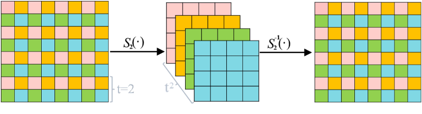
Figure 2. The operation details of the introduced unshuffle operator $S_{t}$ and its inverse operator $S_{t}^{-1}$ under the condition of scale factor $t$$=$2.

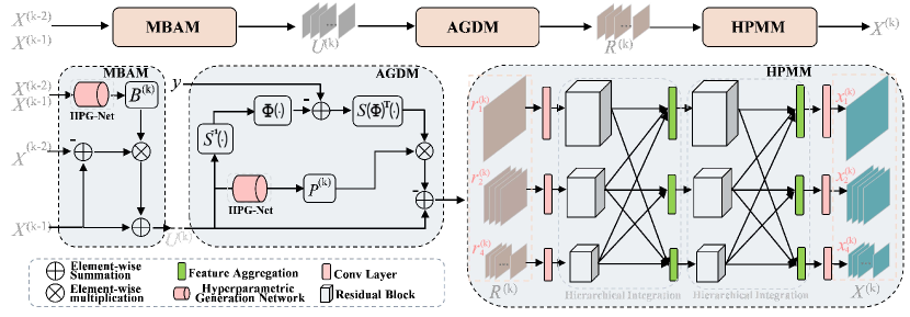
Figure 3. The network in each phase, which includes three modules: Momentum Based Acceleration Module (MBAM), Adaptive Gradient Descent Module (AGDM), Hierarchical Proximal Mapping Module (HPMM).

3.1. Preliminary

As described in Subsection 2.2, ISTA provides rich theoretical inspirations for many recent deep unfolding CS networks. However, ISTA is generally recognized as a time-consuming method because of its requirement for tedious repeated iterations. To alleviate this problem, two fast versions of ISTA are proposed, including the two-step IST (TwIST) algorithm(Bioucas-Dias and Figueiredo, 2007) and fast IST algorithm (FISTA)(Beck and Teboulle, 2009). By embedding the momentum-based acceleration method into ISTA, FISTA solves Eq.(1) by iterating the following update steps:

(5) $$t^{(k)}=\frac{1+\sqrt{1+4(t^{(k-1)})^{2}}}{2}$$

(6) $$u^{(k)}=x^{(k-1)}+(\frac{t^{(k-1)}-1}{t^{(k)}})(x^{(k-1)}-x^{(k-2)})$$

(7) $$x^{(k)}=\mathcal{H}(u^{(k)}-\rho\Phi^{\rm T}(\Phi u^{(k)}-y))$$

Compared with ISTA solver as shown in Eq.(2), the main improvement of FISTA is that the proximal operator $\mathcal{H}$ is not applied on the previous estimation $x_{(k-1)}$, but rather at $u_{(k)}$ which adopts a well-designed linear combination of the previous two estimations $x_{(k-1)}$ and $x_{(k-2)}$.

According to Eqs.(5)-(7), FISTA can be appropriately unfolded into the following iterative update steps:

(8) $$u^{(k)}=x^{(k-1)}+\beta^{(k)}(x^{(k-1)}-x^{(k-2)})$$

(9) $$r^{(k)}=u^{(k)}-\rho^{(k)}\Phi^{\rm T}(\Phi u^{(k)}-y)$$

(10) $$x^{(k)}=\mathcal{H}_{\psi}^{(k)}(r^{(k)})$$

where Eq.(8) is mainly responsible for acceleration by computing a new intermediate variable from $x_{(k-1)}$ and $x_{(k-2)}$, and $\beta^{(k)}$ represents the scalar for momentum update. Eqs.(9) and (10) have the same meaning as Eqs.(3) and (4), which respectively signify gradient descent and proximal mapping.

3.2. Overview of FHDUN

It is clear from Eqs.(8)-(10) that the variable $x^{(k)}$ bridges the gap between different iterations, and a rough $x^{(k)}$ usually hinders information transmission between adjacent iterations, thus losing much more image details during reconstruction. Based on above, we propose a novel hierarchical unfolding architecture (in Fig.1), which consists of multiple branches of different scales that form a hierarchical structure.

In order to build the hierarchical model integrating multiple scales, we first introduce a series of unshuffle operators $\{S_{t}\}$, which approximately can be regarded as the inverse operation of PixelShuffle (widely used in super-resolution tasks)(Shi et al., 2016), and $t$ has a similar meaning to the scale factor in PixelShuffle. Given $\{S_{t}\}$, we use $\{S^{-1}_{t}\}$ to represent their corresponding inverse operations. Fig.2 shows more details of the operators $S_{t}$ and $S^{-1}_{t}$ under the condition of $t$=2. As above, the update steps of Eqs.(8)-(10) in a specific scale space can be intuitively expressed as:

(11) $$u_{t}^{(k)}=x_{t}^{(k-1)}+\beta_{t}^{(k)}(x_{t}^{(k-1)}-x_{t}^{(k-2)})$$

(12) $$r_{t}^{(k)}=u_{t}^{(k)}-\rho_{t}^{(k)}S_{t}(\Phi)^{\rm T}(\Phi S_{t}^{-1}(u_{t}^{(k)})-y)$$

(13) $$x_{t}^{(k)}=\mathcal{H}_{\psi_{t}}^{(k)}(r_{t}^{(k)})$$

where $x_{t}^{(k-1)}$, $x_{t}^{(k-2)}$, $u_{t}^{(k)}$, $r_{t}^{(k)}$ and $x_{t}^{(k)}$ are the variables under the scale factor of $t$. $\beta_{t}^{(k)}$ and $\rho_{t}^{(k)}$ are the corresponding learnable parameters. $\mathcal{H}_{\psi_{t}}^{(k)}$ indicates a deep neural network (proximal mapping) in current scale space (scale factor is $t$) to explore the prior knowledge $\psi_{t}$.

In order to collaboratively integrate the update steps (i.e., Eqs.(11)-(13)) in different scale spaces, we attempt to aggregate the unfolding models of different scales together and propose a novel hierarchical unfolding architecture:

(14) $$U^{(k)}=X^{(k-1)}+B^{(k)}(X^{(k-1)}-X^{(k-2)})$$

(15) $$R^{(k)}=U^{(k)}-P^{(k)}S(\Phi)^{\rm T}(\Phi S^{-1}(U^{(k)})-y)$$

(16) $$X^{(k)}=\mathcal{H}_{\Psi}^{(k)}(R^{(k)})$$

where $X^{(k-1)}$, $X^{(k-2)}$, $U^{(k)}$, $R^{(k)}$ and $X^{(k)}$ are variable sets. For example, $X^{(k)}$=$\{x_{t}^{(k)}\}$, and $t=\{1,2,...\}$. $B^{(k)}$ and $P^{(k)}$ are learnable parameter sets. Analogously, $S(\cdot)$ and $S^{-1}(\cdot)$ respectively signify the collections of the unshuffle operators and their inverse versions under multiple scale spaces. $\mathcal{H}_{\Psi}^{(k)}$ is a unified deep neural network (proximal mapping) to explore the priors $\Psi$ in multiple scale spaces. It is noted that compared with $\psi$ and $\psi_{t}$, $\Psi$ represents more sophisticated priors, including the image priors in each scale space, the correlation priors among different scale spaces and so on.

For the initial reconstruction of our FHDUN, we set $X^{(0)}$= $S(\Phi)^{\rm T}y$, after which the update steps as shown in Eqs.(14)-(16) are iteratively performed. Finally, we average the outputs of different branches to obtain the final reconstruction $\tilde{x}$.

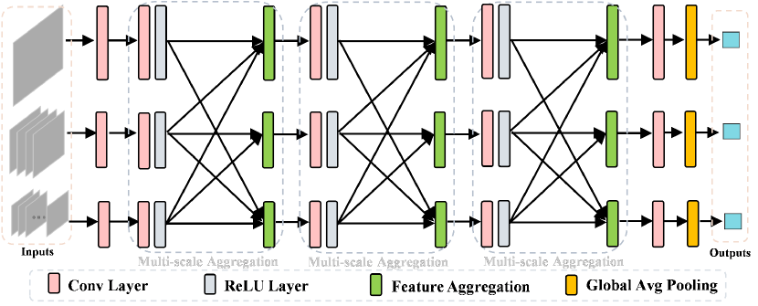
Figure 4. The network structure details of the proposed HPG-Net in MBAM and AGDM. The strcture of feature aggregation is shown in Fig.5(b).

Corresponding to Eqs.(14)-(16), each iteration of our FHDUN consists of three functional modules (in Fig.3): Momentum Based Acceleration Module (MBAM), Adaptive Gradient Descent Module (AGDM) and Hierarchical Proximal Mapping Module (HPMM). The following subsections will describe more details about these three modules.

Table 1. Average PSNR and SSIM comparisons of recent deep network-based CS algorithms using random sampling matrix on dataset Set11. Bold indicates the best result, underline signifies the second best result.

Algorithms	Ratio=0.01		Ratio=0.10		Ratio=0.25		Ratio=0.30		Ratio=0.40		Avg.
	PSNR	SSIM	PSNR	SSIM	PSNR	SSIM	PSNR	SSIM	PSNR	SSIM	PSNR	SSIM
ReconNet(Kulkarni et al., 2016)	17.54	0.4426	24.07	0.6958	26.38	0.7883	28.72	0.8517	30.59	0.8928	25.46	0.7342
I-Recon(Weng et al., 2018)	19.80	0.5018	25.97	0.7888	28.52	0.8547	31.45	0.9135	32.26	0.9243	27.60	0.7966
DR2-Net(Yao et al., 2019)	17.44	0.4294	24.71	0.7175	– –	– –	30.52	– –	31.20	– –	– –	– –
DPA-Net(Sun et al., 2020a)	18.05	0.5011	26.99	0.8354	32.38	0.9311	33.35	0.9425	35.21	0.9580	29.20	0.8336
IRCNN(Zhang et al., 2017)	7.70	0.3324	23.05	0.6789	28.42	0.8382	29.55	0.8606	31.30	0.8898	24.00	0.7200
LDAMP(Metzler et al., 2017)	17.51	0.4409	24.94	0.7483	– –	– –	32.01	0.9144	34.07	0.9393	– –	– –
ISTA-Net+(Zhang and Ghanem, 2018)	17.45	0.4131	26.49	0.8036	32.48	0.9242	33.81	0.9393	36.02	0.9579	29.25	0.8076
DPDNN(Dong et al., 2019)	17.59	0.4459	26.23	0.7992	31.71	0.9153	33.16	0.9338	35.29	0.9534	28.80	0.8095
NN(Gilton et al., 2020)	17.67	0.4324	23.90	0.6927	29.20	0.8600	30.26	0.8833	32.31	0.9137	26.67	0.7564
MAC-Net(Chen et al., 2020)	18.26	0.4566	27.68	0.8182	32.91	0.9244	33.96	0.9372	36.18	0.9562	29.80	0.8185
iPiano-Net(Su and Lian, 2020)	19.38	0.4812	28.05	0.8460	33.53	0.9359	34.78	0.9472	37.00	0.9631	30.55	0.8347
FHDUN	20.18	0.5468	29.53	0.8859	35.01	0.9512	36.12	0.9589	38.04	0.9696	31.78	0.8625

3.3. MBAM for Fast Convergence

From Eq.(14), the mission of MBAM is to accelerate the convergence by computing a new variable set $U^{(k)}$ from $X^{(k-1)}$ and $X^{(k-2)}$. Apparently, the momentum scalar $B^{(k)}$ has a crucial influence on the convergence efficiency of the proposed model. Different from the existing hyperparametric learning strategies (once the training is completed, the learned hyperparameters are fixed for any input content), a novel hyperparametric generation network (HPG-Net) as shown in Fig.4 is designed in our framework to dynamically learn the momentum scalar $B^{(k)}$ from the previous iterations:

(17) $$B^{(k)}=\{\beta_{t}^{(k)}\}=F_{(\theta_{u}^{k})}(X^{(k-1)},X^{(k-2)})\vspace{-0.0in}$$

where $F_{(\theta_{u}^{k})}$ indicates the proposed HPG-Net in the current iteration with the learnable parameter $\theta_{u}^{k}$, and its input is the concatenated mixture of $X^{(k-1)}$ and $X^{(k-2)}$. Due to the hierarchical structure of the proposed framework, the developed HPG-Net is able to hierarchically integrate the multi-scale information from different branches. Specifically, three multi-scale aggregation submodules (shown in gray dashed boxes of Fig.4) are introduced in HPG-Net, which can cooperatively explore more information from different scale spaces. After the aggregation submodules, series of convolutional layers and global average pooling layers are appended to generate the final momentum scalars.

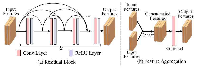
Figure 5. The network structure details of the residual block (a) and the feature aggregation (b).

3.4. AGDM for Gradient Descent

In Eq.(15), AGDM performs the gradient descent for the linear projection. Similar to $B^{(k)}$ (in Eq.(14)), the step size $P^{(k)}$ is also a crucial hyper-parameter that controls the magnitude of the gradient updating. According to Eqs.(3) and (4), the existing ISTA-inspired DUNs directly optimize the step size value from the training data, and once the training is completed, the step size of these methods is fixed for any input content. In our framework, similar to the learning strategy of momentum scalar $B^{(k)}$ (Subsection 3.3), another novel hyperparametric generation network (HPG-Net) is designed (also shown in Fig.4) to adaptively learn the corresponding optimal step size for the given input content:

(18) $$P^{(k)}=\{\rho_{t}^{(k)}\}=J_{(\theta_{r}^{k})}(U^{(k)})\vspace{-0.0in}$$

where $J_{(\theta_{r}^{k})}$ indicates the network HPG-Net in current iteration with the learnable parameter $\theta_{r}^{k}$, and its input is the intermediate variable set $U^{(k)}$ from Eq.(14). It is noted that the proposed HPG-Net in AGDM has the similar network structure with that of MBAM, which can efficiently integrate the multi-scale information from different branches. For more details of HPG-Net, the multi-scale aggregation submodules (gray dashed boxes of Fig.4) are still retained, which can cooperatively explore more information from multiple scale spaces. Finally, series of convolutional layers (with single kernel) and global average pooling layers are appended to generate the final step sizes for different branches.

3.5. HPMM for Proximal Mapping

After gradient descent, the module HPMM corresponding to Eq.(16) is appended, which actually is a deep convolutional neural network (dubbed HPM-Net) in our framework. For more details of the proposed HPM-Net, a series of horizontal branches are included as shown in Fig.3 to form a hierarchical structure. Specifically, the horizontal branch is responsible for the feature extraction under a certain scale space. The transformations among different scales are performed between all the horizontal branches, including both downsampling and upsampling operations. For more internal details, two hierarchical aggregation submodules (the gray dashed boxes of HPMM in Fig.3) are introduced, in which series of residual blocks (Fig.5(a)) and feature aggregation submodules (Fig.5(b)) are utilized to capture and aggregate the deep features of different scales. For simplicity, the learnable parameter in HMP-Net of current iteration is represented as $\theta_{x}^{k}$, which will be utilized in the following sections.

Compared with the proximal mapping of existing DUNs (usually adopt a plain convolutional network to explore image priors at a single scale space), the proposed hierarchical network can cooperatively perceive wider contextual prior information in multi-scale spaces. In addition, due to the hierarchical architecture design, the proposed DUN can persist and transmit more richer information between neighbouring iterations for boosting reconstructed quality.

Table 2. Average PSNR and SSIM comparisons of recent deep network-based CS algorithms using learned sampling matrix on dataset Set5. Bold indicates the best result, and underline signifies the second best result.

Algorithms	Ratio=0.01		Ratio=0.10		Ratio=0.25		Ratio=0.30		Ratio=0.40		Avg.
	PSNR	SSIM	PSNR	SSIM	PSNR	SSIM	PSNR	SSIM	PSNR	SSIM	PSNR	SSIM
CSNet${\rm{\color[rgb]{0,0,1}(ICME2017)}}$(Shi et al., 2017)	24.02	0.6378	32.30	0.9015	36.63	0.9562	37.90	0.9630	39.89	0.9736	34.15	0.8864
LapCSNet${\rm{\color[rgb]{0,0,1}(ICASSP2018)}}$(Cui et al., 2018)	24.42	0.6686	32.44	0.9047	– –	– –	– –	– –	– –	– –	– –	– –
SCSNet${\rm{\color[rgb]{0,0,1}(CVPR2019)}}$(Shi et al., 2019)	24.21	0.6468	32.77	0.9083	37.20	0.9558	38.45	0.9655	40.44	0.9755	34.61	0.8904
CSNet+${\rm{\color[rgb]{0,0,1}(TIP2020)}}$(Shi et al., 2020)	24.18	0.6478	32.59	0.9062	37.11	0.9560	38.25	0.9644	40.11	0.9740	34.45	0.8897
NL-CSNet${\rm{\color[rgb]{0,0,1}(TMM2021)}}$(Cui et al., 2021)	24.82	0.6771	33.84	0.9312	37.78	0.9635	38.86	0.9703	40.69	0.9778	35.20	0.9040
BCS-Net${\rm{\color[rgb]{0,0,1}(TMM2020)}}$(Zhou et al., 2020)	22.98	0.6103	32.71	0.9030	37.90	0.9576	38.64	0.9694	39.88	0.9785	34.42	0.8838
OPINENet+${\rm{\color[rgb]{0,0,1}(JSTSP2020)}}$(Zhang et al., 2020)	22.76	0.6194	33.72	0.9259	38.05	0.9631	39.14	0.9689	41.07	0.9780	34.95	0.8911
AMP-Net+${\rm{\color[rgb]{0,0,1}(TIP2021)}}$(Zhang et al., 2021)	23.00	0.6488	33.35	0.9162	38.00	0.9606	39.07	0.9671	40.94	0.9765	34.87	0.8938
COAST${\rm{\color[rgb]{0,0,1}(TIP2021)}}$(You et al., 2021)	23.31	0.6514	33.90	0.9266	38.21	0.9648	39.23	0.9706	41.36	0.9780	35.20	0.8983
MADUN${\rm{\color[rgb]{0,0,1}(ACMMM2021)}}$(Song et al., 2021)	23.12	0.6503	33.86	0.9267	38.44	0.9660	39.57	0.9723	41.72	0.9808	35.34	0.8992
FHDUN	24.04	0.6705	34.25	0.9345	38.78	0.9682	39.90	0.9734	41.98	0.9812	35.79	0.9056

Table 3. Average PSNR and SSIM comparisons of recent deep network-based CS algorithms using learned sampling matrix on dataset Set14. Bold indicates the best result, underline signifies the second best result.

Algorithms	Ratio=0.01		Ratio=0.10		Ratio=0.25		Ratio=0.30		Ratio=0.40		Avg.
	PSNR	SSIM	PSNR	SSIM	PSNR	SSIM	PSNR	SSIM	PSNR	SSIM	PSNR	SSIM
CSNet${\rm{\color[rgb]{0,0,1}(ICME2017)}}$ (Shi et al., 2017)	22.79	0.5628	28.91	0.8119	32.86	0.9057	34.00	0.9276	35.84	0.9481	30.88	0.8312
LapCSNet${\rm{\color[rgb]{0,0,1}(ICASSP2018)}}$(Cui et al., 2018)	23.16	0.5818	29.00	0.8147	– –	– –	– –	– –	– –	– –	– –	– –
SCSNet${\rm{\color[rgb]{0,0,1}(CVPR2019)}}$(Shi et al., 2019)	22.87	0.5631	29.22	0.8181	33.24	0.9073	34.51	0.9311	36.54	0.9525	31.28	0.8344
CSNet+${\rm{\color[rgb]{0,0,1}(TIP2020)}}$(Shi et al., 2020)	22.83	0.5630	29.13	0.8169	33.19	0.9064	34.34	0.9297	36.16	0.9502	31.13	0.8332
NL-CSNet${\rm{\color[rgb]{0,0,1}(TMM2021)}}$(Cui et al., 2021)	23.61	0.5862	30.16	0.8527	33.84	0.9270	34.88	0.9405	36.86	0.9573	31.87	0.8527
BCS-Net${\rm{\color[rgb]{0,0,1}(TMM2020)}}$(Zhou et al., 2020)	22.38	0.5543	29.73	0.8384	34.50	0.9279	35.53	0.9390	37.46	0.9537	31.92	0.8427
OPINENet+${\rm{\color[rgb]{0,0,1}(JSTSP2020)}}$(Zhang et al., 2020)	22.30	0.5508	29.94	0.8415	34.31	0.9268	35.18	0.9369	37.51	0.9572	31.85	0.8426
AMP-Net+${\rm{\color[rgb]{0,0,1}(TIP2021)}}$(Zhang et al., 2021)	22.60	0.5723	29.87	0.8130	34.27	0.9218	35.23	0.9364	37.42	0.9561	31.88	0.8399
COAST${\rm{\color[rgb]{0,0,1}(TIP2021)}}$(You et al., 2021)	22.81	0.5764	30.26	0.8507	34.72	0.9335	35.66	0.9404	37.86	0.9598	32.26	0.8522
MADUN${\rm{\color[rgb]{0,0,1}(ACMMM2021)}}$(Song et al., 2021)	22.44	0.5675	30.17	0.8483	34.98	0.9362	36.03	0.9473	38.27	0.9641	32.38	0.8527
FHDUN	23.23	0.5906	30.76	0.8596	35.32	0.9381	36.41	0.9489	38.55	0.9645	32.85	0.8603

4. Experiments and Analysis

4.1. Loss Function

Given the full-sampled image $x_{i}$ and the sampling matrix $\Phi$, the compressed measurements can be obtained by $y_{i}=\Phi x_{i}$. Our proposed FHDUN takes $y_{i}$ and $\Phi$ as inputs and aims to narrow down the gap between the output and the target image $x_{i}$. Since the proposed FHDUN consists of multiple phases, series of outputs $\{(x_{i})_{t}^{k}\}$ are generated through the pipeline of the entire framework, where $t$ represents the scale factor in the hierarchical structure, and $k$ is the index of the phase number in the proposed CS framework.

In our proposed FHDUN, the outputs of different scales in all phases are constrained. Specifically, we directly use the L2 norm to restrain the distance between the outputs $(x_{i})_{t}^{k}$ and the corresponding real entities $S_{t}(x_{i})$, i.e.,

(19) $$\mathcal{L}(\Theta)=\frac{1}{KN_{a}}\sum_{i=1}^{N_{a}}\sum_{k=1}^{K}\sum_{t\in T}||(x_{i})_{t}^{k}-S_{t}(x_{i})||_{F}^{2}$$

where $\Theta$ denotes the learnable parameter set of our proposed FHDUN, including $\{\theta_{u}^{k}\}$ in MBAM, $\{\theta_{r}^{k}\}$ in AGDM and $\{\theta_{x}^{k}\}$ in HPMM. It worth noting that since multiple entities of different scales are revealed during the network execution, we use $S_{t}(x_{i})$, rather than $x_{i}$, as the corresponding label. In addition, $N_{a}$, $T$ and $K$ represent the number of training images, scale factor set in the hierarchical structure and the phase number of our FHDUN respectively.

4.2. Implementation and Training Details

In the proposed CS framework, we set the scale factor set $T$=$\{1,2,4\}$, that is to say, the proposed hierarchical framework consists of three horizontal branches of different scales (as shown in Fig.1). Considering the phase number $K$, Fig.6 shows the relationship between the phase number and the reconstructed quality, and we set $K$=8 in our model, which saves more than 50% iteration loops against recent DUNs (such as MADUN(Song et al., 2021) and COAST(You et al., 2021)). For more configuration details of networks HPG-Net and HPM-Net in our framework, the channel numbers of the intermediate feature maps in their three horizontal branches are respectively set as 16, 32 and 64. In the residual blocks of HPM-Net, the number of convolutional layer is set as $d$=3. In addition, with the exception of the convolutional layer in the feature aggregation submodule (in Fig.5(b)), which has the convolutional kernel size of 1$\times$1, the kernel size of all other convolutional layers is set to 3$\times$3. We initialize the convolutional filters using the same method as(He et al., 2015) and pad zeros around the boundaries to keep the size of all feature maps.

Table 4. Average PSNR and SSIM comparisons of recent deep unfolding CS networks using learned sampling matrix on dataset BSD68. Bold indicates the best result, underline signifies the second best result.

Algorithms	Ratio=0.01		Ratio=0.10		Ratio=0.25		Ratio=0.30		Ratio=0.40		Avg.
	PSNR	SSIM	PSNR	SSIM	PSNR	SSIM	PSNR	SSIM	PSNR	SSIM	PSNR	SSIM
BCS-Net${\rm{\color[rgb]{0,0,1}(TMM2020)}}$(Zhou et al., 2020)	22.16	0.5287	27.78	0.7864	31.14	0.9006	32.15	0.9167	33.90	0.9473	29.43	0.8159
OPINENet+${\rm{\color[rgb]{0,0,1}(JSTSP2020)}}$(Zhang et al., 2020)	21.88	0.5162	27.81	0.8040	31.50	0.9062	32.78	0.9278	34.73	0.9521	29.74	0.8213
AMP-Net+${\rm{\color[rgb]{0,0,1}(TIP2021)}}$(Zhang et al., 2021)	21.94	0.5253	27.86	0.7928	31.75	0.9050	32.84	0.9242	34.86	0.9509	29.85	0.8196
COAST${\rm{\color[rgb]{0,0,1}(TIP2021)}}$(You et al., 2021)	22.30	0.5391	27.80	0.8091	31.81	0.9128	32.78	0.9331	34.90	0.9565	29.92	0.8301
MADUN${\rm{\color[rgb]{0,0,1}(ACMMM2021)}}$(Song et al., 2021)	21.65	0.5249	27.74	0.8108	31.90	0.9165	32.96	0.9353	35.02	0.9584	29.86	0.8293
FHDUN	22.58	0.5395	28.29	0.8173	32.16	0.9189	33.24	0.9360	35.33	0.9589	30.32	0.8341

Table 5. Average PSNR and SSIM comparisons of recent deep unfolding CS networks using learned sampling matrix on dataset Urban100. Bold indicates the best result, underline signifies the second best result.

Algorithms	Ratio=0.01		Ratio=0.10		Ratio=0.25		Ratio=0.30		Ratio=0.40		Avg.
	PSNR	SSIM	PSNR	SSIM	PSNR	SSIM	PSNR	SSIM	PSNR	SSIM	PSNR	SSIM
BCS-Net${\rm{\color[rgb]{0,0,1}(TMM2020)}}$(Zhou et al., 2020)	20.64	0.5148	28.26	0.8469	33.52	0.9348	34.51	0.9532	36.76	0.9680	30.74	0.8435
OPINENet+${\rm{\color[rgb]{0,0,1}(JSTSP2020)}}$(Zhang et al., 2020)	20.56	0.5140	28.84	0.8675	33.77	0.9424	34.91	0.9557	36.98	0.9708	31.01	0.8502
AMP-Net+${\rm{\color[rgb]{0,0,1}(TIP2021)}}$(Zhang et al., 2021)	20.94	0.5386	28.80	0.8589	33.76	0.9383	34.88	0.9546	36.92	0.9701	31.06	0.8521
COAST${\rm{\color[rgb]{0,0,1}(TIP2021)}}$(You et al., 2021)	20.76	0.5279	28.82	0.8690	33.81	0.9452	34.96	0.9573	37.10	0.9712	31.09	0.8540
MADUN${\rm{\color[rgb]{0,0,1}(ACMMM2021)}}$(Song et al., 2021)	20.43	0.5250	28.86	0.8692	33.98	0.9467	35.20	0.9588	37.35	0.9723	31.17	0.8544
FHDUN	21.18	0.5434	29.20	0.8763	34.25	0.9486	35.48	0.9597	37.55	0.9726	31.53	0.8601

We use the training set (400 images) from the BSD500(Arbelaez et al., 2011) dataset as our training data. Furthermore, we augment the training data in the following two ways: ($1$) Rotate the images by 90^∘, 180^∘ and 270^∘ randomly. ($2$) Flip the images horizontally with a probability of 0.5. In the training process, we set block size as 32, i.e., $N$=1024, and in order to alleviate blocking artifacts, we randomly crop the size of patches to 96$\times$96. More specifically, we first unfold the blocks of size 96$\times$96 into non-overlapping blocks of size 32$\times$32 in the sampling process and then concatenate all the blocks together in the initial reconstruction. We also unfold the whole testing image with this approach during testing process. We use the PyTorch toolbox and train our model using the Adaptive moment estimation (Adam) solver on a NVIDIA GTX 3090 GPU. Furthermore, we set the momentum to 0.9 and the weight decay to 1e-4. The learning rate is initialized to 1e-4 for all layers and decreased by a factor of 2 for every 30 epochs. We train our model for 200 epochs totally and 1000 iterations are performed for each epoch. Therefore, 200$\times$1000 iterations are completed in the whole training process.

4.3. Comparisons with Other Methods

Depending on whether the sampling matrix $\Phi$ can be learned jointly with the reconstruction process, we conduct two types of experimental comparisons: comparisons with the random sampling matrix-based CS methods and the learned sampling matrix-based CS methods. For testing data, we carry out extensive experiments on several representative benchmark datasets: Set5(Shi et al., 2019), Set14(Cui et al., 2018), Set11(Chen et al., 2020), BSD68(Sun et al., 2020a) and Urban100(Song et al., 2021), which are widely used in the recent CS-related works. To ensure the fairness, we evaluate the reconstruction performance with two widely used quality evaluation metrics: PSNR and SSIM in terms of various sampling ratios.

Random Sampling Matrix: For the random sampling matrix-based CS methods, we compare our proposed FHDUN with eleven recent representative deep network-based reconstruction algorithms, including four deep black box networks (ReconNet(Kulkarni et al., 2016), I-Recon(Weng et al., 2018), DR²-Net(Yao et al., 2017) and DPA-Net(Sun et al., 2020a)) and seven DUNs (IRCNN(Zhang et al., 2017), LD-AMP (Metzler et al., 2017), ISTA-Net⁺(Zhang and Ghanem, 2018), DPDNN(Dong et al., 2019), NN(Gilton et al., 2020), MAC-Net(Chen et al., 2020) and iPiano-Net(Su and Lian, 2020)). For these compared methods, we train them with the same experimental configurations as(Song et al., 2021). In our FHDUN, the orthogonalized Gaussian random matrix(Sun et al., 2020a, b) is utilized. Table 1 presents the average PSNR and SSIM comparisons at five sampling ratios (i.e., 0.01, 0.10, 0.25, 0.30, 0.40) on dataset Set11, from which we can observe that the proposed FHDUN outperforms all the compared methods in PSNR and SSIM by large margins.

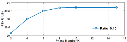
Figure 6. The relationship between the phase number and the image quality (PSNR) on dataset Set11.

Learned Sampling Matrix: For the learned sampling matrix-based CS methods, the sampling matrix is jointly optimized with the reconstruction module, which facilitates the collaborations between the sampling and reconstruction. For comparative fairness, ten recent deep network-based literatures, i.e., CSNet(Shi et al., 2017), LapCSNet(Cui et al., 2018), SCSNet(Shi et al., 2019), CSNet⁺(Shi et al., 2020), NL-CSNet(Cui et al., 2021), BCS-Net(Zhou et al., 2020), OPINE-Net (Zhang et al., 2020), AMP-Net(Zhang et al., 2021), COAST(You et al., 2021) and MADUN(Song et al., 2021) participate in the comparison in our experiments, and the first five algorithms are the black box CS networks, the last five schemes belong to the deep unfolding models. For these compared methods, we obtain the experimental results by running their published source codes. Tables 2,3 present the experimental comparisons at the given five sampling ratios on dataset Set5 and Set14, from which we can observe that the proposed FHDUN performs much better than the other deep network-based CS schemes. To further evaluate the performance of our proposed FHDUN, we conduct more comparisons compared with recent CS DUNs on two benchmark datasets BSD68 and Urban100, and the results are shown in Tables 4, 5. Compared with the recent MADUN, the proposed FHDUN can achieve on average 0.93dB, 0.55dB, 0.26dB, 0. 28dB, 0.31dB gains on dataset BSD68. For dataset Urban100, the proposed FHDUN achieves on average 0.75dB, 0.34dB, 0.27dB, 0.28dB, 0.20dB gains in PSNR compared with MADUN. The visual comparisons are shown in Fig. 7, from which we observe that the proposed method can preserve more details and retain sharper edges compared to the other CS networks.

Table 6. The ablation results of the proposed FHDUN on dataset Set14.

MBAM	AGDM	HPMM	0.10	0.25	0.30	0.40
✗	✓	✓	30.59	35.22	36.24	38.42
$\checkmark$	✗	$\checkmark$	30.51	35.09	36.16	38.28
$\checkmark$	$\checkmark$	✗	30.18	34.68	35.95	38.17
✓	$\checkmark$	$\checkmark$	30.76	35.32	36.41	38.55

GT$\backslash$PSNR$\backslash$SSIM

NLCSNet$\backslash$35.44$\backslash$0.9098

OPINE$\backslash$35.24$\backslash$0.9021

AMPNet$\backslash$34.85$\backslash$0.8900

COAST$\backslash$35.60$\backslash$0.9104

MADUN$\backslash$35.58$\backslash$0.9114

Ours$\backslash$36.15$\backslash$0.9210

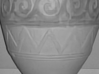
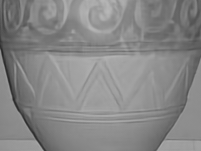
Figure 7. Visual quality comparisons between the proposed FHDUN and recent deep network-based CS methods that use learned sampling matrix on one testing image sample from BSD68 at sampling ratio of 0.10.

From Tables 2,3, we observe that NL-CSNet(Cui et al., 2021) outperforms FHDUN at lowest sampling rate of 0.01. A reasonable explanation is provided bellow. NL-CSNet is a deep black box CS network, which directly build an inverse deep mapping from the measurement domain to the image domain. Different from DUNs, the sampling matrix of NL-CSNet is not well embedded into its reconstruction process, which leads to the sampling matrix cannot provide the necessary guidance for the image reconstruction, thus making the reconstructed performance of(Cui et al., 2021) seriously depends on the network structure design and its careful tuning strategy. Apparently, with the increase of sampling ratio, the dimension of sampling matrix is higher, which can provide more guidance for the reconstruction. Therefore, with the sampling ratio increases, the proposed FHDUN achieves much better reconstruction performance against NL-CSNet. Specifically, on the one hand, when sampling ratio is very low (such as 0.01), the guidance provided by the sampling matrix is very limited, and the reconstruction performance mainly comes from the network design and fine-tuning policy. As above, the complexed network structure of NL-CSNet makes better reconstructed quality compared with our FHDUN at low sampling ratio 0.01. On the other hand, when the sampling ratio becomes larger, the sampling matrix can provide more guidance, and therefore the proposed FHDUN begins to obtain better reconstruction quality against NL-CSNet. This phenomenon is also reflected in other CS methods as shown in Tables 2,3.

Considering the parameter quantities and running speed. Because MADUN(Song et al., 2021) achieves the best performance in the compared methods, we mainly analyze the comparisons against MADUN. The following analysis is based on the models with the sampling ratio of 0.10. For the number of parameters, the parameter quantities of MADUN and FHDUN respectively are 3.02M and 3.68M. For running speed, we test three images with different resolutions of 256x256, 720x576, 1024x768 in the same platform (GTX 3090 GPU), and the running times (in second) of MADUN and FHDUN are 0.0364, 0.0867, 0.2132 and 0.0349, 0.0786, 0.1980 respectively. As above, due to the hierarchical architecture, the proposed FHUDN has more parameters compared with MADUN. However, because most of the convolutional layers are performed on lower resolution feature maps, the running speed of the proposed FHDUN is competitive with MADUN.

4.4. Ablation Studies

As above, the proposed CS framework achieves higher reconstruction quality. In order to evaluate the contributions of each part of the proposed FHDUN, we design several variations of the proposed model, in which some functional modules are selectively discarded or replaced. Table 6 shows the experimental results on the dataset Set14, in which three functional modules, i.e., MBAM, AGDM and HPMM, are considered. It should be noted that when MBAM or AGDM are discarded, we replace our HPG-Net with the hyperparametric learning method in the existing DUNs(Zhang and Ghanem, 2018; Zhang et al., 2020). Besides, when HPMM is discarded, we only retain the first horizontal branch of the proposed hierarchical architecture for CS reconstruction. The experimental results reveal that the proposed hierarchical network architecture can bring a maximum gain compared with other two modules. As a note, each of these three modules can enhance the CS reconstruction performance to varying degrees.

To further verify the effectiveness of the introduced acceleration module MBAM, a new variant without MBAM module, dubbed FHDUN(w/o-M), is designed. We train this variant from scratch with the same configurations as FHDUN, and we find that the convergence of FHDUN(w/o-M) needs about 15 iterations (testing on dataset Set11 at sampling ratio of 0.10 same as Fig.6). Compared with the recent MADUN(Song et al., 2021) and COAST(You et al., 2021), the variant FHDUN(w/o-M) clearly requires fewer iterations, which may be caused by the newly introduced network components, such as hierarchical architecture and hyperparametric generation network. On the other hand, considering the iterations of FHDUN(w/o-M) and FHDUN, we can get that the introduced acceleration module MBAM can save nearly half of the iterations.

5. Conclusion

In this paper, a novel Fast Hierarchical Deep Unfolding CS Network (FHDUN) based on the traditional solver FISTA is proposed, in which a well-designed hierarchical architecture is developed to cooperatively perceive the richer contextual prior information in multi-scale spaces. Due to the hierarchical design, the proposed framework is able to persist and transmit richer textures and structures among cascading iterations for boosting reconstructed quality. In addition, series of hyperparametric generation networks are developed in our framework to dynamically produce the corresponding hyperparameters according to the input content, which enhances the adaptability of the proposed model. Moreover, by unfolding the traditional FISTA, the newly introduced acceleration module can save more than 50% of the iterative loops against recent DUNs. Extensive CS experiments manifest that the proposed FHDUN outperforms existing state-of-the-art CS methods.

6. ACKNOWLEDGMENTS

This work was supported by the National Natural Science Foundation of China under Grant 61872116.

References

- (1)
- Aggarwal et al. (2019) Hemant K. Aggarwal, Merry P. Mani, and Mathews Jacob. 2019. MoDL: Model-Based Deep Learning Architecture for Inverse Problems. IEEE Transactions on Medical Imaging 38, 2 (2019), 394–405. https://doi.org/10.1109/TMI.2018.2865356
- Anselmi et al. (2015) Nicola Anselmi, Marco Salucci, Giacomo Oliveri, and Andrea Massa. 2015. Wavelet-Based Compressive Imaging of Sparse Targets. IEEE Transactions on Antennas and Propagation 63, 11 (2015), 4889–4900. https://doi.org/10.1109/TAP.2015.2444423
- Arbelaez et al. (2011) Pablo Arbelaez, Michael Maire, Charless Fowlkes, and Jitendra Malik. 2011. Contour detection and hierarchical image segmentation. IEEE Transactions on Pattern Analysis and Machine Intelligence 33, 5 (2011), 898–916.
- Beck and Teboulle (2009) Amir Beck and Marc Teboulle. 2009. A Fast Iterative Shrinkage-Thresholding Algorithm for Linear Inverse Problems. SIAM J. Imaging Sci. 2, 1 (2009), 183–202. https://doi.org/10.1137/080716542
- Bioucas-Dias and Figueiredo (2007) JosÉ M. Bioucas-Dias and MÁrio A. T. Figueiredo. 2007. A New TwIST: Two-Step Iterative Shrinkage/Thresholding Algorithms for Image Restoration. IEEE Transactions on Image Processing 16, 12 (2007), 2992–3004. https://doi.org/10.1109/TIP.2007.909319
- Candes et al. (2006) E. J. Candes, J. Romberg, and T. Tao. 2006. Robust uncertainty principles: exact signal reconstruction from highly incomplete frequency information. IEEE Transactions on Information Theory 52, 2 (2006), 489–509. https://doi.org/10.1109/TIT.2005.862083
- Candès and Wakin (2008) Emmanuel J Candès and Michael B Wakin. 2008. An introduction to compressive sampling. IEEE Signal Processing Magazine 25, 2 (2008), 21–30.
- Chen et al. (2011) C. Chen, E. W. Tramel, and J. E. Fowler. 2011. Compressed-sensing recovery of images and video using multihypothesis predictions. In 2011 Conference Record of the Forty Fifth Asilomar Conference on Signals, Systems and Computers (ASILOMAR). 1193–1198. https://doi.org/10.1109/ACSSC.2011.6190204
- Chen et al. (2020) Jiwei Chen, Yubao Sun, Qingshan Liu, and Rui Huang. 2020. Learning Memory Augmented Cascading Network for Compressed Sensing of Images. In Computer Vision – ECCV 2020, Andrea Vedaldi, Horst Bischof, Thomas Brox, and Jan-Michael Frahm (Eds.). Springer International Publishing, Cham, 513–529.
- Cui et al. (2021) Wenxue Cui, Shaohui Liu, Feng Jiang, and Debin Zhao. 2021. Image Compressed Sensing Using Non-local Neural Network. IEEE Transactions on Multimedia (TMM) (2021). doi:10.1109/TMM.2021.3132489.
- Cui et al. (2018) Wenxue Cui, Heyao Xu, Xinwei Gao, Shengping Zhang, Feng Jiang, and Debin Zhao. 2018. An efficient deep convolutional laplacian pyramid architecture for CS reconstruction at low sampling ratios. IEEE International Conference on Acoustics, Speech and Signal Processing (ICASSP) (2018).
- Dong et al. (2014) W. Dong, G. Shi, X. Li, Y. Ma, and F. Huang. 2014. Compressive Sensing via Nonlocal Low-Rank Regularization. IEEE Transactions on Image Processing 23, 8 (2014), 3618–3632. https://doi.org/10.1109/TIP.2014.2329449
- Dong et al. (2019) W. Dong, P. Wang, W. Yin, G. Shi, F. Wu, and X. Lu. 2019. Denoising Prior Driven Deep Neural Network for Image Restoration. IEEE Transactions on Pattern Analysis and Machine Intelligence 41, 10 (2019), 2305–2318. https://doi.org/10.1109/TPAMI.2018.2873610
- Donoho (2006) David L Donoho. 2006. Compressed sensing. IEEE Transactions on Information Theory 52, 4 (2006), 1289–1306.
- Donoho et al. (2009) David L Donoho, Arian Maleki, and Andrea Montanari. 2009. Message-passing algorithms for compressed sensing. Proceedings of the National Academy of Sciences 106, 45 (2009), 18914–18919.
- Duarte et al. (2008) Marco F. Duarte, Mark A. Davenport, Dharmpal Takhar, Jason N. Laska, Ting Sun, Kevin F. Kelly, and Richard G. Baraniuk. 2008. Single-pixel imaging via compressive sampling. IEEE Signal Processing Magazine 25, 2 (2008), 83–91. https://doi.org/10.1109/MSP.2007.914730
- Gan (2007) Lu Gan. 2007. Block compressed sensing of natural images. Proceedings of the international conference on digital signal processing (2007), 403–406.
- Gao et al. (2015) Xinwei Gao, Jian Zhang, Wenbin Che, Xiaopeng Fan, and Debin Zhao. 2015. Block-based compressive sensing coding of natural images by local structural measurement matrix. IEEE Data Compression Conference (DCC) (2015), 133–142.
- Gilton et al. (2020) D. Gilton, G. Ongie, and R. Willett. 2020. Neumann Networks for Linear Inverse Problems in Imaging. IEEE Transactions on Computational Imaging 6 (2020), 328–343. https://doi.org/10.1109/TCI.2019.2948732
- Golbabaee and Vandergheynst (2012) Mohammad Golbabaee and Pierre Vandergheynst. 2012. Hyperspectral image compressed sensing via low-rank and joint-sparse matrix recovery. In 2012 IEEE International Conference on Acoustics, Speech and Signal Processing (ICASSP). 2741–2744. https://doi.org/10.1109/ICASSP.2012.6288484
- He et al. (2015) Kaiming He, Xiangyu Zhang, Shaoqing Ren, and Jian Sun. 2015. Delving deep into rectifiers: Surpassing human-level performance on imagenet classification. IEEE International Conference on Computer Vision (ICCV) (2015), 1026–1034.
- Kim et al. (2010) Yookyung Kim, Mariappan S. Nadar, and Ali Bilgin. 2010. Compressed sensing using a Gaussian Scale Mixtures model in wavelet domain. In IEEE International Conference on Image Processing(ICIP). 3365–3368.
- Kokkinos and Lefkimmiatis (2018) Filippos Kokkinos and Stamatios Lefkimmiatis. 2018. Deep Image Demosaicking Using a Cascade of Convolutional Residual Denoising Networks. In Computer Vision – ECCV 2018, Vittorio Ferrari, Martial Hebert, Cristian Sminchisescu, and Yair Weiss (Eds.). Springer International Publishing, Cham, 317–333.
- Kruse et al. (2017) Jakob Kruse, Carsten Rother, and Uwe Schmidt. 2017. Learning to Push the Limits of Efficient FFT-Based Image Deconvolution. In 2017 IEEE International Conference on Computer Vision (ICCV). 4596–4604. https://doi.org/10.1109/ICCV.2017.491
- Kulkarni et al. (2016) K. Kulkarni, S. Lohit, P. Turaga, R. Kerviche, and A. Ashok. 2016. ReconNet: Non-Iterative Reconstruction of Images from Compressively Sensed Measurements. In 2016 IEEE Conference on Computer Vision and Pattern Recognition (CVPR). 449–458. https://doi.org/10.1109/CVPR.2016.55
- Lefkimmiatis (2017) Stamatios Lefkimmiatis. 2017. Non-local Color Image Denoising with Convolutional Neural Networks. In 2017 IEEE Conference on Computer Vision and Pattern Recognition (CVPR). 5882–5891. https://doi.org/10.1109/CVPR.2017.623
- Li et al. (2013) C Li, W Yin, and Y Zhang. 2013. Tval3: Tv minimization by augmented lagrangian and alternating direction agorithm 2009.
- Liu et al. (2019) Yang Liu, Xin Yuan, Jinli Suo, David J. Brady, and Qionghai Dai. 2019. Rank Minimization for Snapshot Compressive Imaging. IEEE Transactions on Pattern Analysis and Machine Intelligence 41, 12 (2019), 2990–3006. https://doi.org/10.1109/TPAMI.2018.2873587
- Lustig et al. (2008) Michael Lustig, David L. Donoho, Juan M. Santos, and John M. Pauly. 2008. Compressed Sensing MRI. IEEE Signal Processing Magazine 25, 2 (2008), 72–82.
- Mardani et al. (2019) Morteza Mardani, Enhao Gong, Joseph Y. Cheng, Shreyas S. Vasanawala, Greg Zaharchuk, Lei Xing, and John M. Pauly. 2019. Deep Generative Adversarial Neural Networks for Compressive Sensing MRI. IEEE Transactions on Medical Imaging 38, 1 (2019), 167–179. https://doi.org/10.1109/TMI.2018.2858752
- Metzler et al. (2016) Christopher A. Metzler, Arian Maleki, and Richard G. Baraniuk. 2016. From Denoising to Compressed Sensing. IEEE Transactions on Information Theory 62, 9 (2016), 5117–5144.
- Metzler et al. (2017) Christopher A. Metzler, Ali Mousavi, and Richard G. Baraniuk. 2017. Learned D-AMP: Principled Neural Network Based Compressive Image Recovery. In International Conference on Neural Information Processing Systems (NIPS) (Long Beach, California, USA). Curran Associates Inc., Red Hook, NY, USA, 1770–1781.
- Miao et al. (2019) Xin Miao, Xin Yuan, Yunchen Pu, and Vassilis Athitsos. 2019. lambda-Net: Reconstruct Hyperspectral Images From a Snapshot Measurement. In 2019 IEEE/CVF International Conference on Computer Vision (ICCV). 4058–4068. https://doi.org/10.1109/ICCV.2019.00416
- Rousset et al. (2017) Florian Rousset, Nicolas Ducros, Andrea Farina, Gianluca Valentini, Cosimo D’Andrea, and Françoise Peyrin. 2017. Adaptive Basis Scan by Wavelet Prediction for Single-Pixel Imaging. IEEE Transactions on Computational Imaging 3, 1 (2017), 36–46. https://doi.org/10.1109/TCI.2016.2637079
- Shi et al. (2016) Wenzhe Shi, Jose Caballero, Ferenc Huszár, Johannes Totz, Andrew P. Aitken, Rob Bishop, Daniel Rueckert, and Zehan Wang. 2016. Real-Time Single Image and Video Super-Resolution Using an Efficient Sub-Pixel Convolutional Neural Network. In 2016 IEEE Conference on Computer Vision and Pattern Recognition (CVPR). 1874–1883. https://doi.org/10.1109/CVPR.2016.207
- Shi et al. (2019) Wuzhen Shi, Feng Jiang, Shaohui Liu, and Debin Zhao. 2019. Scalable Convolutional Neural Network for Image Compressed Sensing. In Proceedings of the IEEE Conference on Computer Vision and Pattern Recognition. 12290–12299.
- Shi et al. (2020) W. Shi, F. Jiang, S. Liu, and D. Zhao. 2020. Image Compressed Sensing Using Convolutional Neural Network. IEEE Transactions on Image Processing 29 (2020), 375–388. https://doi.org/10.1109/TIP.2019.2928136
- Shi et al. (2017) Wuzhen Shi, Feng Jiang, Shengping Zhang, and Debin Zhao. 2017. Deep networks for compressed image sensing. In 2017 IEEE International Conference on Multimedia and Expo (ICME). 877–882. https://doi.org/10.1109/ICME.2017.8019428
- Song et al. (2021) J. Song, B. Chen, and J. Zhang. 2021. Memory-Augmented Deep Unfolding Network for Compressive Sensing. ACM Multimedia (MM) (2021).
- Su and Lian (2020) Yueming Su and Qiusheng Lian. 2020. iPiano-Net: Nonconvex optimization inspired multi-scale reconstruction network for compressed sensing. Signal Processing: Image Communication 89 (2020), 115989.
- Sun et al. (2020a) Y. Sun, J. Chen, Q. Liu, B. Liu, and G. Guo. 2020a. Dual-Path Attention Network for Compressed Sensing Image Reconstruction. IEEE Transactions on Image Processing 29 (2020), 9482–9495. https://doi.org/10.1109/TIP.2020.3023629
- Sun et al. (2020b) Y. Sun, Y. Yang, Q. Liu, J. Chen, X. T. Yuan, and G. Guo. 2020b. Learning Non-Locally Regularized Compressed Sensing Network With Half-Quadratic Splitting. IEEE Transactions on Multimedia 22, 12 (2020), 3236–3248. https://doi.org/10.1109/TMM.2020.2973862
- Weng et al. (2018) X. Weng, Y. Li, L. Chi, and Y. Mu. 2018. Convolutional Video Steganography with Temporal Residual Modeling. (2018).
- Xu et al. (2018) Kai Xu, Zhikang Zhang, and Fengbo Ren. 2018. LAPRAN: A Scalable Laplacian Pyramid Reconsructive Adversarial Network for Flexible Compressive Sensing Reconstruction. Springer European Conference on Computer Vision (ECCV) (2018), 491–507.
- Yang et al. (2020) Yan Yang, Jian Sun, Huibin Li, and Zongben Xu. 2020. ADMM-CSNet: A Deep Learning Approach for Image Compressive Sensing. IEEE Transactions on Pattern Analysis and Machine Intelligence 42, 3 (2020), 521–538. https://doi.org/10.1109/TPAMI.2018.2883941
- Yao et al. (2017) Hantao Yao, Feng Dai, Dongming Zhang, Yike Ma, Shiliang Zhang, Yongdong Zhang, and Qi Tian. 2017. DR2-Net: Deep Residual Reconstruction Network for Image Compressive Sensing. IEEE Conference on Computer Vision and Pattern Recognition (CVPR) (2017).
- Yao et al. (2019) Hantao Yao, Feng Dai, Shiliang Zhang, Yongdong Zhang, Qi Tian, and Changsheng Xu. 2019. DR2-Net: Deep Residual Reconstruction Network for Image Compressive Sensing. Neurocomputing 359, SEP.24 (2019), 483–493.
- You et al. (2021) Di You, Jian Zhang, Jingfen Xie, Bin Chen, and Siwei Ma. 2021. COAST: COntrollable Arbitrary-Sampling NeTwork for Compressive Sensing. IEEE Transactions on Image Processing 30 (2021), 6066–6080. https://doi.org/10.1109/TIP.2021.3091834
- Zha et al. (2020) Zhiyuan Zha, Xin Yuan, Bihan Wen, Jiantao Zhou, and Ce Zhu. 2020. Group Sparsity Residual Constraint With Non-Local Priors for Image Restoration. IEEE Transactions on Image Processing 29 (2020), 8960–8975. https://doi.org/10.1109/TIP.2020.3021291
- Zhang and Ghanem (2018) J. Zhang and B. Ghanem. 2018. ISTA-Net: Interpretable Optimization-Inspired Deep Network for Image Compressive Sensing. In 2018 IEEE/CVF Conference on Computer Vision and Pattern Recognition. 1828–1837. https://doi.org/10.1109/CVPR.2018.00196
- Zhang et al. (2020) J. Zhang, C. Zhao, and W. Gao. 2020. Optimization-Inspired Compact Deep Compressive Sensing. IEEE Journal of Selected Topics in Signal Processing 14, 4 (2020), 765–774. https://doi.org/10.1109/JSTSP.2020.2977507
- Zhang et al. (2014) Jian Zhang, Debin Zhao, and Wen Gao. 2014. Group-based Sparse Representation for Image Restoration. IEEE Transactions on Image Processing (TIP) 23, 8 (2014), 3336–3351.
- Zhang et al. (2017) K. Zhang, W. Zuo, S. Gu, and L. Zhang. 2017. Learning Deep CNN Denoiser Prior for Image Restoration. In 2017 IEEE Conference on Computer Vision and Pattern Recognition (CVPR). 2808–2817. https://doi.org/10.1109/CVPR.2017.300
- Zhang et al. (2021) Zhonghao Zhang, Yipeng Liu, Jiani Liu, Fei Wen, and Ce Zhu. 2021. AMP-Net: Denoising-Based Deep Unfolding for Compressive Image Sensing. IEEE Transactions on Image Processing 30 (2021), 1487–1500. https://doi.org/10.1109/TIP.2020.3044472
- Zhao et al. (2014) Chen Zhao, Siwei Ma, and Wen Gao. 2014. Image compressive-sensing recovery using structured laplacian sparsity in DCT domain and multi-hypothesis prediction. In 2014 IEEE International Conference on Multimedia and Expo (ICME). 1–6. https://doi.org/10.1109/ICME.2014.6890254
- Zhou et al. (2020) S. Zhou, Y. He, Y. Liu, C. Li, and J. Zhang. 2020. Multi-Channel Deep Networks for Block-Based Image Compressive Sensing. IEEE Transactions on Multimedia (2020), 1–1. https://doi.org/10.1109/TMM.2020.3014561