Statistical Attention Localization (SAL): Methodology and Application to Object Classification

Abstract

A statistical attention localization (SAL) method is proposed to facilitate the object classification task in this work. SAL consists of three steps: 1) preliminary attention window selection via decision statistics, 2) attention map refinement, and 3) rectangular attention region finalization. SAL computes soft-decision scores of local squared windows and uses them to identify salient regions in Step 1. To accommodate object of various sizes and shapes, SAL refines the preliminary result and obtain an attention map of more flexible shape in Step 2. Finally, SAL yields a rectangular attention region using the refined attention map and bounding box regularization in Step 3. As an application, we adopt E-PixelHop, which is an object classification solution based on successive subspace learning (SSL), as the baseline. We apply SAL so as to obtain a cropped-out and resized attention region as an alternative input. Classification results of the whole image as well as the attention region are ensembled to achieve the highest classification accuracy. Experiments on the CIFAR-10 dataset are given to demonstrate the advantage of the SAL-assisted object classification method.

1 Introduction

Given images containing both foreground objects and background, humans pay more attention to object regions automatically for object recognition. In computer vision, attention localization attempts to mimics the human vision system in selecting the foreground object to facilitate the recognition task. Most state-of-the-art attention localization algorithms use deep-learning (DL) networks trained by backpropagation. In this work, we propose an alternative attention localization method by exploiting the soft decision made on a local window based on the statistical principle.

Our high-level idea can be best explained with a simple example. Consider the classification of dog and cat images using the machine learning technique. Each image has only one label to denote the main object in the image. By partitioning input images into smaller local squared windows, we can group these windows into clusters based on visual similarity (i.e., the Euclidean distance between ordered pixels). Some clusters contain the image background such as the floor, wall, window, furniture, etc., which are shared by images labeled by dog or cat. These clusters have a higher entropy value against sample labels. In contrast, other clusters contain regions more specific to a particular object class, say, dog/cat facial regions (e.g., mouths, ears and eyes). Then, samples in these clusters will be dominated by one class and they have a lower entropy value sample labels. The resulting scheme is called statistical attention localization (SAL). We will present a way to implement SAL in this method and show its effectiveness in the object classification task.

The proposed SAL method consists of three steps: 1) preliminary attention selection, 2) attention map refinement, and 3) attention region finalization. In Step 1, SAL computes soft-decision scores of local squared windows and uses them to identify salient regions. To accommodate objects of various sizes and shapes, SAL refines the preliminary result and obtain an attention map in Step 2. Finally, SAL uses the refined attention map and bounding box regularization to yield a rectangular attention region in Step 3. As an application, we adopt a state-of-the-art object classification solution based on successive subspace learning (SSL), called E-PixelHop [1], as the baseline. We apply SAL to obtain a cropped-out and resized attention region as an alternative input. Classification results of the whole image as well as the attention region are ensembled to achieve the highest classification accuracy. Experiments on the CIFAR-10 dataset are given to demonstrate the advantage of the SAL-assisted object classification method.

The rest of the paper is organized as follows. Related work is reviewed in Sec. 2. The SAL method is presented in Sec. 3. Experimental results are shown in Sec. 4. Finally, concluding remarks are given in Sec. 5.

2 Review of Related Work

Attention Localization and Learning. Research has been done in understanding decisions made by an object recognition system by visualizing captured attention regions [2, 3, 4]. Since the soft decision function is differentiable, attention can be learned by neural networks through end-to-end optimization. Global average pooling was used in [5] to localize discriminative regions learned by convolutional neural networks (CNNs). The progressive attention detection algorithm [6] suppresses irrelevant regions in the input image gradually and uses contexts of each local patch to estimate an increasingly finetuned attention map.

Attention-Assisted Object Classification. Attention or object localization has been exploited to improve the classification performance furthermore, e.g., [7, 8, 9, 5, 2, 8]. It is observed that the classification performance can be improved by focusing on the most important regions. The relationship between attention estimated by local features and classification made by global ones was analyzed in  [7] using a compatibility score function. Class-specific attention was used to resolve confusion between similar classes in [9].

Attention in Fine-Grained and/or Small Object Classification. Research on object or part localization is widely adopted by fine-grained and/or small object classification. Since labels are usually available in the image level, human annotation on parts of the object under a strong supervision assumption was considered in [10, 11]. Yet, the annotation task is laborious and expensive. Besides, annotated key points or boxes could be biased between individuals. Annotation can be achieved by including humans in the loop; namely, humans click on or mark discriminative regions, or answer questions for visual recognition as introduced in  [12, 13, 14].

Weakly-Supervised Attention Localization. The object localization problem can be solved by weakly supervised learning [15, 16, 17, 18, 19]. Discriminative parts were localized by training positive and negative image patches in [20]. A self-taught object localization method was proposed in  [19]. It identifies object regions by analyzing the change in recognition scores when masking out different parts of the input image.

SSL-based Object Classification. The successive subspace learning (SSL) methodology was recently proposed by Kuo et al. in a sequence of papers [21, 22, 23, 24]. SSL-based methods learn feature representations in an unsupervised feedforward manner based on multi-stage principal component analysis (PCA). Joint spatial-spectral representations are obtained at different scales, where each scale is called a hop. Based on the SSL framework, a few object classification solutions have been developed. Examples include PixelHop [25], PixelHop++ [26] and E-PixelHop [1] methods. They follow the traditional pattern recognition paradigm by decomposing a classification problem into two parts - the feature extraction and the decision making.

3 Statistical Attention Localization (SAL)

The SAL method is presented in this section. It localizes the attention region using the statistical principle. It consists of three steps: 1) preliminary attention window selection, 2) attention map refinement, and 3) attention region finalization. We use the classification problem on the CIFAR-10 [27] dataset as an illustrative example.

3.1 Step 1: Preliminary Attention Window Selection

In the first step, SAL computes soft-decision scores of local squared windows by solving a pixel-wise classification problem. It consists of the following three substeps:

• Context vector extraction:
  Joint spatial-spectral features at various scales are extracted based on the linear combination of neighbor pixels through 9 cascaded PixelHop++ units [26] (see Fig. 1). No pooling is used so that extracted features can be easily aligned spatially between different hops. We obtain 9 filter response sets from 9 hop units at each pixel. Each set corresponds to a growing receptive field from shallow to deep hops. The concatenated response vector forms a feature pyramid at each location. It is called the context vector as shown in Fig. 1. The receptive field in the deepest hop has a size of 19x19.

  

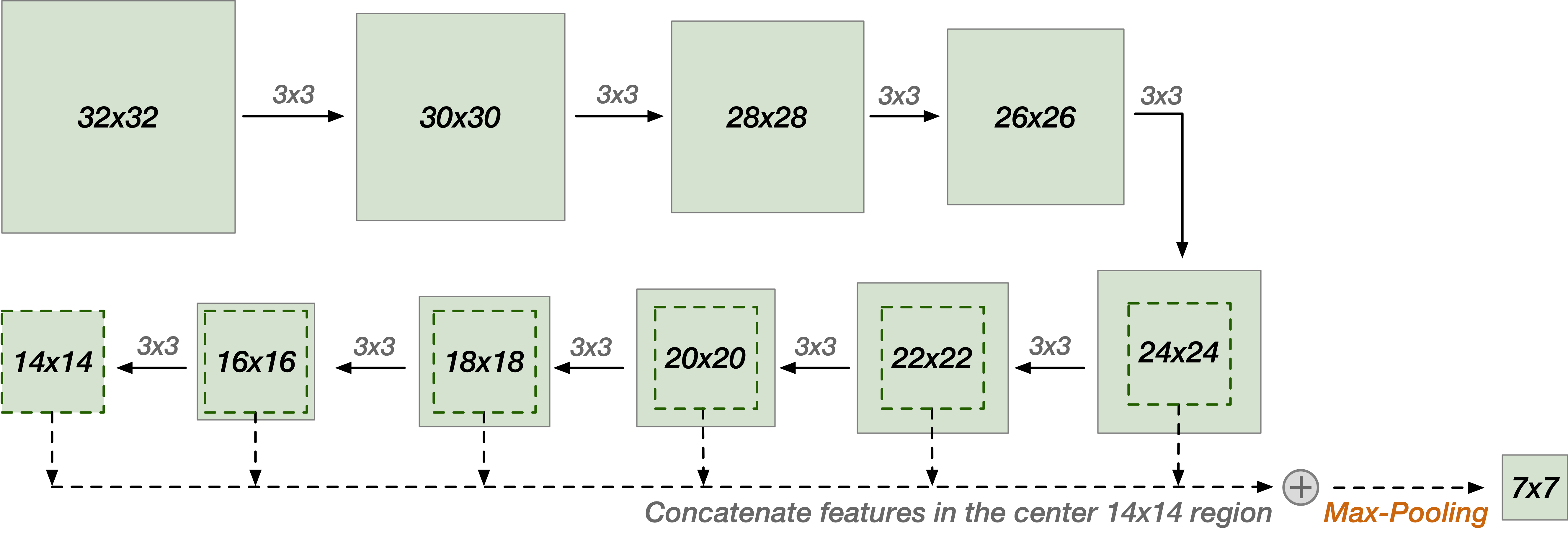
  Figure 1: Illustration of the context vector extraction procedure, where only the spatial dimension is shown.

• Attention window selection:
  After obtaining the context vector for each pixel, pixel-level classification is conducted to yield soft-decision scores, which will be used to estimate the discriminant power of each pixel. To reduce the complexity, we do a (2x2)-to-(1x1) max-pooling to generate 7x7 sparser pixels in an image. Image labels are used as pixel labels in the training phase. In the inference phase, the predicted soft decision is in form of a tensor of size 7x7x10, where 10 is the class number in CIFAR-10. To get aligned with the spatial resolution in the deepest hop unit, bilinear interpolation is applied to the soft decision channel-wise in order to increase its spatial resolution by two. Then, we can compute the confidence level for each pixel in the 14x14 region. The confidence level is defined as the inverse probability of most probable class based on the soft decision vector at the pixel. The higher the confidence level, the pixel is more discriminant for the top class in the soft decision. The most discriminant pixel from the 14x14 region is selected as the center of the attention window and its neighborhood of size WxW is set as the preliminary attention window, where W is an odd number.

The hyper-parameter, $W$, is set to 19 for the CIFAR-10 dataset in this work, which is equal to the size of the receptive field in the deepest hop. Note also that the spatial resolution of CIFAR-10 images is 32x32, which is already small and cropped for the object. On one hand, if the attention window size is larger than 19x19, it would be very close to the original input. On the other hand, if the attention window size is significantly smaller than 19x19, it would not be stable and/or reliable.

3.2 Step 2: Attention Map Refinement

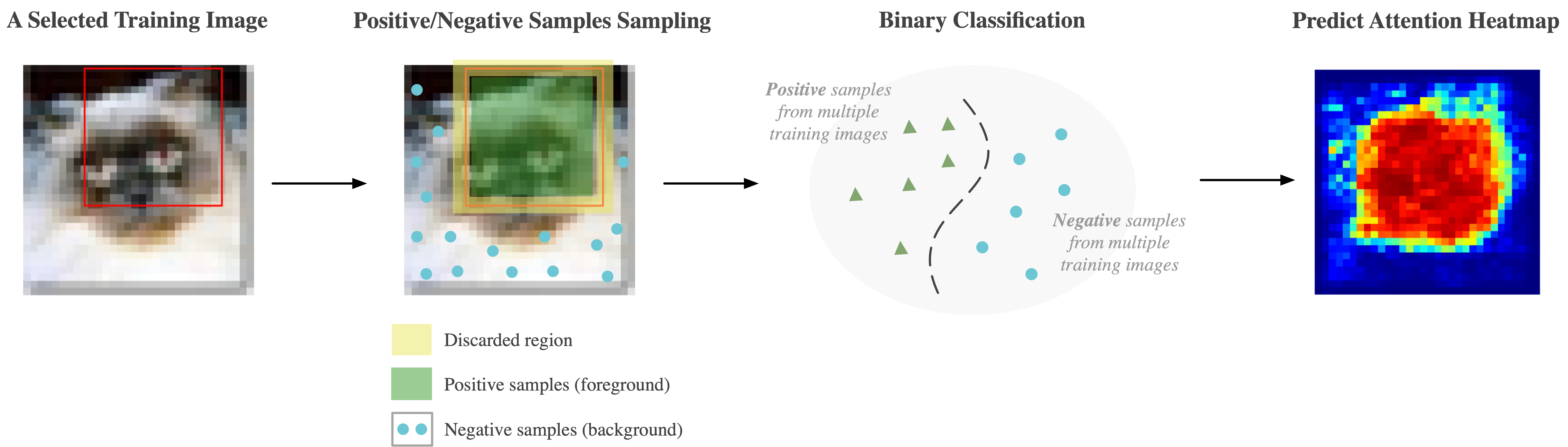
Figure 2: Illustration of the attention map refinement step.

Although the attention region of an input can be well localized in Step 1, the 19x19 squared window is not ideal for all images due to the variation of object sizes, shapes and orientations. We adopt a weakly supervised scheme to refine the attention map as illustrated in Fig. 2. It is formulated as a binary classification problem between the positive class (i.e., attention or foreground pixels) and the negative class (i.e., background pixels). The refined attention map is the area with a higher positive class probability.

Given a selected subset of training images, we sample from preliminary attention windows. Pixels inside the windows are labeled with the positive class. As to the negative class, since the pixel number outside the window is larger than that of inside the window, we apply random sampling to the outside region to balance the positive and negative sample numbers. Furthermore, we discard pixels along the boundaries of the attention windows within a certain distance threshold (say, 3 pixels) since their features are similar with each other. These pixels are treated as noisy samples and are not included in model training.

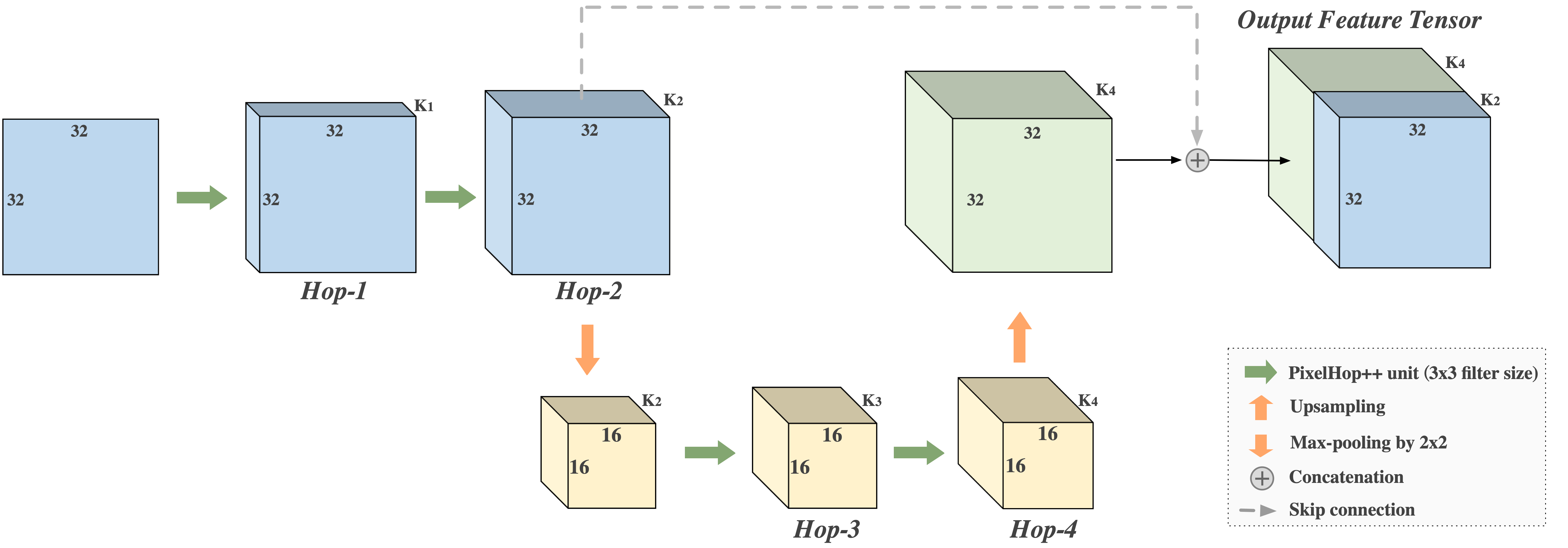
Figure 3: Illustration of feature extraction in the attention map refinement step.

In implementation, we use four cascaded PixelHop++ units to extract features for the binary classification as shown in Fig. 3. Padding is used before each hop unit to keep the resolution unchanged. To combine features from multiple scales for the same spatial location, channel-wise upsampling by a factor of 2 is applied to the Hop-4 feature map. Hop-4 features have a larger receptive field. They are concatenated with Hop-2 features that have a smaller receptive field through skip connection. The output feature tensor has a good balance between global and local representations.

3.3 Step 3: Attention Region Finalization

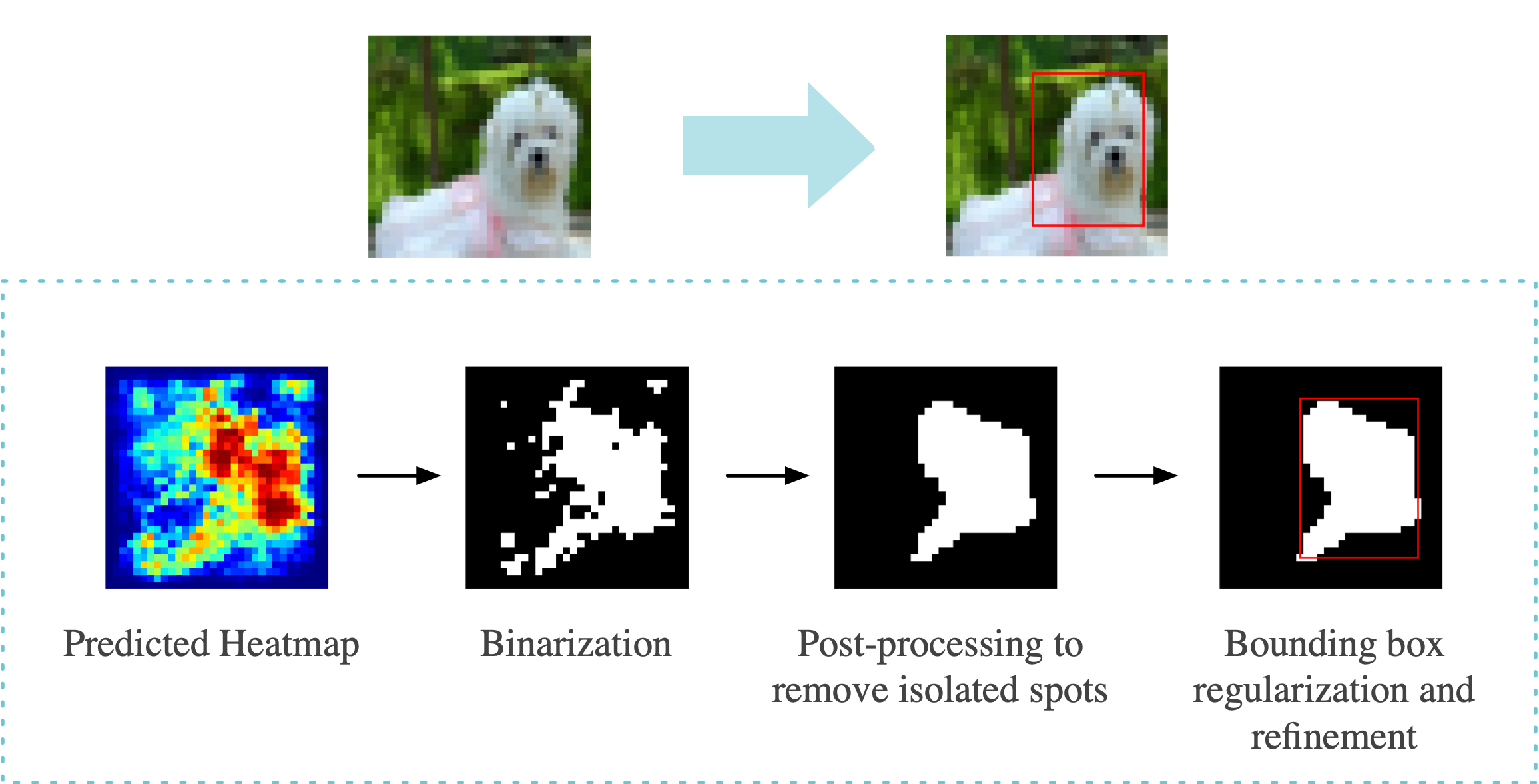
Figure 4: Illustration of the attention region finalization step.

Given the refined attention map from Step 2, we attempt to obtain a rectangular attention region that is adaptive to various object sizes and shapes in Step 3. As illustrated in Fig. 4, its processing consists of the following three substeps.

• Attention map binarization and cleaning:
  The soft decision scores in the attention map represent the probability of each pixel to be a foreground pixel. We set a uniform threshold $T_{att}$ to binarize the decision values. Empirically, we use $T_{att}=0.5$. To remove the isolated spots, we apply a median filter with radius 3 to each pixel.

• Bounding box regularization:
  The attention region is a rectangular one. We apply the maximum-occupancy-rate pooling strategy to derive the tightest bounding box that includes foreground pixels after the above substep. The estimated bounding box is regularized with its center location and its height $H$ and width $W$. To avoid extremely small bounding boxes, if $\max(H,W)$ is smaller than a threshold, the bounding box is enlarged to $\max(H,W)=16$ while keeping the aspect ratio unchanged.

• Final attention region extraction and resizing:
  Based on the regularized bounding box, the corresponding region is cropped out from the whole image. It is resized using the Lanczos interpolation to the same resolution as the original input image, for example, 32x32 for the CIFAR-10 dataset.

3.4 SAL-Assisted E-PixelHop

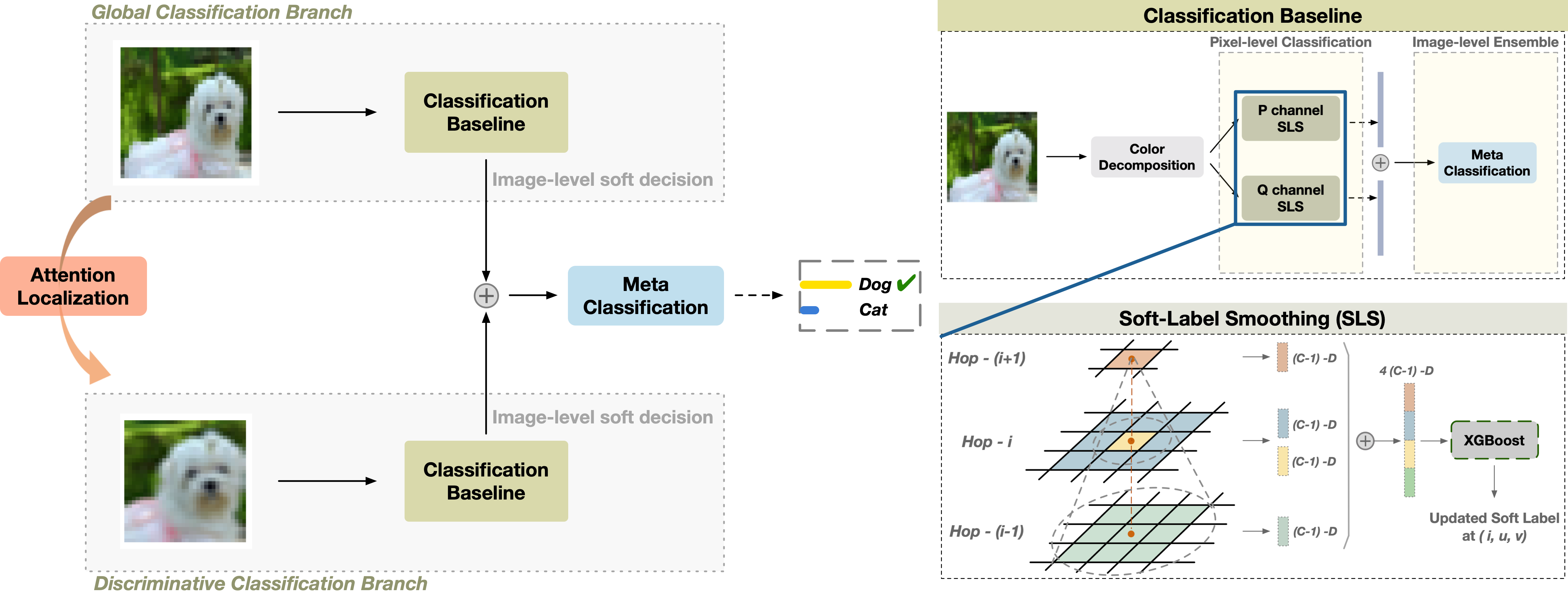
Figure 5: An overview of SAL-assisted E-PixelHop.

As an application of SAL, we propose an object classification pipeline with attention localization, named SAL-assisted E-PixelHop. It contains a two-stage decision pipeline: 1) multi-class classification and 2) binary-class classfication among the top two contenders.

In Stage 1, we adopt E-PixelHop [1] as the baseline (see Fig. 5 right subfigure), which is an SSL-based object classification solution. The color representation is first converted from the RGB space to the PQR space [1]. Soft-label smoothing (SLS) [1] is performed using cross-hop label update for reliable local decisions. Pixel classification is conducted based on smoothed soft labels. Then, pixel-wise decisions are flattened and ensembled through a meta classifier for image label prediction. However, there is one minor difference in this work. That is, the classification model is trained for a second round on hard samples to further boost the performance of E-PixelHop.

Fig. 5 illustrates the pipeline of Stage 2. It is only applied to the top 2 contenders after Stage 1, which is called the confusing set. For 10 object classes, there are at most 45 confusion sets. Stage 2 has two branches: the global classification and the attention classification. The former takes the whole image as its input while the latter takes the cropped-out and resized attention region obtained from SAL as input. Furthermore, classification results of both branches are ensembled through a logistic regression, which offers the highest classification accuracy.

4 Experiments

We visualize results obtained by SAL and conduct the performance of the attention-based object classification task in this section. Our experiments are carried out on the CIFAR-10 [27] dataset, which contains 10 classes of tiny color images of spatial resolution $32\times 32$ with 50,000 training and 10,000 test images.

Visualization of SAL Results. We show the preliminary attention extraction results (i.e., after Step 1 of SAL) of 10 test images in Fig. 6, where the red bounding boxes indicate a squared attention window of size $19\times 19$. We see that it can localize salient regions of an object quite well even without Steps 2 and 3. However, the bounding box of a fixed size may not fit the object tightly for some images (e.g., the rightmost image in the second row.) Figs. 7 and 8 show examples after attention refinement and rectangular attention region finalization for non-animal and animal objects, respectively. Each row has four subfigures. From left to right, they are the input image, the attention map (i.e., after Step 2 of SAL), the finalized attention region, and the cropped-out and resized attention image. It is shown qualitatively in these examples that SAL can capture salient regions of low resolution images well. It is robust to both large and small objects of various rectangular shapes.

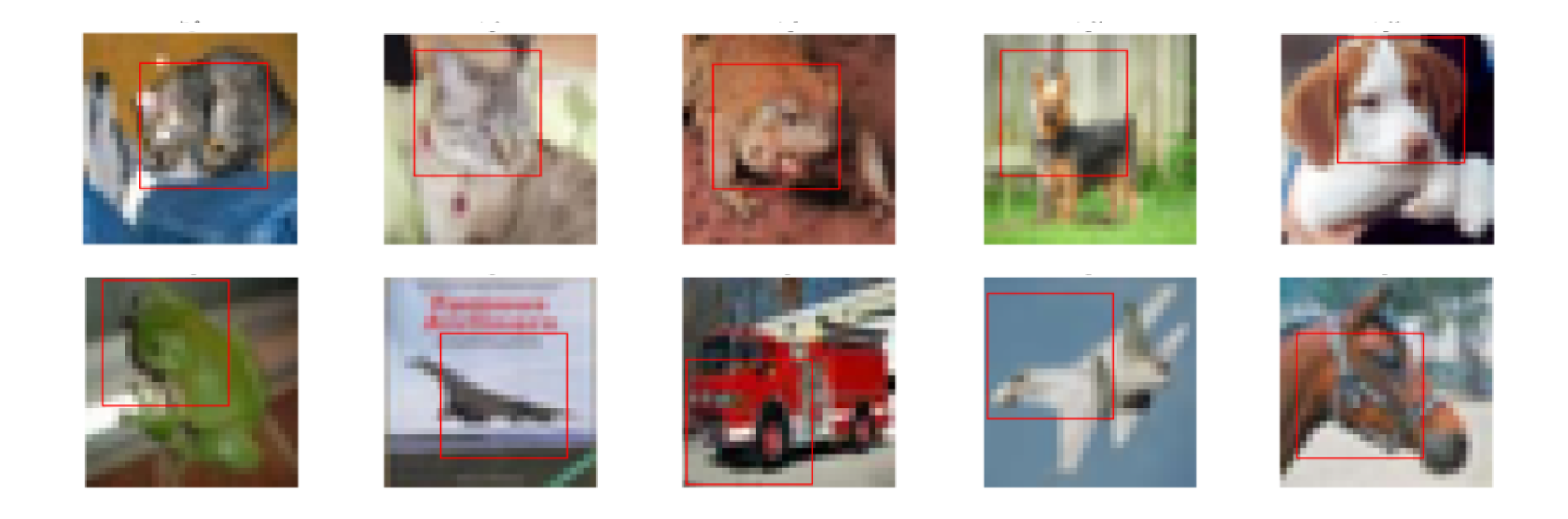
Figure 6: Results of preliminary attention windows for test images as indicated by red bounding boxes.

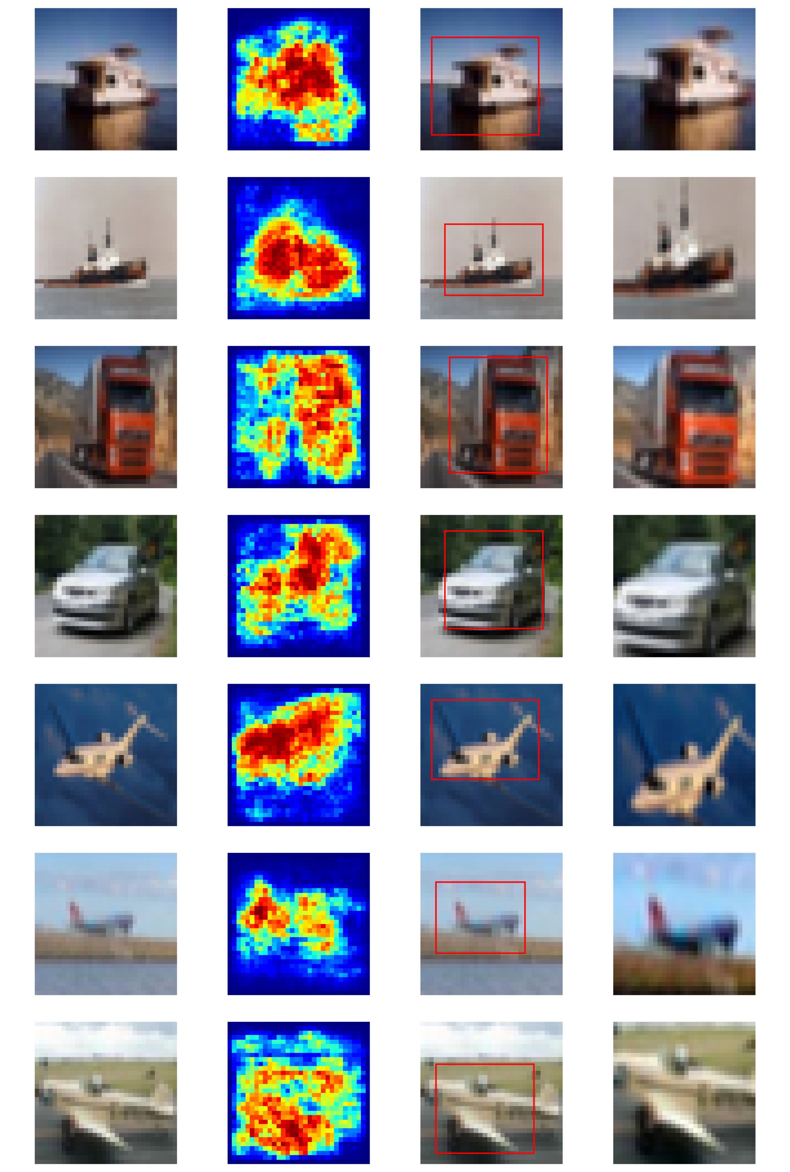
Figure 7: Visualization of SAL results for non-animal images (from left to right): the input image, the attention map (after Step 2 of SAL), the finalized attention region, and the cropped-out and rescaled image.

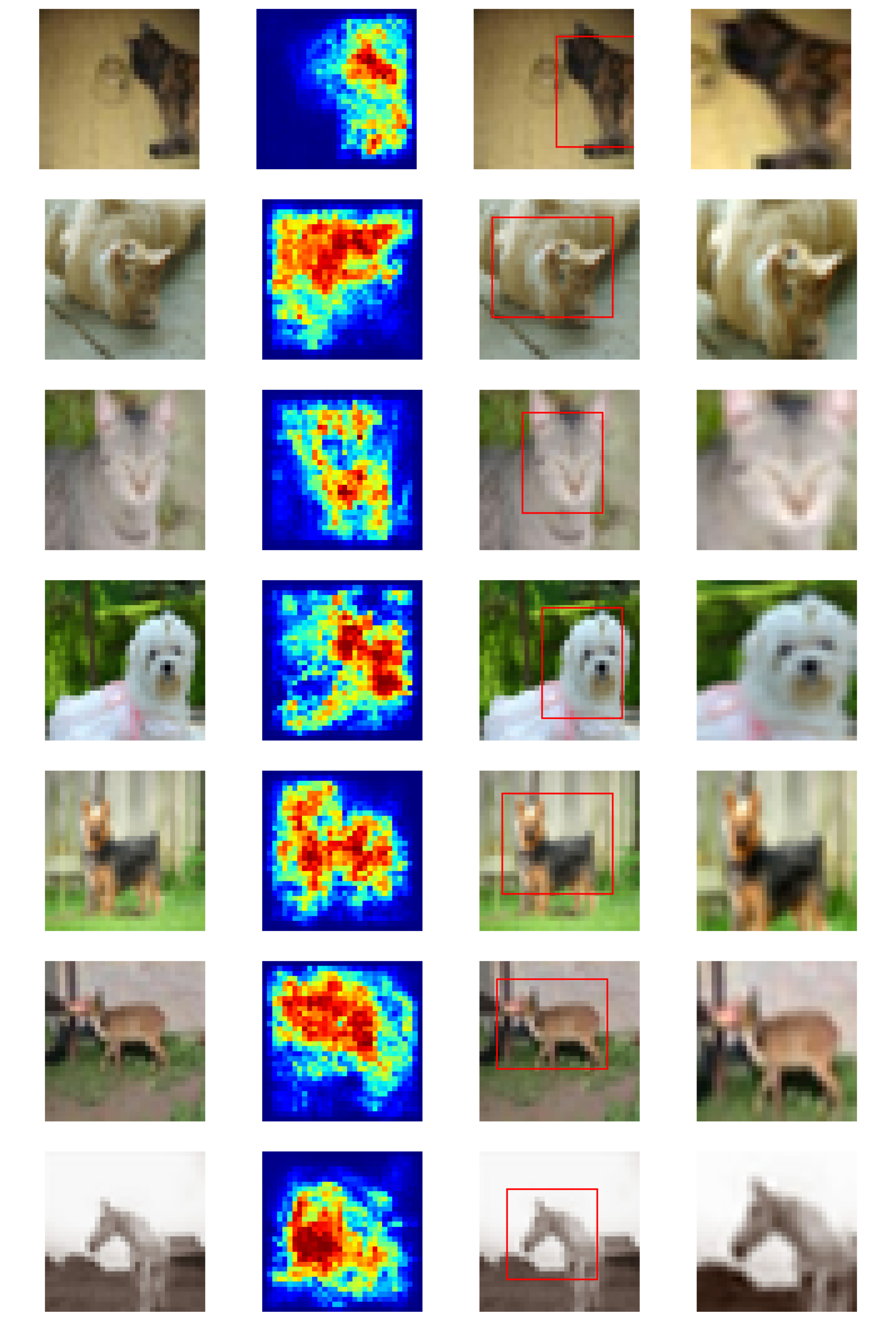
Figure 8: Visualization of SAL results for animal images (from left to right): the input image, the attention map (after Step 2 of SAL), the finalized attention region, and the cropped-out and rescaled image.

Two-Class Object Classification. Among the $10$ object classes in CIFAR-10, the four most challenging pairs are Cat/Dog, Airplane/Ship, Automobile/Truck, and Deer/Horse. There are 10K training images and 2K test images in each pair. The challenges come from high similarity in object shape (e.g. the pose and the natural body outline between cats and dogs, or deers and horses) as well as color tone of foreground or background (e.g. the blue sky for airplanes and blue ocean for ships). We focus on these four pairs to evaluate the performance of SAL-assisted binary object classification.

We show the performance of two-class object classification in Table 1. It gives the test accuracy for each pair under three scenarios: (1) classification based on original images only; (2) classification based on attention regions only; (3) ensemble results of (1) and (2). On one hand, we see that results with attention regions alone are not as competitive as those of the whole images in three out of four cases. This is because that CIFAR-10 images are tiny low-resolution images, where the full images already focus on objects. The contribution of attention may not be that visible. On the other hand, one can see that the ensemble results outperform the best of the first two. Thus, it means that SAL provides meaningful auxiliary information for higher classification accuracy.

Furthermore, we compare another eleven pairs among fifteen most confusing pairs in Fig. 9. We see from the figure that the attention region obtained by SAL yields better classification results than those based on the full images in ten (out of eleven) confusing pairs. This provides another evidence of the power of SAL. Again, the ensemble results perform the best.

Table 1: Comparison of image-level test accuracy (%) of the binary object classification with and without attention localization

	Full Frame	Cropped Attention	Ensemble
Cat vs Dog	79.10	77.90	80.05
Airplane vs Ship	93.75	92.20	94.10
Automobile vs Truck	92.95	93.45	93.90
Deer vs Horse	90.95	90.30	92.30

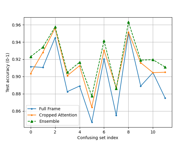
Figure 9: Comparison of classification accuracy of test images for another 11 confusion pairs among the top 15 confusing ones, where the 4 pairs reported in Table 1 are excluded.

Ten-Class Object Classification. For a 10-class classification problem, we consider a two-stage decision pipeline. For the first-stage classification, we conduct a baseline 10-class object classification task and assign each test a soft-decision vector of 10 dimensions, where each dimension indicates the probabilities of belonging to one class. Images with the same top-2 candidate classes in the baseline decision form one confusion set. There are at most 45 confusion sets for one-versus-one competition. The image number in each confusion set varies. For the second-stage classification, we focus on confusion sets that have a large number of images and conduct the two-class classification task. The class with a higher probability is chosen to be the final decision.

The ablation study of adopting various strategies is summarized in Table 2. Our study focuses on the stage-2, which includes the selected number of resolved confusion sets (25 or 45), the use of full images only, the use of attention regions only, the ensemble of the two. The final test accuracy for CIFAR-10 is given in the last column. When resolving all 45 confusion sets, the accuracy of stage-2 with ensembles can outperform that without SAL at all by 1.06%.

Table 2: Ablation study of 10-class classification accuracy with different decision strategies for CIFAR-10.

Stage-1	Stage-2				Test Accuracy
	# of Resolved	Full	Cropped	Ensemble
	Confusing Sets	Frame	Attention
✓					76.54
✓	25	✓			77.62
✓	25		✓		77.36
✓	25			✓	78.60
✓	45	✓			77.72
✓	45		✓		77.49
✓	45			✓	78.78

Finally, we compare the performance of modified LeNet-5  [24] and four SSL-based classification systems on CIFAR-10 in Table 3. The four SSL-based solutions include PixelHop [25], PixelHop⁺ [25], PixelHop++ [26], and E-PixelHop [1]. The two proposed SAL-assisted E-PixelHop methods outperform all other benchmarking methods.

Table 3: Comparison of testing accuracy (%) of LeNet-5, PixelHop, PixelHop⁺, PixelHop++, E-PixelHop and the proposed SAL-assisted E-PixelHop on CIFAR-10.

	Test Accuracy (%)
Lenet-5	68.72
PixelHop [25]	71.37
PixelHop+ [25]	72.66
PixelHop++ [26]	66.81
E-PixelHop [1]	76.18
Ours - 25 Resolved Sets	78.60
Ours - 45 Resolved Sets	78.78

5 Conclusion and Future Work

An SAL method to extract a distinctive object region was proposed in this work. It was shown by experiments that SAL can localize attention regions well for objects of various sizes and shapes in low resolution images. SAL was used to enhance the performance of an object classification baseline, E-PixelHop. The SAL-assisted E-PixelHop outperforms all existing SSL-based classification systems for the CIFAR-10 dataset. In the future, we plan to apply SAL to object images of higher resolution such as ImageNet.

References

- [1] Y. Yang, V. Magoulianitis, and C.-C. J. Kuo, “E-pixelhop: An enhanced pixelhop method for object classification,” arXiv preprint arXiv:2107.02966, 2021.
- [2] M. D. Zeiler and R. Fergus, “Visualizing and understanding convolutional networks,” in European conference on computer vision, pp. 818–833, Springer, 2014.
- [3] B. Zhou, Y. Sun, D. Bau, and A. Torralba, “Interpretable basis decomposition for visual explanation,” in Proceedings of the European Conference on Computer Vision (ECCV), pp. 119–134, 2018.
- [4] Q. Zhang, Y. N. Wu, and S.-C. Zhu, “Interpretable convolutional neural networks,” in Proceedings of the IEEE Conference on Computer Vision and Pattern Recognition, pp. 8827–8836, 2018.
- [5] B. Zhou, A. Khosla, A. Lapedriza, A. Oliva, and A. Torralba, “Learning deep features for discriminative localization,” in Proceedings of the IEEE conference on computer vision and pattern recognition, pp. 2921–2929, 2016.
- [6] P. H. Seo, Z. Lin, S. Cohen, X. Shen, and B. Han, “Progressive attention networks for visual attribute prediction,” arXiv preprint arXiv:1606.02393, 2016.
- [7] S. Jetley, N. A. Lord, N. Lee, and P. H. Torr, “Learn to pay attention,” arXiv preprint arXiv:1804.02391, 2018.
- [8] D. Lin, X. Shen, C. Lu, and J. Jia, “Deep lac: Deep localization, alignment and classification for fine-grained recognition,” in Proceedings of the IEEE conference on computer vision and pattern recognition, pp. 1666–1674, 2015.
- [9] L. Wang, Z. Wu, S. Karanam, K.-C. Peng, R. V. Singh, B. Liu, and D. N. Metaxas, “Sharpen focus: Learning with attention separability and consistency,” in Proceedings of the IEEE/CVF International Conference on Computer Vision, pp. 512–521, 2019.
- [10] N. Zhang, J. Donahue, R. Girshick, and T. Darrell, “Part-based r-cnns for fine-grained category detection,” in European conference on computer vision, pp. 834–849, Springer, 2014.
- [11] S. Huang, Z. Xu, D. Tao, and Y. Zhang, “Part-stacked cnn for fine-grained visual categorization,” in Proceedings of the IEEE conference on computer vision and pattern recognition, pp. 1173–1182, 2016.
- [12] S. Branson, C. Wah, F. Schroff, B. Babenko, P. Welinder, P. Perona, and S. Belongie, “Visual recognition with humans in the loop,” in European Conference on Computer Vision, pp. 438–451, Springer, 2010.
- [13] J. Deng, J. Krause, and L. Fei-Fei, “Fine-grained crowdsourcing for fine-grained recognition,” in Proceedings of the IEEE conference on computer vision and pattern recognition, pp. 580–587, 2013.
- [14] K. Duan, D. Parikh, D. Crandall, and K. Grauman, “Discovering localized attributes for fine-grained recognition,” in 2012 IEEE conference on computer vision and pattern recognition, pp. 3474–3481, IEEE, 2012.
- [15] C. Wang, W. Ren, K. Huang, and T. Tan, “Weakly supervised object localization with latent category learning,” in European Conference on Computer Vision, pp. 431–445, Springer, 2014.
- [16] D. J. Crandall and D. P. Huttenlocher, “Weakly supervised learning of part-based spatial models for visual object recognition,” in European conference on computer vision, pp. 16–29, Springer, 2006.
- [17] M. Oquab, L. Bottou, I. Laptev, and J. Sivic, “Is object localization for free?-weakly-supervised learning with convolutional neural networks,” in Proceedings of the IEEE conference on computer vision and pattern recognition, pp. 685–694, 2015.
- [18] R. G. Cinbis, J. Verbeek, and C. Schmid, “Weakly supervised object localization with multi-fold multiple instance learning,” IEEE transactions on pattern analysis and machine intelligence, vol. 39, no. 1, pp. 189–203, 2016.
- [19] L. Bazzani, A. Bergamo, D. Anguelov, and L. Torresani, “Self-taught object localization with deep networks,” in 2016 IEEE winter conference on applications of computer vision (WACV), pp. 1–9, IEEE, 2016.
- [20] X. Zhang, H. Xiong, W. Zhou, W. Lin, and Q. Tian, “Picking deep filter responses for fine-grained image recognition,” in Proceedings of the IEEE conference on computer vision and pattern recognition, pp. 1134–1142, 2016.
- [21] C.-C. J. Kuo, “Understanding convolutional neural networks with a mathematical model,” Journal of Visual Communication and Image Representation, vol. 41, pp. 406–413, 2016.
- [22] C.-C. J. Kuo, “The cnn as a guided multilayer recos transform [lecture notes],” IEEE signal processing magazine, vol. 34, no. 3, pp. 81–89, 2017.
- [23] C.-C. J. Kuo and Y. Chen, “On data-driven saak transform,” Journal of Visual Communication and Image Representation, vol. 50, pp. 237–246, 2018.
- [24] C.-C. J. Kuo, M. Zhang, S. Li, J. Duan, and Y. Chen, “Interpretable convolutional neural networks via feedforward design,” Journal of Visual Communication and Image Representation, 2019.
- [25] Y. Chen and C.-C. J. Kuo, “Pixelhop: A successive subspace learning (ssl) method for object recognition,” Journal of Visual Communication and Image Representation, vol. 70, p. 102749, 2020.
- [26] Y. Chen, M. Rouhsedaghat, S. You, R. Rao, and C.-C. J. Kuo, “Pixelhop++: A small successive-subspace-learning-based (ssl-based) model for image classification,” in 2020 IEEE International Conference on Image Processing (ICIP), pp. 3294–3298, IEEE, 2020.
- [27] A. Krizhevsky and G. Hinton, “Learning multiple layers of features from tiny images,” tech. rep., University of Toronto, Toronto, Ontario, 2009.