VQ-T: RNN Transducers using Vector-Quantized Prediction Network States

Abstract

Beam search, which is the dominant ASR decoding algorithm for end-to-end models, generates tree-structured hypotheses. However, recent studies have shown that decoding with hypothesis merging can achieve a more efficient search with comparable or better performance. But, the full context in recurrent networks is not compatible with hypothesis merging. We propose to use vector-quantized long short-term memory units (VQ-LSTM) in the prediction network of RNN transducers. By training the discrete representation jointly with the ASR network, hypotheses can be actively merged for lattice generation. Our experiments on the Switchboard corpus show that the proposed VQ RNN transducers improve ASR performance over transducers with regular prediction networks while also producing denser lattices with a very low oracle word error rate (WER) for the same beam size. Additional language model rescoring experiments also demonstrate the effectiveness of the proposed lattice generation scheme.

Index Terms: Lattice Generation; RNN Transducer; Vector-quantized LSTM

1 Introduction

End-to-end automatic speech recognition (ASR) has been a hot research direction. An end-to-end system directly maps acoustic features to linguistic units, reducing the workload of combining different knowledge sources. At the same time, it has shown equivalent or better performance over conventional hidden Markov model (HMM) based approaches [1, 2, 3]. According to recent literature, we have observed two mainstream modeling directions for end-to-end ASR: attention-based encoder-decoder (AED) [4, 5, 6], and RNN transducer (RNN-T) [7, 8, 9].

Beam search has been the main decoding strategy for both HMM-based approaches and end-to-end systems. Using a limited beam size $\mathcal{H}$, the search generates an $N$-best list with a computational cost of $\mathcal{O}(\mathcal{H})$. However, $N$-best lists are insufficient for some downstream applications or post-processing stages, such as (1) language model rescoring [10, 11, 12]; (2) downstream processing of ASR output (e.g., translation[13] and keyword spotting [14, 15]); (3) confusion network generation [16, 17]; and (4) sequence discriminative training [18, 19, 20].

Hypothesis merging (or path recombination) is the main difference between regular beam search and lattice-based search. For conventional methods, Rybach et al. divided merging procedures into two categories [12]: the phone-pair approach [10, 21] and the $N$-best history approach [22, 23, 24]. However, neither are suitable for end-to-end models because they require additional n-gram language models and HMM-based acoustic models to generate lattices. In order to generate lattices for end-to-end ASR models, recent works proposed approaches that restrict the hypothesis merging context [25, 26] with convolutional and recurrent decoders. Zapotoczny et al. [25] replaced the recurrent decoder with a temporal convolutional network (TCN) in AED networks. Since there is a fixed-length context, this method can merge hypotheses as efficiently as with an n-gram language model. Their experiments on the WSJ dataset indicate that character-based lattice decoding can consistently outperform beam decoding in terms of WER for a similar beam size. Prabhavalkar et al. [26] further investigated hypothesis merging for recurrent neural network transducer (RNN-T) with a full-context prediction network. They approximately merge hypotheses with the same last few byte pair encoding (BPE) labels, showing improvements in both 1-best and oracle WER.

This work proposes the use of vector-quantized long short-term memory units (VQ-LSTM) to generate lattices for RNN-Ts. The VQ layers are added to the LSTM cells and are jointly optimized with the transducer objective. We show that, with VQ-LSTM, we can actively merge hypotheses for lattice generation while conditioning on the full context. We investigate both systems in [25, 26], and provide a comparison for different types of encoders (LSTM and conformer) and linguistic units (characters and BPE units). Experiments on the Switchboard 300 hours corpus show that our method improves ASR performance on multiple test sets despite using compressed context information. The method also results in denser lattices with a significantly lower oracle WER. The generated lattices from VQ-based systems show improvements for language model rescoring as a downstream task.

2 RNN Transducer Formulation

In RNN-T, the objective function to be minimized is the negative log-likelihood (NLL) loss, defined as $-\log p(\bm{{y}}|\bm{{x}})$ [7, 27]. $\bm{{x}}=(x_{1},...,x_{T})$ is an input speech feature sequence with length $T$, and $\bm{{y}}=(y_{0},y_{1},...,y_{U})$ is an output label sequence with length $U+1$, where $y_{u}\in\mathcal{Y}$ with label vocabulary $\mathcal{Y}$ and $y_{0}$ is the start token of a label sentence. Symbol prediction probability $p(\bm{{y}}|\bm{{x}})$ can be elaborated into the summation over all possible alignments $\bm{{a}}$:

$$p(\bm{{y}}|\bm{{x}})=\sum_{\bm{{a}}\in\mathcal{B}^{-1}(\bm{{y}})}p(\bm{{a}}|\bm{{x}})$$ (1)

where $\bm{{a}}\in\mathcal{Y}\cup\{\phi\}$ is a sequence of symbols augmented by blank symbols $\phi$, and function $\mathcal{B}$ maps alignment $\bm{{a}}$ to the output sequence $\bm{{y}}$. The speech features $\bm{{x}}$ are encoded into hidden states $\bm{{m}}=(m_{1},m_{2},...,m_{T})$ by an encoder network. The partial output sequence $\bm{{y}}_{u}=(y_{0},y_{1},...,y_{u-1})$ is encoded into hidden states $\bm{{g}}_{u}=(g_{1},g_{2},...,g_{u})$ by a prediction network.

$p(\bm{{a}}|\bm{{x}})$ is given by a joint network based on the following factorization:

$$\begin{split}p(\bm{{a}}|\bm{{x}})=p(\bm{{a}}|\bm{{m}})\triangleq\prod_{i=1}^{T+U}p(a_{i}|m_{t_{i}},\mathcal{B}(a_{1},...,a_{i-1}))=\\ =\prod_{i=1}^{T+U}p(a_{i}|m_{t_{i}},y_{0},...,y_{u_{i-1}})=\prod_{i=1}^{T+U}p(a_{i}|m_{t_{i}},g_{u_{i}}),\end{split}$$ (2)

where $t_{i}$ and $u_{i}$ are corresponding $t$ and $u$ at the alignment step $i$. Based on the factorization, the NLL loss can be efficiently computed with the forward-backward algorithm, which has computational complexity bounded by $\mathcal{O}(TU)$.

3 VQ-LSTM and Lattice Generation

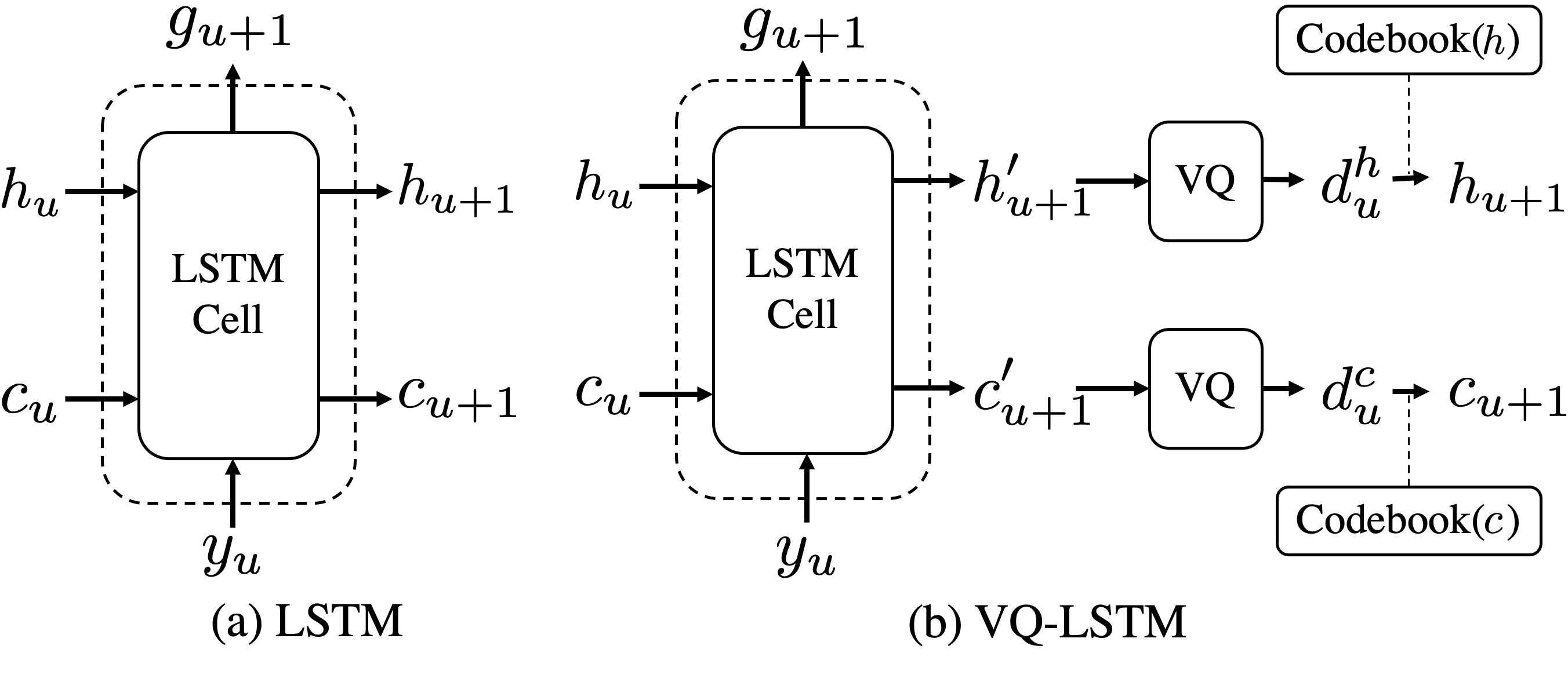
Figure 1: Structure comparison between LSTM and VQ-LSTM.

3.1 Very-limited-context (VLC) Model

As noted in Section 1, lattice generation in end-to-end ASR models relies on hypothesis merging. Compared to the RNN-T with full-context LSTM layers, several recent studies have found that the prediction network can achieve comparable performances with limited context or simple structures [26, 25, 28, 29]. Zapotoczny et al. [25] proposed to apply TCN for lattice generation in the attention-based encoder-decoder (AED) architecture so as to limit the context received in the decoder network. Following this direction, we employ simple convolutional layers in RNN-T prediction networks. We find a left context of only two tokens could already reach reasonable ASR performance, so we introduce this model as a reference model for our following discussion, namely as a very-limited-context (VLC) model.

3.2 VQ-LSTM

Hypothesis merging for lattice generation is straightforward in HMM-based hybrid systems thanks to the limited context in n-gram language models. However, the hidden state of LSTM prediction network for further expansion is a tuple of continuous vectors $h_{u}$ and $c_{u}$ at iteration $u$. A compromise is to train the LSTM-based prediction network only on a limited context, which has been shown to degrade performance [26]. As an alternative in this work, we apply vector quantization to the LSTM hidden and cell states.

Vector quantization (VQ) has been successfully applied in several areas, especially representation learning [30, 31, 32, 33], but more recently as a useful inductive bias [34] to enhance generalization. In most cases, the VQ process acts as a feature extractor, encoding intermediate hidden states from the network into a more compact discrete representation. Previous literature explored distilling the probabilistic model into a weighted finite state transducer (wFST) so as to perform rescoring for ASR and other natural language processing tasks [35, 36]. However, the performance of these methods is likely to be bounded by the performance of the original probabilistic model, given that the distillation was not optimized with the same objective as the probabilistic model.

In this work, we propose to apply a trainable VQ layer to the LSTM states to enable lattice generation without performance degradation for 1-best decoding. As illustrated in Fig. 1(b), we denote $h_{u},c_{u},g_{u}\in\mathbb{R}^{D}$, where $D$ is the dimension of corresponding vectors. Then, an iteration of original LSTM is defined as:

$$g_{u+1},(h_{u+1},c_{u+1})=\mathrm{LSTM}(y_{u},h_{u},c_{u}).$$ (3)

As shown in Fig. 1(b), to apply vector quantization to LSTM, we add two vector quantizers, resulting in a recurrent network with discrete hidden and cell states $d_{u}^{h}\in\mathbb{N},d_{u}^{c}\in\mathbb{N}$. With the quantizers, an iteration $u$ of VQ-LSTM is defined as:

$$g_{u+1},(h^{\prime}_{u+1},c^{\prime}_{u+1}) =\mathrm{LSTM}(y_{u},h_{u},c_{u}),$$ (4)

$$(d^{h}_{u},d^{c}_{u}) =\mathrm{VQ}(h^{\prime}_{u+1},c^{\prime}_{u+1})$$ (5)

$$(h_{u+1},c_{u+1}) =\mathrm{Codebook}(d^{h}_{u},d^{c}_{u}).,$$ (6)

The detailed implementation of $\mathrm{VQ}(\cdot)$ in Eq. (5) follows VQ-wav2vec [30]: we first employ a few fully-connected layers to project the states $h^{\prime}_{u+1},c^{\prime}_{u+1}$ into logits. Next, we apply GumbelSoftmax to convert the input vector into probability and use argmax to select the highest probability index as $d^{h}_{u},d^{c}_{u}$ in the related codebook. The corresponding vector obtained by $\mathrm{Codebook}(\cdot)$ in Eq. (6) is then passed to the joint network. The discrete representations $d^{h}_{u},d^{c}_{u}$ are used for the hypothesis merging step in lattice generation.

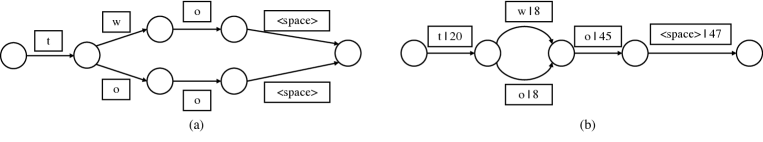
Figure 2: Lattice examples: (a) Very-limited-context (VLC) model from Sec 3.1. (b) VQ-based model from Sec 3.2 (numbers represent codebook indices). As shown in (b), VQ-based model can produce the same discrete code (i.e., $d^{h}_{u},d^{c}_{u}$), even when contexts are different.

3.3 Lattice Generation Algorithm

The VQ-based lattice generation is based on alignment length synchronous decoding (ALSD) with hypothesis merging [37]. Its pseudo code is shown in Algorithm 1.

The lattice $\mathcal{L}$ is initialized as an empty finite state acceptor (FSA). A hypothesis is defined by the tuple $(n,\bm{{y}}_{u},(h_{u},c_{u}),\delta_{t,u}(\bm{{y}}_{u}))$, consisting of its last node $n$ in the lattice, partial output sequence $\bm{{y}}_{u}$, prediction network states $(h_{u},c_{u})$, and hypothesis score $\delta_{t,u}(\bm{{y}}_{u})$. The score $\delta_{t,u}(\bm{{y}}_{u})$ stands for the posterior probability of sequence $\bm{{y}}_{u}$ at time $t$ and position $u$. As in [37], we define two hypothesis sets $A$ and $B$ to store beams of hypotheses for alignment steps $i$ and $i-1$, respectively. Hypothesis set $F$ is also introduced to store final hypotheses. The set $B$ starts with the initial hypothesis $(n_{\text{start}},\phi,(h_{0},c_{0}),1)$, while $A$ and $F$ start from an empty set.

Algorithm 1 VQ-based Lattice Generation

1:Encoder states: $\bm{{m}}$; Beam size: $\mathcal{H}$; Max output sequence length: $U_{max}$;

2:Hypotheses sorted by likelihood: $hyps$; Lattice: $\mathcal{L}$;

3:$\mathcal{L},n_{\text{start}},n_{\text{end}}=$FSA()

4:$B=\{(n_{\text{start}},\phi,(h_{0},c_{0}),1)\}$; $F=\{\}$; $A=\{\}$

5:for $i=1...T+U_{max}$ do

6:     $A=$ExpandHypothesis$(B,\bm{{m}})$

7:     $A,F=$MergeVQState$(A,\mathcal{H})$

8:     $B=$Prune$(A)$

9:     $\mathcal{L},B=$UpdateLattice$(B,\mathcal{L})$

10:end for

11:return sorted($F$) and $\mathcal{L}$;

During the main loop, the alignment step $i$ is iterated from $1$ to $T+U_{max}$, where $U_{max}$ is an estimate of the maximum output sequence length. The merge actions are recorded in lattice $\mathcal{L}$. Four major functions in Algorithm 1 include:

(1) ExpandHypothesis (line 4): each hypothesis is expanded over the vocabulary size $|\mathcal{Y}|$. Compared to the algorithm in [37], for all potential hypotheses, we apply additional prediction network forward-passes (i.e., Eq. (4) and Eq. (5)) to extract discrete context representations $(d^{h}_{u},d^{c}_{u})$ discussed in Sec. 3.2.

(2) MergeVQState (line 5): hypothesis merging with the same state (i.e., state code $(d^{h}_{u},d^{c}_{u})$ for VQ-based system). During the merge, the posterior probability is summed over merging hypotheses, and the hypothesis with the maximum probability are selected (i.e., keep its corresponding $(d^{h}_{u},d^{c}_{u})$ for the merged hypothesis) for further expansion.

(3) Prune (line 6): pruning with respect to beam size.

(4) UpdateLattice (line 7): updating lattice. For merged hypotheses, the additional arcs have the same target node, while for others, the arcs link to different target nodes.

The VLC model has similar lattice generation procedures, but it does not record $(d^{h}_{u},d^{c}_{u})$ over step $u$, nor does it perform the additional forward-pass in “ExpandHypothesis”.

Examples of generated lattices are shown in Figure 2. VLC needs to have same limited context (i.e., context of “o” “space” for hypothesis merging. The VQ-based model does not have this requirement and have the possibility of generating the same discrete hidden state (i.e., “8” for “w” and “o” in Fig. 2) for hypotheses merging.

4 Experiments

Model	StateNum	Encoder	Outputs	Evaluation (WER)
				Hub5’00	Hub5’01	RT’03
Baseline	$\infty$	LSTM	Char	11.8	12.1	15.3
			BPE	12.1	12.3	15.2
		Conformer	Char	11.4	11.2	14.4
			BPE	11.3	10.7	14.9
VLC	$|\mathcal{Y}|^{2}$	LSTM	Char	11.7	12.2	15.1
			BPE	11.4	12.1	14.9
		Conformer	Char	11.5	11.4	14.6
			BPE	11.4	10.9	14.5
VQ-T	6404	LSTM	Char	11.7	11.7	14.8
			BPE	12.0	12.1	15.1
		Conformer	Char	11.3	10.9	14.2
			BPE	11.1	10.9	13.6

Table 1: Word error rate (WER) at beam size 16 for different models: StateNum is the total number of states in prediction network. $|\mathcal{Y}|$ for VLC is the vocabulary size, which is 45 for characters and 681 for BPE units.

Model	Lattice Density
Baseline	31.5
VLC	25.4
VQ-T	165.5

Table 2: Lattice density at beam size 8 for models with LSTM encoders over characters.

4.1 Experimental Settings

Datasets: Experiments are conducted on the Switchboard speech corpus, which has 300 hours of English telephone conversations between two speakers on a preassigned topic. We use the same data segmentation and transcript preparation as the Kaldi s5c recipe [38]. For the evaluation set, we use the Hub5’00, Hub5’01, and RT’03 test sets with Kaldi-style measurement of the WER.

Features and data augmentation: We keep the same feature extraction setup and augmentation strategies as in [9]. To be specific, features are derived from log-Mel filter-bank features and i-vectors. Speed perturbation and SpecAugment are also applied during the training. We evaluate our models for both character and byte-pair encoding (BPE). The BPE units are extracted using 100-step byte-pair encoding. The vocabulary sizes $|\mathcal{Y}|$ for character and BPE models are 45 and 681, respectively.

Model architectures: Three models are used in the experiments: Baseline, VLC, and VQ-T. The Baseline model is an RNN-T which uses an encoder based on a stack of 6 bidirectional LSTMs with 640 units per layer per direction initialized with a model trained with connectionist temporal classification loss [39]. The prediction network is a single-layer unidirectional LSTM with 768 units (i.e., $D=768$). The joint network takes the input from the encoder and prediction networks and projects them into 256-dimensional vectors. The projected vectors are multiplied together element-wise [9], passed through a $\tanh$ activation, and projected to the vocabulary $\mathcal{Y}$ and blank symbol $\phi$. The Baseline with conformer encoders has the same prediction network configuration as Baseline, but the encoder has 12 layers, a hidden dimension of 384, a convolutional kernel of size 31, and six 96-dimensional attention heads per layer.

The VLC model adopts the same encoder architecture as Baseline, but with a convolutional prediction network. The prediction network in VLC has two parallel 256-dimensional-convolutional layers, one with a $\tanh()$ nonlinearity and one bias-free skip connection. Both have a two-linguistic-unit left context. The output of the prediction network is the sum of the two convolutional layers.

We perform vector quantization via GumbelSoftmax as introduced in [40]. Three hyper-parameters are introduced for the VQ layers: $vq\_group$ is the number of groups in each VQ layer; $vq\_vars$ is the number of codebook vectors per group; $vq\_depth$ is the number of fully connected layers before converting the input vector into logits. These three hyper-parameters have the strongest influence in our experiments, so other hyper-parameters such as training temperature and GumbelSoftmax coefficients are set to default settings from VQ-wav2vec. VQ-T follows the same architecture as Baseline, but with additional VQ layers in LSTM-based prediction networks. The default setting for VQ layer is with $vq\_group$ of 2, $vq\_vars$ of 640, $vq\_depth$ of 1. With these defaults, the total number of additional parameters introduced by the VQ-layer is less than 1M, less than 5% of the total model parameters.

Training: All models are trained on 2 V100 GPUs with minibatches of 32 utterances per GPU, the AdamW optimizer, and the OneCycle scheduler. VQ models are trained for 30 epochs, while the other models are trained for 20. The peak learning rate is 0.0005.

Decoding: In [37], the decoding algorithms for RNN-Ts are categorized into two types: time synchronous decoding (TSD) and ALSD. Experiments in [37] indicate that ALSD has similar accuracy as TSD, but is much faster. Therefore, we choose ALSD as our base decoding strategy.

Lattice generation: Both VLC and VQ-T models generate lattices by merging hypotheses with the same discrete hidden states, in contrast to [26] where full context prediction networks are used but hypotheses are merged based on the same limited context from running hypotheses. For comparison, we also generate lattices with Baseline by fixing the same context as VLC for merging. Since the lattice generation for VQ-T needs to conduct one extra forward pass for each decoding step, we only conduct experiments on character-based lattices for efficiency.

Language model rescoring: To evaluate the lattice quality, we also conduct language model rescoring over lattices. We apply a three-layer 512 dimensional LSTM language model trained on 25M words of the Fisher and Switchboard transcripts. We prune the VQ-T lattices before rescoring with a relative margin for arcs that share the same source and target node.

Evaluation metric: Besides WER for ASR performance, we adopt two metrics for lattice evaluation: lattice density and oracle WER. Lattice density is the average number of lattice arcs per frame. Oracle WER has been used to evaluate lattice quality by finding the lowest word error hypothesis in the lattice.

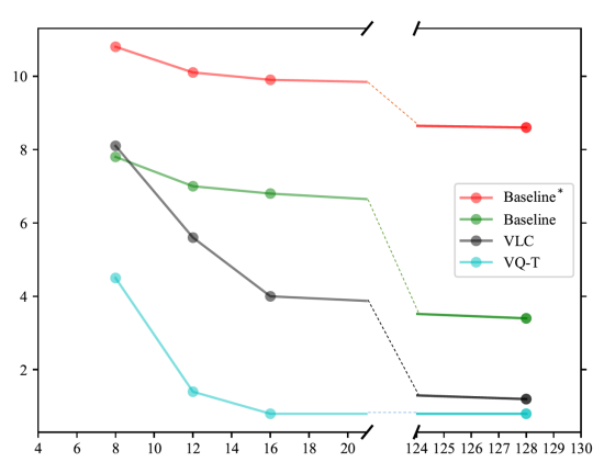
Figure 3: Oracle WER for models with different beam sizes: the models are with LSTM encoders over characters. Baseline^∗ is based on tree structure from beam search.

Model	LSTM	Conformer
Baseline	11.3(0.5)	11.0(0.4)
VLC	11.2(0.5)	10.9(0.6)
VQ-T	11.0(0.7)	10.8(0.5)

Table 3: Language model rescoring for character-based models on Hub5’00. Absolute improvements from rescoring are shown in parentheses.

4.2 Results and Discussion

The WER for different models is shown in Table 1. The VQ-T model with conformer encoders over BPE units reaches the overall best performance of 11.1 and 13.6 for Hub5’00 and RT’03. We also observe similar performances on Hub5’01 to the baseline with full context. Aligning with findings in [28, 29], VLC model performs comparably to the Baseline model. At the same time, the learnable VQ-T model performs slightly better in most cases.

Table 2 shows the lattice density for three sample models with LSTM encoders over characters. Compared to other models, our proposed VQ-T models have significantly denser lattices. The major reason is that VQ-T performs more active hypothesis merging for similar context. Fig.3 illustrates the oracle WER from lattices generated from the three models over different beam sizes. The results are similar to Table 2. Because of the denser lattices, the VQ-T oracle WERs converge considerably faster when increasing the beam size. We also observe much lower oracle WERs at convergence for VQ-T systems.

Table 3 shows the WER from lattice rescoring. While rescoring leads to better transcription accuracy in all cases, the best performance is obtained with the VQ-T models.

5 Conclusion and Future Work

In this work, we use vector-quantization of prediction network states to simplify lattice generation with RNN-Ts. The method efficiently compresses full context into discrete states, providing natural merge points for hypothesis merging in lattice generation. Our experiments on the Switchboard conversational corpus show that the proposed VQ-based transducer improves the performance of beam search 1-best decoding and generates dense, efficient lattices with a very low oracle WER for small beam sizes. We also verify the lattice quality using language model rescoring as a downstream task. One major challenge with the proposed method, however, is the increased decoding time, given that we introduce extra forward steps in the lattice generation algorithm. Since the forward pass needs to iterate over the entire vocabulary set, it is diffcult to extend the lattice generation to BPE units or words. Therefore, our future work will focus on improving decoding and VQ-based lattice generation efficiency with BPE units. Another direction is to use the lattices for more downstream tasks (e.g., translation, keyword spotting, and confusion network processing).

References

- [1] C.-C. Chiu, T. N. Sainath, Y. Wu, R. Prabhavalkar et al., “State-of-the-art speech recognition with sequence-to-sequence models,” in ICASSP, 2018, pp. 4774–4778.
- [2] N.-Q. Pham, T.-S. Nguyen, J. Niehues, M. Müller et al., “Very deep self-attention networks for end-to-end speech recognition,” Interspeech, pp. 66–70, 2019.
- [3] P. Guo, F. Boyer, X. Chang, T. Hayashi et al., “Recent developments on espnet toolkit boosted by conformer,” in ICASSP, 2021, pp. 5874–5878.
- [4] J. K. Chorowski, D. Bahdanau, D. Serdyuk, K. Cho et al., “Attention-based models for speech recognition,” in NIPS, 2015, pp. 577–585.
- [5] W. Chan, N. Jaitly, Q. Le, and O. Vinyals, “Listen, attend and spell: A neural network for large vocabulary conversational speech recognition,” in ICASSP, 2016, pp. 4960–4964.
- [6] S. Watanabe, T. Hori, S. Kim, J. R. Hershey et al., “Hybrid ctc/attention architecture for end-to-end speech recognition,” IEEE Journal of Selected Topics in Signal Processing, vol. 11, no. 8, pp. 1240–1253, 2017.
- [7] A. Graves, “Sequence transduction with recurrent neural networks,” arXiv preprint arXiv:1211.3711, 2012.
- [8] K. Rao, H. Sak, and R. Prabhavalkar, “Exploring architectures, data and units for streaming end-to-end speech recognition with RNN-transducer,” in ASRU, 2017, pp. 193–199.
- [9] G. Saon, Z. Tüske, D. Bolanos, and B. Kingsbury, “Advancing RNN transducer technology for speech recognition,” in ICASSP, 2021, pp. 5654–5658.
- [10] A. Ljolje, F. Pereira, and M. Riley, “Efficient general lattice generation and rescoring,” in EuroSpeech, 1999.
- [11] H. Sak, M. Saraclar, and T. Güngör, “On-the-fly lattice rescoring for real-time automatic speech recognition,” in Interspeech, 2010.
- [12] D. Rybach, M. Riley, and J. Schalkwyk, “On lattice generation for large vocabulary speech recognition,” in ASRU, 2017, pp. 228–235.
- [13] G. Kumar, M. Post, D. Povey, and S. Khudanpur, “Some insights from translating conversational telephone speech,” in ICASSP, 2014, pp. 3231–3235.
- [14] B. Kingsbury, J. Cui, X. Cui, M. J. Gales et al., “A high-performance cantonese keyword search system,” in ICASSP, 2013, pp. 8277–8281.
- [15] A. Rosenberg, K. Audhkhasi, A. Sethy, B. Ramabhadran et al., “End-to-end speech recognition and keyword search on low-resource languages,” in ICASSP, 2017, pp. 5280–5284.
- [16] L. Mangu, E. Brill, and A. Stolcke, “Finding consensus in speech recognition: word error minimization and other applications of confusion networks,” CSL, vol. 14, no. 4, pp. 373–400, 2000.
- [17] D. Hakkani-Tür, F. Béchet, G. Riccardi, and G. Tur, “Beyond asr 1-best: Using word confusion networks in spoken language understanding,” CSL, vol. 20, no. 4, pp. 495–514, 2006.
- [18] Y. Normandin, “Maximum mutual information estimation of hidden markov models,” in ASRU, 1996, pp. 57–81.
- [19] D. Povey and P. C. Woodland, “Minimum phone error and i-smoothing for improved discriminative training,” in ICASSP, 2002, pp. 100–105.
- [20] M. Gibson and T. Hain, “Hypothesis spaces for minimum bayes risk training in large vocabulary speech recognition.” in Interspeech, vol. 6, 2006, pp. 2406–2409.
- [21] M. Mohri, F. Pereira, and M. Riley, “Speech recognition with weighted finite-state transducers,” in Springer handbook of speech processing, 2008, pp. 559–584.
- [22] G. Saon, D. Povey, and G. Zweig, “Anatomy of an extremely fast lvcsr decoder,” in EuroSpeech, 2005.
- [23] S. F. Chen, B. Kingsbury, L. Mangu, D. Povey et al., “Advances in speech transcription at ibm under the darpa ears program,” TASLP, vol. 14, no. 5, pp. 1596–1608, 2006.
- [24] H. Soltau and G. Saon, “Dynamic network decoding revisited,” in ASRU, 2009, pp. 276–281.
- [25] M. Zapotoczny, P. Pietrzak, A. Łańcucki, and J. Chorowski, “Lattice Generation in Attention-Based Speech Recognition Models,” in Interspeech, 2019, pp. 2225–2229.
- [26] R. Prabhavalkar, Y. He, D. Rybach, S. Campbell et al., “Less is more: Improved RNN-t decoding using limited label context and path merging,” in ICASSP, 2021, pp. 5659–5663.
- [27] T. Bagby, K. Rao, and K. C. Sim, “Efficient implementation of recurrent neural network transducer in tensorflow,” in SLT, 2018, pp. 506–512.
- [28] E. Variani, D. Rybach, C. Allauzen et al., “Hybrid autoregressive transducer (hat),” in ICASSP. IEEE, 2020, pp. 6139–6143.
- [29] R. Botros, T. N. Sainath, R. David et al., “Tied & Reduced RNN-T Decoder,” in Proc. Interspeech 2021, 2021, pp. 4563–4567.
- [30] A. Baevski, S. Schneider, and M. Auli, “vq-wav2vec: Self-supervised learning of discrete speech representations,” arXiv preprint arXiv:1910.05453, 2019.
- [31] J. Chorowski, R. J. Weiss, S. Bengio, and A. van den Oord, “Unsupervised speech representation learning using wavenet autoencoders,” TASLP, vol. 27, no. 12, pp. 2041–2053, 2019.
- [32] E. Dunbar, J. Karadayi, M. Bernard, X.-N. Cao et al., “The zero resource speech challenge 2020: Discovering discrete subword and word units,” in Interspeech, 2020.
- [33] J. Robine, T. Uelwer, and S. Harmeling, “Smaller world models for reinforcement learning,” arXiv preprint arXiv:2010.05767, 2020.
- [34] D. Liu, A. Lamb, K. Kawaguchi et al., “Discrete-valued neural communication in structured architectures enhances generalization,” in Proc. NeurIPS, 2021.
- [35] G. Lecorvé and P. Motlicek, “Conversion of recurrent neural network language models to weighted finite state transducers for automatic speech recognition,” in Interspeech, 2012, pp. 1668–1671.
- [36] A. T. Suresh, B. Roark, M. Riley et al., “Approximating probabilistic models as weighted finite automata,” Computational Linguistics, vol. 47, no. 2, pp. 221–254, 2021.
- [37] G. Saon, Z. Tüske, and K. Audhkhasi, “Alignment-length synchronous decoding for RNN transducer,” in ICASSP, 2020, pp. 7804–7808.
- [38] D. Povey, A. Ghoshal, G. Boulianne, L. Burget et al., “The kaldi speech recognition toolkit,” in ASRU, 2011.
- [39] K. Audhkhasi, G. Saon, Z. Tüske, B. Kingsbury, and M. Picheny, “Forget a bit to learn better: Soft forgetting for ctc-based automatic speech recognition.” in Interspeech, 2019, pp. 2618–2622.
- [40] E. Jang, S. Gu, and B. Poole, “Categorical reparameterization with gumbel-softmax,” arXiv preprint arXiv:1611.01144, 2016.