Permutation-adapted complete and independent basis for atomic cluster expansion descriptors

Abstract

For the purposes of interatomic potentials, atomic cluster expansion (ACE) methods provide a generalizable and systematic way to describe atomic environments of arbitrary body order. As an extension of fixed-lattice cluster expansions, it may be used to model properties for arbitrary collections of atoms with or without translational symmetry. This makes them excellent choices for machine-learned interatomic potentials. Extending cluster expansions beyond fixed lattices requires the construction a rotation and permutation invariant (RPI) basis with arbitrary body order. Analogous to the fixed-lattice cluster expansion, one begins with a radial + angular product basis. When these functions are made permutational invariant, this basis becomes over-complete. Current approaches for ACE methods involve a numerical step for this reason. This limits reproducibility of ACE models, prevents a full analytical definition of an ACE basis and ACE descriptors, and can be susceptible to numerical instabilities. In this work, we propose a method that adapts to this permutation invariance to obtain a rotation and permutation invariant (PA-RPI) basis that is complete and independent. Through the presentation of this method, we demonstrate how and why there are linearly dependent basis functions through some explicit proofs. The proofs as well as our method leverage the permutation symmetries as well as recursion relationships of the generalized Wigner symbols. Both of these properties of the generalized Wigner symbols, and by extension the generalized Clebsch-Gordan coefficients, are used to derive relationships between RPI functions. Following derivations of these properties, the procedure for the construction of the PA-RPI basis is presented. Among some specific cases of RPI basis construction, we provide extensive tabulations of PA-RPI basis function counts to help illuminate patterns resulting from derived relationships between functions. We also show that in some practical applications for interatomic potentials, high degree descriptors persist after heavy regularization and help achieve high-accuracy models. The outcomes of these findings are that ACE models can be constructed more systematically to support model reproducibility and that high degree, high body-order functions can be used more confidently in ACE models using relationships derived from fundamental concepts in quantum mechanics. High degree, high body-order functions can now be selected based on analytical recursion relationships and used in ACE models rather than relying on numerical SVD.

I Introduction

In a wide range of atomistic systems and particle models, mathematical expressions for quantum angular momenta are needed. The addition of angular momenta is relevant for applications such as the energy levels of electronic orbitals in atoms, the fine structure in electronic spectrometry, and the wave functions of atomic nuclei.Eisberg and Resnick (1985) In many of these cases, spherical harmonics are the natural basis for the subspaces to be added. The addition of angular momenta is typically accomplished through a coupling with Wigner-3j symbols. Analogously to other applications involving products of spherical harmonics, the product may be reduced to a sum of single spherical harmonics. This is also typically done using Wigner coefficients, the algebraic form of which is given in original work from Wigner.Wigner (2012) Permutation symmetries of the Wigner coefficients are known, and often correspond to changes in the ordering of angular momenta to be added.Yutsis et al. (1962) In practice, these permutation symmetries determine equivalent couplings of angular momenta or equivalent ways to reduce products of spherical harmonics. The permutation symmetries of the generalized Wigner coefficients that may be used to couple $N$ angular momenta or reduce the products of $N$ spherical harmonics are far less studied. Understanding these symmetries would be useful in a variety of fields including quantum mechanics, acoustical analysis, and in the present use-case for descriptor-based interatomic potentials.Edmonds (1996); Zotkin et al. (2009); Drautz (2019)

Spherical harmonics and other related symmetry functions are commonly used in the construction of descriptors for atomic environments. Such descriptors encode information about chemical and atomic environments in mathematical functions, commonly used to make interatomic potentials and for materials informatics.Zuo et al. (2020); Musil et al. (2021) For example, smooth overlap of atomic positions (SOAP) descriptors use spherical harmonics to describe angular character of atomic environments.Bartók et al. (2013) Hyperspherical harmonics are used in the spectral neighbor analysis potential (SNAP) descriptors.Thompson et al. (2015) The preceding descriptors are restricted to specific body-orders. For example, SNAP models are comprised of $N=3$ bond descriptors. A complete basis of $N$-body descriptors that reflects the physical and chemical interactions of atoms would allow for greater ease of use and (long sought after) interpretability of constructed ML interatomic potentials. One of the first examples of a $N$-body model was the moment-tensor potential (MTP).Shapeev (2016) The notion of angular momentum addition may be found in these more generalized $N$-body types of models as well. The atom-centered density correlations (ACDC) models produce $N$-body equivariant descriptors for arbitrary equivariant character: scalar, vectorial, tensorial, and so on with progressively higher body-orders.Willatt et al. (2019); Nigam et al. (2020) A key feature of this method is the generation of the $N$-body equivariants through a recursive reduction of spherical harmonics. This is analogous to adding two angular momenta to an intermediate, adding the intermediate to another angular momentum, and so on until some final reduced representation with specified equivariant character is obtained. A set of linearly-independent ACDC descriptors is produced through a combination of recursive angular momentum addition rules, as well as principal component analysis over a set of atomic configurations. Recently, this method has been extended to message-passing networks.Nigam et al. (2022)

While the reduction in ACDC models is done by recursively contracting pairs of spherical harmonics, the atomic cluster expansion (ACE) method relies on contracting $N$ spherical harmonics at once.Drautz (2019) The contraction of two spherical harmonics in the ACDC method is done using traditional Wigner-3j symbols, while the contraction of $N$ spherical harmonics in ACE is treated using generalized Wigner symbols. This is typically followed by singular value decomposition (SVD) to form a set of linearly-independent descriptors. These two approaches to reduce $N$ spherical harmonics may be functionally the same or at least very similar in some cases. They are analogous to recursively adding $N$ angular momenta or adding a chain of angular momenta, respectively. In both cases, only lexicographically ordered permutations of the $\bm{nl}$ are considered. The SVD is most often needed in these schemes when two things are true: 1) when $\bm{nl}$ are highly degenerate in both radial and angular indices and 2) when a large number of angular momenta are coupled and many intermediate angular momenta, $\bm{L}$, are produced to do so. A key innovation in the current approach is the removal of the restriction to lexicographically ordered $\bm{nl}$ labels. Instead, permutation symmetries of the angular momentum coupling scheme are used to directly enumerate unique permutations of the $\bm{nl}$. Raising and lowering operations are used to eliminate $\bm{nl}+\bm{L}$ labels that are related to others with different intermediates. The resultant basis is linearly independent by construction and so eliminates the need for SVD. We refer to this as the permutation-adapted rotation and permutation invariant basis (PA-RPI ACE). Below we present a theoretical description of the procedure, as well as numerical evidence for its validity. Explicit example proofs for the linear dependence of some descriptors are given in the appendix.

II Theory Background

II.1 Definitions

• $N$ : (Rank) The number of atomic basis functions to be multiplied as a tensor product.

• $\bm{l}$ : Vector of $N$ non-negative integer indices $l_{i}$, the angular momentum quantum numbers of the atomic basis functions (the identity permutation is denoted by $\sigma_{\circ}(\bm{l})$).

• $\bm{L}$ : Vector of $N-1$ non-negative integer indices $L_{k}$, the angular momentum quantum numbers of the intermediate functions that are used for pairwise reduction of $\bm{l}$

• $L_{R}$ : The angular momentum quantum number resulting from a reduction of $N$ irreducible representations of $SO(3)$ (e.g. addition of $N$ angular momenta).

• Two generalized Wigner symbols will be considered equivalent when, for the same set of intermediates $\bm{L}$, either one of the following conditions are met:

  1. All $(l_{i},m_{i})=(l_{j},m_{j})\forall j$

  2. The $\{(l_{i},m_{i})\}=\sigma(\{(l_{j},m_{j})\})$ are related by a symmetric permutation that leaves them exactly equal or equal up to a phase.

• Two $N$-rank permutation-invariant angular functions will be considered equivalent when, for the same set of intermediates $\bm{L}$, either one of the following conditions are met:

  1. All $l_{i}$ match for every atom-centered function.

  2. The $l_{i}$ are related by a permutation, $\sigma$ that leaves the underlying generalized Wigner symbols exactly equal, equal up to a phase, or equal up to a constant factor.

• $\varsigma(\bm{l})$ : All unique permutations of $\bm{l}$ up to symmetry.

• $\bm{lL}$ : Combined atom-indexed angular momentum quantum numbers $l_{i}$ and intermediate $L_{k}$ indices for an angular momentum coupling, used to unambiguously index an $N$-bond angular function of rank $N$ with $N-1$ intermediates. This combined collection of $\bm{lL}$ indices may also be written unambiguously as a binary tree.

• $C_{1},C_{2}$ : The two child nodes of parent node $P$ in a binary tree.

• $\triangle(l_{1},l_{2},l_{3})$ : Triangle conditions: $|l_{1}-l_{2}|\leq l_{3}\leq(l_{1}+l_{2})$.

II.2 The atomic cluster expansion

First developed by Drautz in 2019, the ACE formalism was shown to be an extension of many interatomic potential models.Drautz (2019) ACE has been used to produce accurate and efficient energy models, models of vector properties such as magnetism, and have been used in other methods such as message passing networks.Bochkarev et al. (2022); Batatia et al. (2022) All these methods require generation of a complete ACE basis. Much like the traditional fixed-lattice cluster expansion it was based on, a key benefit of the method is a complete description of the configurational space of an atomic system.Sanchez et al. (1984) The key distinction between ACE and the fixed lattice cluster expansion is the extension to include continuous spatial degrees of freedom. In their most simple form, ACE models are linear expansions of atomic properties in terms of ACE basis functions. However a complete orthogonal ACE basis has not been defined analytically. Moreover, previous constructions of ACE bases have employed numerical methods to eliminate dependent basis functions. Here, the fundamental theory of the descriptor construction will be revisited and a complete, analytically independent basis defined.

The tensor product basis for ACE starts with a set of complete orthogonal single bond functions.Drautz (2019)

$$\phi_{nlm}(\bm{r}_{ij})=R_{n}(r_{ij})Y_{l}^{m}(\bm{\hat{r}_{ij}})$$ (1)

where $R_{n}(r_{ij})$ is a family of orthogonal radial basis functions and $Y_{l}^{m}(\bm{\hat{r}_{ij}})$ are the spherical harmonics. The tensor product (cluster) basis is comprised of all possible products of the single bond basis.

$$\Phi_{\bm{{nlm}}}(\bm{r}^{N})=\prod_{j=1}^{N}\phi_{{(nlm)}_{j}}(\bm{r}_{ij})$$ (2)

where the product is taken over neighbors at positions $\bm{r}_{ij}$ up to $N$ times, and vectors of indices are

$$\bm{{nlm}}=(n_{1}n_{2}\cdots n_{N}),(l_{1}l_{2}\cdots l_{N}),(m_{1}m_{2}\cdots m_{N}).$$ (3)

It is clear that the basis in Eq. (2) may be constructed such that it is complete and orthogonal. However, it is not invariant with respect to rotations and permutations. Independently enforcing permutation invariance (PI) and rotational invariance (RI) of the functions in the cluster basis is straightforward, but the combined rotation and permutation invariance (RPI) is less so. Symmetrization of the basis over a joint set of rotations, elements of $SO(3)$, and permutations, elements of $S_{N}$, results in an overcomplete basis that is typically reduced numerically.Drautz (2020); Dusson et al. (2022) If the cluster basis was symmetrized directly, it would be of practical use for materials informatics. Atomic environments would be represented uniquely as a linear combination of cluster functions, much like the traditional cluster expansion.Sanchez et al. (1984)

In practical applications, the cluster basis in Eq. (2) is avoided due to exponential scaling with rank of the cluster function. An “atomic base” is constructed using the atomic density projection from the SOAP method, which recovers linear scaling in the number of neighbors.Bartók et al. (2013); Drautz (2019)

$$A_{nlm}=\langle\rho|\phi_{nlm}\rangle$$ (4)

The atomic density for atom $i$ is projected onto the complete single bond basis c.f. Eq. (1). The cluster basis in Eq. (2) is replaced with a product basis of Eq. (4), yielding,

$$\bm{A}_{\bm{nlm}}=\prod_{\kappa}^{N}A_{(nlm)_{\kappa}}.$$ (5)

This product basis in Eq. (5) possesses permutation invariance by construction, but not rotations. Imposing rotational invariance is handled with the generalized Wigner symbols.

$$\tilde{\bm{B}}_{\bm{nl(L)}}=\sum_{\bm{m}}W_{\bm{l}}^{\bm{m}}(\bm{L})\bm{A}_{\bm{nlm}}$$ (6)

The $W_{\bm{l}}^{\bm{m}}(\bm{L})$ are the generalized Wigner symbols, and are defined more formally later. Summing products of the generalized Wigner symbols and the atomic base results in rotational invariance or equivariance of the ACE descriptors. By itself, this set of ACE descriptors is overcomplete and must be further reduced. Current approaches for ACE use a combination of explicit enumeration and numerical reduction (e.g. SVD) over lexicographically ordered sets of $\bm{nl}$ for all intermediate angular momenta, $\bm{L}$.Nigam et al. (2020); Dusson et al. (2022) The intermediate angular momenta will be defined in more detail later, but for now it is sufficient to understand these as auxiliary quantities needed to couple four or more quantum angular momenta. The method we present in this work is the permutation-adapted rotation and permutation invariant (PA-ACE) procedure. We use the term ’permutation-adapted’ because we relax the constraint that basis labels must be lexicographically ordered. Rather than performing SVD over all lexicographically ordered sets of $\bm{nl}$ and all intermediate angular momenta, all $\bm{nlL}$ labels are considered that form unique binary trees, and raising/lowering operations are used to help eliminate redundant features. This approach follows from permutation symmetries of traditional Wigner-3j symbols, Eq. (38), as well as the raising and lowering operations for the traditional Wigner-3j symbols, which are given in Sec. B. The resulting set of $\bm{nlL}$ labels are linearly independent, thus avoiding the need to use numerical reduction methods such as SVD. A schematic comparison between the semi-numerical methods and the current method is provided in Fig. 1.

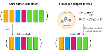
Figure 1: Previous semi-numerical methods produce linearly independent ACE descriptors by applying singular value decomposition (SVD) to a larger set of dependent lexicographically ordered descriptor labels $\bm{nl}$. The new permutation-adapted method takes advantage of permutational symmetries and recursion relationships embedded in the generalized Wigner symbols to define unique basis functions a priori, allowing direct construction of a linearly independent RPI ACE basis.

The set of ACE descriptors in Eq. (6) is poorly conditioned for SVD due to self-interactions.Dusson et al. (2022) This poses a problem for some semi-numerical approaches to ACE using SVD, as it may not be numerically stable for very large $N$ and polynomial degree. However, one compelling feature of ACE models is the ability to generalize to arbitrarily large body order with varying degrees of radial and angular character.Drautz (2019) It is therefore desirable to define systematic approaches for ACE with large $N$ and polynomial degree. In some cases, as we will show in this work, retaining a small number of high body-order interactions can help reduce error in models. Semi-numerical methods can produce sets of ACE descriptors that are adequate for many practical applications.Lysogorskiy et al. (2021); Bochkarev et al. (2022) However, these approaches may not be stable for arbitrarily large body-order, and testing for such cases is difficult and possibly prohibitively expensive.Dusson et al. (2022) Symmetrized bases of atomic environment descriptors possessing either permutational invariance (PI) or rotationally invariance/equivariance (RI), independently have already been constructed.Braams and Bowman (2009); Drautz (2019); Yutsis et al. (1962) To our knowledge, the completeness and independence of the ACE basis remains to be analytically shown. The definition of one would avoid extra numerical steps to construct the ACE basis.

In this work, the properties of the generalized Wigner symbols are used to generate a complete set of independent ACE descriptors. In our method, we consider all possible unique permutations of basis function labels indexed on $\bm{nlL}$. In this permutation-adapted (PA) method; more permutations than ordered $\bm{nl}$ are considered due to the intermediate angular momentum quantum numbers. The method relies on the permutation symmetries of the generalized Wigner symbols as well as raising and lowering operations for the generalized Wigner symbols to obtain a set of independent basis functions. Independence of the basis functions is obtained through two key steps. The first is the construction of complete binary trees out of $\bm{nlL}$ indices and sorting them to avoid obvious repeats $\bm{nl}$ that lexicographical ordering normally resolves. More importantly, it does so while eliminating redundant functions that differ only by a permutation of intermediates. This is not accounted for directly in other methods and functions that are linearly related because their intermediates are just permutations of others are removed using SVD. The second step uses ladder relationships, relationships between multiple basis functions with different intermediates, to obtain a complete set of independent functions. These relationships and extensive background for deriving them is highlighted this work. A key result of this work is a practical methodology for constructing a complete and analytically independent set of ACE descriptors.

III Methodology

III.1 Rotationally Invariant Descriptors

III.1.1 Wigner symbol background

Before starting the construction of this angular basis, we will introduce the Wigner symbols. The angular basis for ACE is a product of $N$ spherical harmonics, one for each bond. The generalized Wigner symbols allow one to reduce a product of spherical harmonics to one spherical harmonic. This process may also be referred to as angular momentum coupling. The fact that this is analogous to coupling quantum angular momenta is a key connection that helps prove linear independence of descriptors in later sections. In the construction of the angular basis for ACE in many practical applications, we need to ensure that the product of $N$ spherical harmonics is rotationally invariant. In short, this will be done by reducing the product of $N$ spherical harmonics to a single spherical harmonic with angular momentum and projection quantum numbers both equal to zero, $Y_{0}^{0}$. This $Y_{0}^{0}$ function is rotationally invariant. We begin this introduction with the traditional Wigner-3j symbols. The traditional Wigner-3j symbols that are used reduce the product of two spherical harmonics to another. In symbolic and matrix form, the traditional Wigner-3j symbols are:

$$W^{l_{3},m_{3}}_{l_{1},m_{1},l_{2},m_{2}}=\begin{pmatrix}l_{1}&l_{2}&l_{3}\\ m_{1}&m_{2}&m_{3}\end{pmatrix}.$$ (7)

Explicit algebraic forms for Eqs. (36) and (37) may be found elsewhere.Wigner (2012); Yutsis et al. (1962) For non-zero traditional Wigner-3j symbols, the triangle condition must be obeyed, $\triangle[l_{1},l_{2},l_{3}]=|l_{1}-l_{2}|\leq l_{3}\leq(l_{1}+l_{2})$. Additionally, there are also conditions on the $m_{i}$. For non-zero Wigner-3j symbols, we must have $m_{1}+m_{2}+m_{3}=0$. As shown in Eq. (38), traditional Wigner-3j symbols are equivalent under permutations of $(l_{i},m_{i})$ tuples (columns in matrix form). It is also convenient to express this Wigner-3j symbol in Eq. (7) as a binary tree, and we will refer to these within, as coupling trees.Yutsis et al. (1962)

This coupling tree structure helps illustrate how the traditional Wigner-3j symbols are used to couple two spherical harmonics. Additionally it provides a simple graphical way to show which permutations of $l_{i}$ yield equivalent Wigner symbols. If one were to permute the two children, switching $l_{1}$ and $l_{2}$, the Wigner-3j symbols would remain unchanged. To couple more than two, the generalized Wigner symbols are used. The generalized Wigner symbols are contractions of multiple Wigner-3j symbols. These are constructed such that $N$ spherical harmonics coupled two at a time until only one remains.

There are multiple ways to construct the generalized Wigner symbols and notation can be challenging. There is some ambiguity in how the $N$ spherical harmonics are coupled; the order in which they are coupled is arbitrary. One example of this arbitrary order of reduction for four spherical harmonics is analogous to adding angular momenta to form an intermediate, $l_{1}+l_{2}\rightarrow L_{1}$, and again for the next two, $l_{3}+l_{4}\rightarrow L_{2}$ then coupling the intermediates to the reduced spherical harmonic with angular momentum and projection, $L_{R},M_{R}$. The corresponding generalized Wigner symbol in matrix form is,

$$\begin{split}&\begin{pmatrix}l_{1}&l_{2}&l_{3}&l_{4}\\ m_{1}&m_{2}&m_{3}&m_{4}\end{pmatrix}=\\ &\sum_{M_{1},M_{2}}\phi(L_{k},M_{k})\begin{pmatrix}l_{1}&l_{2}&L_{1}\\ m_{1}&m_{2}&-M_{1}\end{pmatrix}\begin{pmatrix}l_{3}&l_{4}&L_{2}\\ m_{3}&m_{4}&-M_{2}\end{pmatrix}\\ &\begin{pmatrix}L_{1}&L_{2}&L_{R}\\ M_{1}&M_{2}&-M_{R}\end{pmatrix}\end{split}$$ (8)

where $\phi(L_{k},M_{k})=\prod_{k}(-1)^{L_{k}-M_{k}}$. Another valid generalized Wigner symbol could be constructed by coupling of $l_{1}+l_{2}=L_{12}$, then $l_{3}+L_{12}=L_{123}$, and finally $l_{4}+L_{123}=L_{R}$. As one can see, there are many others. Generalized Wigner symbols constructed with different coupling schemes are not equivalent in general, but are related by some linear transformation.Yutsis et al. (1962) A coupling scheme will often be denoted with a permutation, $\sigma_{c}$, of leaves and/or a binary tree.Yutsis et al. (1962); Drautz (2020); Bochkarev et al. (2022) We will refer to this as the coupling permutation or coupling scheme; the permutation itself describes the order in which spherical harmonics are reduced. For any coupling scheme, the intermediates must obey the proper triangle conditions for constituent Wigner symbols. For Eq. (8), they are $\triangle[l_{1},l_{2},L_{1}]$, $\triangle[l_{3},l_{4},L_{2}]$, and $\triangle[L_{1},L_{2},L_{R}]$. These conditions restrict the intermediate angular momenta $L_{1},L_{2}$. When represented as a binary tree, the coupling scheme is given by the structure of the tree. The $l_{i}$ form the leaves of the tree while the $L_{k}$ are the internal nodes. Some examples are given in Fig. 2.

To avoid ambiguity, we will always reduce the products of $N$ spherical harmonics using a coupling permutation $\sigma_{c}$ that is constructed by coupling disjoint pairs of $l_{i}$. This family of pairwise coupling permutations are characterized by the partition of $S_{N}$ below.

$$\bm{\lambda}_{c}=\begin{cases}N\;even:(2\,,\,2\,,\,2\,\cdots 2(N/2))\\ N\;odd:(2\,,\,2\,,\,2\,\cdots 2(N-1/2)\,,\,1)\\ \end{cases}$$ (9)

Any permutation element of $S_{N}$ that belongs to this partition could be used, so for simplicity, the coupling permutation used will always be the one associated with ordered disjoint cycles from the partition in Eq. (9). In cyclic form, the pairwise coupling permutation is given in Eq. (10).

$$\sigma_{c}=\begin{cases}N=4:\;\;(1,2)(3,4)\\ N=5:\;\;(1,2)(3,4)(5)\\ N=6:\;\;(1,2)(3,4)(5,6)\\ N=7:\;\;(1,2)(3,4)(5,6)(7)\\ \cdots\end{cases}$$ (10)

We will refer to this as the pairwise coupling scheme. The coupling permutations from Eq. (10) result in coupling trees that are complete binary trees where the leaves have values that are angular momentum quantum numbers, $l_{i}$, and the internal nodes have values that are the intermediate angular momenta, $L_{k}$. The coupling trees in our scheme will have a height given simply by the number of internal nodes, $K$, and the number of leaves, $N$.

$$h={\rm{log}}_{2}(K+N+2)\,-\,1$$ (11)

Therefore, a generalized Wigner symbol will be written from here on, using the coupling scheme from Eq. (10), without ambiguity as,

$$\begin{pmatrix}l_{1}&l_{2}&\cdots&l_{N}\\ m_{1}&m_{2}&\cdots&m_{N}\end{pmatrix}^{\sigma_{c}}_{L_{R},M_{R}}({\bm{L}}),$$ (12)

where the coupling permutation, $\sigma_{c}$ will often not be expressed because we define it above, and $L_{R},M_{R}$ will both be zero unless otherwise specified. The generalized Wigner symbols will often be given in a non-matrix form in terms of vectors of angular momentum, projection, and intermediate angular momentum quantum numbers, $\bm{l}=(l_{1}l_{2}\cdots l_{N})$, $\bm{m}=(m_{1}m_{2}\cdots m_{N})$, and $\bm{l}=(L_{1}L_{2}\cdots L_{(N-2)})$, respectively.

$$W_{\bm{l}}^{\bm{m}}(\bm{L}).$$ (13)

The root node values, $L_{R}$ and $M_{R}$, are taken to be zero in this non-matrix form. An alternative form for the generalized Wigner symbols would be in the form of a complete binary tree with height from Eq. (11). Note that for non-zero generalized Wigner symbols, the triangle conditions must be obeyed for the $N-2$ intermediates indexed on $k$ and all children. The collections of triangle conditions for generalized Wigner symbols are sometimes referred to as the polygon conditions.Yutsis et al. (1962) All triangle conditions for the generalized Wigner symbols in the pairwise coupling scheme may

$$\begin{split}\triangle[C_{1},C_{2},P]=\\ |C_{1}-C_{2}|\leq P\leq C_{1}+C_{2}\end{split}$$ (14)

where the two children for the parent node, $P$ are denoted by $C_{1}$ and $C_{2}$. As an example, the way one of these triangle conditions is formed at the lowest level for $L_{R}$, Eq. (14) will lead to $\triangle[L_{(N-3)},L_{(N-2)},L_{R}]$. The set of intermediate vectors that obey all triangle conditions in Eq. (14) may be referred to as $\{\bm{L}\}_{L_{R}}$. At this stage, we have defined specifically which generalized Wigner symbols we will use, what form they take in symbolic, matrix, and tree forms. We have additionally defined the values that the intermediate angular momentum quantum numbers may take, along with the set of intermediate vectors obeying polygon conditions. Additional properties of the generalized Wigner symbols, specifically those that are important for the construction of the permutation-adapted basis, will be discussed later.

III.1.2 Angular basis

The angular portion of the ACE basis is a product of $N$ spherical harmonics, and is related to a product of $N$ irreducible representations of $SO(3)$. In general, the product is reducible. The construction of a rotationally invariant basis that spans this space is known.Yutsis et al. (1962); Dusson et al. (2022) There are multiple ways to construct a basis that spans this space, but some key equations from previous works give important information such as the basis size. Equation (15) is given to provide the result from other works that yields the size of the basis. We will make reference to this in later sections. The matrix $\mathbf{C}_{\bm{l}}$ may be used to reduce the products of $N$ representations of SO(3), $D_{l_{i}}$, to a sum of irreducible representations of SO(3), $D_{L_{R}}$.Yutsis et al. (1962); Fulton and Harris (2013)

$$\mathbf{C}_{\bm{l}}^{-1}D_{l_{1}}\times D_{l_{2}}\times\cdots D_{l_{N}}\mathbf{C}_{\bm{l}}=\sum_{R(\bm{L})}\alpha_{R}D_{L_{R}}$$ (15)

Following the form of Ref. [​3], $\alpha_{R}$ is the multiplicity of the irreducible representation with value, $L_{R}$. It is easy to show that $\alpha_{R}$ is given by the number of valid sets of intermediates (the size of $\{\bm{L}\}_{L_{R}}$). The elements of the matrix, $\mathbf{C}_{\bm{l}}$ are the generalized Clebsch-Gordan coefficients. Equivalently, the generalized Wigner symbols, $\mathbf{W}_{\bm{l}}$, may be used along with some conversion factors for the same effect.Yutsis et al. (1962) From here on, the generalized Wigner symbols will be used rather than the generalized Clebsch-Gordan coefficients due to convenient permutation properties. The use of generalized Wigner symbols is not required for our method; they just offer convenient properties.

To construct a complete basis (not necessarily rotationally invariant) that spans the space that the irreducible representations on the right hand side of Eq. (15). For each $D_{L_{R}}$, we must have a basis function for each dimension of $D_{L_{R}}$. It is known that the dimension of a given irreducible representation of SO(3), $D_{l}$ is given by $d=2l+1$.Yutsis et al. (1962) From 7.4 of Yutsis, we have the more general expression that gives the dimension of the product in the left hand side of Eq. (15).

$$\prod_{i}^{N}(2l_{i}+1)=\sum_{L_{R}}\alpha_{R}(2L_{R}+1)$$ (16)

This gives the dimension of basis we need to make a basis spanning the space each $D_{L_{R}}$ does. More simply, one may take advantage of the fact that the family of spherical spherical harmonics with a given angular momentum state, $L_{R}$, act as complete and orthonormal basis for the irreducible representation of SO(3), $D_{L_{R}}$.

The spherical harmonic basis with angular momentum quantum numbers $L_{R}$ can be decomposed into sums of products of spherical harmonics by using the generalized Wigner symbols. As a result, we may write a basis function as below.Yutsis et al. (1962)

$$V_{\bm{l},M_{R}}^{\bm{L},L_{R}}=\sum_{\bm{m}\rightarrow M_{R}}W_{m_{1}m_{2}\cdots m_{N}}^{l_{1}l_{2}\cdots l_{N}}(\bm{L})Y_{l_{1}}^{m_{1}}Y_{l_{1}}^{m_{1}}\cdots Y_{l_{N}}^{m_{N}}$$ (17)

We will notice immediately that due to Eq. (16), that the family of functions (all possible $M_{R}$) in this equation above has can span the space that our irreducible representations of SO(3) do, provided that we can calculate $\alpha_{R}$. The generalized Wigner symbols depend on the set of intermediate angular momentum quantum numbers, $\bm{L}$, that are used to couple the $N$ spherical harmonics. Only some sets of intermediates are valid, and all others make the generalized Wigner symbols zero. These sets of valid intermediates obey polygon conditions, which are just repeatedly applied triangle conditions for each coupled $l_{i},l_{j},l_{k}$. The number of sets of valid intermediates is equal to $\alpha_{R}$. To obtain a complete basis, one needs to define the basis functions as in Eq. (17) for all valid sets of intermediates.

For the purposes of this work, cases of rotationally invariant (RI) functions will be considered. In other words, we will only concern ourselves with the functions for $L_{R}=0$. These RI functions will be written as,

$$b_{\bm{l}}^{\bm{L}}=\sum_{\bm{m}}W_{m_{1}m_{2}\cdots m_{N}}^{l_{1}l_{2}\cdots l_{N}}(\bm{L})Y_{l_{1}}^{m_{1}}Y_{l_{1}}^{m_{1}}\cdots Y_{l_{N}}^{m_{N}}$$ (18)

where the sum is taken over all possible collections of $-l_{i}\leq m_{i}\leq l_{i}$ such that $\sum_{i}{m_{i}}=0$, which is the only allowed projection for $M_{R}$. The functions from Eq. (18) are the functions from the more general case in Eq. (17), but for $L_{R}=0$. For this reason, the specific value of $L_{R}$ and $M_{R}$ are omitted; it is implied that they are zero. Completeness and orthogonality of the functions in Eq. (18) follow from completeness and orthogonality of the generalized Wigner symbols.Yutsis et al. (1962) However, the construction of RI basis functions in practical applications of ACE involves building descriptors that are symmetric with respect to permutations as well.

To begin the construction of rotation and permutation invariant functions, one may start by doing exactly that in $\eqref{eq:ri_product}$, but on angular functions that have been made invariant with respect to permutations, now indicated by a bar in Eq. (19).

$$\tilde{b}_{\bm{l}}^{\bm{L}}=\sum_{\bm{m}}W_{\bm{l}}^{\bm{m}}(\bm{L})\bar{\bm{Y}}_{\bm{m}}^{\bm{l}}$$ (19)

Symmetrizing angular functions inside the sum with respect to permutations is straightforward to do.Dusson et al. (2022) This does introduce linear dependencies between functions when some $l_{i}$ and/or $L$ are duplicates of others. This means that the set of RPI angular functions constructed by Eq. (19) is overcomplete. Investigating these linear dependencies is one key focus of this work. We find that they arise from the permutation symmetries of the generalized Wigner symbols, recursion relationships, and the fact that the angular basis is now also symmetric with respect to permutations.

III.1.3 Properties and Linear Dependence

While the choice of the coupling scheme for the generalized Wigner symbols, $\sigma_{c}$, is an arbitrary one, one may notice that certain coupling schemes allow for more equivalent permutations of leaves than others. This is easier to see graphically. This is highlighted in the tree diagram in Fig. 2. The first scheme in Fig. 2 is the pairwise coupling scheme used in Eq. (8). Permutations of children, of a parent (e.g. permuting $l_{1}$ and $l_{2}$) the generalized Wigner symbol remains unchanged based on Eq. (38). Similarly, permutations of branches are equivalent as well; permuting $L_{1}$ and $L_{2}$ and all corresponding children gives an equivalent generalized Wigner symbol. The second scheme, though amenable to recursive evaluation algorithms,Dusson et al. (2022) has more complicated permutation properties. The permutation symmetries of the generalized Wigner symbols have not yet been reported in detail, so we provide the thorough background, demonstrations, and proofs of these symmetries in Appendix A and to a lesser extent in later sections. To summarize the outcome of these permutation symmetries: equivalent permutations of leaves and or intermediates of a generalized Wigner symbol result from permutations equivalent permutations of Wigner 3-j symbols, c.f. Eq. (38) and Eq. (39).

(a)

(b)

Figure 2: Two tree diagrams for generalized Wigner symbols of rank 4. Both (a) and (b) represent valid coupling schemes. The indices that are symmetric as a result of Eq. (38) are highlighted in corresponding colors. The coupling scheme in (a) preserves permutation symmetry in more of the $(l_{i},m_{i})$ tuples, rather than in the intermediates $L_{k}$. Scheme (a) was used to couple Clebsch-Gordan coefficients in Ref. [​18]. Scheme (b) was used to couple Clebsch-Gordan coefficients in Ref. [​19].

In the pairwise coupling scheme, Eqs. (9) - (10), the transpositions of any two coupled indices (e.g. $l_{1}$, $l_{2}$ children of $L_{1}$) are equivalent through Eq. (38). In practice, there are more elegant and efficient ways to construct all equivalent permutations of generalized Wigner symbols through methods such as Young subgroup fillings of $S_{K+N}$ and/or construction of more general automorphism groups that have been defined for complete binary trees using wreath products of $S_{2}$.James (2006); Knuth (1970); Brunner and Sidki (1997) Some of these methods are highlighted in Appendix A, but for the purposes of demonstrating where the permutation symmetries come from, we will construct the set of equivalent permutations by applying Eq. (38) for every coupled pair of angular momentum quantum numbers in a generalized Wigner symbol. It is straightforward to collect and combine all of these transposition permutations. In rank 4 symbol example, equivalent transposition permutations for each the coupled sets of indices are:

$$\begin{cases}T_{(l_{1},l_{2})}:[(),(12)]\\ T_{(l_{3},l_{4})}:[(),(34)]\\ T_{(L_{1},L_{2})}:[(),(56)]\end{cases}$$ (20)

where $(56)$ corresponds to a transposition of the two intermediate angular momenta, $L_{1}$ and $L_{2}$ and the blank cycles are the identity permutations for each pair. Taking all possible combinations of permutations (the direct product of the subsets) in Eq. (20) yields:

$$\begin{split}&T_{4}=\{(),(12),(12)(34),\\ &(12)(34)(56),(12)(56),(34),(34)(56),(56)\}\end{split}$$ (21a)

$$\begin{split}&G_{4}=\{(),(12),(12)(34),\\ &(14)(23),(1324),(34),(1423),(13)(24)\}\end{split}$$ (21b)

where $G_{4}$ is obtained by rewriting elements of $T_{4}$ that contain intermediate indices (56) in terms of their action on their children. As was done for rank 4 in Eq. (20), we may use Eq. (38) to generate equivalent transpositions for all coupled indices in a rank $N$ Wigner symbol.

$$\begin{cases}T_{(l_{1},l_{2})}:[(),(12)]\\ T_{(l_{3},l_{4})}:[(),(34)]\\ \cdots\\ T_{(l_{N-1},l_{N})}:[(),(N-1,N)]\\ T_{(L_{1},L_{2})}:[(),(N+1,N+2)]\\ \cdots\\ T_{(L_{N-3},L_{N-2})}:[(),(N+K-1,N+K)]\\ \end{cases}$$ (22)

From Eq. (22), the set of all equivalent permutations, $T_{N}$, may be generated by taking the direct product of all subsets of equivalent transpositions. In Eq. (22), there are now transpositions for all $N/2$ coupled angular momentum quantum numbers as well as for all $N-2$ intermediate angular momentum quantum numbers. To obtain $G_{N}$, the transpositions of internal nodes may be written in terms of their action on leaf nodes.

In addition to the group of permutation automorphisms, generalized Wigner symbols may be related to others using recursion relationships. These recursion relationships follow from applying ladder operators used to raise/lower quantum mechanical angular momentum states.Rose (1995) The recursion relationships for the generalized Wigner symbols have yet to be derived, but it is straightforward to do so by iteratively applying raising/lowering operations to the traditional Wigner-3j symbols that comprise the generalized Wigner symbol. Derivations for these are provided in Appendix B, but we will list some key relationships here. The first set of relationships relate generalized coupling coefficients with some initial vector of intermediates $\bm{L}$ to another with intermediates that have been incremented, $\bm{L}+\bm{k}$, while $\bm{lm}$ remain fixed. This may be derived for arbitrary rank $N$ couplings with intermediates that have been incremented by integer values $k_{i}\cdots k_{N-2}$ times, as reported in Appendix B. For the sake of brevity here, it is given for rank 4 only and the case of $L_{R}=0$.

$$\begin{split}&\begin{pmatrix}l_{1}&l_{2}&l_{3}&l_{4}\\ m_{1}&m_{2}&m_{3}&m_{4}\end{pmatrix}\big{(}L_{1},L_{2},L_{R}=0\big{)}=\\ &A_{-,-}(\bm{l},\bm{m})\begin{pmatrix}l_{1}&l_{2}&l_{3}&l_{4}\\ m_{1}&m_{2}&m_{3}&m_{4}\end{pmatrix}\big{(}L_{1}-1,L_{2}-1,L_{R}=0\big{)}\\ &+\\ &A_{+,+}(\bm{l},\bm{m})\begin{pmatrix}l_{1}&l_{2}&l_{3}&l_{4}\\ m_{1}&m_{2}&m_{3}&m_{4}\end{pmatrix}\big{(}L_{1}+1,L_{2}+1,L_{R}=0\big{)}\end{split}$$ (23)

In Eq. (23), we provide exact expressions for generalized Wigner symbols with incremented intermediates. The constants, $A_{\pm,\pm}$ follow from Eq. (47), and may be written entirely in terms of $l_{i}$ and $m_{i}$. The result is that generalized Wigner symbols with some specific $\bm{L}$ may be related to those with different intermediates $\bm{L}^{\prime}$.

The second set of relationships that are used in the derivation of the PA method relates coupling coefficients with fixed $\bm{lL}$ and one set of projection quantum numbers, $\bm{m}$, to those with another set of projection quantum numbers, $\bm{m}^{\prime}$. Similar to the raising/lowering operations for angular momentum quantum numbers, these are derived by iteratively applying raising/lowering operations for traditional Wigner-3j symbols. Additionally, these can also be derived for arbitrary coupling rank as seen in Appendix B. For brevity again, the rank 4 case is given.

$$\begin{split}&\begin{pmatrix}l_{1}&l_{2}&l_{3}&l_{4}\\ m_{1}&m_{2}&m_{3}&m_{4}\end{pmatrix}\big{(}\{M_{1}\pm 1,M_{2}\mp 1\},M_{R}\big{)}\\ &=\sum_{\bm{\mathcal{M}}}c_{\bm{\mathcal{M}}}(\bm{l},\bm{m})\begin{pmatrix}l_{1}&l_{2}&l_{3}&l_{4}\\ m_{1}^{\prime}&m_{2}^{\prime}&m_{3}^{\prime}&m_{4}^{\prime}\end{pmatrix}\big{(}\{M_{1},M_{2}\},M_{R}\big{)}\end{split}$$ (24)

In Eq. (24), $\bm{M}=\{M_{1}\pm 1,M_{2}\mp 1\}$ is incremented such that $M_{R}$ is conserved. Raising and lowering the $m_{i}$ to do so relates the Wigner symbol to other Wigner symbols with $\bm{\mathcal{M}}=(M_{1},M_{2})$. The set of related coefficients is written explicitly in Eq. (65). The coefficients, $c_{\bm{\mathcal{M}}}(\bm{l},\bm{m})$ follow from generalizing Eqs. (54) - (56). It is worthwhile to note that for important practical cases such as when $l_{1}=l_{2}=l_{3}=l_{4}$ and constant $|M_{k}|$, the $c_{\bm{\mathcal{M}}}(\bm{l},\bm{m})$ are often the same. This allows one to combine many terms in Eq. (6), and derive relationships between functions when they have different intermediates, $\bm{L}\neq\bm{L}^{\prime}$. Both the equivalent permutations from $G_{N}$ as well as the generalized recursion relationships, Eq. (23) and Eq. (24), are used to derive exact relationships between rotation and permutation invariant functions. For example, using the relationships derived within for equivalent permutations of Wigner symbols and generalized relationships, we prove in Appendix B, relationships such as

$$\bar{b}_{(1111)(22)}=\frac{2}{5\sqrt{5}}\bar{b}_{(1111)(00)},$$ (25)

which can be verified numerically. These may be derived for all possible values of intermediates and extended to other values of angular momentum quantum numbers. Doing so provides relationships between descriptors that have the same number of duplicate angular momentum quantum numbers and the same number of duplicate intermediate quantum numbers. We refer to these relationships as ladder relationships, and they may be used to construct a set of linearly independent rotation and permutation invariant (RPI) angular functions. These ladder relationships between basis functions should not be confused with the recursion relationships for angular momentum and projection quantum numbers of the Wigner symbols in Eqs. (23) and (24).

III.1.4 Comparing RI and RPI angular bases

Two versions of the angular basis will be constructed before including a radial component. One will be referred to as the canonical basis (C-RI). The canonical RI basis starts with a fixed, ordered set of $l_{i}$, and is not invariant with respect to permutations, but it is invariant with respect to rotations. The set of vectors of intermediate angular momenta obeying polygon conditions gives the size of the canonical RI basis. This set of intermediate vectors was referred to earlier as $\{\bm{L}\}$. The canonical basis functions may be indexed on the fixed $l_{i}$ and corresponding intermediate angular momentum vectors that obey iterated triangle conditions, $\bm{l}\bm{L}$. The function labels for an exhaustive list of $\bm{l}$ up to $l_{max}=3$ is given in Table 1.

The precursor to the second version of the angular basis, is the overcomplete basis generated by the set of all unique permutations of $\bm{l}\bm{L}$. This is just the construction of all functions of the form in Eq. (19), for the unique $\bm{l}$ permutations. This is also overcomplete by construction. This overcomplete PA-RI^∗ basis spans the same space as the canonical basis, but with all unique permutations of $l_{i}$ exposed. Examples are given for this basis in Column 3 of Table 1 and is referred to as PA-RI^∗. This step may seem convoluted or unnecessary, but including extra permutations of $\bm{l}\bm{L}$ is a necessary step to obtain a complete RPI radial and angular basis. Demonstrations of this will be given in the results.

From this overcomplete basis, the permutation-adapted rotation and permutation invariant (PA-RI) basis is constructed. One set of functions must be selected that spans the same space as the canonical one, but redundancies due to the permutation invariance must be eliminated. Additionally, leveraging both the permutation symmetries and recursion relationships for the generalized Wigner symbols allows one to show that subsets of a rotation and permutation invariant basis are dependent. A complete and independent set of PA-RI labels may be defined by selecting only one label from each subset.

III.1.5 Canonical rotation invariant descriptor procedure

The canonical RI procedure is straightforward. Obtaining an RI basis that is not permutation invariant has been done.Dusson et al. (2022) For all sorted vectors of angular momentum quantum numbers, the sets of intermediate angular momenta, $\{\bm{L}\}$, are generated. The canonical RI basis functions are all those indexed on sorted angular momentum quantum numbers and corresponding intermediates, $\bm{l}\bm{L}$. Simply put, these are the functions of the form in Eq. (18). Note again that these are not invariant with respect to permutations.

III.1.6 Permutation-adapted rotation and permutation invariant procedure

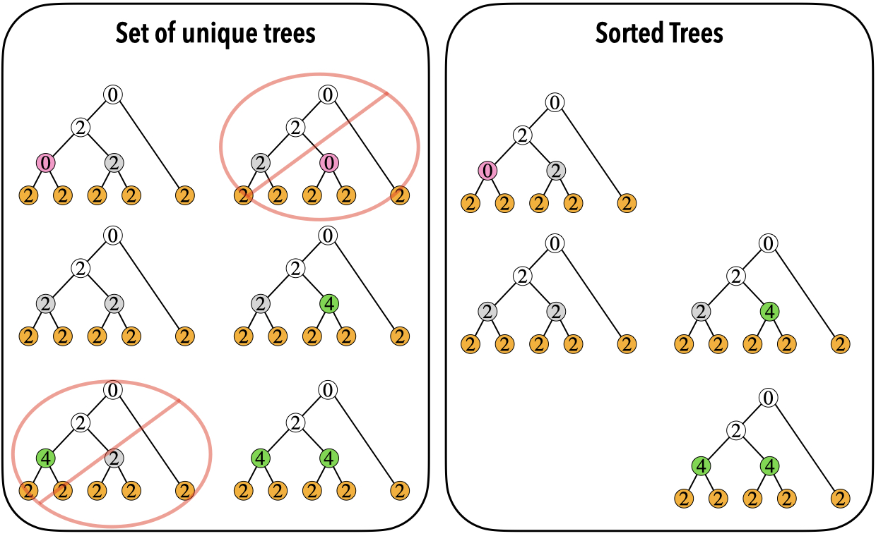
(a)

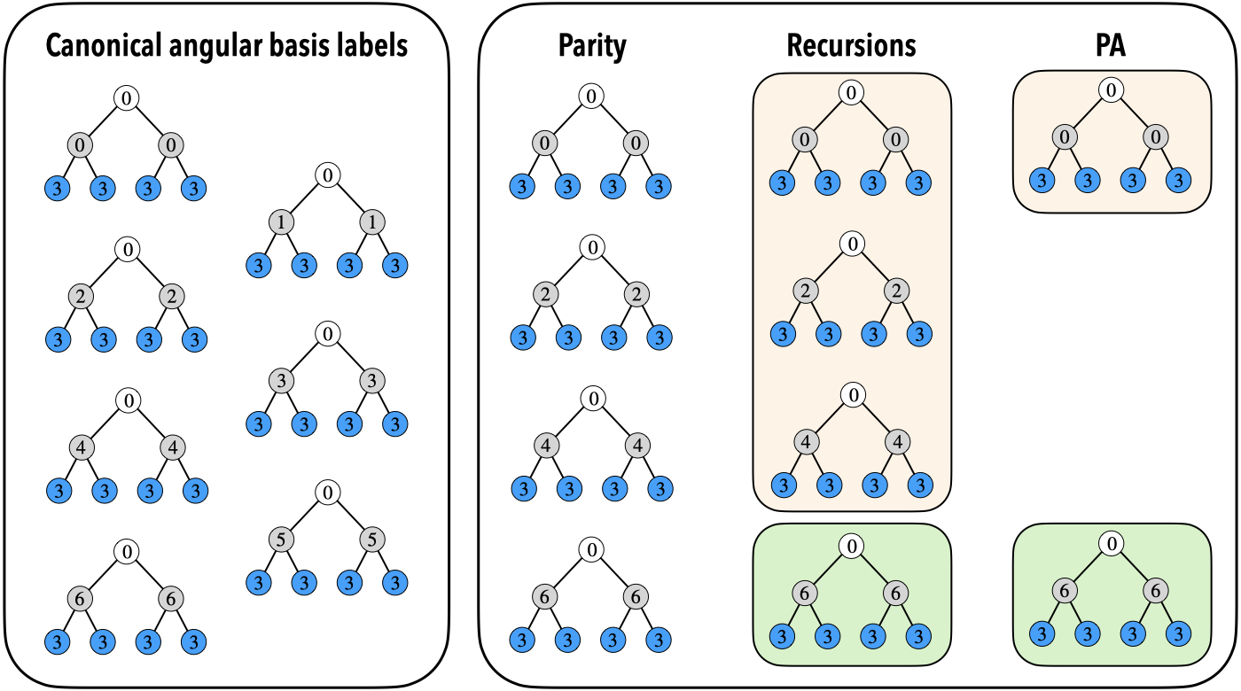
(b)

Figure 3: The diagram in (a) shows how, for the example of $\bm{l}=(22222)$, generating expanded sets of labels, organizing them in coupling trees, and applying tree sorting, one may eliminate labels that are equivalent by permutation. In (b), the result of applying intermediate ladder relationships for functions with incremented intermediates, Appendix B, is shown for a rank 4 descriptor with $\bm{l}=(3333)$. Labels that are redundant due to raising/lowering of intermediates are eliminated with this step.

To construct the PA-RI basis, we begin the same way as with the canonical RI basis. A key difference is that it may be repeated for some permutations of angular momentum quantum numbers as well. In the most general cases, multiple permutations of angular momentum quantum numbers must be considered to obtain a complete rotation and permutation invariant basis. Using multiple permutations of $\bm{l}\bm{L}$ in the construction of a basis can be done because any two coupling schemes are related to one another by a linear transformation, however it will be overcomplete. For a given set of angular momentum quantum numbers, a set of intermediates is generated based on generalized triangle conditions, $\{\bm{L}\}^{\varsigma}$ where $\varsigma$ denotes the permutation of $\bm{l}$ used to generate the intermediates. For the PA-RI basis, parity constraints are also enforced on the angular momentum quantum numbers and the intermediates, $\sum_{i}l_{i}\;:\;{\rm{even}}$.

$$\begin{split}&\sum_{i}l_{i}\;:\;{\rm{even}}\\ &\{(C_{1}+C_{2}+P_{1})\;:\;{\rm{even}}\}\forall(C_{i},C_{j},P_{k})\in\bm{lL}\end{split}$$ (26)

In Eq. (26), the first condition is applied to all angular momentum quantum numbers (leaves). The second set of constraints is applied to all parent-children combinations in $\bm{lL}$ when it is constructed as a binary tree. For example, a block of 4-bond RPI angular functions may yield a set of labels, $\{\bm{lL}\}=\{(1111)(00),(1111)(11),(1111)(22)\}$. The second $\bm{lL}=(1111)(11)$ is eliminated because it does not obey $(C_{1}+C_{2}+P_{1})\;:\;{\rm{even}}$. Not only does enforcing these parity constraints ensure that the RPI angular functions obey inversion symmetry, it also eliminates RPI functions that would zero-valued in our pairwise coupling scheme. This alone is not enough to eliminate all redundant functions though, and the RPI angular basis at this stage is still overcomplete. This overcomplete set of functions can be reduced to a complete and independent basis if the relationships between dependent functions are known.

Linear dependence between angular RPI functions typically arises in two different ways. The first is that permutations of intermediates that yield an equivalent coupling tree give equivalent basis functions. This can remedied by sorting binary coupling trees as in Fig. 3 (a). The second are linear dependencies and cancellations between the sets of intermediates. The result of ladder relationships and parity constraints are highlighted in Fig. 3 (b). Here, we note again that there is a distinction between ladder relationships of functions the recursion relationships of the generalized Wigner symbols. The recursion relationships of the generalized Wigner symbols are used to derive the other, but they are not the same. When all subsets of linearly dependent functions are known, a set of linearly independent functions may be selected that may or may not contain multiple permutations of angular momentum quantum numbers. This is at the core of the PA-RI (and the PA-RPI) method. The permutation-adapted method may be summarized in two steps that address the two key sources of linear dependence listed above. All functions related by some permutation are eliminated. Subsets of linearly dependent functions are exposed in the overcomplete set, and only one function from each dependent subset is used to construct a complete and independent set. We describe how each step is performed in more technical detail.

The first step in the permutation-adapted approach is to obtain all unique $\bm{l}\bm{L}$ labels up to automorphism. In general, the unique permutations of $\bm{l}\bm{L}$ may be found by constructing a sorted, complete binary tree for each permutation of $\bm{l}\bm{L}$ where the $l_{i}$ are the leaf nodes and $L_{k}$ are the internal nodes. These binary trees may then be compared against elements of $G_{N}$ and collecting only the unique ones. While straightforward, this approach can be expensive. This is especially true for large body-order functions. In practice, this can be done using semi-standard Young tableau fillings.Fomin (1988); Schensted (1961) The correspondence between permutations and Young Tableu fillings allows one to consider a subset of permutations rather than all possible permutations. This provides all permutations $\bm{lL}$ that are needed to construct the unique basis labels. There are cases, such as when $\bm{l}=(22222)$, that a set of intermediates generated by triangle conditions is just a permutation of another set of intermediates. Functions with such labels are eliminated because they do not correspond to a sorted binary tree. The graphic in Fig. 3 (a) demonstrates how this is done.

The next step in the angular PA-RI procedure reduces the basis labels based on relationships between functions with different intermediates. The ladder relationships between basis functions depend on how many $\bm{l}$ and/or $\bm{L}$ are equivalent as well as the rank $N$. Some ladder relationships are derived in Appendix B, and we highlight archetypal cases to show how they may be derived instead of giving them for all possible degeneracies of $\bm{l}$, $\bm{L}$, and rank. However, the recursion relationships for the generalized Wigner symbols of arbitrary rank are derived and given in Eq. (69); these may be used to derive more general ladder relationships between basis functions. These relationships are applied to the unique $\bm{l}\bm{L}$ trees generated from the first step. This exposes subsets of dependent functions with incremented indices, $\bm{l}\bm{L}_{\pm(1),\pm(2),\cdots\pm(N-2)}$, for all intermediates. A complete and independent set of PA-RI labels may be defined by selecting one function from each dependent subset.

Therefor, a complete set of independent rotation and permutation invariant angular descriptors is characterized by a set of binary trees that are unique up to permutations and ladder relationships. A comparison between the canonical RI basis, the overcomplete set generated by the unique permutations of $l_{i}$, and the reduced (independent) of PA-RI labels are given in Table 1. Pseudocode for this procedure closely follows that for the case where a radial component is included in the basis and is given in the next section.

	C-RI	RI∗	PA-RI
$\sigma_{\circ}(\bm{l})$	$\sigma_{\circ}(\bm{l})\bm{L}$	$\varsigma(\bm{l})\bm{L}^{*}$	$\varsigma(\bm{l})\bm{L}$
(1111)	$(1111)(00)$ $(1111)(11)$ $(1111)(22)$	$(1111)(00)$ $(1111)(22)$	$(1111)(00)$
(1113)	$(1113)(22)$	$(1113)(22)$	$(1113)(22)$
(1122)	$(1122)(00)$ $(1122)(11)$ $(1122)(22)$	$(1122)(00)$ $(1122)(22)$ $(1212)(11)$ $(1212)(33)$	$(1122)(00)$ $(1212)(11)$
(1133)	$(1133)(00)$ $(1133)(11)$ $(1133)(22)$	$(1133)(00)$ $(1133)(22)$ $(1313)(22)$ $(1313)(44)$	$(1133)(00)$ $(1313)(22)$
(1223)	$(1223)(11)$ $(1223)(22)$ $(1223)(33)$	$(1322)(22)$ $(1322)(44)$ $(1223)(11)$ $(1223)(33)$	$(1223)(11)$ $(1223)(33)$
(1333)	$(1333)(22)$ $(1333)(33)$ $(1333)(44)$	$(1333)(22)$ $(1333)(44)$	$(1333)(22)$
(2222)	$(2222)(00)$ $(2222)(11)$ $(2222)(22)$ $(2222)(33)$ $(2222)(44)$	$(2222)(00)$ $(2222)(22)$ $(2222)(44)$	$(2222)(00)$
(2233)	$(2233)(00)$ $(2233)(11)$ $(2233)(22)$ $(2233)(33)$ $(2233)(44)$	$(2233)(00)$ $(2233)(22)$ $(2233)(44)$ $(2323)(11)$ $(2323)(33)$ $(2323)(55)$	$(2233)(00)$ $(2233)(22)$ $(2323)(11)$
(3333)	$(3333)(00)$ $(3333)(11)$ $(3333)(22)$ $(3333)(33)$ $(3333)(44)$ $(3333)(55)$ $(3333)(66)$	$(3333)(00)$ $(3333)(22)$ $(3333)(44)$ $(3333)(66)$	$(3333)(00)$ $(3333)(66)$

Table 1: The full set of RI basis functions for all valid $\sigma_{\circ}(\bm{l})$ up to $l_{max}=3$ and $L_{R}=0$. These collections of valid angular momentum quantum numbers obey $\sum_{i}l_{i}$ even. The canonical RI labels (C-RI) for angular functions without permutation invariance is given in the second column. The superset of permutation invariant RI labels is given in the third column, (RI^∗), and the reduced PA-RI basis labels for permutation invariant angular functions is given in the fourth.

In Table 1, it can be seen that the C-RI and PA-RPI bases are equivalent in some cases. In cases where they are not the same, labels corresponding to dependent functions have been eliminated. The relationships for descriptors with dependent intermediates follow from the recursion relationships in Appendix B between generalized Wigner symbols as well as the permutation symmetries of the generalized Wigner symbols. After applying these ladder relationships we may find the independent angular basis function labels for a permutation-symmetrized angular basis.

III.2 RPI Angular and Radial Basis

We are now interested in eliminating redundant functions in a radial + angular basis that has been symmetrized with respect to rotations and permutations.

$$B_{\bm{nlL}}=\sum_{\bm{m}}W_{\bm{l}}^{\bm{m}}(\bm{L})\bar{\bm{\Phi}}_{\bm{nlm}}(\bm{r})$$ (27)

In Eq. (27), ’cluster basis’ from Eq. (2) has been symmetrized with respect to permutations. It is made rotationally invariant by contracting the permutation invariant cluster basis with the generalized Wigner symbols. Similar to the purely angular basis, the functions defined by Eq. (27) are also over-complete. As PA-RI functions are determined for an angular basis with indices $\bm{lL}$, PA-RPI functions for a radial + angular basis may be determined in a similar way. The permutation symmetries of the coupling tree allows one to generate all unique $\bm{nlL}$ labels up to automorphism as they were for the PA-RI functions. Ladder relationships may be used to eliminate linearly dependent functions with different intermediates with the radial + angular basis as well. These ladder relationships must now be defined for different numbers of duplicate $n_{i}$, $l_{i}$, and $L_{k}$ rather than just angular indices. This is similar to the PA-RI procedure where binary trees are sorted from the leaves, and secondly on intermediates. The difference is that the level of the tree containing the angular momentum indices are appended with the radial indices, $\bm{n}$. A set of radial + angular functions that are unique up to automorphism of the coupling tree are not related by ladder relationships form a complete and independent set of ACE basis functions. The corresponding descriptors will be referred to as the radial + angular PA-RPI descriptors. The size of the PA-RPI basis is intuitively determined by the number of unique $\bm{nlL}$ permutations up to permutation automorphisms and ladder relationships.

In order to construct these labels, the following procedure may be used. First, all $\bm{nl}$ permutations are constructed, and the corresponding intermediates are added according to iterated triangle conditions and parity constraints. The resulting $\bm{nlL}$ labels are constructed as coupling trees, and are sorted from highest levels of the tree (leaves) to lowest levels (intermediates/branches). In pseudocode, this first step is:

$tree\_set$

$nlperms$ = build_nl_perms($\bm{n}_{\circ}$, $\bm{l}_{\circ}$)

for ($\bm{n}$, $\bm{l}$) in nlperms do

     for $\bm{L}$ in generalized_triangle_conditions($\bm{l}$) do

         $tree$ = binary_tree($\bm{n}$, $\bm{l}$, $\bm{L}$)

         $tree\_set\leftarrow tree$

     end for

end for

For the sake of simplicity, the build_nl_perms function can be interpreted as one that generates all permutations of $\bm{n}$ and $\bm{l}$, then the trees are sorted. In practice, there are efficient ways to generate unique permutations only. This first step is shown for only one vector of $\bm{nl}$, and relevant permutations. In practice, step one is repeated for all combinations of radial and angular indices up to some specified $n_{max}$ and $l_{max}$, respectively. The second step is to select a set of $\bm{nlL}$ labels that are not related by permutations or recursion relationships to others. This may be done by with the following procedure.

$PA\_set$

$per\_leaves$ = $tree\_set.per\_nl\_duplicates$

for  $\bm{nl}\_subset$ in $per\_leaves$ do

     $combined\_\bm{nl}=filter\_permutations(\bm{nl}\_subset)$

     $related\_subsets$ = $ladder\_relate(combined\_\bm{nl})$

     $PA\_set\leftarrow select\_per\_subset(related\_subsets)$

end for

The function $per\_nl\_duplicates$ sorts the trees by the number and values of the duplicate of $n_{i}$, $l_{i}$, and $L_{k}$. Ladder relationships are applied to subsets of trees that have the same number and values for duplicate $n_{i}$, $l_{i}$, and $L_{k}$. In the for loop, the $filter\_permutations$ regroups the $\bm{nl}$ permutations (which may have different permutations of $\bm{l}$) and maps them to $\sigma_{\circ}\bm{l})$ trees so that ladder relationships can be applied. Ladder relationships may differ per permutation of $\bm{nl}$. The function $ladder\_relate$ gets the linearly related subsets of functions that share the same number and values for duplicate $n_{i}$, $l_{i}$, and $L_{i}$. It relies on the ladder relationships between RPI functions. This function gives sets of functions with raised/lowered $\bm{L}$ that are linearly related. One function is selected from each subset, $select\_per\_subset$, to form the PA basis. The number of functions that are related by ladder relationships intermediates grow with the number of $n_{i}$, $l_{i}$, and $L_{k}$ duplicates. In some maximum degeneracy cases and for small $l_{i}$, e.g. $\bm{nl}=(1111)(1111)$, only one $\bm{nlL}$ is independent. This is proven in Appendix B and highlighted in the next subsection.

As an important note on cost of step 1 in the procedure, which may involve searches $S_{K+N}$. This could become cumbersome very quickly. Presenting the method a brute-force search over this permutation group is good for pedagogical purposes, but it is not what is done in practice. This is why we emphasize that many of the steps only needs to be done once for a given set of duplicate $\bm{l}$. For example, the construction of unique leaf permutations for $\bm{nl}=(1122)(1122)$ may be applied to $\bm{nl}=(4455)(1122)$ and $\bm{nl}=(4455)(4466)$, etc. Additionally, the approaches we use in practice, such as employing the Robinson-Schensted-Knuth correspondence theorem, allow us to consider Young Subgroup fillings of $\bm{1122}$ rather than all permutations in $S_{N}$.Knuth (1970) At the very most for our rank 4 example above, we would only need to consider $\bm{l}\in\{(1122),(1212),(2211)\}$, or 6 total permutations in the case where all $l_{i}$ are nonequivalent.

III.2.1 Highlighted results and examples

Sorting the angular momentum quantum numbers is not sufficient to produce a complete and independent basis for all coupling schemes. Specifically for the pairwise coupling scheme used within, additional permutations of $\bm{l}$ may be required. An illustrative example within the $\sigma_{c}=(12)(34)$ coupling scheme is $\bm{n}=(1122)$ and $\bm{l}=(1122)$. We show where using lexicographical ordering of $(n_{i},l_{i})$ for this fixed permutation of $\bm{l}$ does not work, and where the PA-RPI method remedies it. Forcing $\bm{nl}$ to be ordered first on $l_{i}$ in $\bm{nl}$ tuples gives

$$\{\bm{nl}\}=\{(1122)(1122)\,,\,(1212)(1122)\,,\,(2211)(1122)\}.$$ (28)

There are two intermediate vectors allowed after parity constraints, $\{\bm{L}\}=\{(00),(22)\}$. The intermediate vector $(11)$ is eliminated for $\bm{l}=(1122)$ due to parity constraints in the $\sigma_{c}=(12)(34)$ coupling scheme. All possible descriptor labels generated by this example, before any reduction due to raising/lowering operations, are given by:

$$\begin{split}&\{\bm{nl}\}\times\{\bm{L}\}=\{(1122)(1122)(00)\,,\,(1212)(1122)(00)\,,\,\\ &(2211)(1122)(00)\,,\,(1122)(1122)(22)\,,\,\\ &(1212)(1122)(22)\,,\,(2211)(1122)(22)\}\end{split}$$ (29)

The problematic result of Eq. (29) is that, at a maximum there are 6 descriptor labels. However, for the same block of $\bm{nl}$ we find, and it is also reported in Table 3 of Ref. [​19], that there are 7 unique labels for this block of $\bm{nl}$.

Returning to the PA-RPI method, we may consider other permutations of $\bm{l}$. The first part of the PA-RPI procedure gives the complete set of unique $\bm{nl}$ defined by the coupling tree’s permuational symmetries. These are:

$$\begin{split}&\{\bm{nl}\}=\{(1122)(1212)\,,\,(1221)(1212)\,,\,\\ &{\rm{or}}\;(1212)(1212)\,,\,(2121)(1212)\},\end{split},$$ (30)

which give all possible nl labels up to automorphism for our case of $L_{R}=0$. Here, we will note that there are still two intermediate vectors allowed after parity constraints, $\{\bm{L}\}=\{(11),(33)\}$. Before removing redundancies due to raising/lowering operations, we obtain 8 labels.

$$\begin{split}&\{\bm{nl}\}\times\{\bm{L}\}=\{(1122)(1212)(11)\,,\,(1221)(1212)(11)\,,\,\\ &(1212)(1212)(11)\,,\,(2121)(1212)(11)\,,\,\\ &(1122)(1212)(33)\,,\,(1221)(1212)(33)\,,\,\\ &(1212)(1212)(33)\,,\,(2121)(1212)(33)\,,\,\},\end{split}$$ (31)

In the permutation-adapted method, we allow for multiple permutations of $\bm{l}$. The first step of the PA procedure combines the trees from Eq. (29) as well as these trees in Eq. (31) before applying ladder relationships. The second step reduces this superset of functions to a set that are linearly independent. Doing so gives:

$$\begin{split}&\{\bm{nlL}\}=\{(1122)(1122)(00)\,,\,(1212)(1122)(00)\,,\,\\ &(2211)(1122)(00)\,,\,(1122)(1122)(22)\,,\,\\ &(1212)(1122)(22)\,,\,(2211)(1122)(22)\,,\,(1221)(1212)(11)\}\end{split}$$ (32)

This a unique set of $\bm{nlL}$ labels one obtains when using the PA procedure, and recovers the basis size reported in Table 3 of Ref. [​19].

When not using the pairwise coupling scheme (see Fig. 2 and Ref. [​19]), $\sigma_{c}=(12)(3)(4)..(N)$, using permutations of $\bm{l}$ is not a problem because there are different parity constraints on intermediate angular momenta and different permutational symmetries overall. This is an attractive feature of that approach.

There are also some other notable examples of the PA method that can be directly compared with previously reported results. In this first example, we highlight the exact linear relationship between two descriptors. These are derived from other key findings reported in this work, such as the raising/lowering operations for the gereralized Wigner symbols. We will consider $\bm{nl}=(1111)(1111)$. In this simple example, the set of unique $\bm{nlL}$ trees is the same as the number of functions one must start with to do a semi-numerical construction of the basis. This set of unique trees is given by

$$\begin{split}\{\bm{nlL}\}^{\prime}=\{(1111)(1111)(00)\,,\,(1111)(1111)(22)\},\end{split}$$ (33)

and the set of PA-RPI labels is

$$\begin{split}\{\bm{nlL}\}=\{(1111)(1111)(00)\},\end{split}$$ (34)

which is reduced from the original two functions in Eq. (33). This is the same as the number of semi-numerical RPI functions in Table 3 of Ref. [​19]. We provide a proof to show that the descriptors with labels from Eq. (33) are linearly dependent in Appendix B. The relationship shown in Eq. (25) may also be derived for functions with radial indices. In the case here where all $n_{i}$ are equivalent, the ladder relationships are the same as those for purely angular functions. As a result, the relationship between the functions in Eq. (33) is given below.

$$B_{(nnnn)(1111)(22)}=\frac{2}{5\sqrt{5}}B_{(nnnn)(1111)(00)}$$ (35)

The result of the ladder relationships derived for cases where radial indices are present prove not only that the PA method yields independent RPI angular + radial functions, but also allows us to analytically prove basis sizes reported in Ref. [​19]. The case of rank 4 with $\bm{l}=(1111)$ is given as an example, but it can be generalized to arbitrary rank. Our method uses these relationships, so the PA-RPI functions are independent by virtue of the permutation symmetries of the generalized Wigner symbols as well as ladder relationships.

If one wishes to add additional indices for additional degrees of freedom such as chemical labels $\bm{\mu}$, the extra indices need to be added to form tuples with the $\bm{n}$ labels at the leaf level of the tree. All unique $\bm{\mu nl}$ labels may be generated up to automorphism of the coupling tree, and ladder relationships applied to obtain a PA-RPI basis spanning chemical indices (or other variables) as well. For practical implementations of ACE where the basis function labels include some $l_{i}=0$, then further simplifications of the PA-RPI functions can be made as a result of Eq. (39). This is often the case with or without additional variables such as chemical labels.

IV Results

IV.1 Wigner symbol permutations

To further demonstrate the permutational symmetries of the generalized Wigner symbols, Table  2 provides an example for an $N=4$ generalized symbol with no degeneracy in $(l_{i},m_{i})$ tuples. The numerically calculated generalized symbol is given for elements of $G_{N}$ operating on $(l_{i},m_{i})$ that preserve the coupling tree structure. The numerical results are provided to help show examples of the permutations used to eliminate redundant functions in the PA method.

Permutation	$\sigma(\bm{Llm})$	$W_{\bm{m}}^{\bm{l}}(\bm{L})$
(1)(2)(3)(4)	$(22)(1234)(1-2-34)$	$1/\sqrt{1125}$
(12)(3)(4)	$(22)(2134)(-21-34)$	-$1/\sqrt{1125}$
(1)(2)(34)	$(22)(1243)(1-24-3)$	-$1/\sqrt{1125}$
(12)(34)	$(22)(2143)(-214-3)$	$1/\sqrt{1125}$
(13)(24)	$(22)(3412)(-341-2)$	$1/\sqrt{1125}$
(14)(23)	$(22)(4321)(4-3-21)$	$1/\sqrt{1125}$
(1423)	$(22)(3421)(-34-21)$	-$1/\sqrt{1125}$
(1324)	$(22)(4312)(4-31-2)$	-$1/\sqrt{1125}$

Table 2: Example of permutational symmetry for a generalized Wigner symbol with $\bm{l_{\circ}L}=(1234)(22)$. The first column gives the permutation in cyclic notation for equivalent permutations $\sigma\in G_{N}$. In the second column, the permutations are applied to $\bm{l}$ as well as the corresponding $\bm{m}$. The final column provides the exact value of the generalized Wigner symbols for each permutation (cf. Eq. (44).)

The second column in Table 2 shows the first column of permutations applied to the original arrangement of $(l_{i},m_{i})$ indices. The result is always a permutation of the indices that is: 1) a permutation between two $(l_{i},m_{i})$ that are children of the same parent, 2) a permutation between two branches that are children of the same parent 3) some combination thereof. The exact numerical value of each permuted symbol is given in the final column (cf. Eq. (44).)

IV.2 Permutation-adapted RPI basis counts

$N$	$deg./N$	# All $S_{N}$	lexico.	# PA-RPI
4	2	3	3	1
	4	4668	976	745
	6	113795	27228	23739
	8	491004	121054	106667
	10	689129	166311	143938
	12	699840	168537	145287
5	2	6	6	1
	3	1150	244	84
	4	28080	2773	1375
	5	140370	9714	5573
	6	268260	16479	9543
	8	311040	19152	10674

Table 3: Cumulative descriptor/basis function counts as a function of polynomial degree and rank, $N$. The second column gives the degree of the functions, $\sum_{i}(n_{i}+l_{i})$, divided by the rank. The third column gives the descriptor counts for all unique $\bm{nl}$ permutations in $S_{N}$. The fourth column gives the number of functions, ($\bm{nl}$ with lexicographically ordered $(n_{i},l_{i})$ and all intermediates) needed to begin SVD for some semi-numerical approaches. The final column gives the PA-RPI counts.

The counts of independent PA functions and other overcomplete sets of functions are given for different polynomial degree, where degree is defined as ${\rm{deg.}}=\sum_{i}(n_{i}+l_{i})$, in Table 3. The number of PA functions, (column 5) in Table 3, is of course smaller than the full set of functions with lexicographically ordered labels one would use to obtain the independent functions numerically (column 4). The third column in Table 2 gives all possible $\bm{nlL}$ function labels without any explicit repeats as a reference. Practical implementations of ACE use atom-centered basis functions that are poorly conditioned for numerical reduction due to self-interactions. This limits the accuracy/independence of numerically derived ACE bases for large polynomial degree for some semi-numerical approaches. Additionally, a numerical reduction of basis elements by definition requires excess computation of dependent descriptors or evaluation of a Gramian.Dusson et al. (2022) Extensive numerical validation of the PA-RPI basis is provided in Tables 4(a) - 5(b). These semi-numerical function counts are provided for comparison, but are not necessary; the independent PA function counts are obtained analytically as described in previous sessions.

The results in Table 3 demonstrate that the number of basis functions needed for numerical construction of the ACE basis using SVD grows rapidly with polynomial degree and rank. This includes function counts for large $n_{max}$ and $l_{max}$; they are $n_{max}=6$ and $l_{max}=6$ for rank 4 and $n_{max}=6$ and $l_{max}=2$ for rank 5. The minimum value of $l_{i}$ is one in all entries. Different values of $l_{max}$ and $n_{max}$ are used to help demonstrate limiting behavior. For rank 4, the reduction seems to plateau with increasing polynomial degree. This is the case because $n_{max}$ and $l_{max}$ are relatively high. There are fewer sets of $\bm{n}$ and $\bm{l}$ with duplicate entries compared to cases where $n_{max}$ and $l_{max}$ are small. The cases where there are duplicate radial and angular momentum indices are of course where the linear dependencies arise, so the reduction is less significant. This limiting behavior is expected based on previous results. For cases where $n_{max}$ and/or $l_{max}$ are limited to smaller values, we have more sets of $\bm{n}$ and $\bm{l}$ with duplicate entries. As a result, the reduction that the PA method provides is more significant (as seen for rank 5 in Table 3). Reduction becomes more significant with increasing rank in general. Another clear demonstration of the saturated reduction of the over-complete RPI basis could also be observed if one used the results in Tables 4(a) - 5(b), which are discussed next.

The PA-RPI function counts in Tables 4(a) - 5(b). are given exhaustively for all valid sets of angular momentum quantum numbers from 1 to 3. Many additional sets of angular momentum quantum numbers are provided, including some $l_{i}=0$ cases for practical purposes. These extra combinations help show patterns in the PA-RPI basis. For example, the cases where all $l_{i}$ are equivalent in Table 4(a), all vectors $\bm{l}=(\alpha\alpha\alpha\alpha)$ are given up to $l_{i}$=7. This is to better demonstrate the ladder relationships derived in Eq. (87). Descriptors with large angular momentum quantum numbers are rarely reported on, but the ladder relationships clearly show which ones may be used in the construction of an independent basis.

To help demonstrate the need for the PA approach, additional values have been provide in the Tables with the PA-RPI basis counts, Tables 4(a) - 5(b). The columns titled ’lex’ in these tables provide the maximum number of basis function labels one may obtain when using a single fixed ordering of angular momentum quantum numbers. It can be seen that in some cases, it is smaller than the number of PA-RPI basis labels. There are cases where there are up to 40% of the functions missing for a given combination of radial and angular momentum indices. Since the PA-RPI basis is complete, using a single fixed ordering of angular momentum quantum numbers may yield an incomplete basis in these cases.

The columns titled ’OCT’ in Tables 4(a) - 5(b), short for over-complete trees, show the numbers over-complete superset of basis functions generated in step 1 of the permutation-adapted method. While these counts appear high in some cases, these are still much smaller than counts one would obtain when naively using all trees generated by all permutations of $n_{i}$ and $l_{i}$ for all sets of intermediates. The permutation-adapted method uses sorted binary trees, and all possible permutations do not need to be considered. Obvious repeats of $\bm{nlL}$ are not permitted based on automorphisms of complete binary trees, but an appropriate set of labels needed to get a complete basis is always considered. One may also note that there are, in many cases, very simple relationships between the number of PA-RPI basis functions and the number of overcomplete trees obtained after the first step of the permutation-adapted approach. These simple patterns arise as a result of the ladder relationships and the permutation symmetries for blocks of PA-RPI functions.

The final two columns in PA-RPI basis count tables, Tables 4(a) - 5(b), are labeled ’N’ and ’PA’. These correspond to the basis counts from the semi-numerical approach and the permutation-adapted approach, respectively. As previously mentioned, the PA method is supported by the proofs for linearly related descriptors derived from iteratively applied recursion relationships. Numerical results are provided for comparison to previously reported work. In all cases, the PA-RPI procedure produces the same number of basis functions that semi-numerical approaches have given.

A table for PA-RPI basis counts is not given for the case where no $l_{i}$ are equivalent. As suggested in proposition 7 of Ref. [​19], for the case when no $n_{i}$ are equivalent and no $l_{i}$ are equivalent, the number of complete and independent RPI functions may be obtained directly. All unique labels give an independent function in such cases. The new results presented within provide some justification for why this is the case though. For cases where no $l_{i}$ are equivalent, then ladder relationships show that all valid intermediate angular momenta yield a new independent function for a unique set of $\bm{nl}$ indices. The basis functions for cases where no $l_{i}$ are equivalent, but two or more $n_{i}$ are equivalent are also straightforward to define when using the pairwise coupling scheme.

IV.3 Computationally Efficient Descriptor Generation

For general usage, the permutation-adapted rotational basis and permutation-adapted rotational/permutational basis are implemented in the sym_ACE library. This python library may be used to generate the set of PA-RPI and PA-RI descriptor labels, as well as evaluate generalized Wigner symbols for other software packages. It takes advantage of the Groups, Algorithms, Programming (GAP) code for computational group theory to construct the automorphism groups of the coupling trees, Fig. 2 and Fig. 5.GAP The ladder relationships needed to construct PA-RPI functions are included as well.

An interface between the sym_ACE library and the FitSNAP software package allows one to train ACE energy models using symmetry-reduced ACE descriptor sets. These interatomic potentials may later be used in LAMMPS using existing frameworks for atomic cluster expansion models (ML-PACE).Lysogorskiy et al. (2021) By using the procedures above, the potentials do not have to carry around linear combinations of multiple $\bm{nl}$ vectors. The basis can be defined strictly in terms of PA-RPI labels, and no SVD needs to be performed. This facilitates the efficient generation of ACE models comprised of basis functions with high degree and high rank.

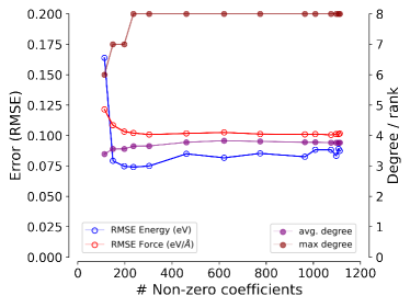
Figure 4: Effect of regularization on the full set of PA-RPI $N=4$ descriptors up to polynomial degree 24. For decreasing sparsification parameter, the root mean square training error in the energy and forces (open blue and red circles, left axis) is plotted against number of active descriptors. On the right axis, the maximum (dark red, filled circle) and average (purple, filled circle) degree is plotted. The tantalum training dataset from Ref. [​10] was used.

For some ACE models, the descriptors with high rank and degree are important. An example is provided for a metallic tantalum system; linear energy models are trained using energies and forces from the dataset in Ref. [​10] using FitSNAP with a sparsifying Bayesian compressive sensing solver. This was done using 6 single-bond descriptors along with a set of rank 2-4 ACE descriptors with $n_{max}=3$ and $l_{max}=3$. Before sparsification, the maximum degree of any $N=4$ descriptor included in the fit is 24. As shown in Fig. 4, many high-degree descriptors remain after heavy sparsification. The minimum error is achieved with a sparse model containing some high-degree descriptors. The pruning of descriptors in Fig. 4 is done using Bayesian compressive sensing, and coefficients with highest uncertainty are eliminated first. This suggests that for this small tantalum dataset, some of the highest degree descriptors correspond to an important signal in the potential that is predicted with low uncertainty compared to other descriptor coefficients. Depending on the system and the training data, high degree functions may be important. The PA-RPI procedures facilitate the use of these and other high-degree descriptors, allowing users to explore these trade-offs.

$\bm{n}$	$\bm{l}$	lex.	OCT	Num.	PA
(aaaa)	(0000)	1	1	1	1
	(1111)	2	2	1	1
	(2222)	3	3	1	1
	(3333)	4	4	2	2
	(4444)	5	5	2	2
	(5555)	6	6	2	2
	(6666)	7	7	3	3
	(7777)	8	8	3	3
(aaab)	(0000)	1	1	1	1
	(1111)	2	2	1	1
	(2222)	3	3	1	1
	(3333)	4	4	2	2
	(4444)	5	5	2	2
	(5555)	6	6	2	2
	(6666)	7	7	3	3
	(7777)	8	8	3	3
(aabb)	(0000)	1	2	1	1
	(1111)	2	4	2	2
	(2222)	3	6	3	3
	(3333)	4	8	4	4
	(4444)	5	10	5	5
	(5555)	6	12	6	6
	(6666)	7	14	7	7
	(7777)	8	16	8	8
(aabc)	(0000)	1	2	1	1
	(1111)	2	4	2	2
	(2222)	3	6	3	3
	(3333)	4	8	4	4
	(4444)	5	10	5	5
	(5555)	6	12	6	6
	(6666)	7	14	7	7
	(7777)	8	16	8	8
(abcd)	(0000)	1	3	1	1
	(1111)	2	6	3	3
	(2222)	3	9	5	5
	(3333)	4	12	7	7
	(4444)	5	15	9	9
	(5555)	6	18	11	11
	(6666)	7	21	13	13
	(7777)	8	24	15	15

(a) $\bm{l}=(\alpha\alpha\alpha\alpha)$

$\bm{n}$	$\bm{l}$	lex.	OCT	N	PA
(aaaa)	(0222)	1	1	1	1
	(1113)	1	1	1	1
	(1333)	2	2	1	1
	(2224)	2	2	1	1
	(3555)	4	4	2	2
(aaab)	(0222)	2	3	2	2
	(1113)	2	3	2	2
	(1333)	4	6	3	3
	(2224)	4	6	3	3
	(3555)	8	12	6	6
(aabb)	(0222)	2	4	2	2
	(1113)	2	4	2	2
	(1333)	4	8	4	4
	(2224)	4	8	4	4
	(3555)	8	16	8	8
(aabc)	(0222)	3	7	3	3
	(1113)	3	7	3	4
	(1333)	6	14	7	7
	(2224)	6	14	7	7
	(3555)	12	28	14	14
(abcd)	(0222)	4	12	4	4
	(1113)	4	12	4	4
	(1333)	8	24	12	12
	(2224)	8	24	12	12
	(3555)	16	48	28	28

(b) $\bm{l}=(\alpha\alpha\alpha\beta)$

Table 4: For all possibilities of equivalent $n_{i}\in\bm{n}$, we provide the $\bm{n}$ (1^st column), $\bm{l}$ (2^nd column), the number of $\bm{nlL}$ labels one obtains for a single lexicographically ordered $\bm{l}$ (3^rd column), the number of binary trees in the super set generated by step 1 of the PA-RPI procedure (4^th column), the number of independent functions as determined by semi-numerical methods (5^th column), and the number PA-RPI functions after applying step 2 of the procedure, 6^th column. This is repeated for various possible $\bm{l}$ where any 2 or more $l_{i}$ are equivalent. Variables are given in place of the actual values of $l_{i}$ for the sub-tables 4(a), 4(b).

$\bm{n}$	$\bm{l}$	lex.	OCT	N	PA
(aaaa)	(0022)	1	2	1	1
	(1122)	2	4	2	2
	(1133)	2	4	2	2
	(2233)	3	6	3	3
	(4455)	5	10	5	5
(aaab)	(0022)	2	4	2	2
	(1122)	4	8	4	4
	(1133)	4	8	4	4
	(2233)	6	12	6	6
	(4455)	10	20	10	10
(aabb)	(0022)	3	7	3	3
	(1122)	6	14	7	7
	(1133)	6	14	7	7
	(2233)	9	21	11	11
	(4455)	15	35	19	19
(aabc)	(0022)	4	10	4	4
	(1122)	8	20	10	10
	(1133)	8	20	10	10
	(2233)	12	30	16	16
	(4455)	20	50	28	28
(abcd)	(0022)	6	18	6	6
	(1122)	12	36	18	18
	(1133)	12	36	18	18
	(2233)	18	54	30	30
	(4455)	30	90	54	54

(a) $\bm{l}=(\alpha\alpha\beta\beta)$

$\bm{n}$	$\bm{l}$	lex.	OCT	N	PA
(aaaa)	(0112)	1	2	1	1
	(1223)	2	4	2	2
	(1344)	2	4	2	2
	(2455)	3	6	3	3
	(3445)	4	8	4	4
(aaab)	(0112)	3	7	3	3
	(1223)	6	14	7	7
	(1344)	6	14	7	7
	(2455)	9	21	11	11
	(3445)	12	28	15	15
(aabb)	(0112)	4	10	4	4
	(1223)	8	20	10	10
	(1344)	8	20	10	10
	(2455)	12	30	16	16
	(3445)	16	40	22	22
(aabc)	(0112)	7	19	7	7
	(1223)	14	38	19	19
	(1344)	14	38	19	19
	(2455)	21	57	31	31
	(3445)	28	76	43	43
(abcd)	(0112)	12	36	12	12
	(1223)	24	72	36	36
	(1344)	24	72	36	36
	(2455)	36	108	60	60
	(3445)	48	144	84	84

(b) $\bm{l}=(\alpha\alpha\beta\gamma)$

Table 5: For all possibilities of equivalent $n_{i}\in\bm{n}$, we provide the $\bm{n}$ (1^st column), $\bm{l}$ (2^nd column), the number of $\bm{nlL}$ labels one obtains for a single lexicographically ordered $\bm{l}$ (3^rd column), the number of binary trees in the super set generated by step 1 of the PA-RPI procedure (4^th column), the number of independent functions as determined by semi-numerical methods (5^th column), and the number PA-RPI functions after applying step 2 of the procedure, 6^th column. This is repeated for various possible $\bm{l}$ where any 2 or more $l_{i}$ are equivalent. Variables are given in place of the actual values of $l_{i}$ for the sub-tables 5(a), 5(b).

V Conclusions

The permutation-adapted RPI procedure provides a systematic way to define a complete and independent basis for ACE analytically. We relax the initial constraint that all basis labels, $\bm{nl}$, must be lexicographically ordered so that we may take advantage of the properties of the generalized Wigner symbols. After this, a basis may be defined in terms of all unique $\bm{nlL}$ indices up to automorphisms of the complete binary coupling tree and ladder relationships. The size of the PA-RPI basis is the same size as semi-numerical bases constructed in other works, and we provide some proofs to show why we and others have reported certain basis function counts for certain $\bm{nlL}$ indices. In other implementations of ACE, this reduction is done numerically. The PA-RPI methodology may help avoid numerical instabilities in some numerical methods for high-degree, high-rank descriptors.

This PA method was based on permutation properties and recursion relationships for the generalized Wigner symbols. While these properties have been explored in depth for Wigner-3j symbols, that was not the case for generalized Wigner symbols. Therefore, we have presented these properties within in detail. All of which are used to obtain new relationships that are at the heart of the PA method; the ladder relationships between functions with incremented intermediate angular momenta. The permutation symmetries provide a means to define unique permutations of basis function labels up to automorphism of the coupling tree. The combination of permutation symmetries and recursion relationships of generalized Wigner symbols allow one to derive ladder relationships between RPI basis functions. The ladder relationships are defined for a given number of duplicate $n_{i}$, $l_{i}$, and $L_{k}$, which are the radial, angular, and intermediate indices, respectively. Because the ladder relationships defined per the numbers of these duplicate indices, it is convenient to start with all unique $\bm{nlL}$ labels up to automorphism. These ladder relationships show which subsets of functions are linearly dependent, and a complete independent basis is constructed by selecting one PA function from each of these subsets. As a result, this method of constructing ACE basis functions and descriptors is based on generalizations of fundamental quantum mechanics concepts rather than singular value decomposition.

We emphasized rank 4 functions for examples throughout; they are the most simple, non-trivial cases. This method, even though it was a smaller point of discussion, was also applied to rank 5. The properties and relationships needed to apply this method to arbitrary rank have been provided though. While this method allows one to select a complete and independent ACE basis, orthogonality has not been proven. It may be a matter of deriving analytical ladder relationships for general ranks. Therefore, it would also be beneficial to explore the application of this method to higher and/or arbitrary ranks of ACE basis functions. Future work should focus on explicit proofs of orthogonality for the RPI basis using this elements of this approach. It may help assess how important these high-rank functions are in practical applications such as in interatomic potentials.

One common concern for ACE models is the large increase in the size of the ACE basis for multi-element systems and/or systems with additional degrees of freedom. Though it is not reported in depth in this work, the same principles of the PA-RPI procedure apply for atomic systems with multiple element types, or with other degrees of freedom. Significant reductions in the ACE basis indexed on additional indices, such as chemical indices $\mu_{i}$, may be achieved using the properties of the generalized Wigner symbols as well. For descriptor sets containing chemical indices, initial tests indicate that there are significant reductions in the PA-RPI basis size compared to set one needs to start with to construct semi-numerical bases.

In the most general cases, the ACE basis is restricted to be equivariant with respect to rotations. In this work, we considered primarily the case of invariance with respect to rotations. This was done to help address the immediate application of ACE bases in machine-learned interatomic potentials, but the permutation-adapted method could be generalized to select equivariant functions as well. The use of permutation automorphisms and recursion relationships for the generalized Wigner symbols is not restricted to cases where one reduces to a $L_{R}=0$ total angular momentum.

Appendix A Equivalence of generalized Wigner symbols

A.1 Wigner-3j symbols

While the traditional Clebsch-Gordan (CG) coefficients describe the addition of two angular momenta in terms of a third, the traditional Wigner-3j symbols are used in the reduction of 3 angular momenta. The traditional Clebsch-Gordan coefficients may be written as,

$$C^{l_{3},m_{3}}_{l_{1},m_{1},l_{2},m_{2}},$$ (36)

and the closely related traditional Wigner-3j symbols in symbolic and matrix form are:

$$W^{l_{3},m_{3}}_{l_{1},m_{1},l_{2},m_{2}}=\begin{pmatrix}l_{1}&l_{2}&l_{3}\\ m_{1}&m_{2}&m_{3}\end{pmatrix}.$$ (37)

Explicit algebraic forms for Eqs. (36) and (37) may be found elsewhere.Wigner (2012); Yutsis et al. (1962) For non-zero traditional Wigner-3j symbols, the triangle condition must be obeyed, $\triangle(l_{1},l_{2},l_{3})=|l_{1}-l_{2}|\leq l_{3}\leq(l_{1}+l_{2})$. Additionally, there are also conditions on the $m_{i}$. Specifically that $m_{1}+m_{2}+m_{3}=0$. From here on, the traditional Wigner-3j symbols will be used in place of the traditional Clebsch-Gordan coefficients because they have more convenient permutation symmetries. That is, the Wigner-3j symbols obey simple relationships with one another under permutations of $(l_{i},m_{i})$ tuples (columns) in matrix form. The traditional Wigner symbols obey the following relationships for odd and even permutations.

$$\begin{pmatrix}l_{1}&l_{2}&l_{3}\\ m_{1}&m_{2}&m_{3}\end{pmatrix}=(-1)^{l_{1}+l_{2}+l_{3}}\begin{pmatrix}l_{1}&l_{3}&l_{2}\\ m_{1}&m_{3}&m_{2}\end{pmatrix}=\begin{pmatrix}l_{3}&l_{1}&l_{2}\\ m_{3}&m_{1}&m_{2}\end{pmatrix}$$ (38)

Similar permutations of $(l_{i},m_{i})$ tuples in traditional CG coefficients are also equivalent, up to a phase and a scaling factor. An additional property of the traditional Wigner-3j symbols that is important when considering symmetric permutations is

$$\begin{pmatrix}l_{1}&l_{2}&0\\ m_{1}&m_{2}&0\end{pmatrix}=\delta(l_{1},l_{2})\delta(m_{1},-m_{2})\frac{(-1)^{l_{1}-m_{1}}}{\sqrt{2l_{1}+1}}$$ (39)

where $\delta(1,2)$ is the Dirac delta.Edmonds (1996) By Eq. (39), the value of non-zero Wigner-3j symbols is a phase with a scale factor when any one of the $l_{i}$ is zero.

A.2 Generalized Wigner symbols

Due to the permutation symmetries of the Wigner-3j symbols, it may be shown that the pairwise coupling scheme preserves more equivalent permutations of $l_{i}$. For the case of $N=4$ and $L_{R}=0$, the full set of equivalent permutations of leaves are shown in Fig. 5, visually and in cyclic notation. These equivalent permutations follow from three applications of Eq. (38) for each Wigner-3j comprising a rank 4 generalized symbol. In practice, we make use of this to obtain equivalent permutations of generalized Wigner symbols for arbitrary rank.

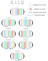
Figure 5: Illustation of equivalent permutations oof generalized Wigner symbols of rank 4. Indicies belonging to a different parent index are denoted with dotted boxes. The generalized Wigner symbols that are equivalent correspond to the permutations in the colored diagrams, with cyclic form given.

In terms of permuted tuples, the equivalent generalized Wigner symbols of rank 4 are:

$$\begin{split}\begin{pmatrix}l_{2}&l_{1}&l_{3}&l_{4}\\ m_{2}&m_{1}&m_{3}&m_{4}\end{pmatrix}\leftrightarrow\begin{pmatrix}l_{1}&l_{2}&l_{4}&l_{3}\\ m_{1}&m_{2}&m_{4}&m_{3}\end{pmatrix}\\ \leftrightarrow\begin{pmatrix}l_{1}&l_{2}&l_{3}&l_{4}\\ m_{1}&m_{2}&m_{3}&m_{4}\end{pmatrix}\leftrightarrow\begin{pmatrix}l_{2}&l_{1}&l_{4}&l_{3}\\ m_{2}&m_{1}&m_{4}&m_{3}\end{pmatrix}\\ \leftrightarrow\begin{pmatrix}l_{3}&l_{4}&l_{1}&l_{2}\\ m_{3}&m_{4}&m_{1}&m_{2}\end{pmatrix}\leftrightarrow\begin{pmatrix}l_{4}&l_{3}&l_{2}&l_{1}\\ m_{4}&m_{3}&m_{2}&m_{1}\end{pmatrix}\\ \leftrightarrow\begin{pmatrix}l_{4}&l_{3}&l_{1}&l_{2}\\ m_{4}&m_{3}&m_{1}&m_{2}\end{pmatrix}\leftrightarrow\begin{pmatrix}l_{3}&l_{4}&l_{2}&l_{1}\\ m_{3}&m_{4}&m_{2}&m_{1}\end{pmatrix}.\end{split}$$ (40)

These permutational symmetries are obeyed when the corresponding intermediate angular momenta are permuted with each coupled set of leaves, or the intermediates are equivalent $L_{1}=L_{2}$. Explicit values of such permutations were provided in Table 2. Though a set of equivalent permutations could be constructed for any arbitrary coupling scheme, it is better to choose one that belongs to the partition in Eq. (9). Otherwise the equivalent permutations may involve permutations between $l_{i}$ and $L_{k}$.

Apart from the outline provided in the main text for obtaining equivalent permutations of generalized Wigner symbols, other methods can be used to obtain them. Combining permutation symmetries for the leaves and intermediates yields a set of equivalent binary coupling trees related by a permutation operation acting on $N$ leaves and $K$ internal nodes. These permutational symmetries are known; they are elements of the automorphism group of the complete binary tree. This automorphism group is given by an iterated wreath product of the symmetric group $S_{2}$; the wreath product is performed $h$ times where $h$ is the height of the binary tree, given from Eq. (11).Brunner and Sidki (1997)

$$H_{1}=S_{2}$$ (41a)

$$H_{2}=S_{2}\wr S_{2}$$ (41b)

$$H_{h}=H_{h-1}\wr S_{2}$$ (41c)

The group of automorphisms generated in Eq. (41a) may be defined for any arbitrary binary tree of height $h$, by iterating the wreath product $h$ times, Eq. (41c). However, only a subset of $H_{h}$ is needed when considering angular momentum coupling trees. Some elements of $H_{h}$ include permutations of the root node, $L_{R}$ in our case, with internal nodes $L_{k}$. This could result in couplings that are not rotationally invariant. To address this, aone could select a subset of $H_{h}$ is selected that preserves the level of the node values (e.g. $l_{i}$ cannot be permuted with $L_{k}$). Additionally, this set of permutation automorphisms may change with the number of duplicate leaf indices, $(l_{i},m_{i})$, and/or the number of duplicate intermediates $L_{k}$. As a result, a more specific set of $H_{h}$ that accounts for duplicate may be collected into $G_{N}$. It is constructed in general by starting with $H_{h}$ and removing elements that permute between levels of the coupling tree. This set of automorphisms can be generated for arbitrary coupling rank, $N$ with height given by Eq. (11). This is one of the convenient features of the pairwise coupling scheme used for generalized Wigner symbols in this work; the coupling tree for the generalized Wigner symbols has the same structure as the complete binary tree.

A.3 Explicit proof for rank 4 equivalences

The rank 4 generalized Wigner symbols with a $\sigma_{c}=(1,2)(3,4)$ coupling scheme may be explicitly written, from Eq. 10.3 of Ref. [​3] as,

$$\begin{split}\begin{pmatrix}l_{1}&l_{2}&l_{3}&l_{4}\\ m_{1}&m_{2}&m_{3}&m_{4}\end{pmatrix}^{(1,2)(3,4)}_{L_{1},L_{2},L_{R}}=\sum_{M_{1},M_{2}}(-1)^{L_{1}-M_{1}}(-1)^{L_{2}-M_{2}}\begin{pmatrix}l_{1}&l_{2}&L_{1}\\ m_{1}&m_{2}&-M_{1}\end{pmatrix}\\ \begin{pmatrix}l_{3}&l_{4}&L_{2}\\ m_{3}&m_{4}&-M_{2}\end{pmatrix}\begin{pmatrix}L_{1}&L_{2}&L_{R}\\ M_{1}&M_{2}&M_{R}\end{pmatrix}\end{split}$$ (42)

Here, the case of $L_{R}=0$ is considered, for which the generalized symbols are non-zero only when $M_{R}=0$, $L_{1}=L_{2}=L$, $M_{1}=-M_{2}=M$, $m_{1}+m_{2}=M$, and $m_{3}+m_{4}=-M$. As a result of these restrictions, only a single non-zero term remains

$$\begin{split}\begin{pmatrix}l_{1}&l_{2}&l_{3}&l_{4}\\ m_{1}&m_{2}&m_{3}&m_{4}\end{pmatrix}^{(1,2)(3,4)}_{L,L,L_{R}=0}=\frac{1}{\sqrt{2L+1}}(-1)^{L-M}\begin{pmatrix}l_{1}&l_{2}&L\\ m_{1}&m_{2}&-M\end{pmatrix}\begin{pmatrix}l_{3}&l_{4}&L\\ m_{3}&m_{4}&M\end{pmatrix}\end{split}$$ (43)

where we have used Eq. (39) to eliminate the third Wigner-3j symbol. By Eq. (38), the values of the two traditional Wigner coefficients are unaffected by permutation of the columns, up to a phase change. Hence the full expression is invariant up to a phase change under any permutation $\sigma\in G_{N}$. These equivalent permutations may be categorized a few ways. The first: permutation between pairs of $l_{i}$ that are coupled (e.g. $l_{1}$ and $l_{2}$ may be permuted under the parent, $L_{1}$, 2). The second: a permutation of coupled branches (e.g. permuting children of $L_{R}$ for rank 4 trees: $L_{1}$ and $L_{2}$ may be permuted, then all corresponding children of $L_{1}$ and $L_{2}$ such that the order in the sub-trees $[l_{1},l_{2}]$ and $[l_{3},l_{4}]$ are preserved). The third: some combination of the first and second kinds of equivalent permutations (cf. Eq. (40) and Fig. 5). For the case $\sigma_{\circ}(\bm{l})=(1234)(22)$ and $\bm{m}=(1,-2,-3,4)$ shown in Table  2, we can use the above expression to obtain

$$\begin{split}\begin{pmatrix}1&2&3&4\\ 1&-2&-3&4\end{pmatrix}^{(1,2)(3,4)}_{2,2,L_{R}=0}=\frac{-1}{\sqrt{5}}\begin{pmatrix}1&2&2\\ 1&-2&1\end{pmatrix}\begin{pmatrix}3&4&2\\ -3&4&-1\end{pmatrix}=\frac{1}{\sqrt{1125}}\end{split}$$ (44)

Conversely, for permutations across the intermediate coupling such as $(1,3)\notin G_{N}$, we get:

$$\begin{split}\begin{pmatrix}l_{3}&l_{2}&l_{1}&l_{4}\\ m_{3}&m_{2}&m_{1}&m_{4}\end{pmatrix}^{(1,2)(3,4)}_{L,L,L_{R}=0}=\frac{1}{\sqrt{2L+1}}(-1)^{L-M}\begin{pmatrix}l_{3}&l_{2}&L\\ m_{3}&m_{2}&-M\end{pmatrix}\begin{pmatrix}l_{1}&l_{4}&L\\ m_{1}&m_{4}&M\end{pmatrix}\end{split}$$ (45)

which is not equivalent to the original rank 4 generalized Wigner symbol. Note that symmetry breaking occurs with certain permutations that span indices in distinct symmetric pairs. Similar proofs of permutational symmetries are straightforward to construct for generalized Wigner symbols of arbitrary rank. This is why it is often just mentioned in other work.Yutsis et al. (1962) In the main text, the group of all permutation automorphisms for the coupling trees are obtained from Eq. (41c).

Appendix B Ladder relationships

B.1 Recursion relationships for Wigner symbols

In this section we provide a detailed and thorough background for the properties of the Wigner symbols when quantum numbers are raised or lowered. From p. 224 of Rose’s ”Elementary Theory of Angular Momentum” (1957), there are raising/lowering (a.k.a ladder) operations that lead to recursion relationships between Clebsch-Gordan coefficients of increasing/decreasing principal quantum numbers.

$$\begin{split}\bigg{[}m_{1}-m_{3}\bigg{(}\frac{l_{1}(l_{1}+1)-l_{2}(l_{2}+1)+l_{3}(l_{3}+1)}{2l_{3}(l_{3}+1)}\bigg{)}\bigg{]}\begin{bmatrix}l_{1}&l_{2}&l_{3}\\ m_{1}&m_{2}&m_{3}\end{bmatrix}=\\ \bigg{[}\frac{\big{(}(l_{3})^{2}-(m_{3})^{2}\big{)}(l_{2}+l_{3}-l_{1})(l_{1}+l_{3}-l_{2})(l_{1}+l_{2}-l_{3}+1)(l_{1}+l_{2}+l_{3}+1)}{4(l_{3})^{2}(2l_{3}-1)(2l_{3}+1)}\bigg{]}^{1/2}\begin{bmatrix}l_{1}&l_{2}&l_{3}-1\\ m_{1}&m_{2}&m_{3}\end{bmatrix}+\\ \bigg{[}\frac{((l_{3}+1)^{2}-(m_{3})^{2})(1+l_{2}+l_{3}-l_{1})(1+l_{1}+l_{3}-l_{2})(l_{1}+l_{2}-l_{3})(l_{1}+l_{2}+l_{3}+2)}{4(l_{3}+1)^{2}(2l_{3}+1)(2l_{3}+3)}\bigg{]}^{1/2}\begin{bmatrix}l_{1}&l_{2}&l_{3}+1\\ m_{1}&m_{2}&m_{3}\end{bmatrix}\end{split}$$ (46)

and in the form of Wigner-3j symbols:

$$\begin{split}&\bigg{[}m_{1}-m_{3}\bigg{(}\frac{l_{1}(l_{1}+1)-l_{2}(l_{2}+1)+l_{3}(l_{3}+1)}{2l_{3}(l_{3}+1)}\bigg{)}\bigg{]}\begin{pmatrix}l_{1}&l_{2}&l_{3}\\ m_{1}&m_{2}&-m_{3}\end{pmatrix}(\sqrt{2l_{3}+1})=\\ &\bigg{[}\frac{\big{(}(l_{3})^{2}-(m_{3})^{2}\big{)}(l_{2}+l_{3}-l_{1})(l_{1}+l_{3}-l_{2})(l_{1}+l_{2}-l_{3}+1)(l_{1}+l_{2}+l_{3}+1)}{4(l_{3})^{2}(2l_{3}-1)(2l_{3}+1)}\bigg{]}^{1/2}\begin{pmatrix}l_{1}&l_{2}&l_{3}-1\\ m_{1}&m_{2}&-m_{3}\end{pmatrix}(\sqrt{2l_{3}})+\\ &\bigg{[}\frac{((l_{3}+1)^{2}-(m_{3})^{2})(1+l_{2}+l_{3}-l_{1})(1+l_{1}+l_{3}-l_{2})(l_{1}+l_{2}-l_{3})(l_{1}+l_{2}+l_{3}+2)}{4(l_{3}+1)^{2}(2l_{3}+1)(2l_{3}+3)}\bigg{]}^{1/2}\begin{pmatrix}l_{1}&l_{2}&l_{3}+1\\ m_{1}&m_{2}&-m_{3}\end{pmatrix}(\sqrt{2(l_{3}+1)})\end{split}$$ (47)

For the purposes of comparing different intermediate angular momenta, it will often be sufficient to express Eq. (47) as

$$\begin{pmatrix}l_{1}&l_{2}&l_{3}\\ m_{1}&m_{2}&-m_{3}\end{pmatrix}=A_{-}(l_{1},l_{2},l_{3},m_{1},m_{3})\begin{pmatrix}l_{1}&l_{2}&l_{3}-1\\ m_{1}&m_{2}&-m_{3}\end{pmatrix}+A_{+}(l_{1},l_{2},l_{3},m_{1},m_{3})\begin{pmatrix}l_{1}&l_{2}&l_{3}+1\\ m_{1}&m_{2}&-m_{3}\end{pmatrix},$$ (48)

because only the principle quantum number in the third column changes. The most general notation suggests that coupling coefficients incremented by an integer value are related to others by factors $A_{+}$ and $A_{-}$. These factors in Eq. (48) depend on all quantum numbers in the coupling coefficient (all $l_{i}$ and all $m_{i}$). However, this can be simplified when one takes triangle conditions into account as well as the fact that $m_{3}=m_{1}+m_{2}$.

Note that triangle conditions state: $|l_{1}-l_{2}|\leq l_{3}\leq l_{1}+l_{3}$, therefore $\min(l_{3})=|l_{1}-l_{2}|$. From here on, this minimum value of $l_{3}$ will be denoted as $\mathcal{L}$. It depends only on $l_{1}$ and $l_{2}$. Incrementing the third principle quantum number from this minimum value gives,

$$\begin{split}&\begin{pmatrix}l_{1}&l_{2}&\mathcal{L}+1\\ m_{1}&m_{2}&-m_{3}\end{pmatrix}=A_{+}(l_{1},l_{2},m_{1},m_{2},0)\cdot{}\begin{pmatrix}l_{1}&l_{2}&\mathcal{L}+1\\ m_{1}&m_{2}&-m_{3}\end{pmatrix}\end{split}$$ (49)

where the first term is zero due to triangle conditions. For the dependence of the $A_{+}$ and $A_{-}$ coefficients, they now only depend on the first two angular momentum quantum numbers and an increment $k=0$, that $L$ is incremented by. The result of Eq. (49) shows that the Wigner symbol with $l_{3}=\mathcal{L}$ is linearly related to that for $\mathcal{L}+1$.

To find relationships with other values of $l_{3}$, this relationship will be applied multiple times from the minimum, $\mathcal{L}$. For the next principal quantum number:

$$\begin{split}&\begin{pmatrix}l_{1}&l_{2}&\mathcal{L}+1\\ m_{1}&m_{2}&-m_{3}\end{pmatrix}=A_{-}^{\prime}(l_{1},l_{2},m_{1},m_{2},1)A_{+}(l_{1},l_{2},m_{1},m_{3},0)\cdot\begin{pmatrix}l_{1}&l_{2}&\mathcal{L}\\ m_{1}&m_{2}&-m_{3}\end{pmatrix}\\ &+A_{+}^{\prime}(l_{1},l_{2},m_{1},m_{2},1)\cdot\begin{pmatrix}l_{1}&l_{2}&\mathcal{L}+2\\ m_{1}&m_{2}&-m_{3}\end{pmatrix}.\end{split}$$ (50)

Here, the increment increases by one, $k=1$, and is given as the last term in the parenthesis of the $A_{\pm}^{\prime}$. Substituting the relationship from Eq. (49) yields:

$$\begin{split}&\begin{pmatrix}l_{1}&l_{2}&\mathcal{L}+1\\ m_{1}&m_{2}&-m_{3}\end{pmatrix}=A_{-}^{\prime}(l_{1},l_{2},m_{1},m_{2},1)\bigg{(}A_{+}(l_{1},l_{2},m_{1},m_{3},0)\cdot\begin{pmatrix}l_{1}&l_{2}&\mathcal{L}+1\\ m_{1}&m_{2}&-m_{3}\end{pmatrix}\bigg{)}\\ &+A_{+}^{\prime}(l_{1},l_{2},m_{1},m_{2},1)\cdot\begin{pmatrix}l_{1}&l_{2}&\mathcal{L}+2\\ m_{1}&m_{2}&-m_{3}\end{pmatrix}\end{split}$$ (51)

As a result, the Wigner symbol for $\mathcal{L}+1$ is linearly related to that of $\mathcal{L}+2$. The expression in Eq. (51) simplifies further upon substitution of Eq. (49) to

$$\begin{split}&\begin{pmatrix}l_{1}&l_{2}&\mathcal{L}\\ m_{1}&m_{2}&-m_{3}\end{pmatrix}=\frac{A_{+}(l_{1},l_{2},m_{1},m_{2},0)A_{+}^{\prime}(l_{1},l_{2},m_{1},m_{2},1)}{(1-A_{-}^{\prime}(l_{1},l_{2},m_{1},m_{2},1)A_{+}(l_{1},l_{2},m_{1},m_{2},0))}\cdot\begin{pmatrix}l_{1}&l_{2}&\mathcal{L}+2\\ m_{1}&m_{2}&-m_{3}\end{pmatrix}\\ &=f_{1}(l_{1},l_{2},m_{1},m_{2},k_{1}=1)\cdot\begin{pmatrix}l_{1}&l_{2}&\mathcal{L}+2\\ m_{1}&m_{2}&-m_{3}\end{pmatrix}\end{split}$$ (52)

This may be iterated for all remaining principal quantum numbers up to the maximum value of $l_{1}+l_{2}$. It should also be noted that all terms in the linear factor may be written explicitly in terms of $\mathcal{L},l_{1},l_{2}$, and $m_{1},m_{2}$. As a result, with $l_{1}$, $l_{2}$, $m_{1}$, and $m_{2}$, held constant, all possible values of the principal quantum number yield linearly dependent Wigner-3j symbols. All Wigner-3j symbols related by this operation may be expressed in terms of the Wigner-3j symbol for $\mathcal{L}$ multiplied by some factor. By simple relationships between CG coefficients and Wigner-3j symbols, these linear dependencies extend to Clebsch-Gordan coefficients.

A simplified expression will be used for arbitrary increments $k$ from the lowest allowed value, $\bm{L}$.

$$\begin{pmatrix}l_{1}&l_{2}&\mathcal{L}_{1}\\ m_{1}&m_{2}&M_{1}\end{pmatrix}=f_{1}(l_{1},l_{2},m_{1},m_{2},k_{1})\begin{pmatrix}l_{1}&l_{2}&\mathcal{L}_{1}+k_{1}\\ m_{1}&m_{2}&M_{1}\end{pmatrix}$$ (53)

which follows from the recursion relationships described above. An index on the third principal quantum number will be necessary when considering generalized coupling coefficients. In addition, it is important to note that the projection, $M_{1}$, is constrained by the values $m_{1}$ and $m_{2}$ as well as the final projection quantum number $M_{R}$.

Additional raising/lowering operations exist for incremented projection quantum numbers in the Wigner-3j Wigner symbols. The first set is:

$$\begin{split}&\begin{pmatrix}l_{1}&l_{2}&l_{3}\\ m_{1}&m_{2}&m_{3}\pm 1\end{pmatrix}=\\ &\mathcal{J}\bigg{[}\frac{l_{1}(l_{1}+1)-m_{1}(m_{1}\mp 1)}{l_{3}(l_{3}+1)-m_{3}(m_{3}\pm 1)}\bigg{]}^{1/2}\begin{pmatrix}l_{1}&l_{2}&l_{3}\\ m_{1}\mp 1&m_{2}&m_{3}\end{pmatrix}+\mathcal{J}\bigg{[}\frac{l_{2}(l_{2}+1)-m_{2}(m_{2}\mp 1)}{l_{3}(l_{3}+1)-m_{3}(m_{3}\pm 1)}\bigg{]}^{1/2}\begin{pmatrix}l_{1}&l_{2}&l_{3}\\ m_{1}&m_{2}\mp 1&m_{3}\end{pmatrix}\end{split}.$$ (54)

To compare different intermediate angular momenta in generalized Wigner symbols, it will be sufficient to express the prefactors as constants with respect to $l_{3}$. This takes the form:

$$\begin{split}&\begin{pmatrix}l_{1}&l_{2}&l_{3}\\ m_{1}&m_{2}&m_{3}\pm 1\end{pmatrix}=G(l_{1},l_{3},m_{1},m_{3})\begin{pmatrix}l_{1}&l_{2}&l_{3}\\ m_{1}\mp 1&m_{2}&m_{3}\end{pmatrix}+H(l_{2},l_{3},m_{2},m_{3})\begin{pmatrix}l_{1}&l_{2}&l_{3}\\ m_{1}&m_{2}\mp 1&m_{3}\end{pmatrix}\end{split},$$ (55)

where $G$ and $H$ are factors that depend on both angular momentum quantum numbers and projection quantum numbers, and $\mathcal{J}=\sqrt{2l_{3}+1}$. Similar to the recursion relationships derived for the angular momentum quantum numbers, there are ways to reduce the number of variables that $G$ and $H$ depend on.

The final raising/lowering operation discussed for traditional couplings are those in the projection quantum numbers for fixed $m_{3}$. One may derive, as in Rose 1957, that:

$$\begin{split}&\begin{pmatrix}l_{1}&l_{2}&l_{3}\\ m_{1}&m_{2}&m_{3}\end{pmatrix}=P_{+}\begin{pmatrix}l_{1}&l_{2}&l_{3}\\ m_{1}-1&m_{2}+1&m_{3}\end{pmatrix}+P_{-}\begin{pmatrix}l_{1}&l_{2}&l_{3}\\ m_{1}+1&m_{2}-1&m_{3}\end{pmatrix}\end{split},$$ (56)

where $P_{\pm}$ is given by,

$$\mathcal{J}\;\frac{\sqrt{(l_{1}\pm m_{1})(l_{2}\mp m_{2})(l_{1}\mp m_{1}+1)(l_{2}\pm m_{2}+1)}}{l_{3}(l_{3}+1)-l_{1}(l_{1}+1)-l_{2}(l_{2}+1)-2m_{1}m_{2}}.$$ (57)

These are the key recursion relationships for the traditional Wigner-3j symbols. The generalized Wigner symbols used to construct ACE invariants are comprised of contractions of multiple traditional Wigner-3j symbols. The recursion relationships for generalized Wigner symbols have not yet been derived, but one may obtain them by applying the recursion relationships for each traditional Wigner-3j symbol in the generalized Wigner symbol.

B.2 Recursion relationships between generalized Wigner symbols

These recursion relationships will now be derived for the rank 4 generalized Wigner symbols. Note that the rank 4 generalized Wigner symbol with the lowest possible intermediates is given as,

$$\begin{split}&\begin{pmatrix}l_{1}&l_{2}&l_{3}&l_{4}\\ m_{1}&m_{2}&m_{3}&m_{4}\end{pmatrix}\big{(}\mathcal{L}_{1},\mathcal{L}_{2}\big{)}\\ &\sum_{M_{1},M_{2}}(-1)^{(\mathcal{L}_{1}-M_{1}+\mathcal{L}_{2}-M_{2})}\begin{pmatrix}l_{1}&l_{2}&\mathcal{L}_{1}\\ m_{1}&m_{2}&-(m_{1}+m_{2})\end{pmatrix}\begin{pmatrix}l_{3}&l_{4}&\mathcal{L}_{2}\\ m_{3}&m_{4}&-(m_{3}+m_{4})\end{pmatrix}\\ &\begin{pmatrix}\mathcal{L}_{1}&\mathcal{L}_{2}&L_{R}\\ (m_{1}+m_{2})&(m_{3}+m_{4})&-M_{R}\end{pmatrix}\end{split}$$ (58)

The phase, $(-1)^{(\mathcal{L}_{1}-M_{1}+\mathcal{L}_{2}-M_{2})}$, may be omitted or represented as $\phi(\bm{l},\bm{m},\bm{k})$ if the intermediate angular momenta are incremented by $\bm{k}=(k_{1},k_{2},\cdots k_{N})$. If written as, $\phi(\bm{l},\bm{m}$ the phase does not explicitly depend on the increments. The form of this phase is derived for arbitrary rank in Yutsis.Yutsis et al. (1962) It is sufficient here to know that in general, it depends on all intermediate angular momentum quantum numbers and all intermediate projection quantum numbers. For all $k$ allowed by triangle conditions, one obtains:

$$\begin{split}&\begin{pmatrix}l_{1}&l_{2}&l_{3}&l_{4}\\ m_{1}&m_{2}&m_{3}&m_{4}\end{pmatrix}\big{(}\mathcal{L}_{1}+k_{1},\mathcal{L}_{2}+k_{2}\big{)}=\\ &\phi(\bm{l},\bm{m},\bm{k})f_{12}(l_{1},l_{2},m_{1},m_{2},k_{1})\begin{pmatrix}l_{1}&l_{2}&\mathcal{L}_{1}\\ m_{1}&m_{2}&-(m_{1}+m_{2})\end{pmatrix}f_{34}(l_{3},l_{4},m_{3},m_{4},k_{2})\begin{pmatrix}l_{3}&l_{4}&\mathcal{L}_{2}\\ m_{3}&m_{4}&-(m_{3}+m_{4})\end{pmatrix}\\ &\begin{pmatrix}\mathcal{L}_{1}+k_{1}&\mathcal{L}_{2}+k_{2}&L_{R}\\ (m_{1}+m_{2})&(m_{3}+m_{4})&-M_{R}\end{pmatrix}\end{split}$$ (59)

Where the recursion relationship in Eq. (53) has been substituted for the first two constituent Wigner-3j symbols, and the sum over $M_{1},M_{2}$ is simplified by replacing $M_{1}$ and $M_{2}$ with $(m_{1}+m_{2})$ and $(m_{3}+m_{4})$, respectively. Other projection quantum numbers would result in zero-valued summands. Here, each traditional Wigner-3j symbol that couples $l_{i}$ has a factor $f_{12}$ and $f_{34}$ for increments of $L_{1}$ and $L_{2}$. The final factor in Eq. (59) will also obey ladder relationships with its principal quantum numbers. Applying the recursion relationship for the index of $\mathcal{L}_{1}$ and again for the index of $L_{2}$ gives:

$$\begin{split}&\begin{pmatrix}\mathcal{L}_{1}+k_{1}&\mathcal{L}_{2}+k_{2}&L_{R}\\ (m_{1}+m_{2})&(m_{3}+m_{4})&-M_{R}\end{pmatrix}=\\ &f_{12}^{\prime}(l_{1},l_{2},m_{1},m_{2},k_{1},k_{2})f_{34}^{\prime}(l_{3},l_{4},m_{3},m_{4},k_{2})\begin{pmatrix}\mathcal{L}_{1}&\mathcal{L}_{2}&L_{R}\\ (m_{1}+m_{2})&(m_{3}+m_{4})&-M_{R}\end{pmatrix}\end{split},$$ (60)

where the factors $f_{12}^{\prime}$ and $f_{34}^{\prime}$ depend on the order in which the recursion relationships are applied. recursion relationships were applied for $L_{1}$ first then $L_{2}$ second in Eq. (60), but this is arbitrary due to the permutational symmetries of traditional Wigner-3j symbols. Regardless, a linear relationship may be obtained for the third Wigner symbol. Combining the recursion relationships from Eq. (53) for all three traditional Wigner-3j symbols that comprise the generalized symbol gives the following.

$$\begin{split}&F(\bm{l},\bm{m},k_{1},k_{2})F^{\prime}(\bm{l},\bm{m},k_{1},k_{2})\begin{pmatrix}l_{1}&l_{2}&l_{3}&l_{4}\\ m_{1}&m_{2}&m_{3}&m_{4}\end{pmatrix}\big{(}\mathcal{L}_{1},\mathcal{L}_{2}\big{)}=\begin{pmatrix}l_{1}&l_{2}&l_{3}&l_{4}\\ m_{1}&m_{2}&m_{3}&m_{4}\end{pmatrix}\big{(}\mathcal{L}_{1}+k_{1},\mathcal{L}_{2}+k_{2}\big{)}\\ &\begin{pmatrix}l_{1}&l_{2}&l_{3}&l_{4}\\ m_{1}&m_{2}&m_{3}&m_{4}\end{pmatrix}\big{(}\mathcal{L}_{1},\mathcal{L}_{2}\big{)}=\mathcal{A}(\bm{l},\bm{m},k_{1},k_{2})\begin{pmatrix}l_{1}&l_{2}&l_{3}&l_{4}\\ m_{1}&m_{2}&m_{3}&m_{4}\end{pmatrix}\big{(}\mathcal{L}_{1}+k_{1},\mathcal{L}_{2}+k_{2}\big{)}\end{split}$$ (61)

where the substitutions of $F(\bm{l},\bm{m},k_{1},k_{2})=f_{12}(l_{1},l_{2},m_{1},m_{2},k_{1})f_{34}(l_{3},l_{4},m_{3},m_{4},k_{2})$ and $F^{\prime}(\bm{l},\bm{m},k_{1},k_{2})=f_{12}^{\prime}(l_{1},l_{2},m_{1},m_{2},k_{1},k_{2})f_{34}^{\prime}(l_{3},l_{4},m_{3},m_{4},k_{2})$ have been made. Despite the complicated form of the prefactor, $\mathcal{A}(\bm{l},\bm{m},k_{1},k_{2})$, Eq. (61) shows what the exact linear relationship between rank 4 Wigner symbols with different intermediates is. All terms in $\mathcal{A}_{+,+}$ may be written in terms of $l_{1},l_{2},l_{3},l_{4}$ and $m_{1},m_{2},m_{3},m_{4}$. This is derived here for the pairwise coupling scheme, but it is easily extended to others.

The relationships between generalized Wigner symbols with arbitrary intermediates may be derived by applying the raising/lowering operations for each constituent traditional Wigner-3j symbol, as was done to obtain Eq. (61). In general one may write:

$$\begin{split}&\begin{pmatrix}l_{1}&l_{2}&l_{3}&l_{4}\\ m_{1}&m_{2}&m_{3}&m_{4}\end{pmatrix}\big{(}L_{1},L_{2}\big{)}=\\ &A_{-,-}(\bm{l},\bm{m})\begin{pmatrix}l_{1}&l_{2}&l_{3}&l_{4}\\ m_{1}&m_{2}&m_{3}&m_{4}\end{pmatrix}\big{(}L_{1}-1,L_{2}-1\big{)}+A_{-,+}(\bm{l},\bm{m})\begin{pmatrix}l_{1}&l_{2}&l_{3}&l_{4}\\ m_{1}&m_{2}&m_{3}&m_{4}\end{pmatrix}\big{(}L_{1}-1,L_{2}+1\big{)}\\ &+A_{+,-}(\bm{l},\bm{m})\begin{pmatrix}l_{1}&l_{2}&l_{3}&l_{4}\\ m_{1}&m_{2}&m_{3}&m_{4}\end{pmatrix}\big{(}L_{1}+1,L_{2}-1\big{)}+A_{+,+}(\bm{l},\bm{m})\begin{pmatrix}l_{1}&l_{2}&l_{3}&l_{4}\\ m_{1}&m_{2}&m_{3}&m_{4}\end{pmatrix}\big{(}L_{1}+1,L_{2}+1\big{)}\end{split}$$ (62)

which, for $L_{R}=0$ reduces to:

$$\begin{split}&\begin{pmatrix}l_{1}&l_{2}&l_{3}&l_{4}\\ m_{1}&m_{2}&m_{3}&m_{4}\end{pmatrix}\big{(}L_{1},L_{2}\big{)}=\\ &A_{-,-}(\bm{l},\bm{m})\begin{pmatrix}l_{1}&l_{2}&l_{3}&l_{4}\\ m_{1}&m_{2}&m_{3}&m_{4}\end{pmatrix}\big{(}L_{1}-1,L_{2}-1\big{)}+A_{+,+}(\bm{l},\bm{m})\begin{pmatrix}l_{1}&l_{2}&l_{3}&l_{4}\\ m_{1}&m_{2}&m_{3}&m_{4}\end{pmatrix}\big{(}L_{1}+1,L_{2}+1\big{)}\end{split}$$ (63)

In Eq. (63) the $A_{\pm,\pm}(\bm{l},\bm{m})$ factors, similar to those defined in terms of $\mathcal{L}_{1},\mathcal{L}_{2}$ are products of factors from raising/lowering traditional Wigner-3j symbols.

In addition to recursion relationships between intermediates angular momentum quantum numbers with different values, one can also derive raising and lowering relationships between intermediate projection quantum numbers. The relationships between different projection quantum numbers will also be demonstrated for rank 4, but are easily generalized. In these recursion relationships all angular momentum quantum numbers will be fixed, including the intermediates. For some intermediate projections $M_{1}$ and $M_{2}$, one may raise and/or lower the projection quantum numbers according to,

$$\begin{split}&\begin{pmatrix}l_{1}&l_{2}&l_{3}&l_{4}\\ m_{1}&m_{2}&m_{3}&m_{4}\end{pmatrix}\big{(}M_{1}\pm 1,M_{2}\mp 1,M_{R}\big{)}=\\ &\phi(\bm{l},\bm{m})\bigg{[}G_{1}(l_{1},L_{1},m_{1},M_{1})\begin{pmatrix}l_{1}&l_{2}&L_{1}\\ m_{1}\mp 1&m_{2}&M_{1}\end{pmatrix}+H_{1}(l_{2},L_{1},m_{2},M_{1})\begin{pmatrix}l_{1}&l_{2}&L_{1}\\ m_{1}&m_{2}\mp 1&M_{1}\end{pmatrix}\bigg{]}\\ &\bigg{[}G_{2}(l_{3},L_{2},m_{3},M_{2})\begin{pmatrix}l_{3}&l_{4}&L_{2}\\ m_{3}\pm 1&m_{4}&M_{2}\end{pmatrix}+H_{2}(l_{4},L_{2},m_{4},M_{2})\begin{pmatrix}l_{3}&l_{4}&L_{1}\\ m_{3}&m_{4}\pm 1&M_{2}\end{pmatrix}\bigg{]}\\ &\bigg{[}P_{\pm}\begin{pmatrix}L_{1}&L_{2}&L_{R}\\ M_{1}&M_{2}&M_{R}\end{pmatrix}\bigg{]},\end{split}$$ (64)

where the phase $\phi(\bm{l},\bm{m})$ depends on $m_{i}$ that have been incremented. Notice that in Eq. (64), the $M_{k}$ is incremented such that the root projection quantum number $M_{R}$ is conserved. The third bracketed term in this equation only has one value rather than the two from Eq. (56); one of the terms will always be zero due to the valid domain of $m_{i}$ and $M_{k}$. One particularly convenient result of this relationship is that a generalized coupling coefficient with a set of intermediate projections $\bm{M}$ may be written in terms of a sum of generalized coupling coefficients with a different set of intermediate projections, $\bm{M}^{\prime}$. Explicitly after distributing in Eq. (64), one obtains:

$$\begin{split}&\begin{pmatrix}l_{1}&l_{2}&l_{3}&l_{4}\\ m_{1}&m_{2}&m_{3}&m_{4}\end{pmatrix}\big{(}M_{1}\pm 1,M_{2}\mp 1,M_{R}\big{)}=\\ &\phi(\bm{l},\bm{m})\bigg{[}G_{1}(l_{1},L_{1},m_{1},M_{1})G_{2}(l_{3},L_{2},m_{3},M_{2})P_{+}\begin{pmatrix}l_{1}&l_{2}&l_{3}&l_{4}\\ m_{1}\mp 1&m_{2}&m_{3}\pm 1&m_{4}\end{pmatrix}\big{(}M_{1},M_{2},M_{R}\big{)}\\ &+G_{1}(l_{1},L_{1},m_{1},M_{1})H_{2}(l_{4},L_{2},m_{4},M_{2})P_{+}\begin{pmatrix}l_{1}&l_{2}&l_{3}&l_{4}\\ m_{1}\mp 1&m_{2}&m_{3}&m_{4}\pm 1\end{pmatrix}\big{(}M_{1},M_{2},M_{R}\big{)}\\ &+H_{1}(l_{2},L_{1},m_{2},M_{1})G_{2}(l_{3},L_{2},m_{3},M_{2})P_{-}\begin{pmatrix}l_{1}&l_{2}&l_{3}&l_{4}\\ m_{1}&m_{2}\mp 1&m_{3}\pm 1&m_{4}\end{pmatrix}\big{(}M_{1},M_{2},M_{R}\big{)}\\ &+H_{1}(l_{2},L_{1},m_{2},M_{1})H_{2}(l_{4},L_{2},m_{4},M_{2})P_{-}\begin{pmatrix}l_{1}&l_{2}&l_{3}&l_{4}\\ m_{1}&m_{2}\mp 1&m_{3}&m_{4}\pm 1\end{pmatrix}\big{(}M_{1},M_{2},M_{R}\big{)}\bigg{]},\end{split}$$ (65)

which again holds true for fixed $\bm{lL}$ in the pairwise coupling scheme. In general, one may write the expression above in terms of a sum over intermediate projection quantum numbers:

$$\begin{split}&\begin{pmatrix}l_{1}&l_{2}&l_{3}&l_{4}\\ m_{1}&m_{2}&m_{3}&m_{4}\end{pmatrix}\big{(}\{M_{1}\pm 1,M_{2}\mp 1\},M_{R}\big{)}=\sum_{\bm{\mathcal{M}}}c_{\bm{\mathcal{M}}}\begin{pmatrix}l_{1}&l_{2}&l_{3}&l_{4}\\ m_{1}^{\prime}&m_{2}^{\prime}&m_{3}^{\prime}&m_{4}^{\prime}\end{pmatrix}\big{(}\{M_{1},M_{2}\},M_{R}\big{)}\end{split}$$ (66)

where $\bm{\mathcal{M}}=\{M_{1},M_{2}\}$ are the intermediate projection quantum numbers with $m_{i}$ obeying the recursion relationship in Eq. (65) (e.g. $M_{1}=m_{1}\mp 1+m_{2})$) and the $c_{\bm{\mathcal{M}}}$ are the coefficients containing products of $H_{k}$, $G_{k}$, and $P_{\mp}$ from Eqs. (55) and (56), respectively. In principle the coefficients in Eq. (66) can be written in terms of minimum/maximum values of $M_{i}$ allowed by their corresponding intermediates $\mathcal{L}_{i}$.

B.3 Recursion relationships for generalized Wigner symbols with arbitrary rank

These recursion relationships can also be used to show linear relationships between generalized Wigner symbols of higher rank. In the pairwise coupling scheme, the linear relationships between different intermediates may be given for Wigner symbols of arbitrary rank.

$$\begin{split}&\begin{pmatrix}l_{1}&l_{2}&l_{3}&\cdots&l_{N}\\ m_{1}&m_{2}&m_{3}&\cdots&m_{N}\end{pmatrix}\big{(}\mathcal{L}_{1}+k_{1},\mathcal{L}_{2}+k_{2},\cdots\mathcal{L}_{(N-2)}+k_{(N-2)}\big{)}=\\ &\phi(\bm{l},\bm{m},\bm{k})f_{12}(l_{1},l_{2},m_{1},m_{2},k_{1})\begin{pmatrix}l_{1}&l_{2}&\mathcal{L}_{1}\\ m_{1}&m_{2}&-(m_{1}+m_{2})\end{pmatrix}f_{34}(l_{3},l_{4},m_{3},m_{4},k_{2})\begin{pmatrix}l_{3}&l_{4}&\mathcal{L}_{2}\\ m_{3}&m_{4}&-(m_{3}+m_{4})\end{pmatrix}\\ &\cdots f_{(N-1,N)}(l_{(N-1)},l_{N},m_{(N-1)},m_{N})\begin{pmatrix}l_{(N-1)}&l_{N}&\mathcal{L}_{N/2}\\ m_{(N-1)}&m_{N}&-(m_{(N-1)}+m_{N})\end{pmatrix}\cdots\\ &\begin{pmatrix}\mathcal{L}_{1}+k_{1}&\mathcal{L}_{2}+k_{2}&\mathcal{L}_{(N/2)+1}+k_{(N/2)+1}\\ (m_{1}+m_{2})&(m_{3}+m_{4})&-(m_{1}+m_{2}+m_{3}+m_{4})\end{pmatrix}\cdots\begin{pmatrix}\mathcal{L}_{(N-3)}+k_{(N-3)}&\mathcal{L}_{(N-2)}+k_{(N-2)}&L_{R}\\ \sum_{i}^{m_{div}}m_{i}&\sum_{i>m_{div}}^{N}m_{i}&-\sum_{i}m_{i}\end{pmatrix}\end{split}$$ (67)

where $m_{div}=p{[floor(N/p)]}$ defines a left/right split in the binary tree given the closest perfect binary tree with $p$ leaves, rounded down. If the recursion relationships for intermediates are applied as in Eq. (60) and generalized we obtain,

$$\begin{split}&\begin{pmatrix}l_{1}&l_{2}&l_{3}&\cdots&l_{N}\\ m_{1}&m_{2}&m_{3}&\cdots&m_{N}\end{pmatrix}\big{(}\mathcal{L}_{1}+k_{1},\mathcal{L}_{2}+k_{2},\cdots\mathcal{L}_{(N-2)}+k_{(N-2)}\big{)}=\\ &\phi(\bm{l},\bm{m},\bm{k})F(\bm{l},\bm{m},\bm{k})\begin{pmatrix}l_{1}&l_{2}&\mathcal{L}_{1}\\ m_{1}&m_{2}&-(m_{1}+m_{2})\end{pmatrix}\begin{pmatrix}l_{3}&l_{4}&\mathcal{L}_{2}\\ m_{3}&m_{4}&-(m_{3}+m_{4})\end{pmatrix}\cdots\begin{pmatrix}l_{(N-1)}&l_{N}&\mathcal{L}_{N/2}\\ m_{(N-1)}&m_{N}&-(m_{(N-1)}+m_{N})\end{pmatrix}\\ &\cdots f_{12}^{\prime}(l_{1},l_{2},m_{1},m_{2},k_{1})f_{34}^{\prime}(l_{3},l_{4},m_{3},m_{4},k_{2})f^{\prime}_{(L_{1},L_{2})}(\mathcal{L}_{1},\mathcal{L}_{2},M_{1},M_{2},k_{1},k_{2})\begin{pmatrix}\mathcal{L}_{1}&\mathcal{L}_{2}&\mathcal{L}_{(N/2)+1}\\ (m_{1}+m_{2})&(m_{3}+m_{4})&-(M_{1}+M_{2})\end{pmatrix}\\ &\cdots f^{\prime}_{L_{(N-5)}L_{(N-4)}}(\mathcal{L}_{(N-5)},\mathcal{L}_{(N-4)},M_{(N-5)},M_{(N-4)},k_{(N-5)},k_{(N-4)})\\ &f^{\prime}_{L_{(N-3)},L_{(N-2)}}(\mathcal{L}_{(N-3)},\mathcal{L}_{(N-2)},M_{(N-3)},M_{(N-2)},k_{(N-2)})\begin{pmatrix}\mathcal{L}_{(N-3)}&\mathcal{L}_{(N-2)}&L_{R}\\ \sum_{i}^{m_{div}}m_{i}&\sum_{i>m_{div}}^{N}m_{i}&-\sum_{i}m_{i}\end{pmatrix}.\end{split}$$ (68)

The expression in Eq. (68) is obtained after making substitutions for certain products of factors as done in Eq. (61), $F(\bm{l},\bm{m},\bm{k})=f_{12}(l_{1},l_{2},m_{1},m_{2},k_{1})f_{23}(l_{3},l_{4},m_{3},m_{4},k_{2})\cdots f_{(N-1,N)}(l_{(N-1)},l_{N},m_{(N-1)},m_{N})$. This collected factor is the product of factors associated with raising/lowering the direct parents of the coupling trees leaves. In place of incremented traditional Wigner-3j symbols in Eq. (67), factors and the Wigner-3j symbols for intermediates that have not been incremented have been substituted into Eq. (68). The final result is that

$$\begin{split}&\begin{pmatrix}l_{1}&l_{2}&l_{3}&\cdots&l_{N}\\ m_{1}&m_{2}&m_{3}&\cdots&m_{N}\end{pmatrix}\big{(}\mathcal{L}_{1}+k_{1},\mathcal{L}_{2}+k_{2},\cdots\mathcal{L}_{(N-2)}+k_{(N-2)}\big{)}=\\ &F(\bm{l},\bm{m},\bm{k})F^{\prime}(\bm{l},\bm{m},\bm{k})\begin{pmatrix}l_{1}&l_{2}&l_{3}&\cdots&l_{N}\\ m_{1}&m_{2}&m_{3}&\cdots&m_{N}\end{pmatrix}\big{(}\mathcal{L}_{1},\mathcal{L}_{2},\cdots\mathcal{L}_{(N-2)}\big{)},\\ &\begin{pmatrix}l_{1}&l_{2}&l_{3}&\cdots&l_{N}\\ m_{1}&m_{2}&m_{3}&\cdots&m_{N}\end{pmatrix}\big{(}\mathcal{L}_{1},\mathcal{L}_{2},\cdots\mathcal{L}_{(N-2)}\big{)}\\ &=\mathcal{F}(\bm{l},\bm{m},\bm{k})\begin{pmatrix}l_{1}&l_{2}&l_{3}&\cdots&l_{N}\\ m_{1}&m_{2}&m_{3}&\cdots&m_{N}\end{pmatrix}\big{(}\mathcal{L}_{1},\mathcal{L}_{2},\cdots\mathcal{L}_{(N-2)}\big{)}\end{split}$$ (69)

where $\mathcal{F}(\bm{l},\bm{m},\bm{k})$ is a factor that may be written entirely in terms of $\bm{l}=\{l_{1},l_{2},\cdots l_{N}\}$, $\bm{m}=\{m_{1},m_{2},\cdots m_{N}\}$, and increments $\bm{k}=\{k_{1},k_{2},\cdots k_{(N-2)}\}$. Hence, for generalized Wigner symbols of rank $N$, recursion relationships between symbols with incremented intermediates from the lowest possible values may be defined.

For raising/lowering projection quantum numbers in generalized symbols of arbitrary rank, Eq. (66) will be generalized. The generalized relationship is,

$$\begin{split}&\begin{pmatrix}l_{1}&l_{2}&l_{3}&\cdots&l_{N}\\ m_{1}&m_{2}&m_{3}&\cdots&m_{N}\end{pmatrix}\big{(}\bm{\mathcal{M}}^{\prime}=\{M_{1}\pm 1,M_{2}\mp 1,\cdots M_{N-2}\pm/\mp 1\},M_{R}\big{)}=\\ &\sum_{\bm{\mathcal{M}}}c_{\bm{\mathcal{M}}}\begin{pmatrix}l_{1}&l_{2}&l_{3}&\cdots&l_{N}\\ m_{1}&m_{2}&m_{3}&\cdots&m_{N}\end{pmatrix}\big{(}\bm{\mathcal{M}},M_{R}\big{)},\end{split}$$ (70)

where $\bm{\mathcal{M}}=\{M_{1},M_{2},\cdots M_{N/2}\}$ is the collection of all intermediate projection quantum numbers that have been incremented up or down such that $M_{R}$ is held constant. There are multiple ways to do this depending on the rank of the descriptor. The coefficients $c_{\bm{\mathcal{M}}}$ are obtained by applying Eq. (54) to each constituent Wigner-3j symbol.

B.4 Proof: linearly dependent RPI functions

Using both the permutation properties of the generalized Wigner symbols and their recursion relationships, we may prove linear dependence for many sets of functions when there are duplicate values of $n_{i}$, $l_{i}$, and/or $L_{k}$. We show the process for doing this for some cases of rank 4 and 5, but it may be extended to any other case as well. First, we consider the case of $\bm{l}=(1111)$, $L_{R}=0$ for the case where all radial indices are duplicates, $n_{1}=n_{2}=n_{3}=n_{4}=n$.

$$B_{(nnnn)(1111)(00)}=\sum_{m_{1},m_{2},m_{3},m_{4}}W^{1,1,1,1}_{m_{1},m_{2},m_{3},m_{4}}(L_{1}=L_{2}=0,M_{1}=M_{2}=0)A_{n,1,m_{1}}A_{n,1,m_{2}}A_{n,1,m_{3}}A_{n,1,m_{4}}$$ (71)

For the sake of simplicity, we use the products of the atomic base in Eq. (71), but we could also use permutation invariant radial and angular basis functions. In Eq. (71), the $\bm{m}$ vectors to be summed over are:

$$\begin{split}&\bm{m}=(-11-11)\;,\;\bm{m}=(-1100)\;,\;\bm{m}=(-111-1)\;,\;\\ &\bm{m}=(00-11)\;,\;\bm{m}=(0000)\;,\;\bm{m}=(001-1)\;,\;\\ &\bm{m}=(1-1-11)\;,\;\bm{m}=(1-100)\;,\;\bm{m}=(1-11-1).\end{split}$$ (72)

The product of atomic base functions, $\bm{A}_{\bm{nlm}}=A_{n,1,m_{1}}A_{n,1,m_{2}}A_{n,1,m_{3}}A_{n,1,m_{4}}$ with the corresponding values of $m_{i}$ are to be multiplied by the appropriate generalized Wigner symbol. It will be convenient to write sums over certain sets of $\bm{m}$ vectors, such as those in Eq. (72), as sums over $(|M_{1}|,|M_{2}|)$. Rewriting Eq.(71) in these terms gives,

$$\begin{split}&B_{(nnnn)(1111)(00)}=\sum_{|M_{1}|=|M_{2}|=0}W^{(1111)}_{\bm{m}}(00)\bm{A}_{(nnnn)(1111),\bm{m}}\;\end{split}$$ (73)

where the values of $M_{1}=(m_{1}+m_{2})$ and $M_{2}=(m_{3}+m_{4})$ are implied by the values of $m_{1},m_{2},m_{3},m_{4}$. One important note is that each $\bm{A}_{\bm{nlm}}$ in the sum is symmetric with respect to permutations of the $A_{n,1,m_{i}}$. Due to this permutation invariance, Eq. (73) may also be written as:

$$\begin{split}&B_{(nnnn)(1111)(00)}=\sum_{|M_{1}|=|M_{2}|=0\leftarrow\sigma_{\circ}({\bm{m}})}W^{(1111)}_{\bm{m}}(00)\bm{A}_{(nnnn)(1111)\sigma_{\circ}({\bm{m}})}\;\end{split}$$ (74)

where $\sigma_{\circ}({\bm{m}})$ is the identity permutation of $\bm{m}$, which we arbitrarily take to the permutation that preserves the values of $M_{1},M_{2}$ and has strictly ordered children for $M_{1}$ and $M_{2}$. For example, if $\bm{m}=(1-1-11)$, then $\sigma_{\circ}(\bm{m})=(-11-11)$, which is the same as ordering the $m_{i}$ for each of the orbits in the partition of $\sigma_{c}$. Any ordering convention could be used that conserves the values of $M_{1},M_{2}$ though. We indicate that these are still the $\bm{m}$ that yield the $(|M_{1}|=|M_{2}|=0)$ using an arrow. For similar reasons, the general evaluation of the ACE descriptors only require that one evaluates $\bm{A}_{\bm{nlm}}$ where $\bm{nlm}$ are lexicographically ordered. We make use of this simplification of this simplified summation in the proof.

Next, we make use of both the permutation symmetries for the generalized Wigner symbols as well as the raising/lowering operations for the $m_{i}$ quantum numbers to relate all $W^{\bm{l}=1}_{\bm{m}}$ to $W^{\bm{l}=1}_{\bm{0000}}$. The recursion relationships presented in Eq. (66) allow one to show that Eq. (71) can be written as,

$$\begin{split}&B_{(nnnn)(1111)(00)}=\\ &4W^{1111}_{0000}(00)\,\cdot\,\bm{A}_{(nnnn)(1111)(-11-11)}\;+\\ &-4W^{1111}_{0000}(00)\,\cdot\,\bm{A}_{(nnnn)(1111)(-1100)}\;+\\ &W^{1111}_{0000}(00)\,\cdot\,\bm{A}_{(nnnn)(1111)(0000)}\;.\end{split}$$ (75)

From Eq. (75), it may be seen that the sum over 9 terms is replaced by a sum over 3 terms, potentially with different prefactors. The recursion relationships could also be used to relate all of the generalized Wigner symbols in the sum to some other single Wigner symbol; $W^{1111}_{0000}(L_{1}=L_{2}=0)$ is chosen for simplicity. It is noted here that expressions such as this in Eq. (75) may allow for more efficient computation of descriptors since fewer atomic base products need to be evaluated.

To continue the proof, we will repeat this for other values of intermediates. For the current example, the only other set of intermediates to consider is $\bm{L}=(2,2)$. Beginning with an analogue of Eq. (74), the descriptor corresponding to this set of intermediates is

$$\begin{split}&B_{(nnnn)(1111)(22)}=\\ &\sum_{|M_{1}|=|M_{2}|=0\leftarrow\sigma_{\circ}({\bm{m}})}W^{1111}_{\bm{m}}(22)\bm{A}_{(nnnn)(1111)\sigma_{\circ}({\bm{m}})}\;\\ &+\sum_{|M_{1}|=|M_{2}|=1\leftarrow\sigma_{\circ}({\bm{m}})}W^{1111}_{\bm{m}}(22)\bm{A}_{(nnnn)(1111)\sigma_{\circ}({\bm{m}})}\;\\ &+\sum_{|M_{1}|=|M_{2}|=2\leftarrow\sigma_{\circ}({\bm{m}})}W^{1111}_{\bm{m}}(22)\bm{A}_{(nnnn)(1111)\sigma_{\circ}({\bm{m}})}.\end{split}$$ (76)

Key differences here are that the sum one would see in the typical expression from Eq. (71), has now been split into 3 sums over different values of $M_{k}$. Again, we take advantage of the permutation symmetries for the generalized Wigner symbols as well as the recursion relationships for the $m_{i}$ to simplify Eq. (76). If one uses the recursion relationships as well as equivalent permutations of generalized Wigner symbols, all terms in Eq. (76) may be written in terms of the same generalized Wigner symbol, $W^{1111}_{0000}(22)$. Additionally, taking advantage of expressing the indices permutation invariant basis, a symmetrized version of Eq. (2) or the atomic base in Eq. (5), with any permutation of $\bm{nlm}$ that preserves the absolute values: $|M_{1}|$ and $|M_{2}|$, we obtain:

$$\begin{split}&B_{(nnnn)(1111)(22)}=\\ &W^{1111}_{0000}(22)\,\cdot\,\bm{A}_{(nnnn)(1111)(-11-11)}\;+\\ &2W^{1111}_{0000}(22)\,\cdot\,\bm{A}_{(nnnn)(1111)(-1100)}\;+\\ &W^{1111}_{0000}(22)\,\cdot\,\bm{A}_{(nnnn)(1111)(0000)}\;\\ &-\\ &\frac{2}{3}\big{[}(\frac{9}{4}W^{1111}_{0000}(22))\,\cdot\,\bm{A}_{(nnnn),(1111)(-1100)}\;+\\ &(\frac{9}{4}W^{1111}_{0000}(22))\,\cdot\,\bm{A}_{(nnnn)(1111)(-1100)}\;+\\ &(\frac{9}{4}W^{1111}_{0000}(22))\,\cdot\,\bm{A}_{(nnnn)(1111)(-1100)}\;+\\ &(\frac{9}{4}W^{1111}_{0000}(22))\,\cdot\,\bm{A}_{(nnnn)(1111)(-1100)}\;\big{]}\\ &+\\ &\frac{1}{3}\big{[}(\frac{9}{4}W^{1111}_{0000}(22))\,\cdot\,\bm{A}_{(nnnn)(1111)(-11-11)}\;+\\ &(\frac{9}{4}W^{1111}_{0000}(22))\,\cdot\,\bm{A}_{(nnnn)(1111)(-11-11)}\;+\\ &(\frac{9}{4}W^{1111}_{0000}(22))\,\cdot\,\bm{A}_{(nnnn)(1111)(-11-11)}\;+\\ &(\frac{9}{4}W^{1111}_{0000}(22))\,\cdot\,\bm{A}_{(nnnn)(1111)(-11-11)}\;\big{]}.\end{split}$$ (77)

To obtain the expression in Eq. (77), Note that in Eq. (77), the bracketed terms correspond to different values of $|M_{1}|=|M_{2}|$ from Eq. (76). This may now be simplified even further.

$$\begin{split}&B_{(nnnn)(1111)(22)}=\\ &4W^{1111}_{0000}(22)\,\cdot\,\bm{A}_{(nnnn)(1111)(-11-11)}\;+\\ &-4W^{1111}_{0000}(22)\,\cdot\,\bm{A}_{(nnnn)(1111)(-1100)}\;+\\ &W^{1111}_{0000}(22)\,\cdot\,\bm{A}_{(nnnn)(1111)(0000)}\;.\end{split}$$ (78)

This simplified form in Eq. (78) follows from many applications of recursion relationships on projection quantum numbers and the permutation symmetries of the generalized Wigner symbols. From Eq. (77) it can be seen that this simplification is heavily reliant on the fact that the atomic base or the cluster basis is permutation invariant, because the $A$ basis indices indices must be reordered. Even though this simplified expression in Eq. (78) is quite similar to the simplified form of the $B_{(nnnn)(1111)(00)}$ case, but not exactly equivalent. Key differences are in the intermediate angular momenta. Even though we have described all generalized Wigner symbols from Eq. (76), in terms of the generalized Wigner symbol with $\bm{m}=(0000)$, they are still evaluated for the different intermediate angular momentum quantum numbers $\bm{L}=(22)$ vs. $\bm{L}=(00)$. At this stage, one may apply the recursion relationships on the angular momentum quantum numbers as in Eq. (59).

$$\begin{split}&B_{(nnnn)(1111)(22)}=\\ &4\frac{2}{\sqrt{5}}W^{1111}_{0000}(00)\,\cdot\,\bm{A}_{(nnnn)(1111)(-11-11)}\;+\\ &-4\frac{2}{\sqrt{5}}W^{1111}_{0000}(00)\,\cdot\,\bm{A}_{(nnnn)(1111)(-1100)}\;+\\ &\frac{2}{\sqrt{5}}W^{1111}_{0000}(00)\,\cdot\,\bm{A}_{(nnnn)(1111)(0000)}\;.\end{split}$$ (79)

All terms in Eq. (79) are now described in the same ones from Eq. (75).

Finally, we may equate both Eq. (79) and (75) yields the proof that their is a linear dependence between these two descriptors with different intermediates, Eq. (80),

$$B_{(nnnn)(1111)(22)}=\frac{2}{5\sqrt{5}}B_{(nnnn)(1111)(00)},$$ (80)

which again is for the case of $\bm{l}=(1111)$ and all $n_{i}$ equal, $\bm{n}=(n_{1}n_{1}n_{1}n_{1})$. Though this is a specific case, the application of these relationships may be generalized. Permutation symmetries of the generalized Wigner symbols along with raising/lowering operators may be defined for arbitrary rank and for arbitrary $\bm{nl}$ degeneracy. This result allows us to prove the first entry in in Table 3 of Ref [19].

This method of using both the permutation symmetries and the recursion relationships of the generalized Wigner symbols to describe linear dependencies between descriptors is not limited to the case from Eq. (80). Other examples will be provided. The first of which will be $\bm{l}=(2222)$, all $n_{i}$ degenerate. Following similar procedures as for the case of $\bm{l}=(1111)$, one may show that $B_{(nnnn)(2222)(00)}=B_{\bm{nl}(00)}$ may be written as,

$$\begin{split}&B_{(nnnn)(2222)(00)}=\\ &4W^{2222}_{0000}(L_{1}=L_{2}=0)\,\cdot\,\bm{A}_{(nnnn)(2222)(-22-22)}\;+\\ &-8W^{2222}_{0000}(L_{1}=L_{2}=0)\,\cdot\,\bm{A}_{(nnnn)(2222)(-22-11)}\;+\\ &4W^{2222}_{0000}(L_{1}=L_{2}=0)\,\cdot\,\bm{A}_{(nnnn)(2222)(-2200)}\;+\\ &4W^{2222}_{0000}(L_{1}=L_{2}=0)\,\cdot\,\bm{A}_{(nnnn)(2222)(-11-11)}\;+\\ &-4W^{2222}_{0000}(L_{1}=L_{2}=0)\,\cdot\,\bm{A}_{(nnnn)(2222)(-1100)}\;+\\ &W^{2222}_{0000}(L_{1}=L_{2}=0)\,\cdot\,\bm{A}_{(nnnn)(2222)(0000)},\end{split}$$ (81)

where we have already written all $W^{2222}_{\bm{m}}(00)$ in terms of $W^{2222}_{0000}(00)$. Next, we may consider the other descriptors, characterized by different intermediates, $\bm{L}=(2,2)$ and $\bm{L}=(4,4)$. What we ultimately obtain for $\bm{L}=(2,2)$ after applying the treatment above is:

$$B_{(nnnn)(2222)(22)}=\frac{2}{7\sqrt{5}}B_{(nnnn)(2222)(00)},$$ (82)

where certain terms cancel for this to be true. Contributions from $|M_{1}|=|M_{2}|=1$ with $\bm{m}=\{-2101,-10-12\}$ cancel with those from $|M_{1}|=|M_{2}|=3$ and $\bm{m}=\{-2011,-1-102\}$. These vectors of $m_{i}$ yielding $|M_{1}|=|M_{2}|=1$ and $|M_{1}|=|M_{2}|=3$ are not found in any permutation for any $\bm{m}$ with intermediate projection quantum numbers equalling zero, $|M_{1}|=|M_{2}|=0$, and such vectors of $m_{i}$ are the only ones contributing to $B_{\bm{nl}(00)}$, as seen in Eq. (81). In a similar way, one may show that terms cancel for the case of $B_{(nnnn)(2222)(44)}$ to yield a relationship with $B_{(nnnn)(2222)(00)}$.

$$B_{(nnnn)(2222)(44)}=\frac{2}{21}B_{(nnnn)(2222)(00)},$$ (83)

As a result of Eq. (83), we are also able to prove the first entry for the block of $\bm{l}=(2222)$ in Table 3 of Ref [19].

Attempting to repeat this for $\bm{l}=(3333)$ with all $\bm{n}=n$ degenerate, gives different patterns. The possible intermediates are $\{(00),(22),(44),(66)\}$ and when we try to derive a relationship between $B_{\bm{nl}(00)}$ and the function with the largest intermediates, we obtain:

$$B_{(nnnn)(3333)(66)}=\frac{100}{33(13\sqrt{13})}B_{(nnnn)(3333)(00)}+W^{3333}_{0000}\sum_{\bm{m}}^{ordered}c_{\bm{m}}\bm{A}_{\bm{nlm}}$$ (84)

where $c_{\bm{m}}$ is a constant derived from regrouping products of the atomic base by their raised/lowered generalized Wigner symbol. It may change per vector of $m_{i}$. In this case, we are not left with a constant factor between the $\bm{L}=(00)$ and the $\bm{L}=(66)$ descriptors, but a variable one where all terms in the second sum of Eq. (84) do not cancel. These two functions, by themselves, are linearly independent. Using other raising and lowering operations, one may relate $B_{\bm{nl}(66)}$ to $B_{\bm{nl}(22)}$ and $B_{\bm{nl}(44)}$ and many other relationships and ultimately show that only two independent functions are in the set, $\{B_{(nnnn)(3333)(00)},B_{(nnnn)(3333)(22)},B_{(nnnn)(3333)(44)},B_{(nnnn)(3333)(66)}\}$. One may select two of these, or use linear combinations of all four such that there are only two combined functions. Repeating this for other values of angular momentum quantum numbers leads to our first ladder relationship between descriptors. For higher angular momentum quantum numbers we find certain subsets of independent functions, and new independent functions are given at certain regular increments of intermediates.

$$\begin{split}&\{B_{(nnnn)(llll)(LL)}\}=\big{[}B_{(nnnn)(llll)(00)},B_{(nnnn)(llll)(22)},B_{(nnnn)(llll)(44)}\big{]},\\ &\big{[}B_{(nnnn)(llll)(66)},B_{(nnnn)(llll)(88)},B_{(nnnn)(llll)(10,10)}\big{]},\\ &\big{[}B_{(nnnn)(llll)(12,12)},B_{(nnnn)(llll)(14,14)},B_{(nnnn)(llll)(16,16)}],\\ &\big{[}B_{(nnnn)(llll)(18,18)},\cdots\end{split}$$ (85)

The brackets indicate subsets of functions one could make linear combinations of to obtain the independent PA functions. Of course, the values of $l$ have to be large enough to generate any given set of intermediates through polygon conditions. For example, the minimum value the angular momentum quantum numbers would have to be is $l=6$ for the intermediates with values $L_{1}=L_{2}=12$ to be valid. Linear combinations the whole subset in the bracketed term for could be used to construct complete and independent RPI basis functions for this given number of duplicate $n_{i}$, $l_{i}$, and $L_{k}$. Alternatively, one function from each of the bracketed terms may be selected to form a complete, independent basis. We use this second method for simplicity, and choose the lowest valued intermediates from each subset.

$$\begin{split}&\{B_{(nnnn)(llll)(LL)}\}^{PA}=\big{[}B_{(nnnn)(llll)(00)}\big{]},\big{[}B_{(nnnn)(llll)(66)}\big{]},\\ &\big{[}B_{(nnnn)(llll)(12,12)}],\big{[}B_{(nnnn)(llll)(18,18)}],\cdots\end{split}$$ (86)

In general for this case of all $n_{i}$ equal and $l_{i}$ equal (and also the case of purely angular functions without a radial component), we find that the number of basis may be given by the following equation.

$$\#\;\{B_{(nnnn)(llll)(LL)}\}=\bigg{\lfloor}1+\Big{(}\frac{L}{6}\Big{)}\bigg{\rfloor}\;$$ (87)

The brackets with the upper end open indicate the floor function, and the number of basis functions with this amount of duplicate $n$ and $l$ are given by the pattern resulting from the ladder relationship, as seen in Eqs. (85)-(86). This relationship is gives basis function counts consistent with previously reported semi-numerical constructions of the ACE basis.Dusson et al. (2022)

This procedure and these proofs are not limited to rank four functions. For the case of rank 5 and higher, recursion relationships and permutation automorphisms of the Wigner symbols may be used to show which high rank functions are equivalent, and derive ladder relationships. We will not show the full procedure for rank 5 because it is cumbersome, but we do provide the results. This is done for the case where all $n_{i}$ are equivalent with some arbitrary value, and all $l_{i}=2$.

$$B_{(nnnnn)(22222)(022)}=\begin{cases}\frac{7}{2}B_{(nnnnn)(22222)(222)}\\[10.0pt] \frac{7}{2}B_{(nnnnn)(22222)(242)}\\[10.0pt] \frac{21}{10}\sqrt{\frac{11}{2}}B_{(nnnnn)(22222)(442)}\\ \end{cases}$$ (88)

Note that in Eq. (89), the functions indexed on sets of intermediates that do not belong to sorted binary trees, $(202)$ and $(422)$, are not included. The function $B_{(nnnnn)(22222)(022)}$ is exactly equal to that with $B_{(nnnnn)(22222)(202)}$. This helps show that the method extends to cases where all $L_{k}$ are not equivalent. This is not a method that can only be used for basis functions defined with generalized Wigner symbols. The analogous relationships may obtained when using the generalized Clebsch-Gordan coefficients.

$$B_{(nnnnn)(22222)(022)}^{CG}=\begin{cases}\frac{7}{2\sqrt{5}}B_{(nnnnn)(22222)(222)}\\[10.0pt] \frac{7}{6}B_{(nnnnn)(22222)(242)}\\[10.0pt] \frac{7}{6}\sqrt{\frac{11}{10}}B_{(nnnnn)(22222)(442)}\\ \end{cases}$$ (89)

Additionally, this approach is not limited to the case where all $n_{i}$ and $l_{i}$ are equivalent. One may derive ladder relationships for other amounts of duplicate $n_{i}$ and $l_{i}$ such as $n=(11111)$ and $l=(11112)$. It is done in the same way, recursion relationships are applied to generalized Wigner symbols and the indices of $\bm{A}_{\bm{nlm}}$ are reordered such that terms in construction of the basis function may be combined and compared for different sets of intermediates.