Model-Free Error Assessment for Breadth-First Studies, with Applications to Cell-Perturbation Experiments

Abstract

With the advent of high-throughput experiments, it has become increasingly common for studies to measure many parameters, but only to take a few independent measurements of each one. In these “breadth-first” studies, it can be challenging to assess estimator error. We propose a model-free method for bounding type S errors by computing the expected sign agreement between a fixed set of estimates and estimates from an independent experimental replicate. To produce confidence intervals, we present improvements to Hoeffding’s bounds for sums of bounded random variables, obtaining the tightest possible Chernoff-Cramér bounds. In cell-perturbation experiments, our method reveals that existing error control practices fail to control error at their nominal level in some cases and are needlessly conservative in others.

1 Introduction

It has become increasingly common to design studies to simultaneously estimate a large number of parameters with only a few independent measurements of each parameter (Subramanian et al., 2017; Srivatsan et al., 2020; Schmidt et al., 2022). These studies are “breadth-first” in that they devote limited resources to studying many parameters summarily rather than studying a few parameters deeply. Such studies are vital to understand systems that involve a large number of distinct parts, such as gene-regulatory networks. This breadth comes at a price: the estimators for each parameter often have high variance and the magnitude of that variance is difficult to determine. It is thus challenging to assess estimator error.

The need to assess error is specially pressing in breadth-first cell-perturbation studies. These studies investigate how genetic expression is affected by different external stimuli and provide fundamental insights into biological processes. Changes in gene expression allow organisms to grow and develop (Wang et al., 2022; Shi et al., 2022) and underlie many disease mechanisms (Yoon et al., 2022; Xie et al., 2022). Understanding these changes facilitates the development of new treatments (Subramanian et al., 2017; Srivatsan et al., 2020). Modern cell-perturbation experiments study gene expression by subjecting cells to a variety of stimuli and measuring how each stimulus affects the expression of each gene. In some cases, using CRISPR technology, the stimuli are targeted to directly affect the expression of only a single gene. Through protocols based on CRISPR we can both intervene and measure expression at the level of individual genes, yielding unprecedented insight into the causal structure of gene regulatory networks. Previously, such causal networks could be estimated only indirectly by studying correlation structures among observational data, using tools such as the graphical lasso (Chen et al., 2016) and Bayesian latent Gaussian graph mixtures (Wu and Luo, 2022). However, estimators based on cell-perturbation measurements are not perfect: for example, an estimator may indicate that a perturbation causes upregulation of a gene whereas in fact the perturbation causes downregulation, or vice-versa. This is known as a type S error (Gelman and Tuerlinckx, 2000). It is difficult to use estimators with a high rate of type S errors, as the estimators must be interpreted in terms of known gene control circuits. These circuits are understood in terms of upregulation and downregulation of genes (Davidson, 2001).

Current practice in cell-perturbation studies assesses error using simple statistical models. For example, Subramanian et al. (2017) reports a $z$-score for each parameter, and the sign of these $z$-scores may be used as estimators for the direction of the effect. Modeling these $z$-scores as independent standard Gaussians under the null hypothesis of no effect and assuming they increase stochastically as the true effect increases, one can readily estimate type S error rates or devise methods to select subsets of estimators wherein which the type S error rates are controlled (Benjamini and Yekutieli, 2005). However, in cell-perturbation settings, model-based approaches are typically based on misspecified models, as even seemingly minor properties, such as humidity, can lead to significant variation in outcome (Stein et al., 2015). This model misspecification can lead to incorrect error assessments.

We propose a new model-free method to assessing error. Given any fixed collection of estimates, we bound the error among these estimates using the measurements from a trial of a breadth-first experiment that was not used to construct the fixed estimates. The fixed collection of estimates might arise from an earlier trial of the experiment, but does not need to. To define our method, we first introduce the Cross-replicate Sign Error Rate (CSER), which is the expected proportion of sign disagreements between the original estimates and the new estimates from an independent trial. The expectation is taken with respect to the randomness due to variability in the design and performance of the independent trial, while the original estimates are considered deterministic and fixed. We show that the number of type S errors committed by the original estimates can upper bounded by a function of the $\mathrm{CSER}$ (Section 2.1). This result holds regardless of any correlation structures present in the estimators; it only requires each estimator to have a marginal validity property (Definition 4). However, high CSER does not imply high type S error rates (Section 2.2).

If the estimators based on the experiment can be partitioned into many independent groups, the CSER, and hence our type S error bounds, can be accurately estimated (Section 2.3). For example, consider a cell-perturbation experiment testing many different stimuli. For a single stimulus, the expression measurements for different genes may be highly correlated as all such measurements are typically taken from the same pool of cells. However, if we can assume measurements regarding one stimulus are independent of measurement regarding another stimulus, we can form independent groups of estimators organized by stimulus. Given such a partitioning into independent groups, we can obtain nontrivial confidence intervals for the CSER using tail bounds on sums of bounded random variables.

To calculate tail bounds on sums of bounded random variables, we extend the results of Hoeffding (1963). Hoeffding’s results include two theorems. His first theorem considers the sum of $n$ independent random variables, each lying inside the unit interval. Hoeffding demonstrates a tight upper bound on the moment-generating function for the sum in terms of the expectation of the sum, leading to the tightest possible tail bound that can be obtained from the Chernoff bound. Hoeffding’s second theorem considers a sum of independent bounded random variables, where each variable may lie in an interval a different size; it gives an upper bound on the moment-generating function for this sum. However, the upper bound is not tight. We calculate a tight upper bound for this moment-generating function, leading to the tightest possible tail bound that can be obtained from the Chernoff bound (Section 2.3), leading to smaller confidence intervals for the CSER.

The CSER can be used to control error as well as assess it. Suppose that each estimate from the fixed collection is associated with a scalar value indicating uncertainty. For example, this uncertainty value could be provided by a $p$-value from an earlier experiment. Using these uncertainty values, we propose a procedure to identify a subset of parameters such that the type S error proportion of the original estimates for that subset of parameters is bounded below a given target, with high probability. We use the submartingale inequality to construct a simultaneous confidence region for a large collection of CSERs, each concerning a different subset. We then select the largest subset for which the CSER is sufficiently low.

Case studies on cell-perturbation data show the benefits of using CSER to assess error (Section 3). The CSER allows us to rigorously connect cross-replicate consistency with a well-defined notion of estimator error, validating existing intuitions among practitioners (Section 3.1). Compared with standard practice, the CSER-based error control procedure can sometimes yield more discoveries for a fixed error control target (Section 3.2). The CSER provides a much-needed check on model-based methods, giving practitioners an easy way to see if they have misestimated the variance of their estimators.

2 Model-free error assessment through the cross-replicate sign error rate

Consider $n$ real-valued parameters of interest, $\theta_{1},\ldots\theta_{n}$. For example, in cell-perturbation experiments, a parameter of interest may indicate how a particular gene is regulated when its host cell is exposed to a particular stimulus, with positive values corresponding to upregulation and negative values corresponding to downregulation.

For each parameter $\theta_{i}$, suppose we have an estimate of its sign, denoted $\hat{y}_{i}\in\{-1,0,1\}$. We refer to the vector $\boldsymbol{\hat{y}}$ as the “proposal selections.” We seek to assess the proportion of sign errors among the proposal selections. We define this proportion as follows.

Definition 1.

The type S error proportion is $V(\boldsymbol{\hat{y}},\boldsymbol{\theta})=|\{i:\ \hat{y}_{i}\neq\mathrm{sign}(\theta_{i})\}|/n.$

Note that $V$ is not a random quantity: $\boldsymbol{\hat{y}}$ and $\boldsymbol{\theta}$ are both deterministic. Equivalently, from a Bayesian perspective, $V$ is conditioned on $\boldsymbol{\hat{y}}$ and $\boldsymbol{\theta}$. This is somewhat counter to typical statistical practice, in which estimates and their errors are random quantities. Here, instead, the estimates $\boldsymbol{\hat{y}}$ are fixed following some previous experiment, and we seek to use new measurements to assess the accuracy of those original estimates. Randomness enters only in the gathering of these new measurements.

Consider an experiment obtaining measurements about the vector $\boldsymbol{\theta}$. For each $i\in\{1,\ldots,n\}$, suppose that the experiment leads to an estimate, denoted $Y_{i}$, of the sign of $\theta_{i}$. We refer to the vector $\boldsymbol{Y}\in\{-1,1\}^{n}$ as the “validation selections.”

How can we use the new validation selections to help us assess the type S errors among the old proposal selections? We begin by calculating the proportion of validation selections that agree with the proposal selections, as follows.

Definition 2.

The Cross-replicate Sign Error Proportion of the proposal selections $\boldsymbol{\hat{y}}\in\{-1,0,1\}^{n}$ in predicting the validation selections $\boldsymbol{Y}\in\{-1,1\}^{n}$ is

$$\mathrm{{CSEP}}(\boldsymbol{Y};\boldsymbol{\hat{y}})\triangleq|\{i:\ Y_{i}\neq\hat{y}_{i}\}|/n.$$

The CSEP is a random quantity, due to random events in the design and gathering of measurements for the experiment.

Definition 3.

The Cross-replicate Sign Error Rate (CSER) is an expectation: $\mathrm{CSER}(\boldsymbol{\hat{y}})\triangleq\mathbb{E}_{\boldsymbol{Y}}[\mathrm{CSEP}(\boldsymbol{Y};\boldsymbol{\hat{y}})]$.

The following subsections investigate how the CSER can be used to assess type S error proportions. Under a mild assumption, a low value of the CSER implies a low proportion of errors among the proposal selections (Section 2.1). On the other hand, a high value of CSER does not imply high type S error rates (Section 2.2). We devise confidence intervals for CSER using an improvement to Hoeffding’s inequality (Section 2.3). Finally, we explore cases where we have access to auxiliary information about about the proposal selections, indicating a level of uncertainty about each proposal selection. Different thresholds on these uncertainty levels lead to different subsets of parameters. We can then control error by selecting a subset with sufficiently low values of CSER (Section 2.4).

2.1 High CSER in a valid trial implies low type S error

Without some assumption connecting the validation selections to $\boldsymbol{\theta}$, the validation selections cannot be used to assess errors among the proposal selections. We assume that the validation selections are “faithful,” in the sense defined below.

Definition 4.

A faithful validation selection for $\theta_{i}$ is a random variable $Y_{i}\in\{-1,1\}$ such that

$$\theta_{i}>0 \implies\mathbb{P}(Y_{i}=-1)\leq\frac{1}{2},$$

$$\theta_{i}<-1 \implies\mathbb{P}(Y_{i}=1)\leq\frac{1}{2},\ \mathrm{and}$$

$$\theta_{i}=0 \implies\mathbb{P}(Y_{i}=1)=\mathbb{P}(Y_{i}=-1)=\frac{1}{2}.$$

A CSER based on faithful validation selections is connected to the error proportion $V$ by a linear inequality, as the following theorem shows.

Theorem 1.

If $\boldsymbol{Y}\in\{-1,1\}^{n}$ are faithful validation selections for $\boldsymbol{\theta}$, then the type S error proportion is bounded by $V(\boldsymbol{\hat{y}},\boldsymbol{\theta})\leq 2\cdot\mathrm{{CSER}}(\boldsymbol{\hat{y}})$.

2.2 High CSER does not imply high type S error, even with faithful selections

High CSER does not imply high type S error proportions. Indeed, CSER values as high as $1/2$ can occur in cases with arbitrarily low error proportions, as the following example demonstrates.

Example 1.

Suppose $\theta\in\mathbb{R}^{1}$ comprises a single unknown parameter with $\theta>0$. Suppose further that $\hat{y}=1$, so that $V(\hat{y},\theta)=0$. Now consider a validation selection $Y\in\{-1,1\}$ with $\mathbb{P}(Y=1)=1/2$. Then $Y$ is a faithful validation selection, because it is correct with probability $\geq 1/2$. On the other hand, the CSER is $1/2$, because $Y$ disagrees with $\hat{y}$ with probability $1/2$.

2.3 Estimation

We can use independence structures present in the data to calculate confidence intervals for CSER. Let $\{P_{1},P_{2},\ldots P_{m}\}$ be a partition of the indices of the parameters, $\{1,2,\ldots,n\}$. We refer to each $P_{i}$ as a “subexperiment.” For example, in an experiment testing the effects of many drugs on many genes, we could let each distinct drug correspond to its own subexperiment. For each set $P_{i}$, let $a_{i}=|P_{i}|$ denote the total number of parameters in that set and let $X_{i}$ denote the number of parameters in that set for which the proposal selections disagree with the validation selections, i.e.,

$$X_{i}=\sum_{j\in P_{i}}\mathbb{I}_{Y_{j}\neq y_{j}}.$$ (1)

Note that each $X_{i}$ lies in the interval $[0,a_{i}]$. We will assume that $X_{1},X_{2},\ldots X_{m}$ are independent. From a taking a Bayesian perspective, this signifies that $X_{1},X_{2},\ldots X_{m}$ are independent after conditioning upon $\boldsymbol{\hat{y}}$ and $\theta$. Let $S=\sum_{i}X_{i}$, $\mu=\mathbb{E}[S]$, and $A=\sum_{i}a_{i}$. Note that $S\in[0,A]$. In these terms, the CSEP may be expressed as $S/A$ and the CSER may be expressed as $\mu/A$.

Now we show a way to construct a confidence interval on the CSER from an observation of the CSEP. We formulate the problem in terms of hypothesis tests on the value of CSER, and confidence intervals can be obtained by inverting the corresponding hypothesis tests. That is, a valid confidence interval for the CSER may be defined by excluding all values $c$ such that the null hypothesis $H_{0}:\mathrm{CSER}=c$ may be rejected.

We define the null hypothesis as follows. For any scalar $b\geq 0$, let $\mathcal{M}_{b}$ denote the space of probability distributions with support on $[0,b]$. For any subexperiment sizes $\boldsymbol{a}\in({\mathbb{R}^{+}})^{m}$ and fixed mean $\mu$, let

$$\mathcal{M}_{\boldsymbol{a},\mu}=\left\{\boldsymbol{p}\in\prod_{i}\mathcal{M}_{a_{i}}:\ \sum_{i}\mathbb{E}_{X_{i}\sim p_{i}}[X_{i}]\leq\mu\right\}.$$

For any fixed subexperiment sizes $\boldsymbol{a}$ and mean $\mu$, our null hypothesis is

$$H_{0}:\ \boldsymbol{X}\sim\prod_{i}p_{i},\ \boldsymbol{p}\in\mathcal{M}_{\boldsymbol{a},\mu}.$$

This null hypothesis holds if and only if the CSER less than $\mu/A$.

Given an observation $S=s$, we can test this null hypothesis using Chernoff-Cramér bounds. For any $\boldsymbol{p}\in\mathcal{M}_{\boldsymbol{a},\mu}$ and any threshold $s$, let

$$\varphi(\boldsymbol{p};s)=\inf_{t\geq 0}\left(\sum_{i}\log\mathbb{E}_{X_{i}\sim p_{i}}[\exp(tX_{i})]-ts\right).$$

Upper bounds for $\mathbb{P}(S\geq s)$ can be obtained in terms of $\varphi^{*}$ using Markov’s inequality:

$$\log\mathbb{P}_{\boldsymbol{X}\sim\prod_{i}^{m}p_{i}}\left(\sum_{i}X_{i}\geq s\right)\leq\varphi^{*}(\boldsymbol{p},s).$$

We may thus reject $H_{0}$ whenever

$$\log\alpha\geq\max_{\boldsymbol{p}\in\mathcal{M}_{\boldsymbol{a},\mu}}\varphi(\boldsymbol{p},s)\triangleq\varphi^{*}_{\boldsymbol{a},\mu}(s)$$ (2)

with type I error no greater than $\alpha$.

Hoeffding (1963) considers $\varphi^{*}_{\boldsymbol{a},\mu}$; we review some of his findings. When $a_{i}=a_{j}$ for all $i$ and $j$, Hoeffding gives an explicit formula for $\varphi^{*}_{\boldsymbol{a},\mu}$. More generally, the celebrated Hoeffding inequality (Hoeffding, 1963, Theorem 2) shows that

$$-2(s-\mu)^{2}/\sum a_{i}^{2}\geq\varphi(\boldsymbol{p},s)$$

for any $s\geq\mu$ and $\boldsymbol{p}\in\mathcal{M}_{\boldsymbol{a},\mu}$. This upper bound can be used to approximate $\varphi^{*}_{\boldsymbol{a},\mu}$ and thus to perform hypothesis tests. However, more powerful hypothesis tests can be performed by calculating $\varphi^{*}_{\boldsymbol{a},\mu}$ exactly. We now show a way that this can be done.

We first show that $\varphi^{*}_{\boldsymbol{a},\mu}$ is the solution to a finite-dimensional minimax problem.

Theorem 2.

Let $\xi(a,t)=(\exp(at)-1)/a$. Then,

$$\varphi^{*}_{\boldsymbol{a},\mu}(s)=\min_{t\geq 0}\left(\max_{\begin{subarray}{c}\tau\in\prod_{i}[0,a_{i}]\\ \sum_{i}\tau_{i}=\mu\end{subarray}}\sum_{i}\log\left(1+\xi(a_{i},t)\tau_{i}\right)-ts\right).$$

We next show that the finite-dimensional minimax problem in Theorem 2 can be solved using convex optimization.

Theorem 3.

Let $\xi(a,t)=(\exp(at)-1)/a$, $\mathrm{clamp}(x,l,u)=\min(\max(x,l),u)$,

$$\tau^{*}_{i}(t,\lambda)=\mathrm{clamp}\left(\frac{\xi(a_{i},t)-\lambda}{\xi(a_{i},t)\lambda},0,a_{i}\right),$$

and

$$g(t,\lambda)=\sum_{i}\log\left(1+\xi(a_{i},t)\tau_{i}^{*}(t,\lambda)\right)+\lambda\left(\mu-\sum_{i}\tau_{i}^{*}(t,\lambda)\right)-ts.$$

Then, $g$ is convex and

$$\max_{\begin{subarray}{c}\tau\in\prod_{i}[0,a_{i}]\\ \sum_{i}\tau_{i}=\mu\end{subarray}}\sum_{i}\log\left(1+\xi(a_{i},t)\tau_{i}\right)-ts=\min_{\lambda\geq 0}g(t,\lambda).$$

Moreover, the mapping $t\mapsto\min_{\lambda}g(t,\lambda)$ is convex and the mapping $\lambda\mapsto g(t,\lambda)$ is convex for each $t\geq 0$.

Theorem 3 suggests two methods by which the finite-dimensional minimax problem in Theorem 2 may be solved. One option is to directly minimize the two-dimensional convex function $g$. Alternatively, one may minimize the one-dimensional convex function $t\mapsto\min_{\lambda}g(t,\lambda)$, though each evaluation of this function requires solving a different one-dimensional convex optimization problem.

To assess the degree of improvement over Hoeffding’s inequality, we simulated five random examples for the subexperiment sizes $\boldsymbol{a}$, drawn uniformly from the $100$-dimensional simplex. We considered three different choices of mean, $\mu\in\{0.8,0.9,0.95\}$. For each choice, we used Hoeffding’s inequality to place an upper bound on $\mathbb{P}(S\geq s)$ under the assumption that $\mathbb{E}[S]=\mu$. We compare these with the tightest Chernoff-Cramér bound under the same assumption. Figure 1 shows the results, indicating a wide range of cases where the tighter bounds could allow us to reject null hypotheses but Hoeffding’s inequality could not.

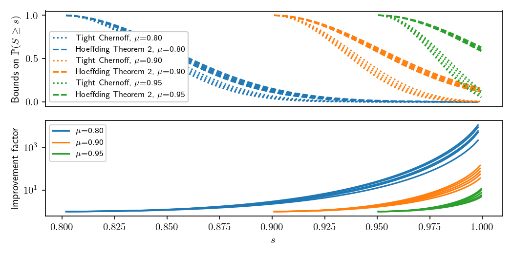
Figure 1: The tightest Chernoff-Cramér bounds are tighter than Hoeffding’s inequality. We consider three choices of fixed mean, $\mu\in\{.8,.9..95\}$, and five randomly selected choices for the subexperiment sizes. We compare tail bounds based on Hoeffding’s inequality (Hoeffding, 1963, Theorem 2) with the tightest Chernoff-Cramér bounds, calculated using Theorem 2 and Theorem 3. The left plot shows the bounds. The right plot demonstrates the factor of improvement, showing ratios of the two bounds on a log scale.

2.4 Error control

We now seek to perform error control, i.e., to estimate a subset of parameters $\mathcal{S}$ such that the type S error proportion among $\{\hat{y}_{i}\}_{i\in\mathcal{S}}$ is low. To do so, we first observe that the CSEP and CSER are well-defined for any subset of parameters $\mathcal{S}\subset\{1,\ldots,n\}$. We denote the corresponding values as $\mathrm{CSEP}_{\mathcal{S}}(\boldsymbol{Y};\boldsymbol{\hat{y}})$ and $\mathrm{CSER}_{\mathcal{S}}(\boldsymbol{\hat{y}})$. Under the conditions of Theorem 1, the type S error proportion of the proposal selections among $\mathcal{S}$ is bounded by $2\cdot\mathrm{CSER}_{\mathcal{S}}(\boldsymbol{\hat{y}})$.

We therefore propose the following approach to error control. Given a sequence of nested candidate subsets $\mathcal{S}_{1}\subset\mathcal{S}_{2}\subset\ldots\subset\mathcal{S}_{K}$, we obtain a quantity $U_{k}$ estimating the $\mathrm{CSER}_{\mathcal{S}_{k}}$ for each $k\in\{1,2,\ldots,K\}$. For any target type S error proportion $V^{*}$, we let $k^{*}$ denote the largest value such that $U_{k}\leq V^{*}/2$ and take our subset to be $\mathcal{S}^{*}=\mathcal{S}_{k^{*}}$.

This approach requires us to specify two ingredients: the candidate subsets and the CSER estimator. To aid us in specifying the candidate subsets, we assume certain auxiliary information is available that indicaties a level of uncertainty about each proposal selection. For example, if a proposal selection $\hat{y}_{i}$ is based on a previous experiment, it may have an associated $p$-value for the null hypothesis that $\theta_{i}=0$. We denote the uncertainty value for parameter $i$ as $\rho_{i}\in\mathbb{R}$. These uncertainty values do not need to be valid $p$-values; $\boldsymbol{\hat{y}}$ and $\boldsymbol{\rho}$ are considered arbitrary deterministic quantities.

We consider three ways to specify these ingredients. Some lead to larger subsets, and some have more rigorous guarantees.

The first way is as follows. Assume, without loss of generality, that the parameters are sorted with respect to $\rho$, i.e., $\rho_{1}\leq\ldots\leq\rho_{n}$. For each $k$, take $\mathcal{S}_{k}=\{1,2,\ldots,k\}$. Take $U_{k}=\mathrm{CSEP}_{\mathcal{S}_{k}}$, which is an unbiased point estimator for $\mathrm{CSER}_{\mathcal{S}_{k}}$.

The second way is more conservative. Take the same candidate subsets used in the first way, but estimate the CSER as the upper bound of a $(1-\alpha)$ confidence interval on $\mathrm{CSER}_{\mathcal{S}_{k}}$. This incorporates our uncertainty.

The third way guarantees error control, with high probability. Instead of sorting parameters by uncertainty, we sort the subexperiments by their average uncertainty:

$$i\leq j\implies\frac{1}{|P_{i}|}\sum_{i}\rho_{i}\leq\frac{1}{|P_{i}|}\sum_{i}\rho_{i}.$$

For each $k$, we then take $\mathcal{S}_{k}$ to be the union of $\{P_{1},P_{2},\ldots P_{k}\}$. We then take $\boldsymbol{U}\in[0,1]^{m}$ to be the upper bounds of a simultaneous $(1-\alpha)$ confidence region for $(\mathrm{CSER}_{\mathcal{S}_{1}},\ldots,\mathrm{CSER}_{\mathcal{S}_{m}})$. Using this option, with probability $(1-\alpha)$, under the conditions of Theorem 1, the type S error proportion of the proposal selections among $\mathcal{S}_{k}$ is less than $2U_{k}$ for all $k$. The construction of the simultaneous confidence region is straightforward because the candidate subsets are defined in terms of the subexperiments. We may therefore use the submartingale inequality to construct the needed confidence region, as the following theorem shows.

Theorem 4.

Fix $\alpha\in[0,1]$. Let $a_{i}=|P_{i}|$ . Let $\varphi^{*}$ be given by Equation 2. Let $\mathcal{S}_{k}=\cup_{i=1}^{k}P_{i}$. Let

$$\hat{s}(\mu)=\max\left\{s:\ \varphi_{\boldsymbol{a},\mu}(s)\leq\alpha\right\}$$

and

$$\delta(s)=\max_{\mu:\varphi_{\boldsymbol{a},\mu}(s)\geq\alpha}\left(\hat{s}(\mu)-\mu\right).$$

Let

$$U_{k}=\mathrm{CSEP}_{\mathcal{S}_{k}}+\frac{\left|\mathcal{S}_{m}\right|}{\left|\mathcal{S}_{k}\right|}\left(\left|\mathcal{S}_{m}\right|-\delta\left(\left(1-\mathrm{CSEP}_{\mathcal{S}_{m}}\right)\left|\mathcal{S}_{m}\right|\right)-\mathrm{CSEP}_{\mathcal{S}_{m}}\right).$$

Then $\mathbb{P}(\mathrm{CSER}_{k}\leq U_{k}\ \forall k)\geq 1-\alpha$.

In Theorem 4, the upper bound $U_{m}$ is identical to the bound that would be obtained by computing a one-sided confidence interval for $\mathrm{CSER}_{\mathcal{S}_{m}}$ by applying Theorem 2 directly. That is, the simultaneous confidence region for $(\mathrm{CSER}_{\mathcal{S}_{1}},\ldots,\mathrm{CSER}_{\mathcal{S}_{m}})$ gives the same bounds on $\mathrm{CSER}_{\mathcal{S}_{m}}$ as a single confidence interval on $\mathrm{CSER}_{\mathcal{S}_{m}}$. This is a typical result when applying submartingale inequalities with Chernoff-Cramér bounds. On the other hand, the bounds $U_{k}$ for $k<m$ are looser than those that would be obtained by constructing a confidence interval for $\mathrm{CSER}_{\mathcal{S}_{k}}$ alone. Indeed, inspecting the equation for $U_{k}$, we observe that the ratio $|\mathcal{S}_{m}|/|\mathcal{S}_{k}|$ becomes large when $|\mathcal{S}_{k}|\ll|\mathcal{S}_{m}|$.

Note that any method for estimating the CSER can be combined with arbitrary preprocessing of the parameter sets based on $\boldsymbol{\rho}$. We give three representative examples. First, for each subexperiment, we could ignore all but the ten parameters with least uncertainty. We could then apply any of the error control options described above. Second, we could sort subexperiments by average uncertainty and discard the second half of subexperiments. Third, if each uncertainty value $\rho_{i}$ were approximately superuniform under the null hypothesis $\theta_{i}=0$, we could ignore parameters $i$ where $\rho_{i}\geq V^{*}$. In general, because $\boldsymbol{\rho}$ is considered deterministic (or, equivalently, conditioned upon), any such preprocessing would not interfere with the type S error guarantees.

3 Case studies

To probe the advantages and limitations of model-free error assessment and control, we conduct two case studies based on cell-perturbation experiments. In the first case study, CSER is used to validate a new method for preprocessing cell-perturbation measurements (Section 3.1). We use the CSER to rigorously show that the new preprocessing method leads to improvements in error control. In the second case study, a CSER-based error control method identifies more discoveries than a model-based error control method (Section 3.2).

3.1 Error assessment

L1000 is a protocol developed by Subramanian et al. (2017) for perturbing cells with small molecules and measuring their resulting gene expression. The protocol involves collecting real-valued fluorescence measurements for each collection of cells. The protocol defines an algorithm for estimating gene expression from these values. We will refer to this method as L1000A. Qiu et al. (2020) developed a new algorithm for reanalyzing the same fluorescence measurements. We will refer to this new method as L1000B. We seek to assess which method yields more accurate results.

Assuming both protocols have correctly specified models, the L1000A method appears superior. For each parameter of interest $\theta_{i}$, both methods produce an estimate $\hat{\theta}_{i}$. In both cases, measurement noise is presumed to be normal and the scale of the each parameter is normalized by an estimate of the measurement error such that $\hat{\theta}_{i}\sim\mathcal{N}(\theta_{i},1)$. The sign of $\theta_{i}$ can thus be estimated by using the sign of $\hat{\theta}_{i}$, and this estimator will have a lower chance of committing a type S error when the magnitude of $\theta_{i}$ is large. We used this model, together with Benjamini-Hochberg (BH), to select a subset of parameters such that the expected Type S error proportion is controlled within that subset (Benjamini and Yekutieli, 2005). Applied to a single experimental replicate with a target Type I error rate of 10%, this procedure yields 138,009 selected parameters from the L1000A data and zero selected parameters from the L1000B data. This suggests that the original L1000A method may be more useful for making discoveries about the parameters of interest. However, these applications of BH are only valid if the measurement error was correctly assessed by both methods.

To justify the use of L1000B, the authors (Qiu et al., 2020) noted that L1000B yielded more consistent answers across experimental replicates. This suggests that the measurement noise may have been incorrectly assessed in at least one protocol. However, those authors did not have a rigorous way to connect their observation about estimator replicability with a notion of estimator error. Theorem 1 provides the necessary link. They also had no way to show that the differences in consistency were above a level to be expected from chance. Theorem 2 allows us to see that the differences were indeed statistically significant.

We begin by computing the CSEP for both L1000A and L1000B. The data contains three replicates; we used two replicates to generate our proposal selections and the final replicate for the validation selections. See Appendix A for additional details on how these values were constructed.

We find that the CSEP in L1000A is 40% and the CSEP in L1000B is 38%. These values are above 25%, and so the bounds of Theorem 1 yield trivial results for both, i.e., type S error proportions in excess of 50%. Because CSEP only implies upper bounds on error proportions, it is conceivable that the type S error proportions are in fact low for both. Nonetheless, it will be difficult to trust that most of these parameters have been estimated correctly if we cannot furnish any evidence of a low error rate. These high CSEP values are consistent with a recent work challenging the average accuracy of the estimates in L1000A (Lim and Pavlidis, 2021).

Although the overall accuracy of both may be poor, there are subsets of parameters where L1000B appears to have acceptable error rates. For each protocol, we obtain an uncertainty value $\rho_{i}$ for each parameter $\theta_{i}$ by taking the negative magnitude of the estimate $\hat{\theta}_{i}$. Crucially, this uncertainty value does not depend upon the validation selections. As discussed in Section 2.4, we are thus free to use $\boldsymbol{\rho}$ to define subsets of parameters and to re-estimate the CSER for these subsets; Theorem 1 remains valid for each subset. For this case study, we consider subsets of the form $\mathcal{S}_{t}=\{i:\rho_{i}\leq t\}$. For each $t$, for each protocol, we compute $\mathrm{CSEP}_{S_{t}}$ along with a 95% two-sided confidence interval for $\mathrm{CSEP}_{S_{t}}$. The confidence intervals are produced using Theorem 2. Each stimuli corresponds to one subexperiment, i.e., we assume the disagreements between $\boldsymbol{\hat{y}}$ and $\boldsymbol{Y}$ for parameters regarding each stimulus are independent of the disagreements concerning other stimuli. Note that these confidence intervals are not simultaneous over $t$.

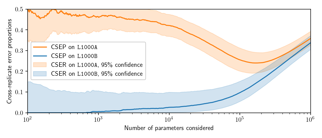
Figure 2: The CSER shows lower error proportions in the estimates of a new protocol. For each threshold $t$, for both the L1000A and L1000B protocols, we estimate the CSER on the subset of parameters whose uncertainty values are less than $t$. We then plot the subset sizes against the corresponding CSER estimates, sweeping over all thresholds. To estimate the CSER, we take the CSEP as a point estimate and use Theorem 2 to produce a 95% two-sided confidence interval. At each fixed number of parameters, we find that L1000B yields lower CSER estimates.

Sweeping over a variety of thresholds $t$, Figure 2 plots the number of parameters in each subset, $|\mathcal{S}_{t}|$, against the corresponding values of $\mathrm{CSEP}_{\mathcal{S}_{t}}$. For example, in L1000B we find a subset of 100,000 parameters with CSEP of 5%, suggesting a type S error proportion below 10%. On the other hand, nontrivial error bounds cannot be identified for L1000A on any subset of data. Moreover, the greatest CSEPs in the L1000A data appear among subsets of parameters with the least uncertainty. This is somewhat surprising, as we might expect estimators with low uncertainty to have lower errors. This evidence supports the conjecture from Qiu et al. (2020) that a small proportion of the fluorescence measurements include profound anomalies, and that the original heuristic algorithm overestimates effect sizes and underestimates error levels in these anomalous readings.

Figure 2 also indicates 95% confidence intervals for $\mathrm{CSER}_{\mathcal{S}_{t}}$ for each $t$, computed using Theorem 2. Such intervals could also have been computed using Hoeffding’s inequality, but the resulting confidence intervals would be broader than necessary by a factor of $3/2$. For example, considering the subset of parameters $\mathcal{S}_{t}$ with 5000 parameters in total, the CSEP is 2.0%, Theorem 2 yields an upper bound of 9.6% for the $\mathrm{CSER}_{\mathcal{S}_{t}}$, whereas the Hoeffding inequality yields an upper bound of 14.2%.

3.2 Error control

In the preceding section we found that nontrivial type S error bounds could be found in L1000B data when we restricted our attention to subsets of the parameters. These subsets were chosen by considering various thresholds on uncertainty values associated with the proposal selections. This suggests it may be possible to obtain a subset of parameters $\mathcal{S}^{*}$ for which the type S error is well-controlled. We now pursue this possibility, applying the error control methods outlined in Section 2.4.

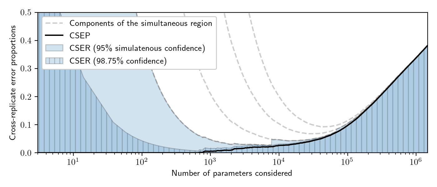
Figure 3: Simultaneous confidence intervals for the CSER in different subsets of parameters. For each threshold $t$, we estimate the CSER on the subset of parameters whose uncertainty values are less than $t$. We then plot the subset sizes against the corresponding CSER estimates, sweeping over all thresholds. In estimating CSER, we consider three possibilities: CSEPs, 98.75% one-sided (non-simultaneous) confidence intervals, and a 95% one-sided confidence region which is simultaneous over all thresholds considered. The last is formed by merging 4 simultaneous 98.75% one-sided confidence regions, the upper bounds of which are plotted with dotted gray lines.

We construct a nested sequence of subsets, with each subset defined by selecting parameters whose uncertainty values lie below a threshold. We consider three approaches to estimate the CSER in each of these subsets. The first approach uses the CSEP for each subset. The second uses a non-simultaneous one-sided 98.75% confidence interval for each subset. The third applies Theorem 4 to yield a 95% simultaneous confidence region. In particular, we choose four thresholds by uniformly spacing five values between the minimum observed uncertainty value and the maximum observed uncertainty value and discarding the first value. For each threshold, we discard parameters whose uncertainty values are greater than the threshold and construct a simultaneous 98.75% confidence region using Theorem 4. The regions are then combined via a union bound. In all cases, we assume that each subexperiment includes only one parameter, i.e., the disagreements between the proposal selections and the validation selections are all independent indicator variables. As in the previous case study (Section 3.1), we use two replicates for producing proposal selections and one replicate for producing validation selections.

Figure 3 shows how different estimates of the CSER lead to selecting different subsets of parameters. For example, suppose we target a type S error proportion of 10%. Taking the CSEPs as our estimates yields a subset of 40,416 parameters with CSEP less than 5%. Thus, 10% is a reasonable estimate of an upper bound for the type S error proportion among these parameters. Using the upper bounds of the 98.75% one-sided confidence intervals for the CSERs would lead to a more conservative conclusion, as we must reduce the number of parameters considered to 35,502 before finding a subset for which this upper bound falls below 5%. Finally, using only the most rigorous estimates available yields a subset of 31,284 parameters for which the 95% simultaneous confidence region indicates that the CSER lies below 5%.

How do these CSER-based approaches to error control compare with model-based methods? We applied BH to a combination of all three replicates of the L1000B data. Under the protocol’s model, the estimators from each replicate are independent, unbiased, and normally distributed with unit variance. We therefore summed the estimators across the replicates, divided by $\sqrt{3}$, and applied Definition 6 of Benjamini and Yekutieli (2005) to the resulting values to identify a subset of parameters where the expected type S error proportion was controlled. This approach yielded a subset of only 24,629 parameters—fewer than the number of parameters identified by even the most conservative CSER-based approach. This could be due to inherently conservative behavior in the BH procedure, but we conjecture that it is also due to overestimated measurement noise levels in the L1000B data.

4 Conclusions

This work proposes a model-free approach for assessing and controlling type S error in high-throughput experiments. Accurate type S error assessment is useful for many reasons. It enables practitioners to control the error, allowing them to identify which results are worthy of future investigation. It enables practitioners to compare the error of different protocols to determine their relative merits. Finally, it enables practitioners to recognize that error rates may be larger than supposed. For example, although the original L1000 data was published in 2017, it took four years for concerns about its replicability to rise to the level of a publication (Lim and Pavlidis, 2021). If the original experimentalists had calculated the CSEP, some of these issues could have been identified immediately. Developing and implementing protocol-specific strategies to evaluate error is difficult. Simple best practices for assessing error that can be applied across experimental modalities would alleviate this burden.

Acknowledgements. We thank Prayag Chatha, Roman Kouznetsov, Declan McNamara, Yash Patel, Cheng Wang, and Mallory Wang for reviewing this manuscript and providing thoughtful comments.

Funding. This research was funded by Immunai Inc.

Appendix A Dataset acquisition and pre-processing

In this work we use two datasets, which we refer to as L1000A and L1000B.

The L1000 dataset was originally presented by Subramanian et al. [2017]. It can be viewed at several levels of pre-processing; we elected to view after it had been preprocessed to what is referred to as “level 4.” The data in this level comprises a $z$-score for each replicate for each perturbation for each dosage for each cell type for each gene. The data can be downloaded from GEO accession GSE70138 (cf. https://www.ncbi.nlm.nih.gov/geo/query/acc.cgi).

This dataset was reanalyzed by Qiu et al. [2020], leading to an alternative dataset, also containing $z$-scores. This data is available from https://github.com/njpipeorgan/L1000-bayesian.

Both datasets include information about 978 genes for many different perturbations applied to many different cell-types at many different dosages. In this work we focus on the parameters concerning A375 cells when subjected to the highest dosages considered for each perturbation.

Appendix B Proofs

B.1 Theorem 1

Observe that

$$\mathrm{CSER} =\frac{1}{n}\left(\sum_{i:\ \hat{y}_{i}=\mathrm{sign}(\theta_{i})}\mathbb{P}\left(Y_{i}\neq\hat{y}_{i}\right)+\sum_{i:\ \hat{y}_{i}\neq\mathrm{sign}(\theta_{i})}\mathbb{P}\left(Y_{i}\neq\hat{y}_{i}\right)\right)$$

$$=\frac{1}{n}\left(\sum_{i:\ \hat{y}_{i}=\mathrm{sign}(\theta_{i})}\mathbb{P}\left(Y_{i}\neq\mathrm{sign}\left(\theta_{i}\right)\right)+\sum_{i:\ \hat{y}_{i}\neq\mathrm{sign}(\theta_{i})}\mathbb{P}\left(Y_{i}=\mathrm{sign}\left(\theta_{i}\right)\right)\right)$$

$$\geq\frac{1}{n}\left(0+\sum_{i:\ \hat{y}_{i}\neq\mathrm{sign}(\theta_{i})}\frac{1}{2}\right)$$

$$=V(\hat{\boldsymbol{y}},\boldsymbol{\theta})/2.$$

B.2 Theorem 2

B.2.1 Topology of the domain

To prove Theorem 2, we view $\mathcal{M}_{\boldsymbol{a},\mu}$ as a topological vector space. For any scalar $b\geq 0$, let $\mathcal{M}_{b}$ denote the space of probability measures with support on $[0,b]$. Endowing $\mathcal{M}_{b}$ with the weak-$*$ topology, we view $\mathcal{M}_{b}$ as a topological vector space. Note that $\mathcal{M}_{b}$ is compact and convex. For any subexperiment sizes $\boldsymbol{a}\in({\mathbb{R}^{+}})^{m}$ and fixed mean $\mu$, let

$$\mathcal{M}_{\boldsymbol{a},\mu}=\left\{\boldsymbol{p}\in\prod_{i}\mathcal{M}_{a_{i}}:\ \sum_{i}\mathbb{E}_{X_{i}\sim p_{i}}[X_{i}]\leq\mu\right\}.$$

Here

$$\prod_{i}\mathcal{M}_{a_{i}}$$

denotes a direct sum of a topological vector spaces. For example, if $\boldsymbol{p}\in\mathcal{M}_{\boldsymbol{a},\mu}$ then $\boldsymbol{p}=(p_{1},\ldots p_{m})$ where each $p_{i}\in\mathcal{M}_{a_{i}}$. For any $\boldsymbol{p},\boldsymbol{q}\in\mathcal{M}_{\boldsymbol{a},\mu}$, $(\boldsymbol{p}+\boldsymbol{q})/2=((p_{1}+q_{1})/2,\ldots(p_{m}+q_{m})/2)$. Note that $\mathcal{M}_{\boldsymbol{a},\mu}$ is convex.

B.2.2 Proof

Fix $s$. Let

$$f(t,\boldsymbol{p})=\sum_{i}\log\mathbb{E}_{X_{i}\sim p_{i}}[\exp(tX_{i})]-ts.$$

Our object of interest is may be given as $\min_{t}\max_{\boldsymbol{p}}f(t,\boldsymbol{p})$. Our first step is to reverse the order of the minimization and maximization by applying Sion’s minimax theorem. We observe the following.

• $f$ is convex with respect to $t$, as it is the sum of cumulant generating functions.

• $f$ is concave with respect to $\boldsymbol{p}$, due to Jensen’s inequality.

• $f$ is continuous with respect both $\boldsymbol{p}$ and $t$.

• $\mathcal{M}_{\boldsymbol{a},\mu}$ is both convex and compact.

• $[0,\infty)$ is convex (though not compact).

Sion’s minimax theorem thus shows that

$$\min_{t\geq 0}\max_{\boldsymbol{p}\in\mathcal{M}_{\boldsymbol{a},\mu}}f(t,\boldsymbol{p})=\min_{t\geq 0}\max_{\boldsymbol{p}\in\mathcal{M}_{\boldsymbol{a},\mu}}f(t,\boldsymbol{p}).$$

For any fixed $t$, the maximization of $f$ may be reduced to a finite-dimensional problem. First, we rewrite the maximization problem by introducing auxiliary variables, as follows:

$$\max_{\boldsymbol{p},\tau}\qquad f(t,\boldsymbol{p})$$

$$\mathrm{s.t.}\qquad \tau_{i}\in[0,a_{i}]$$

$$p_{i}\in\mathcal{M}_{a_{i}}$$

$$\tau_{i}=\sum_{i}\mathbb{E}_{X_{i}\sim p_{i}}\left[X_{i}\right]$$

$$\sum_{i}\tau_{i}\leq\mu$$

For any fixed $\tau$, Hoeffding [Hoeffding, 1963, proof of Theorem 1] showed that the cumulant generating functions can be maximized by setting each $p_{i}$ to be a scaled Bernoulli random variable, namely

$$p_{i}=\delta_{0}\left(1-\frac{\tau_{i}}{a_{i}}\right)+\delta_{a_{i}}\frac{\tau_{i}}{a_{i}}$$

where $\delta_{x}$ represents the point mass at $x$. Under this distribution,

$$\log\mathbb{E}_{p_{i}}\left[\exp\left(tX_{i}\right)\right]=\log\left(1+\xi(a_{i},t)\tau_{i}\right).$$

Note that this is monotone increasing in $\tau$, so the constraint $\sum_{i}\tau_{i}\leq\mu$ may be replaced with the constraint $\sum_{i}\tau_{i}=\mu$ without changing the result. Our problem thus reduces to the desired form.

B.3 Theorem 3

For any fixed $t\geq 0$, we begin by rewriting the maximization problem in terms of

$$f(\tau;t)=\begin{cases}\sum_{i}\log\left(1+\xi(a_{i},t)\tau_{i}\right)-ts&\mathrm{if}\ \tau\in\prod_{i}[0,a_{i}]\\ -\infty&\mathrm{else}.\end{cases}$$

That is, we incorporate the inequality constraints into the domain of optimization. The maximization problem of interest is equivalent to

$$\max_{\tau:\ \sum_{i}\tau_{i}=\mu}f(\tau;t).$$

The associated Lagrangian function is given by

$$\mathcal{L}(\tau,\lambda;t)=\sum_{i}\log\left(1+\xi(a_{i},t)\tau_{i}\right)+\lambda\left(\mu-\sum_{i}\tau_{i}\right)-ts.$$

For any fixed $t\geq 0$, observe that $\xi(a_{i},t)$ is positive and thus $\tau\mapsto\mathcal{L}\left(\tau,\lambda;t\right)$ is concave. The argument maximizing $\tau\mapsto\mathcal{L}(\tau,\lambda;t)$ is given by $\tau_{i}^{*}(t,\lambda)$. Thus $g(t,\lambda)=\max_{\tau}\mathcal{L}(\tau,\lambda;t)$, the Lagrangian dual for a convex optimization problem with convex constraints. There is at least one feasible point, namely $\tau_{i}=a_{i}\mu/\sum_{j}a_{j}$, so strong duality holds and

$$\max_{\begin{subarray}{c}\tau\in\prod_{i}[0,a_{i}]\\ \sum_{i}\tau_{i}=\mu\end{subarray}}\sum_{i}\log\left(1+\xi(a_{i},t)\tau_{i}\right)-ts=\min_{\lambda}g(t,\lambda)$$

as desired.

We now demonstrate that $g$ is convex. First, observe that $\mathcal{L}$ is affine in $\lambda$ and convex in $t$. Thus $g$ is a pointwise maximum of a family of convex functions: it is convex.

Finally, we demonstrate that $t\mapsto\min_{\lambda}g(t,\lambda)$ is convex. Observe that, for any fixed $\tau_{i}\geq 0$, the mapping

$$t\mapsto\sum_{i}\log\left(1+\xi(a_{i},t)\tau_{i}\right)-ts$$

is convex in $t$. Thus $\min_{\lambda}g(t,\lambda)$ is also the pointwise maximum of a family of convex functions: it is also convex.

B.4 Theorem 4

Let $S_{k}=\sum_{i=1}^{k}\left(a_{i}-X_{i}\right)$. We will first construct a simultaneous confidence interval on $\mu_{k}\triangleq\mathbb{E}\left[S_{k}\right]$; simultaneous confidence intervals on the corresponding CSERs will then be straightforward to obtain. Let

$$C(\boldsymbol{S})=\left\{\hat{\boldsymbol{\mu}}:\ \hat{\mu}_{k}\geq S_{k}-\hat{s}(\hat{\mu}_{m})+\hat{\mu}_{m}\ \forall k\right\}.$$

a confidence region for $\boldsymbol{\mu}$. What is its coverage probability? Observing that $\left(S_{1}-\mu_{1},S_{2}-\mu_{2},\ldots S_{m}-\mu_{m}\right)$ is a martingale and applying the submartingale inequality, we find that

$$\mathbb{P}\left(\boldsymbol{\mu}\notin C(\boldsymbol{S})\right) =\mathbb{P}\left(S_{k}-\hat{\mu}_{k}>\hat{s}(\hat{\mu}_{m})-\hat{\mu}_{m}\ \forall k\right)$$

$$\leq\inf_{t\geq 0}\mathbb{E}\left[\exp\left(t\left(S_{m}-\mu_{m}\right)-t\left(\hat{s}\left(\hat{\mu}_{m}\right)-\hat{\mu}_{m}\right)\right)\right]=\varphi_{\boldsymbol{a},\mu_{m}}^{*}\left(\hat{s}\left(\hat{\mu}_{m}\right)\right)\leq\alpha.$$

Thus $C(\boldsymbol{S})$ is an $\alpha$-valid confidence interval for $\mu_{k}$.

The definition of $C$ is unwieldy, as the bound on each parameter $\hat{\mu}_{k}$ is expressed in terms of a nontrivial function of the parameter $\hat{\mu}_{m}$. We can obtain a slightly larger confidence region by calculating an overall lower bound for each individual parameter. Letting

$$\hat{\mu}_{k}^{*}(\boldsymbol{S})\triangleq\min_{\hat{\boldsymbol{\mu}}\in C(\boldsymbol{S})}\hat{\mu}_{k} =S_{k}-\max_{\hat{\boldsymbol{\mu}}\in C(\boldsymbol{S})}\left(\hat{s}\left(\hat{\mu}_{m}\right)-\hat{\mu}_{m}\right)$$

$$=S_{k}-\max_{\hat{\mu}_{m}:\ \hat{\mu}_{m}\geq S_{m}-\hat{s}(\hat{\mu}_{m})+\hat{\mu}_{m}}\left(\hat{s}\left(\hat{\mu}_{m}\right)-\hat{\mu}_{m}\right)$$

$$=S_{k}-\max_{\hat{\mu}_{m}:\ \hat{s}(\hat{\mu}_{m})\geq S_{m}}\left(\hat{s}\left(\hat{\mu}_{m}\right)-\hat{\mu}_{m}\right)$$

$$=S_{k}-\max_{\hat{\mu}_{m}:\ \varphi_{\boldsymbol{a},\mu}(s)\geq\alpha}\left(\hat{s}\left(\hat{\mu}_{m}\right)-\hat{\mu}_{m}\right),$$

we are guaranteed that

$$\mathbb{P}\left(\hat{\mu}_{k}\geq\hat{\mu}_{k}^{*}\left(\boldsymbol{S}\right)\ \forall k\right)\geq 1-\alpha.$$

Finally, to calculate lower bounds on our objects of interest we recall that

$$\mathrm{CSEP}_{\mathcal{S}_{k}} =1-S_{k}/\left|\mathcal{S}_{k}\right|$$

$$\mathrm{CSER}_{\mathcal{S}_{k}} =1-\hat{\mu}_{k}/\left|\mathcal{S}_{k}\right|.$$

Substituting these into the definition of $\hat{\boldsymbol{\mu}}^{*}(\boldsymbol{S})$, we obtain our final result.

References

- Benjamini and Yekutieli [2005] Yoav Benjamini and Daniel Yekutieli. False Discovery Rate–Adjusted Multiple Confidence Intervals for Selected Parameters. Journal of the American Statistical Association, 100(469):71–81, March 2005.
- Chen et al. [2016] Mengjie Chen, Zhao Ren, Hongyu Zhao, and Harrison Zhou. Asymptotically normal and efficient estimation of covariate-adjusted gaussian graphical model. Journal of the American Statistical Association, 111(513):394–406, 2016.
- Davidson [2001] E.H. Davidson. Genomic Regulatory Systems: In Development and Evolution. Elsevier Science, 2001.
- Gelman and Tuerlinckx [2000] Andrew Gelman and Francis Tuerlinckx. Type S error rates for classical and Bayesian single and multiple comparison procedures. Computational Statistics, 15(3):373–390, 2000.
- Hoeffding [1963] Wassily Hoeffding. Probability Inequalities for Sums of Bounded Random Variables. Journal of the American Statistical Association, 58(301):13–30, 1963.
- Lim and Pavlidis [2021] Nathaniel Lim and Paul Pavlidis. Evaluation of connectivity map shows limited reproducibility in drug repositioning. Scientific Reports, 11(1):1–14, 2021.
- Qiu et al. [2020] Yue Qiu, Tianhuan Lu, Hansaim Lim, and Lei Xie. A Bayesian approach to accurate and robust signature detection on LINCS L1000 data. Bioinformatics, 36(9):2787–2795, 2020.
- Schmidt et al. [2022] Ralf Schmidt, Zachary Steinhart, Madeline Layeghi, Jacob W Freimer, Raymund Bueno, Vinh Q Nguyen, Franziska Blaeschke, Chun Jimmie Ye, and Alexander Marson. CRISPR activation and interference screens decode stimulation responses in primary human T cells. Science, 375(6580), 2022.
- Shi et al. [2022] Bowen Shi, Yanyuan Wu, Haojie Chen, Jie Ding, and Jun Qi. Understanding of mouse and human bladder at single-cell resolution: integrated analysis of trajectory and cell-cell interactive networks based on multiple scRNA-seq datasets. Cell Proliferation, 55(1):e13170, 2022.
- Srivatsan et al. [2020] Sanjay R Srivatsan, José L McFaline-Figueroa, Vijay Ramani, Lauren Saunders, Junyue Cao, Jonathan Packer, Hannah A Pliner, Dana L Jackson, Riza M Daza, Lena Christiansen, et al. Massively multiplex chemical transcriptomics at single-cell resolution. Science, 367(6473):45–51, 2020.
- Stein et al. [2015] Caleb K Stein, Pingping Qu, Joshua Epstein, Amy Buros, Adam Rosenthal, John Crowley, Gareth Morgan, and Bart Barlogie. Removing batch effects from purified plasma cell gene expression microarrays with modified combat. BMC Bioinformatics, 16(1):1–9, 2015.
- Subramanian et al. [2017] Aravind Subramanian, Rajiv Narayan, Steven M Corsello, David D Peck, Ted E Natoli, Xiaodong Lu, Joshua Gould, John F Davis, Andrew A Tubelli, Jacob K Asiedu, et al. A next generation connectivity map: L1000 platform and the first 1,000,000 profiles. Cell, 171(6):1437–1452, 2017.
- Wang et al. [2022] Lina Wang, Yongjun Piao, Dongyue Zhang, Wenli Feng, Chenchen Wang, Xiaoxi Cui, Qian Ren, Xiaofan Zhu, and Guoguang Zheng. FBXW11 impairs the repopulation capacity of hematopoietic stem/progenitor cells. Stem Cell Research & Therapy, 13(1):1–14, 2022.
- Wu and Luo [2022] Qiuyu Wu and Xiangyu Luo. Estimating heterogeneous gene regulatory networks from zero-inflated single-cell expression data. The Annals of Applied Statistics, 16(4):2183 – 2200, 2022.
- Xie et al. [2022] Shishuai Xie, Wanxiang Niu, Feng Xu, Yuping Wang, Shanshan Hu, and Chaoshi Niu. Differential expression and significance of miRNAs in plasma extracellular vesicles of patients with Parkinson’s disease. International Journal of Neuroscience, 132(7):673–688, 2022.
- Yoon et al. [2022] Sojung Yoon, Sung Eun Kim, Younhee Ko, Gwang Hun Jeong, Keum Hwa Lee, Jinhee Lee, Marco Solmi, Louis Jacob, Lee Smith, Andrew Stickley, et al. Differential expression of microRNAs in Alzheimer’s disease: A systematic review and meta-analysis. Molecular Psychiatry, 27(5):2405–2413, 2022.