Sniffer deployment in urban area for human trajectory reconstruction and contact tracing

Abstract

To study the propagation of information from individual to individual, we need mobility datasets. Existing datasets are not satisfactory because they are too small, inaccurate or target a homogeneous subset of population. To draw valid conclusions, we need sufficiently large and heterogeneous datasets. Thus we aim for a passive non-intrusive data collection method, based on sniffers that are to be deployed at some well-chosen street intersections. To this end, we need optimization techniques for efficient placement of sniffers. We introduce a heuristic, based on graph theory notions like the vertex cover problem along with graph centrality measures.

I Introduction

Understanding the diffusion of information from individual to individual can provide insights into various fields ranging from the study of opportunistic networks to the spread of diseases. The spread of information or diseases occurs when individuals find themselves in close proximity. We therefore need to trace such contacts which can be infered from mobility data. Indeed, if one knows the trajectories of the individuals, one can infer then contacts between them, that is, a potential propagation.

The lack of usable mobility dataset makes the study of propagation difficult. Several active datasets are available like [9] but the precision provided by the GPS is not sufficient to infer accurate contacts. Sometimes due to measurements errors, an individual may be in a different street than what is reported. Other datasets like [2] only provide small scale data because the data collection is restricted to indoor environments. Other are available but they use an intrusive approach. This implies that only the people that agreed to to be traced can be monitored, thus creating a bias in the data because the recruted population is often homogeneous. This usually corresponds to students at a computer science department or participants at a conference as in [16]. None of these solutions scale easily so they yield only small scale data.

In this paper, we choose to study a passive non-intrusive data collection approach because it can scale easily, provides sufficiently precise data, and may target a heterogeneous population as individuals don’t need to actively report their location. We choose to work with sniffers that detect an individual passing within a certain range. We can not get a full coverage of our target area with our set of sniffers as the cost would be prohibitive, or the target area too small to be relevant. We therefore need to develop optimization techniques to efficiently place such sniffers. To do so, we propose in this paper, a technique based on graph theory notions like the vertex cover problem, along with graph centrality measures. The vertex cover problems allows us to cover each edge, that is, each street section. Then the graph centralities help us pick the most relevant street intersections. To evaluate our solution, we retrieve the road graph of a city for which user trajectories are known, then compute sniffer locations. Then we can measure the performance of our solution by computing how many trajectories are covered. Our experiments show that, on a realistic dataset, monitoring $20\%$ of the street intersections of our target area, we are able to “see” about $95\%$ of the trajectories enough times (i.e. multiple times with regards to the trajectory). In order to illustrate the targeted size, a possible deployment is shown in figure 1, where the red dots represents street intersections where sniffers are deployed.

The remainder of this article is organized as follows: first we describe our system model in section II, then we give a brief reminder on the tools in section III that are used in this article, then we review the related works in section IV. In section V, we explain our heuristic, then in section VI, we list the results based on a realistic mobility dataset.

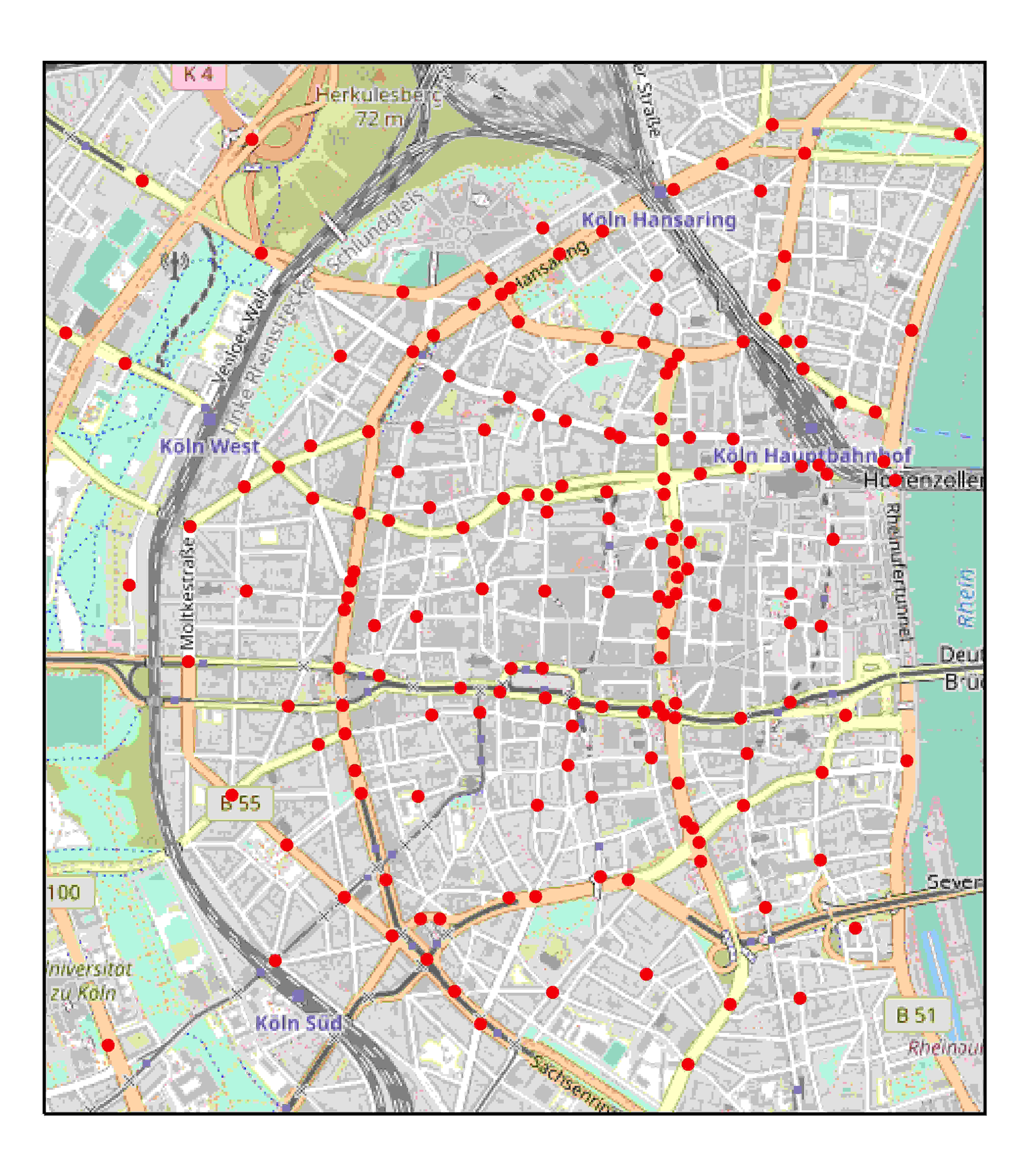
Figure 1: map of downtown Cologne with sniffer deployment example

II System model

II-A Road Networks and trajectories

A graph $G$ consists of a set of vertices $V$ and a set of edges $E\subseteq V\times V$. A graph can represent many things, including road networks: the edges would be street sections and the vertices would be the street intersections. Figure 2 shows an example of a road graph drawn next to its corresponding map.

Working with unweighted distances might not always capture human mobility accurately as an edge can represent either a long or a short street section. Since our road graph represents real world data, it’s not difficult to enrich it with additional information such as the GPS coordinates of our vertices. This allows us to retrieve the real embedding of our graphs, thus to compute the real world distances as the crow flies between vertices.

The map of the targeted area can be retrieved from OpenStreetMap and easily converted into a graph as on figure 2(a). Note that this is a simplified example as more vertices could be added as well as some self loops. Such a representation is not unique. Working with a graph representation allows us to take advantage of a wide range of algorithms and properties already known about graphs.

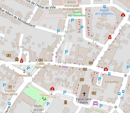
(a) Underlying map

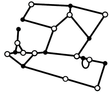
(b) A possible vertex cover

Figure 2: Part of the Cologne road network (left), along with a road graph that models it (right).

A trajectory $T$ is a path in our road graph, i.e., an ordered list of consecutive edges:

$$T=\{((u_{0},u_{1}),(u_{1},u_{2}),\ldots,(u_{k-1},u_{k})),\forall i,(u_{i-1},u_{i})\in E\}$$

The length of a trajectory in an unweighted graph is the number of edges along the trajectory: here the length is $k$.

II-B Problem statement

Our objective is to monitor the least amount of vertices of a road graph, while maximizing the amount of trajectories seen by the sniffers, as well as the amount of time they are seen. Our sniffers have a known range within which it is most likely that wireless activity will be captured. For this reason, we choose to work with the distance as the crow flies between the two endpoints of an edge.

We talk about vertices of a road graph rather than sniffers, because while we aim at working with sniffers deployment in the end, the placement of sniffers within a street intersection is another task in itself as it entails taking into account the topology of the intersection. An intersection might require several sniffers if it is too large or if there is too much traffic. This constraints must be taken into account for a physical deployment of sniffers. In this article, we restrict ourselves to the macroscopic view of sniffer deployment by monitoring vertices in a graph.

III Background: Vertex Cover and graph centrality

Our objective is to select a subset of vertices that are evenly spread out in the graph. This can be done using a Vertex Cover algorithm. Then, to reduce the amount of vertices, we select some of them based on some metrics called Centralities measures. It has been shown that these measures allow an “extended comprehension of the city structure, nicely capturing the skeleton of most central routes” [11].

III-A Vertex Cover

A Vertex Cover is a subset of vertices of a graph that includes at least one endpoint of every edge of the graph. More formally, given a graph $G=(V,E)$, a Vertex Cover is a $S\subseteq V$ such that $\forall(u,v)\in E$, $u\in S$ or $v\in S$. A Minimum Vertex Cover is a set $S$ of minimum size.

Intuitively, if we put sniffers on every vertex of the vertex cover, then we can monitor the whole graph, as every trajectory of length at least one has to go through $S$. Sniffers need to be put where changes of direction happen, because that’s the information we need to reconstruct the shape of the trajectory.

White nodes in Figure 2(b) are an example of a vertex cover: all edges of this graph have a white end. Note that this vertex cover might not be minimum since there are edges for which ends are white. This problem belongs to the 21 problems that were proven NP-complete by Karp in 1972 [19], therefore we often use approximation or heuristic algorithms.

In Maximum $k$-path Vertex Cover problem [22], we are given $s$ sniffers, and we need to maximize the amount of paths of length at least $k$ that go through our at least one sniffer. Formally, given a graph $G=(V,E)$, an integer $k$ and an integer $s$, we want to find $S\subset V$, such that $\left|S\right|\leq s$, maximizing the amount of paths of length at least $k$ covered by $S$.

Few properties are known for this problem. It has been shown [22] that $MaxP_{3}VC\in$ NP-Hard for split graphs, and P for graphs with bounded treewidth, $MaxP_{3}VC\in$ XP with respect to the treewidth ($tw$), $MaxP_{3}VC\in$ FPT with respect to $s$ and $tw$. Finally, $MaxP_{3}VC\in$ P for trees.

III-B Graph centralities

Centralities are values assigned to each node of a graph. They represent how important a node is in a network. We review the main centrality measures from the literature, which are all used in our solution.

1. Degree centrality is defined as the number of edges that are adjacent to a given vertex [5].

2. Strength centrality of a vertex $u$ is the sum of the weights of the adjacent edges of vertex $u$. This is the weighted equivalent of the degree centrality and is also known as the weighted degree centrality [4].

3. Closeness centrality of a vertex $u$ is the inverse of the average length of the shortest path from vertex $u$ to all other vertices in the graph [6].

4. Betweenness centrality of a vertex $u$ is the number of shortest paths which pass through $u$, divided by the number of shortest paths between all pairs of vertices. [12]

5. Katz centrality of a vertex $u$ takes into account the amount of paths of length $k$ starting from $u$, while favouring short paths [20].

6. Eigenvector centrality sums over the neighbours of a vertex just like the degree centrality. It goes a step further by weighting the neighbours based on their own eigenvector centrality. This way, being adjacent to central neighbours makes the vertex more central [23].

7. Information centrality is based on the “information” contained in all possible paths of vertices [25].

8. Accessibility of a vertex $u$ is based on the set of vertices that are reachable by self-avoiding walks of length $h$, starting from $u$ [27].

9. Expected Force aims at modeling the force of infection of a vertex [21].

IV Related Work: Understanding human mobility in urban areas through mobile technologies

There have been different approaches in the literature that tried to use personal mobile devices in order to understand human mobility. Below, we outline the main approaches and their limitation.

Mobility has been studied through an Android application in [9], or through people carying devices in [16]. Those datasets are necessarily restricted by the limited number of people involved in the study, and usually biased as they only target a homogenous subset of people.

K. Akkaya et al. used existing Wi-Fi networks inside buildings to determine which rooms were occupied, based on Received Signal Strength Indication (RSSI) and Media Access Control (MAC) addresses [2]. This is difficult to generalize to outdoor settings as we can not leverage existing Wi-Fi networks in urban areas because public Wi-Fi networks are not broadly available. Another downside is that this only allows to monitor devices connected to a particular Wi-Fi network.

[1] presents a pedestrian counting method based on Fresnel lenses. These lenses leverage the infrared technology to count the pedestrians. This study only counts users, it does not identify them so trajectories cannot be reconstructed and contacts between users cannot be inferred. Plus, the placement strategy is not discussed.

Sniffer placement has been studied in [18] and [7], at a small scale only. Those papers study the impact of sniffer deployment on the localization accuracy, which is computed based on the RSSI. Other studies like [10] and [13] leverage the Wi-Fi technology to monitor the speed and density of road traffic. Those studies are conducted at a large scale, but the sniffer placement strategy isn’t discussed.

In our work, we aim at monitoring human mobility in urban areas in order to allow trajectory reconstruction and contact tracing. Our aim is to avoid any social bias while achieving this. We thus propose to study what an efficient sniffer placement approach, i.e. a passive mobility monitoring approach, would bring to achieve our human mobility monitoring objective.

V Sniffer placement for efficient trajectory reconstruction and contact tracing

As mentioned earlier, the idea we are following for sniffer placement is to start by computing a vertex cover which provides us with a subset of vertices through which all trajectories must go. Then to use the centralities to select the most relevant vertices.

V-A Vertex Cover

There is a 2-approximation algorithm, which according to [24], has been discovered independently by F. Gavril and M. Yannakakis.

In the planar case, that is, when a graph can be embedded in a plane, without having two edges crossing, the Bar-Yehuda and Even’s algorithm [3] is a linear time $\frac{5}{3}$-approximation for the Minimum Vertex Cover Problem. Its bound is slightly better than the 2-approximation algorithm from F. Gavril and M. Yannakakis [24] that also runs in linear time [3].

Note that in a road graph, there can be bridges and other constructions that make it non-planar but a road graph can not be arbitrarily complex because of real world constraints. Even if our road graphs are not necessarily planar, our tests show that, on our road graphs, this algorithm outperforms Gavril and Yannakakis’ 2-approximation algorithm.

V-B Sniffer Placement Heuristic

Our heuristic is built on top of the vertex cover computed with Bar-Yehuda: we perform sniffer placement decisions using Algorithm 1. More precisely, Bar-Yehuda returns a vertex cover $VC$ and the most central node $u$ of $VC$ is kept while all the vertices close to $u$ are removed from $VC$.

In the algorithm, centrality returns a vector of centralities for all vertices in the graph. That is, each node is assigned a value going from $0$ to $1$. Different centralities can be used, such as the ones presented in subsection III-B.

This heuristic also takes as parameters an integer $k$ that influences the distance within which the vertices are pruned from the vertex cover set. Higher values mean more vertices will be pruned, resulting in less street intersections being monitored. A balance can be found between the ratio of uncaught trajectories and the proportion of intersections where sniffers are deployed. The distance within which the vertices are pruned not only depends on $k$ but also on the centrality of $u$ (see line 7 and 8 of the algorithm). The most central vertices will require less pruning since they probably correspond to denser zones where many trajectories are likely to be found. Our experiments show that monitoring more closely areas where central vertices are found allows us to see more trajectories.

Algorithm 1 Sniffer Placement Heuristic (G, k)

1:$VC\leftarrow\textsc{Bar-Yehuda(G)}$

2:$VC_{k}\leftarrow\emptyset{}$

3:cent_vector $\leftarrow\textsc{centrality}(G)$

4:while $VC\neq\emptyset$ do

5:     Pick the most central node $u$ from $VC$

6:     $VC_{k}\leftarrow u$

7:     $c\leftarrow 1-\left(\frac{\textrm{index of }u\textrm{ in }\mathit{cent\_vector}}{\left|V\right|}\right)$

8:     Remove from $VC$, $u$ and all the vertices within distance $\textsc{round}(k\times c)$ of $u$

9:end while

10:return $VC_{k}$

The implementation of these two algorithms is available on [15].

VI Experiments on real datasets

VI-A Datasets

Two datasets are used to analyse the performance of our sniffer placement strategy.

VI-A1 Cologne

This dataset is provided by the TAPAS Cologne project, which aims at reproducing, with the highest level of realism possible, car traffic in the greater urban area of the city of Cologne, Germany. The resulting synthetic trace covers a region of 400 square kilometers for a period of 24 hours in a typical working day. It includes 1 538 464 trajectories. [26] The dataset also includes a map of Cologne.

The map and the trajectories have been extracted with a tool that converts the map into a graph, and the trajectories into an ordered list of edges. It is available on [14].

Since the area included in the TAPAS Cologne project is wider than any realistic deployment, and not homogeneous due to its different areas (urban, non urban, residential) we restrict ourselves to downtown Cologne. We therefore shrink the data to a fourteen square kilometres area, corresponding to what is shown in figure 1

Our restricted dataset contains a road graph with 1080 vertices and 1615 edges, along with 51 695 trajectories that never leave the restricted graph. The length distribution is shown in figure 3.

Figure 3: Distribution of the lengths, in number of street sections, of trajectories in downtown Cologne

VI-A2 Bologna

The Bologna dataset was developed as part of the project iTRETRIS [17]. This is a smaller dataset than Cologne, revolving around two main streets of the city of Bologna. It simulates dense pedestrian movements as observed around football stadiums during big events such as football games or concerts [8]. The road graph of this dataset contains 159 vertices, 215 edges and 11000 trajectories.

VI-A3 Evaluation Methodology

In the future, our goal is to reconstruct user trajectories from incomplete measurements. To this end, we need to adapt our deployment of sniffers in order to maximize the amount of trajectories that we can reconstruct with enough precision. We consider that a trajectory can be reconstructed if it is observed ”often” enough. In what follows, we consider that a trajectory is lost and cannot be reconstructed, using two definitions: (i) when less than $x\%$ of its vertices are monitored or (ii) when it crosses less than $y$ monitored vertices. In the following we use the following values: $x=20\%$, $x=10\%$, $y=4$. These thresholds are purely arbitrary and their impact shall be studied in the future.

VI-A4 Efficiency

Let us now define a measure of efficiency. The goal is to minimize the number of street intersections that we monitor, that is, use the least amount of sniffers, along with minimizing the number of lost trajectories. See equation 1, where $S$ is the number of sniffers, $V$ is the number of vertices in our graph, $L$ is the number of lost trajectories, and $T$ is the number of trajectories in our dataset. We need to maximize this function. This function ranges from $0$ to $1$, with $0$ being the worst and $1$ being the best.

$$\textrm{Efficiency}=\frac{|V|-|S|}{|V|}\times\frac{|T|-|L|}{|T|}$$ (1)

The $k$ value influences the distance within which the vertices are pruned from the vertex cover set. As $k$ grows, the number of sniffers decreases, thus the number of lost trajectories increases. $k$ should be chosen in order to maximize the efficiency, as shown in Figure 4.

Note that table I shows the $k$ value that maximizes the efficiency, which is easy to do since we have a dataset with the trajectories. A way to choose $k$ a priori should be developed.

Figure 4: Efficiency as a function of $k$, for downtown Cologne, with expected force centrality.

VI-A5 Baselines

To put our results into perspective, given that there is no similar work in the state of the art, we also defined several more baselines to evaluate the quality of our results.

The first baseline consists in selecting vertices at random. We choose the number of vertices that gives us the best results on average over 10 runs. Because we pick vertices at random, they should be evenly spread out across our graph. This corresponds to the line “Random” in table I. We expect this method to yield poor results.

We used the strength centrality using a priori knowledge of the trajectories: the weight of each edge is the number of trajectories that go through that edge. The strength centrality of a node $u$ is then the sum of the weight of each of the edges that are adjacent to $u$. This centrality requires a priori knowledge of the trajectories and is expected to outperforms other centralities.

We also implemented four greedy strategies that also use a priori knowledge of the trajectories. “Greedy Lost” chooses, at each step, the unmonitored vertex through which the largest amount of lost trajectories go, until $h$ vertices are chosen. We pick the $h$ that maximizes our efficiency function. “Greedy No Lost” does the same but stops when there is no more lost trajectories. “Greedy Traj” chooses, at each step, the unmonitored vertex through which the largest amount of trajectories go, until $h$ vertices are chosen. Finally, “Greedy No Traj” is the same but stops when $0\%$ of the trajectories are lost.

VI-B Results

VI-B1 Downtown Cologne dataset

We run our heuristic on the road graph of downtown Cologne, with different centrality measures in order to compare their efficiency.

Our results are summarized in table I. The $k$ value is chosen in order to maximize the efficiency function, as explained in Section VI-A4.

Lost	20%				10%				4
Centrality	k	Sniffers	Lost	Efficiency	k	Sniffers	Lost	Efficiency	k	Sniffers	Lost	Efficiency
Strength	9	16.14%	4.10%	0.804	17	10.07%	4.14%	0.862	9	16.14%	8.84%	0.764
Greedy Traj		17.13%	7.77%	0.764		13.89%	5.54%	0.814		17.13%	10.03%	0.746
Greedy No Traj		86.02%	0%	0.140		82.50%	0%	0.172		97.96%	0.60%	0.019
Greedy Lost		16.76%	8.54%	0.761		10.83%	8.84%	0.813		17.41%	10.06%	0.743
Greedy No Lost		85.46%	0%	0.144		82.13%	0%	0.177		97.96%	0.60%	0.019
Degree	5	16.48%	4.54%	0.797	7	13.80%	1.31%	0.851	4	20.56%	7.29%	0.736
Katz	8	18.15%	3.00%	0.794	20	9.54%	4.39%	0.865	8	18.15%	9.21%	0.743
Expected Force	9	17.13%	4.14%	0.794	23	8.98%	5.00%	0.865	9	17.13%	10.70%	0.740
Accessibility	10	15.93%	5.88%	0.791	14	12.31%	2.50%	0.856	9	17.31%	9.82%	0.756
Betweenness	7	20.56%	3.88%	0.764	13	12.96%	3.26%	0.842	7	20.56%	9.02%	0.723
Information	6	20.37%	4.21%	0.763	14	11.02%	4.79%	0.847	10	14.63%	13.52%	0.738
Closeness	4	23.33%	7.10%	0.712	9	13.61%	8.35%	0.792	4	23.33%	10.96%	0.683
Eigenvector	3	27.41%	3.39%	0.701	5	19.72%	3.19%	0.777	4	22.96%	11.32%	0.683
Random	286	26.48%	5.60%	0.696	204	18.89%	4.10%	0.780	258	23.89%	14.12%	0.654

TABLE I: Results for each centrality, on downtown Cologne, considering different lost thresholds.

(a)

(b)

Figure 5: Cologne Downtown, $\emph{lost}=20\%$, strength, $k=9$

The first column of table I considers that a trajectory is lost when less than $20\%$ of the street intersections it crosses are monitored with sniffers. In this column, with most centralities, less than $20\%$ of the vertices need to be monitored to catch more than $95\%$ of the trajectories. This can also be seen on figure 5(a) that show how well observed are the trajectories in terms of monitored nodes.

A deeper inspection shows that the lost trajectories are mostly short ones. The shorter a trajectory, the more unlikely it becomes to monitor $20\%$ of its vertices. For instance we have to put sniffers at every intersection to catch trajectories of length lower than $5$ and we can miss only one intersection for trajectories of length lower than $10$. This is confirmed by Figure 5(b) that represents the amount of lost trajectories as a function of their length. We can see that almost $40\%$ of the trajectories of length $4$ are lost and more generally shorter trajectories tend to have more lost among them.

VI-B2 Impact of Lost

To better understand the impact of the definition of lost, we also consider a trajectory lost when less than $10\%$ of the street intersections it crosses are monitored. The second column of table I shows the results we get when taking into account this new definition. The value of $k$ that maximizes our efficiency function is higher than on table I. This is not surprising as we need less vertices to consider a trajectory “seen”. A higher value of $k$ means that there will be less sniffers. Note that the percentage of “lost” remains in the same range. With less sniffers and the same amount of lost trajectories, the efficiency function gives higher values.

Let us now consider a trajectory lost when we have seen less than $4$ of its street intersections. The third column of table I shows how our results differ according to this definition. As can be seen in figure 6(b), short trajectories are inevitably missed. This is because we can not see 4 times a trajectory of length less than 4. Short trajectories are lost most of the time for the same reason that it’s hard to see 4 times a trajectory of length close to 4. We see a sharp decrease in percentage of lost as trajectory length increases. The value of $k$ that maximizes our efficiency function remains in the same range, with a higher percentage of lost trajectories, resulting in lower values for our efficiency function.

Note that our “Greedy No Lost” method picked almost $98\%$ of the vertices of the dataset because it only picks vertices through which lost trajectories go. Some vertices aren’t crossed by a lost trajectory or even a trajectory at all.

VI-B3 Bologna dataset

Table II shows the results we got for the Bologna dataset, where comparable results are obtained.

The first two columns correspond to trajectories being lost when less than $20\%$, and $10\%$, of the street intersections it crosses are monitored. In these columns, we can see that the efficiency is similar to that of Cologne, but the optimal values of $k$ are smaller. This means that we prune less vertices, thus using proportionally more sniffers. This is probably because of the size of the dataset: the area is considerably smaller (about 10 times), but it has only 5 times less trajectories. Therefore, leaving more unmonitored vertices increases the amount of lost trajectories.

In the third column we observe poorer results, which are due to the size of the dataset. The average trajectory length in Cologne is 30 (see Fig 3) while it is 11 in Bologna. Thus it is harder to see $4$ of their vertices.

Lost	20%				10%				4
Centrality	k	Sniffers	Lost	Efficiency	k	Sniffers	Lost	Efficiency	k	Sniffers	Lost	Efficiency
Strength	6	21.90%	2.40%	0.762	19	12.41%	1.50%	0.863	10	16.79%	43.28%	0.472
Greedy Lost		18.87%	9.05%	0.738		11.32%	8.03%	0.816		23.90%	27.84%	0.549
Greedy No Lost		45.28%	0%	0.547		40.25%	0%	0.597		84.28%	7.44%	0.140
Greedy Traj		18.87%	9.05%	0.738		11.32%	8.03%	0.816		23.90%	27.84%	0.549
Greedy No Traj		45.28%	0%	0.516		40.25%	0%	0.579		84.28%	7.44%	0.134
Degree	4	26.75%	0.56%	0.728	12	8.92%	3.82%	0.876	3	29.30%	34.31%	0.464
Katz	4	27.39%	0.48%	0.723	19	9.55%	0.90%	0.896	3	29.94%	42.54%	0.403
Expected Force	4	27.39%	0.56%	0.722	23	8.91%	6.04%	0.856	6	19.11%	57.53%	0.344
Betweenness	3	29.30%	0.75%	0.702	13	13.38%	2.22%	0.847	8	17.20%	60.68%	0.326
Accessibility	3	30.57%	4.61%	0.662	5	22.93%	1.07%	0.762	3	30.57%	47.32%	0.366
Eigenvector	3	28.66%	10.48%	0.639	6	18.47%	6.31%	0.764	1	40.13%	36.62%	0.379
Closeness	3	27.39%	12.87%	0.633	5	22.29%	5.11%	0.737	2	31.21%	48.15%	0.357
Information	3	28.03%	18.74%	0.585	6	20.38%	8.05%	0.732	2	35.67%	45.14%	0.353
Random	50	31.45%	10.61%	0.613	42	26.42%	6.42%	0.691	71	44.65%	33.30%	0.369

TABLE II: Results for each centrality, on downtown Bologna, considering different lost thresholds.

VII Conclusion and future work

We developed a method for efficient placement of sniffers in an urban network, for trajectory reconstruction and contact tracing. This method takes advantage of the Vertex Cover problem and the notion of graph centralities to pick the most important vertices. We showed that on our datasets, the Degree, Katz and Expected Force centralities provide the best results. Considering that we need to see a trajectory in at least $20\%$ of the street intersections it crosses, on our Cologne downtown dataset, we showed that monitoring as little as $16\%$ of the street intersection, only $5\%$ of the trajectories of the dataset were lost. To put our results into perspective, we also compared our method with other methods that take advantage of the solution. These are used as forms of upper bounds. We also developed a naive solution to act as a form of lower bound. Our solution is on average rather close to our upper bounds.

VII-A Future Work

We could refine our objective: instead of maximizing the amount of time a trajectory is seen, we could aim at seeing it just enough to reconstruct it with sufficient accuracy.

We should take into account the topology of each street intersection, as we might need to place several sniffers at some intersections in order to get a complete coverage of the intersection, making them more expensive to monitor. Our heuristic could therefore take into account the cost of deployment at each intersection.

The next steps would be to deploy our sniffers, with which we could gather our own dataset of trajectories. Then we could reconstruct the users trajectories.

Once a first set of trajectories is obtained, we could then use these trajectories to weigh our road graph and redeploy with the knowledge given by these trajectories. Redeployments should help us converge to a better solution.

(a)

(b)

Figure 6: Cologne downtown, $\emph{lost}=4$, strength, $k=9$

References

- [1] Fowzia Akhter, Sam Khadivizand, Hasin Reza Siddiquei, Md Eshrat E Alahi and Subhas Mukhopadhyay “IoT enabled intelligent sensor node for smart city: pedestrian counting and ambient monitoring” In Sensors 19.15 Multidisciplinary Digital Publishing Institute, 2019, pp. 3374
- [2] Kemal Akkaya, Ismail Guvenc, Ramazan Aygun, Nezih Pala and Abdullah Kadri “IoT-based occupancy monitoring techniques for energy-efficient smart buildings” In 2015 IEEE Wireless communications and networking conference workshops (WCNCW), 2015, pp. 58–63 IEEE
- [3] Reuven Bar-Yehuda and Shimon Even “On approximating a vertex cover for planar graphs” In Proceedings of the fourteenth annual ACM symposium on Theory of computing, 1982, pp. 303–309
- [4] Alain Barrat, Marc Barthelemy, Romualdo Pastor-Satorras and Alessandro Vespignani “The architecture of complex weighted networks” In Proceedings of the national academy of sciences 101.11 National Acad Sciences, 2004, pp. 3747–3752
- [5] Alex Bavelas “A mathematical model for group structures” In Applied Anthropology 7.3 (Summer 1948) Society for Applied Anthropology, 1948, pp. 16–30
- [6] Alex Bavelas “Communication patterns in task-oriented groups” In The journal of the acoustical society of America 22.6 Acoustical Society of America, 1950, pp. 725–730
- [7] Saad Biaz, Yiming Ji and Prathima Agrawal “Impact of sniffer deployment on indoor localization” In 2005 International Conference on Collaborative Computing: Networking, Applications and Worksharing, 2005, pp. 10–pp IEEE
- [8] Laura Bieker, Daniel Krajzewicz, AntonioPio Morra, Carlo Michelacci and Fabio Cartolano “Traffic simulation for all: a real world traffic scenario from the city of Bologna” In Modeling Mobility with Open Data Springer, 2015, pp. 47–60
- [9] Luca Calderoni, Dario Maio and Paolo Palmieri “Location-aware mobile services for a smart city: Design, implementation and deployment” In Journal of theoretical and applied electronic commerce research 7.3 Universidad de Talca, 2012, pp. 74–87
- [10] Anshika Chourasia, Bheemarjuna Reddy Tamma and A Antony Franklin “Wi-Fi based Road Traffic Monitoring System with Channel Hopping Functionality” In 2021 International Conference on COMmunication Systems & NETworkS (COMSNETS), 2021, pp. 680–684 IEEE
- [11] Paolo Crucitti, Vito Latora and Sergio Porta “Centrality in networks of urban streets” In Chaos: an interdisciplinary journal of nonlinear science 16.1 American Institute of Physics, 2006, pp. 015113
- [12] Linton C Freeman “A set of measures of centrality based on betweenness” In Sociometry JSTOR, 1977, pp. 35–41
- [13] Ellen F Grumert and Andreas Tapani “Traffic state estimation using connected vehicles and stationary detectors” In Journal of advanced transportation 2018 Hindawi, 2018
- [14] Antoine Huchet “Tool to convert SUMO data for Networkx”, 2021
- [15] Antoine Huchet, Jean-Loup Guillaume and Yacine Ghamri-Doudane “Sniffer placement method”, 2021
- [16] Pan Hui, Augustin Chaintreau, James Scott, Richard Gass, Jon Crowcroft and Christophe Diot “Pocket switched networks and human mobility in conference environments” In Proceedings of the 2005 ACM SIGCOMM workshop on Delay-tolerant networking, 2005, pp. 244–251
- [17] iTETRIS “iTETRIS Platform” URL: http://www.ict-itetris.eu/
- [18] Yiming Ji, Saad Biaz, Shaoen Wu and Bing Qi “Optimal sniffers deployment on wireless indoor localization” In 2007 16th International Conference on Computer Communications and Networks, 2007, pp. 251–256 IEEE
- [19] Richard M Karp “Reducibility among combinatorial problems” In Complexity of computer computations Springer, 1972, pp. 85–103
- [20] Leo Katz “A new status index derived from sociometric analysis” In Psychometrika 18.1 Springer, 1953, pp. 39–43
- [21] Glenn Lawyer “Understanding the influence of all nodes in a network” In Scientific reports 5.1 Nature Publishing Group, 2015, pp. 1–9
- [22] Eiji Miyano, Toshiki Saitoh, Ryuhei Uehara, Tsuyoshi Yagita and Tom C Zanden “Complexity of the maximum k-path vertex cover problem” In International Workshop on Algorithms and Computation, 2018, pp. 240–251 Springer
- [23] Mark EJ Newman “The mathematics of networks” In The new palgrave encyclopedia of economics 2.2008 Citeseer, 2008, pp. 1–12
- [24] Christos H Papadimitriou and Kenneth Steiglitz “Combinatorial optimization: algorithms and complexity” Courier Corporation, 1998
- [25] Karen Stephenson and Marvin Zelen “Rethinking centrality: Methods and examples” In Social networks 11.1 Elsevier, 1989, pp. 1–37
- [26] Sandesh Uppoor, Oscar Trullols-Cruces, Marco Fiore and Jose M Barcelo-Ordinas “Generation and analysis of a large-scale urban vehicular mobility dataset” In IEEE Transactions on Mobile Computing 13.5 IEEE, 2013, pp. 1061–1075 URL: http://kolntrace.project.citi-lab.fr/
- [27] Matheus P Viana, Joao LB Batista and Luciano da F Costa “Effective number of accessed nodes in complex networks” In Physical Review E 85.3 APS, 2012, pp. 036105