Abstract

We propose an approach to solving partial differential equations (PDEs) using a set of neural networks which we call Neural Basis Functions (NBF). This NBF framework is a novel variation of the POD DeepONet operator learning approach where we regress a set of neural networks onto a reduced order Proper Orthogonal Decomposition (POD) basis. These networks are then used in combination with a branch network that ingests the parameters of the prescribed PDE to compute a reduced order approximation to the PDE. This approach is applied to the steady state Euler equations for high speed flow conditions (Mach 10-30) where we consider the 2D flow around a cylinder which develops a shock condition. We then use the NBF predictions as initial conditions to a high fidelity Computational Fluid Dynamics (CFD) solver (CFD++) to show faster convergence. Lessons learned for training and implementing this algorithm will be presented as well.

1 Introduction

The past five years have seen significant interest in the use of neural networks to understand the behavior of systems governed by differential equations Han et al. (2018); Willard et al. (2020); Karniadakis et al. (2021). For example, methods like physics-informed neural networks Raissi et al. (2019); Lu et al. (2019b) can solve a given instance of a differential equation or infer its properties given some amount of data and have been applied in domains like electromagnetism Khan & Lowther (2022) and blood cell mechanics Yazdani et al. (2021).

More recently still, the subfield of operator-learning has attained prominence Lu et al. (2019a); Li et al. (2020); Bhattacharya et al. (2021); Mao et al. (2021). The objective of operator learning is to learn a data-driven approximation to an operator that defines a differential equation; a trained operator can then produce a solution to this equation at a greatly reduced computational cost. Despite the field’s novelty, applications have already been considered in areas like climate science Kashinath et al. (2021).

Prior to some of these deep network architectures, efforts to reduce the computational cost often attempted to solve a reduced form of the equations of interest. Approaches like the Proper Orthogonal Decomposition (POD) Willcox & Peraire (2002); Gunzburger et al. (2007); Witman et al. (2017); Quarteroni et al. (2015); Berkooz et al. (1993) use an eigen-decomposition to extract the primary modes of a given solution space. These modes could then be re-projected in the reduced space to significantly reduce the degrees of freedom required to solve the equations.

The approach being proposed here borrows concepts from the more traditional Reduced Order Modeling (ROM) community and fuses it with the newer deep network architectures to build a Neural Basis Function (NBF) framework for solving differential equations.

One of the motivating interests of this work will be the focus on how well this approach can resolve solutions with complicated phenomena. The specific phenomenon we will focus on will be solutions with large gradients or discontinuities, as these problems have posed difficulties for both traditional techniques and the more recent Neural Network based approaches. Existing work that considers similar classes of problems includes Mao et al. (2020) for physics-informed neural networks and Mao et al. (2021) for operator-learning. We first propose the network architecture and training methodology that will be used to learn the underlying basis functions and associated unknown vectors.

In this paper, we introduce the formalism of the neural basis function (Section 2.1) and describe how to apply it to data sampled from a given PDE (Section 2.2). In Section 2.3, we demonstrate how to apply the NBF approach to the steady-state Euler equations. We evaluate our model in Section 3.1 with a comparison to vanilla DeepONet in  Section 3.2 and then show, in Section 3.3, that predicted solutions from the NBF can be used to accelerate the process of obtaining high-fidelity data from a CFD solver.

2 Methods

2.1 The Neural Basis Function Formulation

The neural basis function framework at its core takes a traditional reduced basis Finite Element Method (FEM) Quarteroni et al. (2015) approach and uses a set of approximating neural networks to learn the underlying bases and explicit unknowns of the governing equations. Our basis-approximation networks are similar to the trunk component of a Deep Operator Net (DeepONet), and our unknowns-approximation networks are similar to the branch component Lu et al. (2019a), specifically as found in the recent POD DeepONet extension Lu et al. (2022).

We consider a subclass of PDEs defined for a vector field $\mathbf{w}_{\psi}:\Omega\to R^{L}$, where $\Omega\subseteq R^{M}$, that satisfies the following equations:

$$\mathcal{S}_{\psi}\mathbf{w}_{\psi}=\mathbf{0},\,\,\,\,\mathbf{x}\in\Omega$$ (1)

$$\mathcal{B}_{\psi}\mathbf{w}_{\psi}=\mathbf{0},\,\,\,\,\mathbf{x}\in\partial\Omega,$$ (2)

where $\mathcal{S}_{\Psi}$ is a (potentially nonlinear) operator involving derivatives with respect to space, $\partial\Omega$ is the boundary of $\Omega$, $\mathcal{B}_{\psi}$ is a boundary condition operator, and $\psi\in\Psi$ is a set of parameters that fully specifies the PDE and determines its solution. Section 2.3 illustrates this formulation for a specific problem. In this paper, we consider steady-state problems with no time-dependence, but, similar to physics-informed neural networks Raissi et al. (2019), the NBF approach can be extended to time-dependent problems.

In the operator-learning problem Li et al. (2020); Lu et al. (2019a); Bhattacharya et al. (2021), we learn an operator $\mathcal{F}$ that, for a given novel parameter $\psi$, produces an approximate solution $\hat{\mathbf{w}}=\mathcal{F}(\psi)$ satisfying $||\hat{\mathbf{w}}-\mathbf{w}_{\psi}||$ under some appropriate norm. This requires a set of training samples of solutions $\mathbf{w}_{\psi}$ for varying values of $\psi$.

To define this vector solution $\hat{\mathbf{w}}$ we introduce a linear combination of reduced basis functions ($\mathbf{\phi}_{j}(\mathbf{x}):\Omega\to R^{M}$) and a set of unknowns ($\mathbf{C}_{j}(\psi):\Psi\to R^{M}$), where $j=1,\ldots,n_{BF}$ indexes the set of bases used to define $\hat{\mathbf{w}}$. Specifically, Equation 3 shows how the $i$th component of $\hat{\mathbf{w}}$ is calculated as a linear combination of the basis functions $\mathbf{\phi}_{j}(\mathbf{x})$ and the unknowns functions $\mathbf{C}_{j}(\psi)$. The discrete form of this approach has been used successfully as a way to approximate solutions, within the parameters space $\psi$, of PDEs at a fraction of the computational cost Willcox & Peraire (2002); Gunzburger et al. (2007); Witman et al. (2017).

$$\hat{w}_{i}(\mathbf{x},\psi)=\sum_{j}^{n_{BF}}C_{ij}(\psi)\phi_{ij}(\mathbf{x})$$ (3)

Basis functions are trained by solving the data-driven minimization problem:

$$\min_{\phi_{i,j}}\sum_{l}|\phi_{i,j}(\mathbf{x}_{l})-U_{i,j}(\mathbf{x}_{l})|^{2},$$ (4)

where the ground truth basis data points $U_{i,j}(\mathbf{x}_{l})$, with $l=1,...,n$ representing the index of all the spatial data-points. We obtain the truth basis data via a process described in Section 2.2.

Unknowns functions are trained by solving the following physics-informed minimization problem:

$$\min_{C_{i,j}}\sum_{\psi\sim\mathbb{P}_{\psi}}\sum_{\mathbf{x}\sim\mathbb{P}_{\mathbf{x}}}||\mathcal{S}_{\psi}\hat{\mathbf{w}}(\mathbf{x},\psi)]||^{2}+||\mathcal{B}_{\psi}\hat{\mathbf{w}}(\mathbf{x},\psi)]||^{2},$$ (5)

where $\mathbb{P}_{\psi}$ and $\mathbb{P}_{\mathbf{x}}$ are probability distributions defined for the PDE parameters $\psi$ and the spatial inputs $\mathbf{x}$, respectively.

Due to the presence of $\mathcal{S}_{\psi}$ in Equation 5, evaluating the loss function will require taking derivatives of $\hat{\mathbf{w}}$ with respect to $\mathbf{x}$. This can be done using modern automatic differentiation techniques Baydin et al. (2017). In practice, we implement our networks in PyTorch Paszke et al. (2019) and use the functorch He & Zou (2021) library to calculate loss function derivatives.

2.2 Data-driven basis construction

Training the basis functions Equation 4 requires data, which we obtain by using a high-fidelity simulator like CFD++ to solve instantiations of the PDE. We sweep a subset of our parameter space $\Psi$ and generate field values $\mathbf{w}$ for each sampled $\psi\in\Psi$. These samples are divided into training, validation, and test sets as normal in ML.

For training, we will refer to the total number of training instances as $D$, and we let $\psi_{d}$ refer to the parameters for the $d$th training instance. We assume that all of our snapshots $\{(\mathbf{w}_{d},\psi_{d}):d=1,\ldots,D\}$ are evaluated at the same space points. We index these points as $\{\mathbf{x}_{l}\}_{l=1}^{n}$. Thus, the training set is specified by $\{(\{\mathbf{w}_{d}(\mathbf{x}_{l})\}_{l=1}^{n},\psi_{d})\}_{d=1}^{D}$

Once the snapshot data is collected, we follow the Snapshot Proper Orthogonal Decomposition method Sirovich (1987) and perform singular value decompositions (SVDs) on the data to extract their bases. For each component $w_{i}$ of $\mathbf{w}$, we construct a matrix $\mathcal{W}_{i}$ containing the observed data points, and then we decompose it as $\mathcal{W}_{i}=U_{i}\Sigma_{i}V_{i}^{T}$.

$$U_{i}\Sigma_{i}V_{i}^{T}=\mathcal{W}_{i}=\begin{bmatrix}w_{i}(\mathbf{x}_{1}|\psi_{1})&\ldots&w_{i}(\mathbf{x}_{1}|\psi_{D})\\ w_{i}(\mathbf{x}_{2}|\psi_{1})&\ldots&w_{i}(\mathbf{x}_{2}|\psi_{D})\\ \vdots&\ddots&\vdots\\ w_{i}(\mathbf{x}_{n}|\psi_{1})&\ldots&w_{i}(\mathbf{x}_{n}|\psi_{D})\end{bmatrix}$$ (6)

The $U_{i}$ matrix captures the row-space of the snapshot set and represents the primary space modes of the set of solutions.

Once we have generated the set of decomposed spatial modes describing the parametric solution space, we can generate a bound on the expected reconstructed error levels. A well known POD error bound Witman et al. (2017) can be derived from the singular values in the decomposition via the equation $\sum_{d=n_{BF}+1}^{D}\sigma_{d}^{2}$ where $D$ here represents the total number of parameter snapshots available. This error bound allows use to a-priori choose a suitable error tolerance before initiating the full training process. For any of the results presented here, we consider the total number of basis functions as equal to the number of training scenarios.

2.3 Euler Equations

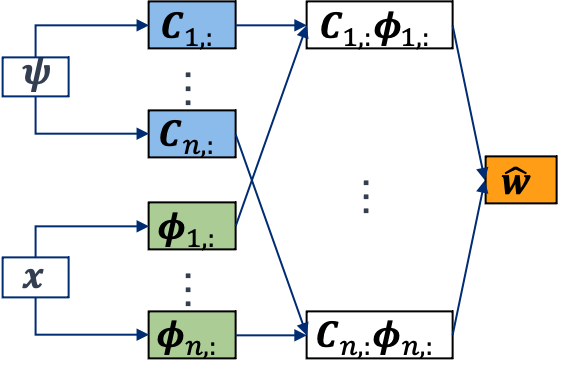
Figure 1: The NBF formulation ingests spatial points $\mathbf{x}$ and PDE parameters $\psi$ into separate sets of networks $\mathbf{\phi}$ and $\mathbf{C}$, and then the predicted state $\hat{\mathbf{w}}$ is a linear combination of these terms.

We consider the steady-state compressible Euler equations Certik (2017), defined for a state vector $\mathbf{w}_{\psi}=[\rho,u,v,E]^{T}$ on a domain $\Omega\subseteq R^{2}$:

$$\mathcal{S}_{\psi}\mathbf{w}_{\psi}:=\partial_{x}\mathbf{F}_{1}(\mathbf{w}_{\psi})+\partial_{y}\mathbf{F}_{2}(\mathbf{w}_{\psi})=0$$ (7)

where

$$\mathbf{F}_{1}=\begin{bmatrix}\rho u\\ \rho u^{2}+p\\ \rho vu\\ (E+p)u\end{bmatrix},\,\,\,\,\mathbf{F}_{2}=\begin{bmatrix}\rho v\\ \rho uv\\ \rho v^{2}+p\\ (E+p)v\end{bmatrix}.$$ (8)

The components of the state vector $\mathbf{w}_{\psi}$ include the fluid density $w_{0}=\rho$, the $x$ and $y$ velocities $w_{1}=u$ and $w_{2}=v$, and the total energy $w_{3}=E$.

The Euler equations Equation 7 also include the system pressure $P$, which is determined by a closure relation in terms of the other state variables:

$$P = (\gamma-1)[E-\frac{1}{2}\rho(u^{2}+v^{2})]$$

$$= (\gamma-1)[w_{3}-\frac{1}{2}w_{0}(w_{1}^{2}+w_{2}^{2})]$$

where $\gamma$ is the gas constant and is set to 1.4, using the perfect gas assumption.

Ultimately, we are interested in using solutions to these equations as initial conditions for a high fidelity CFD solvers to accelerate convergence. In additional term the state variable terms we will also need a relation for the temperature, $T$, which can be expressed as:

$$T=\frac{P}{R\rho}=\frac{P}{Rw_{0}}$$ (9)

where $R$ represents the ratio of specific heats and for this problem we set it to a constant $287.058$, also under the perfect gas assumption. The final term that will be referenced in this example is the speed of the flow and accounts for the magnitude of the $x$ and $y$ components of velocity ($|\mathbf{u}|=\sqrt{u^{2}+v^{2}}$). With these variables we can write the equation for the Mach number:

$$M=\frac{|\mathbf{u}|}{\sqrt{\gamma RT}}$$ (10)

which will be used in the inlet boundary condition described in Section 3.1. For further expansion of the Euler equations in terms of our state variables please see Appendix A.

2.4 Related work

The operator-learning problem is frequently viewed as learning mappings between function-spaces Lu et al. (2019a); Li et al. (2020); Bhattacharya et al. (2021), where the input function might be an initial condition or forcing function. We consider a more restricted setting, in that we require our operators $\mathcal{S}_{\phi}$ Equation 1 and $\mathcal{B}_{\psi}$ Equation 2 to be parametric functions of a finite-dimensional vector $\psi$. In both cases, however, the output is a function Equation 3 defined over an entire domain.

Of operator-learning approaches, the NBF is most similar to the DeepONet Lu et al. (2019a). Both use multiple types of networks that ingest different types of data (called “branch” and “trunk” networks in Lu et al. (2019a)). In particular, the NBF can be viewed as a extension of the recently-proposed POD DeepONet Lu et al. (2022). The POD DeepONet retains the full discrete set of bases Equation 6, but the NBF regresses these bases onto a set of neural networks $\phi_{i,j}$. This has a few benefits: It 1) can interpolate the modes to new regions of space when data are only available on sparse or unstructured grids; 2) is useful for lower memory applications where storing the potentially large full reduced basis is not feasible; and 3) allows for the ability to compute spatial and/or temporal derivatives of modeled quantities like fluid velocity in a batch process via GPU or another distributed architecture.

The NBF formulation, like the DeepONet formulation, does not impose any structure to the domain $\Omega$. This is in contrast to some methods like the Fourier Neural Operator Li et al. (2020). Our use case for the Euler equations in Section 3.1 relies on this flexibility. See also Lu et al. (2022) for a discussion of how different operator-learning approaches deal with non-uniform domains.

3 Results

3.1 Evaluation of NBF for Euler Equation

For this work, we will make use of a rectangular domain with a quarter circle cutout located at $x=[0,0]$ with radius 1 (see Figure 3). There is an inflow condition on the left side of the domain which is controlled by the Mach number, which for this study is the sole parameter in $\psi$. The domain extends to $-4$ in the $x$-direction and $7$ in the $y$-direction. This domain was chosen to allow sufficient room for the shock condition based on our predefined parametric Mach number range. This 2D cylinder in cross-flow problem is often used as a benchmark in the CFD space for testing different algorithms and their ability to capture shockwaves.

We then generated a steady-state dataset of high-fidelity solutions ranging from Mach 10 to Mach 30 in increments of 1. This data was generated using CFD++ in a time-dependent configuration and allowed to evolve until the time derivative portion of Euler equation sufficiently decreased. CFD++ is an unstructured finite volume flow solver that is maintained by Metacomp Technologies Inc. It has the capability of solving the full Navier-Stokes equations with high-order spatial and temporal accuracy. To resolve the inviscid Euler equations, the solver uses a pseudo time-marching approach where the initial condition is integrated over time until convergence is reached. The convergence can be accelerated by using spatially varying time steps. CFD++ version 20.1 was utilized to perform all the simulations.

Once we have the data generated, the next step is to extract the basis from the set of snapshots. In general, we hope to be able to approximate solutions within the parameter space, so, for analysis of this approach, we hold out a set of Mach cases as our test set. An ablation study of various number of training data points considered will be presented at the end of this section. But unless specifically noted, the results presented will use a dataset of 20 Mach numbers with just a single held-out solution. This is done to illustrate the best case scenarios for how well this approach applies.

Given the training data considered, we extract the state variables of interest and subtract the mean state from each of the solutions. Empirically, we have found that this tends to improve the speed of convergence when regressing the basis networks. The basis networks we consider are general fully-connected networks with five layers and 40 nodes per layer. We use leaky rectifed linear units Maas et al. (2013) as activation functions (with a negative slope of 0.01) on the hidden layers, which tends to help resolve the small-scale features in the basis functions. For example in Figure 2, the shock is very narrow in space and changes rather rapidly. We use the Adam optimizer Kingma & Ba (2015) and 250 total training epochs with an initial learning rate of $10^{-3}$ while applying an exponential learning rate decay factor (0.9) after 70 training epochs.

For PDEs with complicated phenomena (shockwaves), we have found accurately representing the high-frequency basis functions can be challenging. To resolve this, we use an importance sampling technique during training that prioritizes diverse data points in the training routine. We can describe the probability $p_{i,j,l}$ of selecting a single training data point when minimizing Equation 4, $(\mathbf{x}_{l}$, $U_{i,j}(\mathbf{x}_{l}))$, as:

$$p_{i,j,l}=\frac{p^{*}_{i,j,l}}{\sum_{l^{\prime}}p^{*}_{i,j,l^{\prime}}},$$ (11)

where $p^{*}_{i,j,l}=|U_{i,j}(\mathbf{x}_{l})-\bar{U}_{i,j}(\mathbf{x}_{l})|$, and $\bar{U}$ is the mean basis value for all spatial points in the domain $\mathbf{x}$. In practice, we have found that overusing this sampling approach leads to poor generalization. However, applying this methodology every so often (specifically every 4 epochs) improves the resolution of nuanced features.

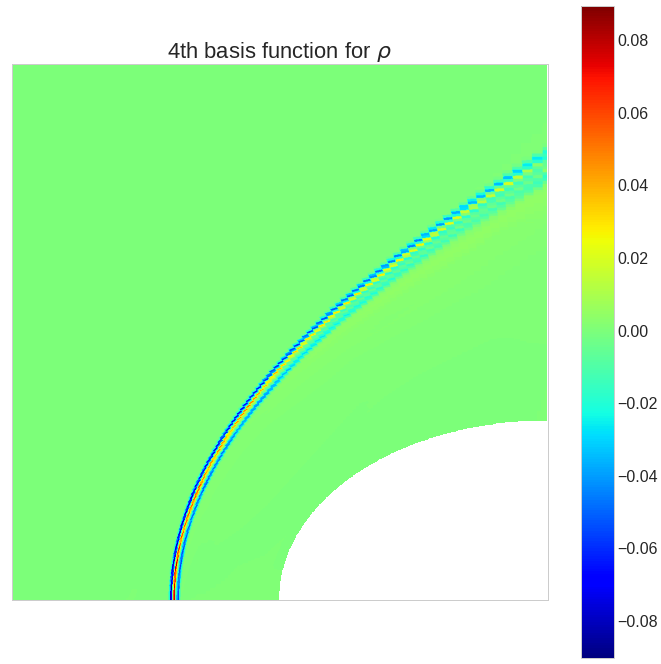
Figure 2: To demonstrate the complex spatial features inherent in higher-frequency basis functions, we visualize the predicted fourth basis for the density $\rho$ as a function of spatial coordinates $\mathbf{x}$. This is a zoomed in version around the shock region.

Once the basis networks have been sufficiently trained, the next step is to learn the set of unknown networks. For unknown network configurations, we use a seven layer feed forward network with 120 nodes per layer with leaky ReLU activation functions, similar to the basis networks. In practice, we have found that Equation 5 is non-trivial to learn with standard weight initialization techniques. To aid convergence of this loss term, we use a pre-training approach that attempts to regress the $C_{i,j}$ terms to known solution data to get the unknown network weights in a sufficient neighborhood before applying the operator loss in Equation 5. This pre-training minimization loss can be written as:

$$\min_{\tilde{C}_{i,j}}\sum_{\psi}\sum_{l}|C_{i,j}(\mathbf{x}_{l},\psi)-\tilde{C}_{i,j}(\mathbf{x}_{l},\psi)|^{2},$$ (12)

where $\tilde{C}_{i,j}$ can be calculated through standard minimization according to the loss function:

$$\min_{\tilde{C}_{i,j}}\sum_{\psi}\sum_{l}\left|\sum_{j}\tilde{C}_{i,j}(\mathbf{x}_{l},\psi)\phi(\mathbf{x}_{l})-\mathbf{w}(\mathbf{x}_{l},\psi)\right|^{2}$$ (13)

this allows the unknown network to start off with a reasonable estimate of the desired states. It is important to note that, during this learning process, we place no dependencies on the operator portion, $\mathcal{S}_{\psi}\hat{\mathbf{w}}(\mathbf{x},\psi)$, in the loss function.

After pre-training, the final step is to optimize the unknown network with respect to the governing equations, boundary conditions and any other constraints. Minimization of the governing equations and boundary conditions follows the definition of the Euler equations and the loss function defined in Equation 5. For this problem we add two additional constraints to minimize the mean square error between predicted and CFD Pressures and Temperatures. Unfortunately incorporating this constraint restricts our loss function to only use $\psi$ parameters that exist in our training set. However, we have found that without incorporating this constraint leads to negative values of pressure/temperature which for this problem are non-physical.

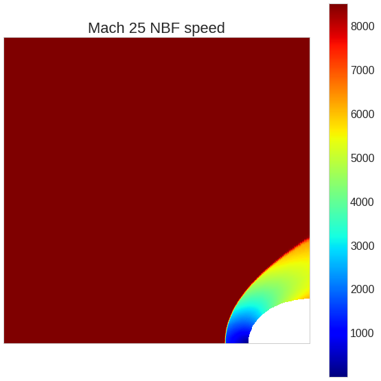
Figure 3: The predicted NBF approximation of speed $\sqrt{u^{2}+v^{2}}$ at the test point, Mach 25. The majority of the domain (solid color) has high values of speed, then, at the shockwave (bottom right), the speed distribution rapidly changes.

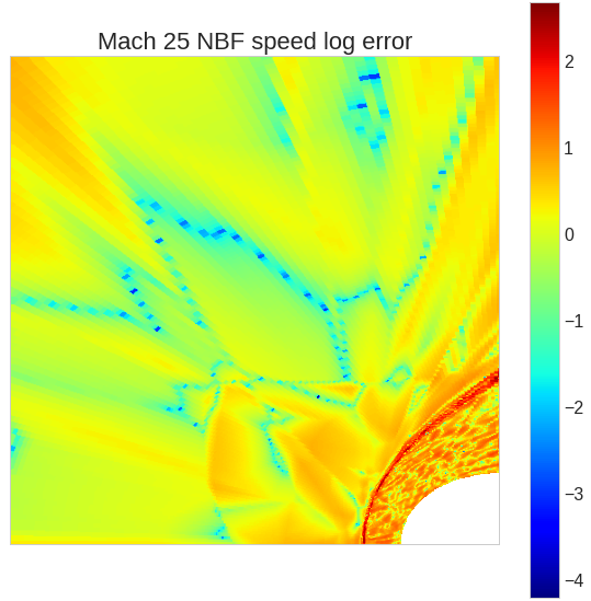
Figure 4: We evaluate our NBF prediction of speed for the Mach 25 test case with the log absolute error compared to the ground truth. The errors are highest near the boundary of the shockwave.

Finally with the basis and unknown networks trained, we are able to infer new solutions within the defined parameter space. We seek to generalize performance across the parameter space $\Psi$ of Mach numbers. Figure 3 shows the NBF predicted solution for the speed within the domain while considering a Mach 25 inflow condition. Figure 4 shows the log absolute error of this predicted solution with respect to the CFD++ data. It is worth noting that this particular scenario is held out of our training data set and still shows good predictive performance.

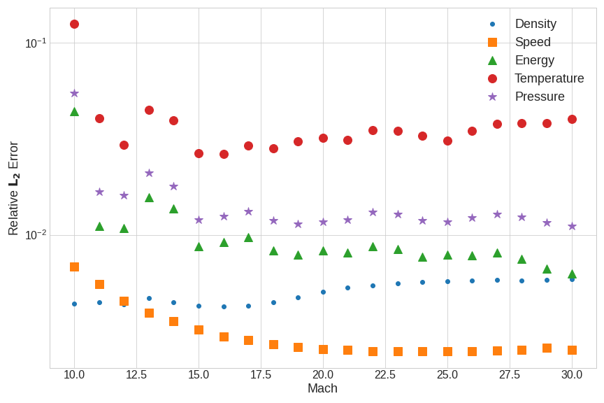
Figure 5: Relative $L_{2}$ error for variables of interest with respect to Mach number, for the test data (Mach 25) and training data (remainder).

It is also useful to understand how well the NBF approximation works across the parameter space. Figure 5 shows the relative $L_{2}$ error as a function of the Mach number. The errors appear to be relatively stable across the parameter space with slightly better performance for the higher Mach numbers.

3.2 Comparison with Vanilla DeepONet

In order to understand how well the NBF approach compares against existing approaches, we will benchmark our solution against the Vanilla DeepONet operator approach. The equation for the vanilla DeepONet is given by Lu et al. (2022):

$$\mathcal{G}(v)(\xi)=\sum_{j=1}^{q}b_{j}(v)t_{j}(\xi)+b_{0}$$ (14)

where $v$ and $\xi$ are the parameter (in our case $\psi$) and spatial values (in our case $\mathbf{x}$). Lu et al. (2022) focuses on the case where $v$ is a function that parameterizes the PDE – for example, an initial condition. For comparison purposes, we will consider it a parameterization of $\Psi$. Additionally, $b_{j}(v)$ and $t_{j}(\xi)$ represent the branch and trunk networks respectively, with $b_{0}$ acting as a bias imposed on the outputs.

Since we are interested in the two dimensional steady state Euler equations, we require a DeepONet representation of multiple state variables defined in  Equation 8. Making use of recommendations from Lu et al. (2022), we implement a set of feed-forward DeepONets for each state variable considered. The network architectures that we found generated the best performance for our use case comprised of: 5 layers of 120 nodes with hyperbolic tangent activation functions for the branch networks and 6 layers of 120 nodes with rectified linear units for the trunk networks. These networks were then connected in a shared layer of 64 nodes combined with a bias ($b_{0}$) to produce predictions for each state variable. During training, we used the same Adam optimizer, learning rate decay and number of epochs as was used for the NBF approach.

We added a few components that appeared to aid the training process for our problem specifically: adding prioritized spatial sampling and zero-mean unit-variance (ZMUV) normalization functions for spatial/parameter inputs as well as the output state variables. For spatial sampling prioritization we used the Equation 11 to more often select training examples with more deviation from the mean solution. Additionally, adding the ZMUV normalization to input/output parameters appeared to speed convergence and prevent collapsing the solution to the mean flow.

Figure 6 shows the comparison for the vanilla DeepONet vs the Neural Basis Function approach considering the total number of training solutions as inputs. We are able to show better performance in the approximation across the number of training examples. Specifically we are able to produce significantly better results for smaller training data sets, indicating better generalization for sparse data. We believe we are able to show this better performance due to the pre-conditioned nature of basis functions included in the NBF estimates as well as application of the governing equation as regularization during training.

It is worth noting, that although the training process lines up reasonably closely between the two approaches, there is some overhead incurred by the NBF approach in: calculating the SVD, then training the unknown network. Additionally, the DeepONet architecture is significantly smaller than the NBF architecture as it is described here. We believe there are architecture optimizations that could reduce the size and will consider this for future work. Thus, it is not a completely direct comparison but is as close as we could get to provide a baseline for the NBF approach.

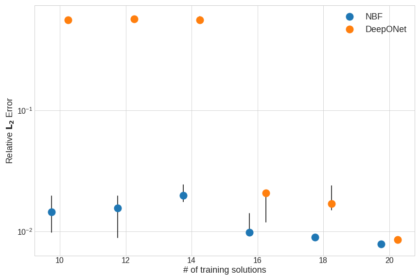
Figure 6: As an ablation study, we vary the amount of training data and evaluate $L_{2}$ relative error for the test set. The dots represent the median error with the black tails indicating inner 50th percentile. Blue show NBF relative error compared to the orange of the vanilla DeepONet

We found that for many of the cases within the ablation study, the Energy ($E$) state variable was the most difficult to get to converge. This is likely due to the magnitude of values compared to the other state variables ($\rho$, $u$ and $v$). For DeepONet, applying the ZMUV transformation on the output state improved the convergence but not significantly so.

3.3 Acceleration of CFD solutions

In the conventional CFD approach an initial condition is employed with iterative updates until steady state is reached. If one was to use an initial condition that is close to the converged solution, fewer iterations would be required to reach the high-fidelity steady-state. The NBF solution can be leveraged to accelerate the CFD solver by providing this nearly converged initial condition. In the following section, we will compare the performance of the conventional CFD approach with NBF informed CFD approach. The two approaches will be evaluated by comparing their average residual history. The time-dependent form of the Euler equation includes the the term:

$$\frac{\partial\mathbf{w}}{\partial t}$$ (15)

and adds to Equation 8. Additional details on the setup and implementation of the CFD++ configuration can be found in Appendix C

The convergence is determined by the evolution of the time-dependent residual. Once the residual levels off, the simulation is deemed to be converged and the solution has reached steady-state. In the CFD++ finite volume approach, the governing equations are integrated over the cell volumes. For the case of the Euler equations, the right hand side becomes the sum of the scalar product of the inviscid fluxes and the cell face areas. For a given equation, the residual is defined as the absolute value of the residual divided by the cell volume averaged over all the cells. Since we are working with a system of equations, we monitor the average residual of our system equations, i.e. the sum of the residual of each equation divided by the number of equations. Additional detail of all the numerical procedures can be found in the CFD++ user-manual.

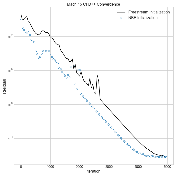
Figure 7: Steady state convergence acceleration of a Mach 15 scenario. Using the NBF prediction as the initialization results in a speedup of roughly 750 iterations compared to the freestream initialization.

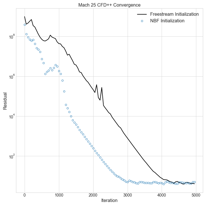
Figure 8: Steady state convergence acceleration of a Mach 25 scenario. Using the NBF prediction as the initialization results in a speedup of roughly 1000 iterations, compared to the freestream initialization.

Figure 7 and Figure 8 show the time-dependent residual as a function of the number of iterations for Mach 15 and 25 respectively. As we can see from these plots, the NBF solution provides a noticeable speed up in the convergence of the high fidelity solver.

4 Discussion

This work has shown the potential for using an operator learning based approach, like the Neural Basis Function, as an acceleration mechanism for high-fidelity CFD solvers. We found that regressing a set of networks to POD basis data, then using an additional unknown network in linear combination can provide sufficient estimates of state variables within a configurable parameter space. High Mach flow cases often induce complicated phenomena, like discontinuous shockwaves, which are difficult to represent numerically, even with standard techniques. Using the 2D steady state Euler equations as an example, we were able to produce accurate estimates to the flow field for high Mach (10-30) scenarios. These solutions were then used as initial conditions to a high-fidelity CFD solver (CFD++) to improve the convergence, resulting in speed ups up to 1000 iterations.

As future work on the application side, we intend to extend these results to the full Navier-Stokes equations, while transitioning to a three-dimensional domain. Along the way improvements will be made to the methodology to better understand network architecture performance as well as improving training techniques for the basis and unknown networks. We also hope to develop a methodology using NBF (or other operator approaches) to handle problems where the spatial domain might vary across snapshots. This would allow for the ability to do shape optimization or analysis of multiple geometric configurations.

On the learning side, we hope to factor in an active learning feedback loop Settles (2009) that will be able to identify regions of the $\psi$ parameter space with poor predictive performance, in order to execute more high-fidelity scenarios in these regions to improve overall accuracy. Finally, some combination of DeepOnet and NBF seems like a reasonable path forward especially for speeding convergence of these techniques. For example, one could create a set of trunk networks that are regressed from the orthogonal SVD basis, then freeze their weights and biases. Then adding a vanilla DeepONet in combination with these bases could greatly speed the convergence and make it easier to implement an active learning type of approach for data generation.

Appendix A Euler Equation Expansion

We can expand the Euler equations in terms of our state variables $\mathbf{w}$:

$$\mathbf{F}_{1} = [f_{11},f_{12},f_{13},f_{14}]^{T}$$

$$f_{11} = \rho u$$

$$= w_{0}w_{1}$$

$$f_{12} = \rho u^{2}+p$$

$$= w_{0}w_{1}^{2}+(\gamma-1)[w_{3}-\frac{1}{2}w_{0}(w_{1}^{2}+w_{2}^{2})]$$

$$f_{13} = \rho uv$$

$$= w_{0}w_{1}w_{2}$$

$$f_{14} = (E+p)u$$

$$= (w_{3}+(\gamma-1)[w_{3}-\frac{1}{2}w_{0}(w_{1}^{2}+w_{2}^{2})])w_{1}$$

$$\mathbf{F}_{2} = [f_{21},f_{22},f_{23},f_{24}]^{T}$$

$$f_{21} = \rho v$$

$$= w_{0}w_{2}$$

$$f_{22} = \rho uv$$

$$= w_{0}w_{1}w_{2}$$

$$f_{23} = \rho v^{2}+p$$

$$= w_{0}w_{2}^{2}+(\gamma-1)[w_{3}-\frac{1}{2}w_{0}(w_{1}^{2}+w_{2}^{2})]$$

$$f_{24} = (E+p)v$$

$$= (w_{3}+(\gamma-1)[w_{3}-\frac{1}{2}w_{0}(w_{1}^{2}+w_{2}^{2})])w_{2}$$

Appendix B Other Variable Field Visuals

The following set of plots provide a visual for the other variables of interest using the NBF approximation to the Mach 25 scenario.

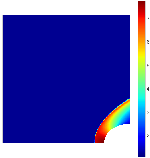
Figure 9: Density ($\rho$)

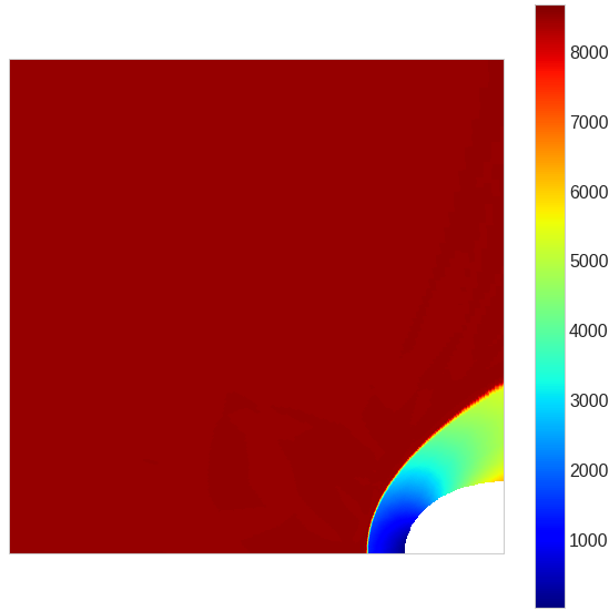
Figure 10: $x$-velocity component ($u$)

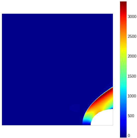
Figure 11: $y$-velocity component ($v$)

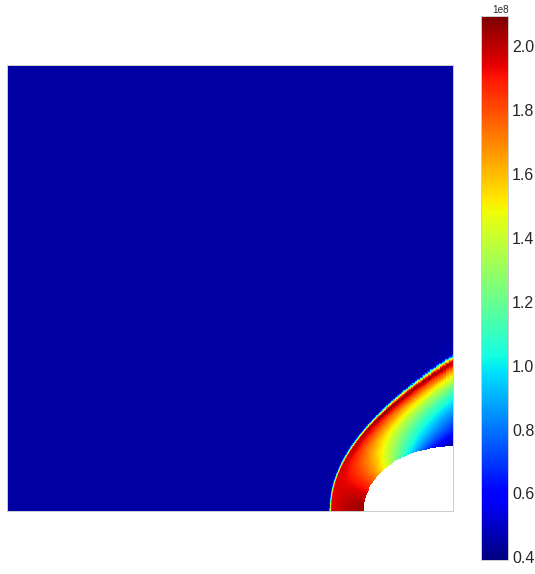
Figure 12: Energy ($E$)

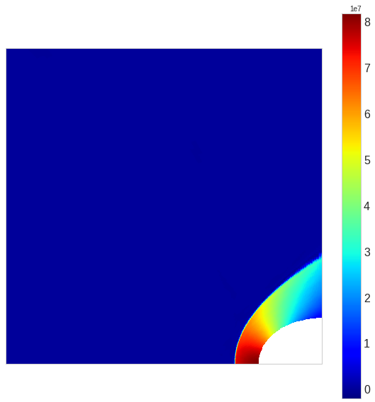
Figure 13: Pressure ($P$)

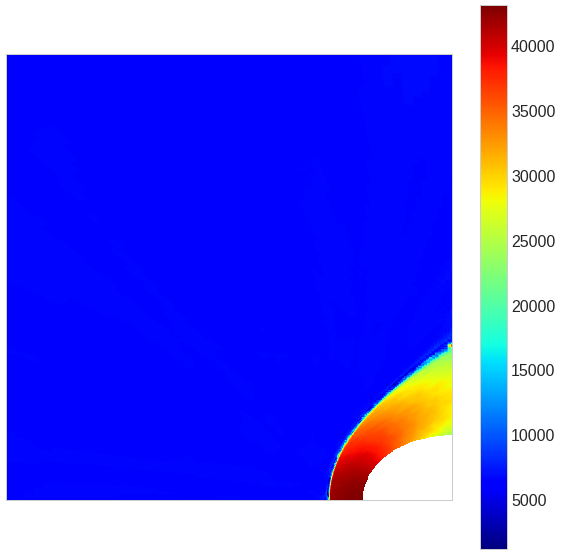
Figure 14: Temperature ($T$)

Appendix C CFD++ Details

In our investigation, CFD++ was run with a second order spatial discretization scheme. The inviscid fluxes were calculated based on the minmod TVD limiter. The fluxes on the cell faces were reconstructed based on centroidal polynomials. Spatial scheme blending was leveraged for the sake of numerical stability. During the initial 250 iterations, first order fluxes were used exclusively. Then a linear blending of the first and second order discretization scheme was used until iteration 750, beyond which the second order fluxes were used exclusively.

The time-residual from iteration to iteration depends on the integration scheme. In this study, an implicit Gauss-Seidel relaxation time integration scheme was utilized with no additional convergence acceleration methods. The time step sizes were based on the local (spatially varying) CFL (Courant Friedrichs-Lewy) number. The CFL number is a dimensionless number that is equal to the time step size scaled by the time it takes for the fasts moving characteristics to travel across a cell $CFL=\frac{dt}{\frac{dx}{|\mathbf{u}|+a}}$, recalling $|\mathbf{u}|$ is the scaler speed field. $a$ is the speed of sound ($a=\sqrt{T*R*\gamma}$) In each simulations, the CFL number was linearly increased from 0.01 to 10 over the first 1000 iterations beyond which the CFL number was kept constant.

References

- Baydin et al. (2017) Baydin, A. G., Pearlmutter, B. A., Radul, A. A., and Siskind, J. M. Automatic differentiation in machine learning: A survey. J. Mach. Learn. Res., 18(1):5595–5637, jan 2017. ISSN 1532-4435.
- Berkooz et al. (1993) Berkooz, G., Holmes, P., and Lumley, J. L. The proper orthogonal decomposition in the analysis of turbulent flows. Annual review of fluid mechanics, 25(1):539–575, 1993.
- Bhattacharya et al. (2021) Bhattacharya, K., Hosseini, B., Kovachki, N. B., and Stuart, A. M. Model Reduction And Neural Networks For Parametric PDEs. The SMAI journal of computational mathematics, 7:121–157, 2021. doi: 10.5802/smai-jcm.74.
- Certik (2017) Certik, O. Theoretical physics reference. 2017.
- Gunzburger et al. (2007) Gunzburger, M. D., Peterson, J. S., and Shadid, J. N. Reduced-order modeling of time-dependent pdes with multiple parameters in the boundary data. Computer methods in applied mechanics and engineering, 196(4-6):1030–1047, 2007.
- Han et al. (2018) Han, J., Jentzen, A., and E, W. Solving high-dimensional partial differential equations using deep learning. Proceedings of the National Academy of Sciences, 115(34):8505–8510, 2018. ISSN 0027-8424. doi: 10.1073/pnas.1718942115.
- He & Zou (2021) He, H. and Zou, R. functorch: Jax-like composable function transforms for pytorch. https://github.com/pytorch/functorch, 2021.
- Karniadakis et al. (2021) Karniadakis, G. E., Kevrekidis, I. G., Lu, L., Perdikaris, P., Wang, S., and Yang, L. Physics-informed machine learning. Nature Reviews Physics, 3(6):422–440, 2021.
- Kashinath et al. (2021) Kashinath, K., Mustafa, M., Albert, A., Wu, J.-L., Jiang, C., et al. Physics-informed machine learning: case studies for weather and climate modelling. Philosophical Transactions of the Royal Society A: Mathematical, Physical and Engineering Sciences, 379(2194):20200093, 2021. doi: 10.1098/rsta.2020.0093.
- Khan & Lowther (2022) Khan, A. and Lowther, D. A. Physics informed neural networks for electromagnetic analysis. IEEE Transactions on Magnetics, pp. 1–1, 2022. doi: 10.1109/TMAG.2022.3161814.
- Kingma & Ba (2015) Kingma, D. P. and Ba, J. Adam: A method for stochastic optimization. In Bengio, Y. and LeCun, Y. (eds.), 3rd International Conference on Learning Representations, ICLR 2015, San Diego, CA, USA, May 7-9, 2015, Conference Track Proceedings, 2015.
- Li et al. (2020) Li, Z., Kovachki, N., Azizzadenesheli, K., Liu, B., Bhattacharya, K., Stuart, A., and Anandkumar, A. Fourier neural operator for parametric partial differential equations. arXiv preprint arXiv:2010.08895, 2020.
- Lu et al. (2019a) Lu, L., Jin, P., and Karniadakis, G. E. Deeponet: Learning nonlinear operators for identifying differential equations based on the universal approximation theorem of operators. arXiv preprint arXiv:1910.03193, 2019a.
- Lu et al. (2019b) Lu, L., Meng, X., Mao, Z., and Karniadakis, G. E. Deepxde: A deep learning library for solving differential equations. CoRR, abs/1907.04502, 2019b.
- Lu et al. (2022) Lu, L., Meng, X., Cai, S., Mao, Z., Goswami, S., Zhang, Z., and Karniadakis, G. E. A comprehensive and fair comparison of two neural operators (with practical extensions) based on fair data. Computer Methods in Applied Mechanics and Engineering, 393:114778, 2022.
- Maas et al. (2013) Maas, A. L., Hannun, A. Y., and Ng, A. Y. Rectifier nonlinearities improve neural network acoustic models. In in ICML Workshop on Deep Learning for Audio, Speech and Language Processing, 2013.
- Mao et al. (2020) Mao, Z., Jagtap, A. D., and Karniadakis, G. E. Physics-informed neural networks for high-speed flows. Computer Methods in Applied Mechanics and Engineering, 360:112789, 2020. ISSN 0045-7825. doi: https://doi.org/10.1016/j.cma.2019.112789.
- Mao et al. (2021) Mao, Z., Lu, L., Marxen, O., Zaki, T. A., and Karniadakis, G. E. Deepm&mnet for hypersonics: Predicting the coupled flow and finite-rate chemistry behind a normal shock using neural-network approximation of operators. Journal of Computational Physics, 447:110698, 2021. ISSN 0021-9991. doi: https://doi.org/10.1016/j.jcp.2021.110698.
- Paszke et al. (2019) Paszke, A., Gross, S., Massa, F., Lerer, A., Bradbury, J., et al. Pytorch: An imperative style, high-performance deep learning library. In Wallach, H., Larochelle, H., Beygelzimer, A., d'Alché-Buc, F., Fox, E., and Garnett, R. (eds.), Advances in Neural Information Processing Systems 32, pp. 8024–8035. Curran Associates, Inc., 2019.
- Quarteroni et al. (2015) Quarteroni, A., Manzoni, A., and Negri, F. Reduced basis methods for partial differential equations: an introduction, volume 92. Springer, 2015.
- Raissi et al. (2019) Raissi, M., Perdikaris, P., and Karniadakis, G. E. Physics-informed neural networks: A deep learning framework for solving forward and inverse problems involving nonlinear partial differential equations. Journal of Computational Physics, 378:686–707, 2019.
- Settles (2009) Settles, B. Active learning literature survey. 2009.
- Sirovich (1987) Sirovich, L. Turbulence and the dynamics of coherent structures. i. coherent structures. Quarterly of applied mathematics, 45(3):561–571, 1987.
- Willard et al. (2020) Willard, J., Jia, X., Xu, S., Steinbach, M., and Kumar, V. Integrating scientific knowledge with machine learning for engineering and environmental systems, 2020. URL https://arxiv.org/abs/2003.04919.
- Willcox & Peraire (2002) Willcox, K. and Peraire, J. Balanced model reduction via the proper orthogonal decomposition. AIAA journal, 40(11):2323–2330, 2002.
- Witman et al. (2017) Witman, D. R., Gunzburger, M., and Peterson, J. Reduced-order modeling for nonlocal diffusion problems. International Journal for Numerical Methods in Fluids, 83(3):307–327, 2017.
- Yazdani et al. (2021) Yazdani, A., Deng, Y., Li, H., Javadi, E., Li, Z., Jamali, S., Lin, C., Humphrey, J. D., Mantzoros, C. S., and Em Karniadakis, G. Integrating blood cell mechanics, platelet adhesive dynamics and coagulation cascade for modelling thrombus formation in normal and diabetic blood. Journal of The Royal Society Interface, 18(175):20200834, 2021. doi: 10.1098/rsif.2020.0834.