Dust, CO and [C i]: Cross-calibration of molecular gas mass tracers in metal-rich galaxies across cosmic time

Abstract

We present a self-consistent cross-calibration of the three main molecular gas mass tracers in galaxies, namely the ¹²CO(1–0), [C i](${}^{3}P_{1}$–${}^{3}P_{0}$) lines, and the submm dust continuum emission, using a sample of 407 galaxies, ranging from local disks to submillimetre-selected galaxies (SMGs) up to $z\approx 6$. A Bayesian statistical method is used to produce galaxy-scale universal calibrations of these molecular gas indicators, that hold over 3–4 orders of magnitude in infrared luminosity, $L_{\rm IR}$. Regarding the dust continuum, we use a mass-weighted dust temperature, $T_{\rm mw}$, determined using new empirical relations between temperature and luminosity. We find the average L/$M_{\rm mol}$ gas mass conversion factors (including He) to be $\mbox{$\alpha_{850}$}=6.9\times 10^{12}\,\rm W\,Hz^{-1}\,M_{\odot}^{-1}$, $\alpha_{\rm CO}$=4.0 M_⊙ (k km s^-1 pc²)^-1 and $\alpha_{\rm C\,I}$=17.0 M_⊙ (k km s^-1 pc²)^-1, based on the assumption that the mean dust properties of the sample ($\kappa_{\rm H}$= gas-to-dust ratio/dust emissivity) will be similar to those of local metal rich galaxies and the Milky Way. The tracer with the least intrinsic scatter is [C i](1–0), while CO(1–0) has the highest. The conversion factors show a weak but significant correlation with $L_{\rm IR}$ which is not apparent when $T_{\rm mw}$ is held constant. Assuming dust properties typical of metal-rich galaxies, we infer a neutral carbon abundance $\mbox{$X_{\rm C\,I}$}=\rm[C^{0}/\mbox{H${}_{2}$}]=1.6\times 10^{-5}$, similar to that in the Milky Way. We find no evidence for bi-modality of $\alpha_{\rm CO}$ between main-sequence (MS) galaxies and those with extreme star-formation intensity, i.e. ultraluminous infrared galaxies (ULIRGs) and SMGs. The means of the three conversion factors are found to be similar between MS galaxies and ULIRGs/SMGs, to within 10–20 per cent. The overarching conclusion of our work is that, for metal-rich galaxies, near-universal average values for $\alpha_{\rm CO}$, $X_{\rm C\,I}$ and $\kappa_{\rm H}$ are adequate for global molecular gas estimates within the expected uncertainties. The 1$\sigma$ scatter in our optimised values for $\alpha_{\rm CO}$, $X_{\rm C\,I}$ and $\kappa_{\rm H}$ are 0.14, 0.11 and 0.15 dex respectively.

1 Introduction

The cosmic star-formation rate (SFR) density has declined by more than an order of magnitude during the past $\approx 8$ Gyr of cosmic history (Lilly et al., 1996; Madau et al., 1996; Madau & Dickinson, 2014). The driver of star formation is the molecular gas supply in galaxies, and indeed the SFR–stellar mass (SFR–$M_{\star}$) relationship known as the galaxy main sequence (MS) is purely a by-product of the relationship between SFR and molecular gas (e.g. Baker et al., 2022), for unperturbed galaxies with significant gas reserves. A major observational goal is to produce a combined census of the molecular gas – the ‘potential for future star formation’ – and the stellar content – the ‘record of past star formation’ – over this period (e.g. Keres et al., 2003; Dunne et al., 2003; Dunne et al., 2011; Zwaan et al., 2004; Zafar et al., 2013; Walter et al., 2014; Decarli et al., 2016; Saintonge et al., 2017; Driver et al., 2018; Rhee et al., 2018; Decarli et al., 2019; Riechers et al., 2019).

The molecular gas fraction of a galaxy is a crucial component in models of galaxy formation (e.g. Obreschkow et al., 2009; Popping et al., 2014; Lagos et al., 2015; Chen et al., 2018) and thus measurements of $\rm H_{2}$ and stellar mass over large representative galaxy samples are key requirements for understanding how galaxies have transformed from clouds of gas residing in dark matter haloes into the regular agglomerations of stars we see in the local Universe. While it is clear that CO(1–0)-luminous gas is the phase linked with star formation (e.g. Wong & Blitz, 2002), observations of molecules with higher critical densities (e.g. HCN) revealed that it is the dense H₂ gas phase ($n>10^{4}$ cm^-3) that correlates most tightly and linearly with tracers of star-formation (Gao & Solomon, 2004).

Atomic hydrogen (H i), on the other hand, constitutes a longer-term gas reservoir for star formation, where under certain conditions of pressure, far-UV radiation field, density and metallicity, a phase transition H i $\rightarrow$ H₂ takes place, catalysed by dust grains (e.g. Elmegreen, 1993; Papadopoulos et al., 2002; Blitz & Rosolowsky, 2006): a picture supported by numerous observations (e.g. Honma et al., 1995; Leroy et al., 2008; Bigiel et al., 2008; Schruba et al., 2011). This transition occurs in the inner H i distribution of galaxies, in the cold neutral medium (CNM: $n\sim 50$–100 cm^-3, $T_{\rm kin}\sim 100$–200 k), meanwhile pure H i gas often extends many optical radii beyond the luminous stellar disk (e.g. Péroux & Howk, 2020), where it can be found concomitant with cold dust (e.g. Thomas et al., 2002).

Unlike H i  and its hyperfine line emission at 21 cm, the H₂ molecule in its S(0):$J=2-0$ transition at 28$\mu$m (the least excitation-demanding $\rm H_{2}$ line) is essentially invisible at temperatures typical of giant molecular clouds (10–20 k). This is because its $\Delta E/k_{\rm B}$$\sim$$510\,{\sc k}$, limits its excitation and detetection only to shocked regions of molecular clouds, where gas temperatures can rise past $\sim 1000$ k, for small ($\sim 1$–2 per cent) gas mass fractions. Even then, to observe this H₂ line at 28 $\mu$m requires space-borne telescopes.

For these reasons the rotational transitions of CO (the next most abundant molecule with $\rm[CO/H_{2}]\sim 10^{-4}$) are commonly used to trace $\rm H_{2}$ gas, with the lowest transition (¹²CO $J=1$–0) being the most established tracer. Its $E_{10}/k_{\rm B}\sim 5.5$ k ensures a well-populated upper level even in the coldest gas, while its low critical density, $n_{\rm cr}\sim 400$ cm^-3, ensures its excitation even at low densities.

The CO(1–0) line has significant optical depths in the typically macro-turbulent $\rm H_{2}$ gas, though these arise locally within the velocity-coherent gas cells allowing the CO emission to trace gas mass throughout molecular clouds (e.g. Dickman et al., 1986). The conversion factor, $\alpha_{\rm CO}$, in the relation $\mbox{$M_{\rm H2}$}=\mbox{$\alpha_{\rm CO}$}\mbox{$L^{\prime}_{\rm CO}$}$ cannot be determined using standard optically thin line formation physics due to the high line optical depths. This created the need for a $\alpha_{\rm CO}$ calibration as soon as the ubiquity of CO line emission in H₂ clouds was established. Observational and theoretical investigation of $\alpha_{\rm CO}$ suggests it is sensitive to metallicity, molecular gas surface density and kinematic state in galaxies (e.g. Pelupessy & Papadopoulos, 2009; Narayanan et al., 2011; Papadopoulos et al., 2012a; Bolatto et al., 2013).

Three distinct problems are now recognised regarding the use of CO as a global tracer of H₂ mass in galaxies:

1. The $\alpha_{\rm CO}$ factor is sensitive – in a highly non-linear fashion – to the ISM metallicity and ambient far-UV radiation fields (e.g. Israel, 1997; Pak et al., 1998; Bolatto et al., 2013).

2. Non-self-gravitating molecular clouds – and/or very different average ISM states in terms of average temperature and gas density range from those found in spiral galaxies where $\alpha_{\rm CO}$ was first calibrated – can yield systematically different $\alpha_{\rm CO}$ factors. For example, $\alpha_{\rm CO}$$\sim 1/5-1/4\times$ Galactic was initially reported for a sample of four ULIRGs by Downes & Solomon (1998).

3. Elevated cosmic ray (CR) energy densities can destroy CO below a certain gas density threshold, leaving behind more C-rich gas. This density threshold depends on the CR energy density in a highly non-linear fashion, as explored by Bisbas et al. (2015), who found that regions of CO suppression may occur even in moderately enhanced CR conditions if the gas density is low, while the very high CR energy densities expected in ultraluminous infrared galaxies (ULIRGs) may be partly compensated by higher gas densities in such starbursts. Modelling [C i/CO] ratios as a function of CR, turbulence, gas density and metallicity is an active area of theoretical research (e.g. Bisbas et al., 2015; Bisbas et al., 2017; Bisbas et al., 2021; Glover & Clark, 2016; Clark et al., 2019a; Papadopoulos et al., 2018; Gong et al., 2020).

In the distant Universe, additional problems arise. High-redshift galaxies are often observed solely in high-$J$ CO lines ($J=3$–2 and higher), due to the observational challenge of observing the two low-$J$ CO lines. Using the high-$J$ lines means that global CO($J+1,J$)/(1–0) ratios must be assumed before an $\alpha_{\rm CO}$  factor can be used; given the wide range of CO spectral-line energy distributions (SLEDs) found for LIRGs for $J=3$–2 and higher (Papadopoulos et al., 2012b; Greve et al., 2014; Kamenetzky et al., 2016), these assumptions come with large uncertainties. Finally, at the highest redshifts ($\ga$4), low-$J$ CO lines (and dust emission) can be severely suppressed for cold gas (and dust) reservoirs due to their low contrast against the ambient, rest-frame cosmic microwave background (da Cunha et al., 2013; Zhang et al., 2016).

In principle, radiative transfer models of well-sampled CO (and ¹³CO) SLEDs can yield $\alpha_{\rm CO}$ values appropriate for a particular galaxy (or even galaxy class) (e.g. Papadopoulos et al., 2012b; Papadopoulos et al., 2014; Harrington et al., 2021). Nevertheless, the size of the CO line datasets per galaxy required to do this make it impractical (in terms of telescope time) to obtain $M$(H₂) for large galaxy samples. Amassing a large sample typically means only one or two lines can be gathered per galaxy, and thus a calibration of $\alpha_{\rm CO}$  and its uncertainties remains very valuable. The only practical way to achieve this is to cross-calibrate against the other galaxy-scale $\rm H_{2}$ mass tracers.

Large-area far-infrared (FIR) and submillimetre (submm) surveys (e.g. Armus et al., 2009; Eales et al., 2010; Vieira et al., 2010; Kennicutt et al., 2011; Oliver et al., 2012; Hodge et al., 2013) ushered in a new era in which submm continuum emission from dust has been used widely as an alternative tracer of $M_{\rm H2}$, although it has been clear that submm-derived dust masses ($\propto\mbox{$L_{850}$}$) and CO-derived molecular gas masses ($\propto\mbox{$L^{\prime}_{\rm CO}$}$) are tightly correlated ever since the first statistical submm survey of 100 local FIR-bright galaxies (SLUGS – Dunne et al., 2000). The first suggestions to use dust as an alternative to CO at high redshift (e.g. Santini et al., 2010; Magdis et al., 2012; Scoville et al., 2014) were followed quickly by work demonstrating its potential (e.g Scoville et al., 2016; Hughes et al., 2017; Orellana et al., 2017).

An advantage of using submm continuum emission from dust as an $\rm H_{2}$ gas tracer is that it becomes easier to measure at high redshift, because of the negative $K$-correction (e.g. Blain & Longair, 1993), while recent technological advances made it possible to image areas large enough to be free of cosmic variance, leading to the FIR/submm detection of many thousands of galaxies by the Herschel Space Observatory, for example. The use of dust as a gas mass proxy requires an estimate of metallicity, since the dust-to-gas ratio, $\delta_{\rm GDR}$, is roughly proportional to metallicity (e.g. Muñoz-Mateos et al., 2009; Magdis et al., 2012; Sandstrom et al., 2013; Draine et al., 2014). The appropriate $\delta_{\rm GDR}$  can then be applied (e.g. Valentino et al., 2018). Whilst this requirement is often raised as a problem regarding the use of dust as a gas mass tracer, its dependence on metallicity is in fact weaker than that of CO.

For galaxies selected at FIR/submm/mm wavelengths, it is safe to assume that the metallicity will be high, such that $\delta_{\rm GDR}$  will be broadly similar to those found for local metal-rich spirals and the Milky Way (Dunne & Eales, 2001; Draine, 2009; Magdis et al., 2012; Sandstrom et al., 2013; Rowlands et al., 2014; Yang et al., 2017; Berta et al., 2021). A detailed discussion of the advantages and disadvantages of using dust as a tracer of gas can be found in Genzel et al. (2015) and Scoville et al. (2017).

A third method of tracing molecular gas – the use of atomic carbon lines – has come to the fore since ALMA became operational. Its promise was recognised by Papadopoulos et al. (2004) and its first application as a tracer for molecular gas mass in galaxies gave good results (Weiß et al., 2003; Papadopoulos & Greve, 2004), implying that: a) the [C i](${}^{3}P_{1}$–${}^{3}P_{0}$) lines are optically thin for the bulk of $\rm H_{2}$ gas (Pérez-Beaupuits et al., 2015) and b) atomic carbon is present throughout CO-rich molecular cloud volumes.

The latter contradicts the earlier simple plane-parallel PDR model where atomic carbon (and its line emission) occupied only a thin layer, sandwiched between $\rm C^{+}$ in the outer and CO in the inner regions of FUV-illuminated molecular clouds (Tielens & Hollenbach, 1985). However observations have repeatedly shown excellent concomitance of C i line emission with CO line emission, by area and by velocity, and C i shows a tighter correlation with ¹³CO than with ¹²CO. C i  is now thought to arise from same volume as the CO, with similar excitation conditions (e.g. Plume et al., 1999; Ikeda et al., 2002; Schneider et al., 2003; Beuther et al., 2014; Pérez-Beaupuits et al., 2015). Moreover, it may be that C i  lines can also trace CO-dark molecular gas, should such phase exist in galaxies in significant amounts, e.g. due to CR-induced dissociation of CO to C (and O) (Bisbas et al., 2015).

Despite being much fainter than the $\rm C^{+}$ line at 158 $\mu$m (the prime ISM cooling line), atomic carbon lines do hold certain advantages, namely: a) they solely trace $\rm H_{2}$ gas, whereas the $\rm C^{+}$ line also traces the H i and H ii gas reservoirs, which can be significant, especially in metal-poor systems (e.g. Madden et al., 1997; Liszt, 2011; Papadopoulos & Geach, 2012; Pérez-Beaupuits et al., 2015; Clark et al., 2019a); b) the C i lines can remain excited for cold gas (e.g.  for [C i](1–0): $E_{10}/k_{\rm B}\sim 24$ k) unlike the $\rm C^{+}$ line, where the $\Delta E/k_{\rm B}\sim 92$ k will keep it very faint for cold gas; c) the frequencies of the two C i  lines, at 492 and 809 GHz, remain accessible for galaxies over a much larger redshift range (and thus cosmic volume) than the $\rm C^{+}$ line. In the latter case, its rest-frame frequency, $\rm\nu(C^{+})\sim 1.9$ THz, means the $\rm C^{+}$ line is observable by ALMA’s most sensitive receivers only at $z\ga 4$.

Nevertheless, the high rest-frame frequencies of the C i line made early observations (and thus any calibration efforts) in the local Universe very difficult. Initially there had been relatively little observational work outside of the Milky Way, largely confined to extreme systems such as quasars and starburst nuclei (e.g. White et al., 1994; Weiß et al., 2005; Walter et al., 2011). These studies advocated a higher carbon abundance for these extreme systems, $\mbox{$X_{\rm C\,I}$}=\rm[C^{0}/H_{2}]=5$–$12\times 10^{-5}$, compared to the $\mbox{$X_{\rm C\,I}$}=1$–$2.5\times 10^{-5}$ seen in the Milky Way (Frerking et al., 1989).

More recently, Herschel observed many local galaxies in C i, although the [C i](1–0) line was at the edge of the observable range for the Herschel Fourier Transform Spectrometer (FTS), such that the sensitivity was somewhat compromised. As a result, most of the detected galaxies were either ULIRGs, starbursts or low-metallicity dwarfs (Kamenetzky et al., 2014; Rosenberg et al., 2015; Lu et al., 2017; Jiao et al., 2017). A small sample of normal disk galaxies was mapped in C i (Jiao et al., 2019, hereafter J19 – see also Crocker et al., 2019). J19 studied the spatial distribution of $L^{\prime}_{\rm C\,I}$ and $L^{\prime}_{\rm CO}$ at a $\sim 1$-kpc scale in 15 local galaxies. They concluded that C i is a good tracer of molecular gas, in the sense that it correlates well with CO and the ratio $L^{\prime}_{\rm C\,I}$/$L^{\prime}_{\rm CO}$  is distributed smoothly across galaxies. Comparing against CO(1–0) maps and the independent estimates of $\alpha_{\rm CO}$  from Sandstrom et al. (2013), these resolved studies suggested $X_{\rm C\,I}$=1.3–2.5$\times 10^{-5}$, similar to the range in the Galaxy, and that found by the absorber study of Heintz & Watson (2020).

Table 1: Samples used for our comparisons.

Sample Selection $z$ $N_{\rm CO}$ $N_{\mbox{C\,{\sc i}}}$ $N_{\rm sub}$ Notes SF mode References name $\lambda_{\rm obs}$ ($\mu$m) (see below) high-$z$ SMG 850–2000 2–6 89 42 114 Corrected for lensing Both $a$ Local SF 0 35 19 35 C i from FTS MS $b$ (U)LIRGs 60 0 85 19 114 C i from FTS Both $c$ $z=1$ 850 1 11 18 9 CO(2–1) MS $d$ $z=0.35$ 250 0.35 12 12 12 MS $e$ $0.04<z<0.3$ 160 0-0.3 48 0 54 VALES MS $f$

With ALMA now in routine operations, studies of C i have expanded to a broader range of galaxies, with a greater variety of average ISM conditions, over a wider range of redshift. These include SMGs, which lie mainly at $z>1$ (e.g. Alaghband-Zadeh et al., 2013; Bothwell et al., 2017; Popping et al., 2017; Oteo et al., 2018; Nesvadba et al., 2019; Dannerbauer et al., 2019; Gómez-Guijarro et al., 2019), and main-sequence (MS) galaxies at $z=0.35$–1.2 (Valentino et al., 2018; Bourne et al., 2019; Valentino et al., 2020; Dunne et al., 2021). C i has even been detected in the intracluster medium of the Spiderweb galaxy cluster at $z=2.16$, as well as in several of its individual galaxies (Emonts et al., 2018). Routine use of C i as a tracer of molecular gas is currently limited by the lack of calibration studies to explore and determine the values and behaviour of the parameters involved, i.e. $X_{\rm C\,I}$ and $\alpha_{\rm C\,I}$. $\mbox{$X_{\rm C\,I}$}=3\times 10^{-5}$ has been adopted by almost all recent studies, taken from Weiß et al. (2003), determined from a comparison of analyses of CO and C i in the centre of M 82, which has unusually high $\rm[C^{0}/CO]\sim 0.5$, whereas attempts to estimate $X_{\rm C\,I}$ in other ways – e.g. from absorption studies of Gamma-ray bursts and quasar absorbers (Heintz & Watson, 2020) – have found lower values, consistent with the range seen in the Milky Way.

This paper presents the first dedicated cross-calibration study of the dust, ¹²CO(1–0) and [C i](${}^{3}P_{1}$–${}^{3}P_{0}$) emission in a sample of 407 galaxies from the literature, including MS galaxies and SMGs, such that we can compare their properties and tracer-($\rm H_{2}$ mass) conversion factors. We include the 250-$\mu$m-selected galaxies at $z=0.35$ observed with ALMA in all three tracers by Dunne et al. (2021) where our method was first briefly presented.

In §2 we describe the samples used in this analysis, the observables, and the derived quantities. In §3 we describe the Bayesian approach for producing optimised, self-consistent tracer-($\rm H_{2}$-mass) conversion parameters between multiple tracers simultaneously. We then examine correlations of the observables to look for trends in §4. In §5 we investigate the trends we have found in the conversion factors and provide refined calibration recipes. Finally, in §6 we discuss the results and highlight the open questions. Throughout, we use a cosmology with $\Omega_{\rm m}=0.27,\Omega_{\Lambda}=0.73$ and $H_{0}=71$ km s^-1 Mpc^-1.

2 Deriving observational quantities

2.1 Sample

Figure 1: $T_{\rm mw}$ measurements from SED fitting as a function of redshift (top), $L_{\rm IR}$ (middle) and SED colour $L_{\rm IR}$/$L_{850}$(bottom). The best-fit line and 2$\sigma$ error are shown as a blue line and shaded region, the gray-dashed horizontal line shows the value of $T_{\rm mw}$=25 k used by Sco16. There is a significant correlation with all three observables, such that the average $T_{\rm mw}$ increases with redshift ($r=0.64$), $L_{\rm IR}$($r=0.74$) and SED colour ($r=0.80$). Fit parameters are listed in Table LABEL:fitsT.

The samples used in our study are those available in the literature – up-to-date as of early 2022 – which have at least two of the three tracers: submm dust continuum emission at $\lambda_{\rm rest}>500$$\mu$m, ¹²CO(1–0) or (2–1), and [C i](${}^{3}P_{1}$–${}^{3}P_{0}$). Summarising: 326 galaxies have both CO and submm continuum detections; 140 have both C i and submm dust continuum detections; 109 have both C i and CO detections; 101 have all three tracers. The sample covers the redshift range $0<z<6$, and includes galaxies lying within 1 dex of the MS as well as extreme starbursts such as local ULIRGs and most high-$z$ submm-selected galaxies. Full details and references are listed in Table 1. Lensed galaxies are included only where there is an estimate of the magnification, $\mu$, and all luminosities have been corrected by the magnification factor. Our sample includes the galaxies from one of the most comprehensive studies of dust as a tracer of molecular gas across cosmic time - Scoville et al. (2016), henceforth Sco16. The Scoville et al. sample has been updated as described in Appendix A.

In order to test for the effect of SF intensity or ‘SF-mode’ on any later results, we divide the sample into two groups, referred to hereafter as ‘MS galaxies’ and ‘SMGs’, the names of the groups are not meant to be accurate definitions but rather a reference to familiar categories. For this heterogeneous data-set, defining a simple criterion for two groups is not possible, and even if it were, a fuzzy boundary would still remain due to measurement errors and the inability to capture the complexity in a single parameter. The extreme starburst ‘SMG’ group contains the high-redshift submillimeter selected galaxies which were discovered in the pre-ALMA era and as such are extreme star forming systems (else they could not have been detected), plus the local ULIRGs and some LIRGs which have evidence for very intense and obscured regions (e.g. NGC 4418, IC 860) where conditions are likely to be extreme (Díaz-Santos et al., 2017; Falstad et al., 2021). The ‘MS galaxy’ group contains the lower luminosity local disk galaxies plus the LIRGS which are not extreme, the intermediate redshift sources selected at 250$\mu$m from the Herschel-ATLAS – $z=0.35$ galaxies from Dunne et al. (2021) and the $z<0.3$ VALES galaxies (Hughes et al., 2017), the $z\sim 1$ galaxies (Valentino et al., 2018; Bourne et al., 2019) and the ASPECs sources denoted as ‘MS’ in that survey (Boogaard et al., 2020). (Full references are provided in Table 1.)

There are two situations where corrections to luminosities may be required:

H i-dominated galaxies at low L${}_{\textbf{IR}}$.

For galaxies with a large fraction of H i within their optical disk, their dust tracing H i rather than H₂ makes a significant contribution to the submm continuum emission. Since our intention is to provide a calibration for H₂ rather than total gas, we apply a correction to $L_{850}$ for galaxies with $\mbox{$f_{\rm H\,I}$}=\mbox{H\,{\sc i}}/\mbox{H${}_{2}$}>1$, as described in Appendix B.1. Galaxies corrected in this way are shown as cyan diamonds in the plots.

Local galaxies mapped in C i by the Herschel FTS.

The local galaxies mapped using the Herschel FTS by J19 present some complex issues. Some do not have C i and dust continuum measurements in matched apertures, and those same galaxies are often only detected in C i in the inner few kpc of the galaxy, where the ratios of $L^{\prime}_{\rm C\,I}$/$L^{\prime}_{\rm CO}$ may also be biased – for example, by a lower $\alpha_{\rm CO}$ in galaxy centres. We discuss the issues in more detail in §4.4 and Appendix B.2. Galaxies requiring a significant correction ($>0.1$ dex) to $L^{\prime}_{\rm C\,I}$ are labelled as C i^cor; they are shown in the plots as pink diamonds, but not included in the analysis unless specified.

2.2 Observables

We will compare three tracers of molecular gas, where the observables (the luminosities $L_{850}$, $L^{\prime}_{\rm CO}$ and $L^{\prime}_{\rm C\,I}$) are empirically related to the molecular gas mass as

$$\mbox{$M_{\rm mol}$}=\mbox{$L_{850}$}/\mbox{$\alpha_{850}$}=\mbox{$\alpha_{\rm CO}$}\mbox{$L^{\prime}_{\rm CO}$}=\mbox{$\alpha_{\rm C\,I}$}\mbox{$L^{\prime}_{\rm C\,I}$}$$ (1)

The goal of this analysis is to determine self-consistent conversion factors $\alpha_{850}$, $\alpha_{\rm CO}$ and $\alpha_{\rm C\,I}$ and study the physical properties they depend on, e.g. C abundance, gas-to-dust ratio ($\delta_{\rm GDR}$), dust emissivity. Our definition of the ‘observables’ is intended to be independent of as many assumptions as possible. For CO and C i, we use $L^{\prime}$ as defined by Solomon & Vanden Bout (2005):

$$L^{\prime}=\frac{3.25\times 10^{7}}{\nu_{\rm rest}^{2}}\left(\frac{D_{\rm L}^{2}}{1+z}\right)\left[\frac{\int_{\Delta V}Sdv}{\rm Jy\,km\,s^{-1}}\right]\,\,\,\,{\rm K\,km\,s}^{-1}\,{\rm pc}^{2},$$ (2)

where $\int_{\Delta V}Sdv$ is the velocity-integrated line flux density, $D_{\rm L}$ is the luminosity distance (Mpc), and $\nu_{\rm rest}$ is the rest frequency of the transition in GHz.

Most of the galaxies in our compilation have been observed in the ¹²CO($J=1$–0) transition. However, some observations at high redshift target the ¹²CO($J=2$–1) line. We convert $L^{\prime}_{21}$ to $L^{\prime}_{10}$ using the line luminosity ratio $R_{21}=0.8$; if instead we were to set $R_{21}$ to unity, this would not affect any of our conclusions. We do not use $J\geq 3$ CO lines because the uncertainties in the global excitation corrections become too large for a useful calibration study.

We use only the C i ${}^{3}P_{1}$–${}^{3}P_{0}$ line, as it is the least sensitive to the average excitation conditions, and correlates better with the low-$J$ CO emission (Jiao et al., 2017; Jiao et al., 2019; Crocker et al., 2019). Moreover, there is now evidence of strongly sub-thermal excitation for C i(2–1) (Harrington et al., 2021; Papadopoulos et al., 2022), making it difficult to use this line as an $\rm H_{2}$ mass tracer since its excitation is extremely uncertain.

For the dust continuum emission, we use $L_{850}$, the luminosity at rest-frame 850 $\mu$m:

$$\mbox{$L_{850}$}=4\pi S_{\rm{\nu(obs)}}\times K\left(\frac{D_{\rm L}^{2}}{1+z}\right)\,\,\,\,\,{\rm W\,Hz}^{-1},$$ (3)

where $D_{\rm L}$ is the luminosity distance, $S_{\rm{\nu(obs)}}$ is the observed flux density and $K$ is the $K$-correction to rest-frame 850$\mu$m, defined as

$$K=\left(\rm{\frac{353\,GHz}{\nu_{\rm rest}}}\right)^{3+\beta}\,\left(\frac{e^{\rm{h\nu_{\rm rest}/k\mbox{$T_{\rm d}$}}}-1}{e^{16.956/\mbox{$T_{\rm d}$}}-1}\right).$$ (4)

Here, $\nu_{\rm rest}=\nu_{\rm obs}(1+z)$, $T_{\rm d}$ is the luminosity-weighted dust temperature, from an isothermal fit to the spectral energy distribution (SED) with the dust emissivity, $\beta$, allowed to vary between 1.8–2.0.

Sco16 assumed a $T_{\rm d}$=25 k and $\beta=1.8$, respectively, to extrapolate (or $K$ correct) their observed submm luminosities to rest-frame 850 $\mu$m. We make full use of the available data to refine this procedure as follows: 1) With sufficient data, we fit the SED ourselves with $\beta=1.8$ and estimate the rest-frame 850 $\mu$m luminosity directly from the SED fit. 2) Failing that, we use the reported $T_{\rm d}$ in the literature to make the extrapolation from the longest wavelength measurement available. 3) For SMGs with insufficient data points to have had their SED fitted, we adopt their observed average, $T_{\rm d}$=38 k (da Cunha et al., 2015). The bulk of the high-$z$ samples now have observations between 2-3 mm with ALMA, as such the extrapolation to rest-frame 850$\mu$m is small, even at the highest redshifts. The shortest rest-frame wavelengths we deal with are $\lambda_{r}\sim 250$$\mu$m for sources at $z\sim 2-3$ observed at 850$\mu$m, which require K-corrections in the range 50–140. However, the important consideration is the potential uncertainty in that K-correction, not its absolute value. We tried alternatively using the Sco16 method of assuming $T_{\rm d}$=25 K to extrapolate to rest-frame $L_{850}$ and found a maximum difference of a factor 1.6, with the average being 1.15 times. The true uncertainty due to the SED sampling and K-correction will be smaller than this, as we know from our work in Section 2.3.1 and Figure 4 that the dust temperatures in SMG are much higher than 25 K. We thus do not consider the extrapolation to rest-frame 850$\mu$m to be a significant source of uncertainty or bias in this analysis.

2.3 Physical dependencies of gas mass tracers

2.3.1 Dust–$\rm{H_{2}}$ calibration

Large dust grains ($a\sim 0.1$$\mu$m) in thermal equilibrium with their incident radiation field emit as a modified black body (MBB), where the emission is related to the mass of hydrogen as:

$$\mbox{$M_{\rm H2}$}=\frac{L_{\nu}}{4\pi B(\nu,\mbox{$T_{\rm mw}$})}\,\,\,\mbox{$\kappa_{\rm H}$}(\nu).$$ (5)

The two physical quantities needed to calibrate dust continuum emission as a tracer of gas are therefore $T_{\rm mw}$ and $\kappa_{\rm H}$. Expressing Eqn 5 in astronomical units for $\lambda=850$ $\mu$m, we can write:

$$\frac{\mbox{$M_{\rm H2}$}}{[\mbox{$\rm M_{\odot}$}]}=6.14\times 10^{-14}\frac{\mbox{$\kappa_{\rm H}$}}{[\rm{kg\,m^{-2}}]}\frac{\mbox{$L_{850}$}}{[\rm{W\,Hz^{-1}}]}\left(\frac{24.5}{\mbox{$T_{\rm mw}$}}\right)^{-1.4},$$ (6)

where we have simplified the exponential term in the Planck function as $\sim(24.5/\mbox{$T_{\rm mw}$})^{1.4}$ for $17<\mbox{$T_{\rm mw}$}<30$ k.

The mass-weighted dust temperature, $T_{\rm mw}$, is often lower than the luminosity-weighted dust temperature, $T_{\rm d}$, as derived from an isothermal MBB fit to the dust SED, because warm dust outshines cold dust per unit mass. There is an excellent discussion of this in the Appendix to Sco16 which we will not repeat here (see also Dunne & Eales, 2001).

To determine $T_{\rm mw}$, we require a multi-component MBB fit to a well-sampled dust SED (e.g. Dunne & Eales, 2001), or an SED fit using a model that allows a range of radiation field strengths, leading to a range of dust temperatures (e.g. Draine et al., 2007). These methods give broadly consistent results. As a rule of thumb, the range of $T_{\rm mw}$ in local star-forming galaxies is 15–25 k (Dunne & Eales, 2001; Draine et al., 2007; Hunt et al., 2015; Dale & Helou, 2002; da Cunha et al., 2008; Bendo et al., 2015; Clark et al., 2015), increasing to 25–30 k in luminous starbursts at higher redshifts (Rowlands et al., 2014; da Cunha et al., 2015).

As the dust ($\alpha_{850}$) factor is only weakly dependent on the assumed temperature at rest-frame 850 $\mu$m, Sco16 and others assumed a constant $T_{\rm mw}$=25 k. If instead the true $T_{\rm mw}$ were to be 15 [30] k, the dust and gas mass would be under-[over-]estimated by a factor $\sim 2\times$ [$1.3\times$], which is overshadowed by the other uncertainties. On the other hand, failure to account for any systematic trend of $T_{\rm mw}$ with another physical parameter can introduce or mask correlations of the conversion factors with that physical parameter.

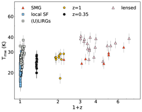
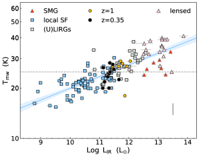
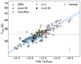
We therefore explore the validity of assuming constant $T_{\rm mw}$ by collating measurements of $T_{\rm mw}$ from the literature (Dunne & Eales, 2001; Hunt et al., 2019), and additionally making our own fits where possible. In Fig. 1 we show that there are indeed strong correlations of $T_{\rm mw}$ with the observables, namely $z$, $L_{\rm IR}$ and the SED colour, $L_{\rm IR}$/$L_{850}$. There is a clear difference between samples with low and high SFRs, with $\langle\mbox{$T_{\rm mw}$}(\rm MS)\rangle=23.0\pm 0.4$ k while $\langle\mbox{$T_{\rm mw}$}(\rm SMG)\rangle=30.1\pm 0.7$ k. We fit empirical relations for the correlations in Fig. 1 (see Table LABEL:fitsT). Where there is no direct estimate of $T_{\rm mw}$ from an SED fit, which is the case for two-thirds of galaxies, we use these empirical relations to derive $T_{\rm mw}$ for use in our subsequent analysis. Appendix H.2 compares our approach, where we use individual estimates of $T_{\rm mw}$, to the adoption of a constant $T_{\rm mw}$=25 k, where we will discuss those findings in §5.

In their work on strongly lensed SMGs at high redshift, which includes dust continuum emission as a constraint in a large-velocity gradient (LVG) model, Harrington et al. (2021) find that $T_{\rm d}$$\sim$ $T_{\rm mw}$ for most SMGs, with both measures of temperature higher than the $T_{\rm mw}$=25 k commonly used in the literature. To ensure consistency with our other estimates of $T_{\rm d}$, we fitted the Harrington et al. (2021) photometry with three simple models: 1) an isothermal optically thin MBB; 2) an MBB with variable optical depth and – where there were enough data – 3) a two-component MBB. In agreement with Harrington et al., we find that a single dust temperature adequately describes the SED of these galaxies, in contrast to lower redshift (U)LIRGs and normal galaxies which are better fit with multiple dust components ($T_{\rm d}$ $>$ $T_{\rm mw}$) and/or fits with higher FIR optical depths. The temperatures from the Harrington et al. turbulence model correlate best with our isothermal $T_{\rm d}$ meansurements for these galaxies, and the temperatures returned when allowing variable optical depth, $\mbox{$T_{\rm d}$}(\tau)$, are always significantly higher than those from the Harrington et al. model. We therefore do not use optically thick fits to yield $T_{\rm mw}$ for our high-redshift SMGs. We instead use two-component SED fits to the lensed Planck sources and the handful of SMGs with sufficient data for the empirical relations shown in Fig. 5.

The other key physical parameter in the dust–H₂ conversion is $\kappa_{\rm H}$, which is a combination of the dust mass absorption coefficient ($\kappa_{850}$) and $\delta_{\rm GDR}$, such that $\kappa_{\rm H}$= $\delta_{\rm GDR}$/$\kappa_{850}$. Briefly, $\kappa_{850}$ is sensitive to the grain composition and structure (amorphous; crystalline; coagulated; mantled), while $\delta_{\rm GDR}$ is roughly proportional to metallicity and, for galaxies with metallicity within a factor 2 of $Z_{\odot}$, as expected for those in our samples, can be taken to be roughly constant, at $\delta_{\rm GDR}$$=100$–150 (Sodroski et al., 1997; Dunne et al., 2000; Dunne & Eales, 2001; Draine et al., 2007; Muñoz-Mateos et al., 2009; Leroy et al., 2011; Sandstrom et al., 2013; Planck Collaboration et al., 2011; Jones et al., 2017; De Vis et al., 2021).

Fortunately, observational measures of $\kappa_{\rm H}$ are available, both for the Milky Way and for external galaxies, with values of $\kappa_{\rm H}$ $\sim 2000$ kg m^-2 in the Milky Way’s diffuse interstellar medium (ISM) and $\kappa_{\rm H}$ $\sim 800$ kg m^-2 in dense clouds. Appendix C discusses in more detail how it is measured, and Table LABEL:kappalitT provides a comprehensive set of observational and theoretical values for $\kappa_{\rm H}$ from the literature.

It is impossible to disentangle the effect of changing dust properties ($\kappa_{850}$) from changes in $\delta_{\rm GDR}$ in observational determinations of $\kappa_{\rm H}$. While the decrease in $\kappa_{\rm H}$ towards denser sightlines in the Milky Way is thought to be due to the dust grains coagulating in denser environments – a process expected to increase their emissivity (e.g. Köhler et al., 2015) – there may also be some decrease in $\delta_{\rm GDR}$ if the gas is accreted into dust mantles or ices (i.e. grain growth). Both effects are to be expected (e.g. Jones et al., 2017; Jones, 2018) and both act to decrease $\kappa_{\rm H}$. Counter to that, the higher estimates of $\kappa_{\rm H}$ in the diffuse atomic phase (lowest $N_{\rm H}$ sightlines at high latitudes) in the Milky Way may be due in part to a lower dust emissivity for grains without ice mantles, where only the refractory cores remain, subjected to harsher ultraviolet (UV) irradiation. Additionally, there is likely a metallicity gradient at high latitudes, leading to a higher $\delta_{\rm GDR}$, further increasing $\kappa_{\rm H}$. There is thus a qualitative expectation that denser regions with higher metallicity will have higher dust emissivity, $\kappa_{850}$, and lower $\delta_{\rm GDR}$, producing a lower $\kappa_{\rm H}$. More diffuse regions with lower metallicity will move in the opposite direction. In §5, we find that we can constrain the range of $\kappa_{\rm H}$, at least, and therefore the combination of $\delta_{\rm GDR}$/$\kappa_{850}$.

2.3.2 $\rm C\,I$–$\rm{H_{2}}$ calibration

Here, we introduce the two physical parameters the $X_{\rm C\,I}$=$\rm[C^{0}/H_{2}]$ average abundance ratio and the average excitation factor $Q_{10}$$=\rm N_{1}/N_{tot}$, pertinent to the use of C i as a tracer of H₂. The relationship between $M_{\rm H2}$ and the ‘observable’ – [C i](1–0) line emission – is (in astronomical units):

$$\mbox{$M_{\rm H2}$}({\rm M}_{\odot})=\frac{0.0127}{X_{\rm C\,I}\,\,Q_{10}}\left(\frac{D_{\rm L}^{2}}{1+z}\right)\,\,\left[\frac{\int_{\Delta V}S_{\rm[CI](1-0)}dv}{\rm Jy\,km\,s^{-1}}\right]$$ (7)

with $D_{\rm L}$ in Mpc and $\int_{\Delta V}S_{\rm[CI](1-0)}\Delta v$ in Jy km s^-1. Expressed in units of line luminosity, this becomes:

$$\mbox{$M_{\rm H2}$}(\mbox{$\rm M_{\odot}$})=\frac{9.51\times 10^{-5}}{\mbox{$X_{\rm C\,I}$}\,Q_{10}}\,\mbox{$L^{\prime}_{\rm C\,I}$}.$$ (8)

The excitation term, $Q_{10}$, describes the relative fraction of carbon atoms in the $J=1$ state. Under general non-LTE conditions it is a function of both gas density, $n$, and $T_{\rm k}$  and is derived analytically in the Appendix to Papadopoulos, Thi & Viti (2004). A recent study of the [C i](2–1)/(1–0) line ratio (Papadopoulos, Dunne & Maddox, 2022) finds that the C i lines are both sub-thermally excited in the ISM of galaxies, with the [C i](2–1) especially so (see also Harrington et al., 2021). Thus the LTE expressions for $Q_{10}$ should not be used, nor will the C i line ratio produce an estimate of $T_{\rm k}$ (both methods having been widely used in the literature to date). Details for $Q_{10}$ are in the Appendix D, but in summary we find:

1. The [C i](1–0) excitation term, $Q_{10}$, is a non-trivial function of density and temperature, but for the range $\mbox{$T_{\rm k}$}\geq 20$ K and log $n\geq 2.5$ – which is where the bulk of H₂ in star forming galaxies is thought to reside – $\langle\mbox{$Q_{10}$}\rangle=0.48\pm 0.08$ where the 99 per cent confidence range is quoted (see Papadopoulos et al. 2022 and Figure 13 for details).

2. Due to a slight super-thermal behaviour, higher density, higher $T_{\rm k}$ conditions can produce similar or even lower $Q_{10}$ than lower density, lower $T_{\rm k}$ conditions. This breaks any intuitive link between $Q_{10}$ and the ISM conditions, i.e. we do not necessarily expect a higher $Q_{10}$ in SMGs compared to MS galaxies (see Fig. 13).

3. As the [C i](2–1) line is even more strongly sub-thermally excited, its $Q_{21}=N_{2}/N_{\rm tot}$ factor varies strongly. This is the main reason why our current study is restricted to the [C i](1–0) line.

As the [C i](${}^{3}P_{1}$–${}^{3}P_{0}$) line is optically thin for most conditions expected in spiral disks (Weiß et al., 2005; Pérez-Beaupuits et al., 2015; Harrington et al., 2021), the relationship between $L^{\prime}_{\rm C\,I}$ and $M_{\rm H2}$ is proportional to $X_{\rm C\,I}$ – the abundance of carbon atoms relative to H₂. This dependence on abundance is as expected for any method that employs tracers of $\rm H_{2}$ gas mass other than the $\rm H_{2}$ lines themselves.

With the excitation factor $Q_{10}$ varying no more than 16 per cent over the typical range of H₂ conditions in galaxies ($\mbox{$T_{\rm k}$}\geq 20$ K, log $n\geq 2.5$), the major source of uncertainty in C i-based molecular gas mass estimates (and thus the major source of scatter in the $\alpha_{\rm C\,I}$ conversion factor) is the neutral carbon abundance, $X_{\rm C\,I}$. The relatively recent introduction of the [C i](1–0) line as a gas tracer means that $X_{\rm C\,I}$ has not been widely explored – constraining it and investigating any potential trends is a key outcome of our cross-calibration work.

In the Milky Way, $X_{\rm C\,I}$ is found to vary only modestly, from 0.8–$2.2\times 10^{-5}$ (e.g. Zmuidzinas et al., 1988; Frerking et al., 1989; Tauber et al., 1995; Ikeda et al., 2002), while a much higher value ($\mbox{$X_{\rm C\,I}$}=5\times 10^{-5}$) has been inferred for the nearby starburst nucleus of M 82 (Schilke et al., 1993; White et al., 1994; Stutzki et al., 1997). Thanks to ALMA, very high localised ratios of $L^{\prime}_{\rm C\,I}$/$L^{\prime}_{\rm CO}$ (translating to high $X_{\rm C\,I}$=5-7$\times 10^{-5}$) have also been measured in extreme regions, such as the Circum-Nuclear Disk (CND) of NGC 7469 which is believed to host an X-ray Dominated Region (XDR) (Izumi et al., 2020) and the outflow region in NGC 6240 (Cicone et al., 2018). More modestly elevated $L^{\prime}_{\rm C\,I}$/$L^{\prime}_{\rm CO}$ ratios tend to be found in the central nuclear regions of starburst galaxies (Jiao et al., 2019; Salak et al., 2019; Saito et al., 2020). However, when averaged over larger kpc scale regions – the ratios become consistent with the average global ratios measured for this sample (see Figure 5). Independent measurements of $\mbox{$X_{\rm C\,I}$}=1.6^{+1.3}_{-0.7}\times 10^{-5}$ (for solar metallicity) were made by Heintz & Watson (2020) using UV absorption measures for a range of absorber systems across cosmic time. Cosmic rays (and X-rays) are expected to dissociate CO in favour of atomic carbon, increasing $[{\rm C}^{0}/{\rm CO}]$, a hypothesis supported by both simulations and observations (e.g. Bisbas et al., 2015; Clark et al., 2019a; Israel, 2020; Izumi et al., 2020).

2.3.3 CO–$\rm{H_{2}}$ calibration

The ¹²CO(1–0) line is optically thick in most (but not all see Aalto et al., 1995, e.g.) ISM conditions expected in galaxies. Unlike dust continuum emission where optical depths build up over large columns of dust, the entire CO line optical depth builds up within very small gas ‘cells’ ($<$0.1 pc) due to the very turbulent nature of the velocity fields, and the small thermal line widths (Tauber et al., 1991; Falgarone et al., 1998). This localised nature of CO line optical depths and the macro-turbulent CO line formation mechanism allows a great simplification of the radiative transfer models of such lines, i.e. the use of the so-called Large Velocity Gradient (LVG) approximation. However, it also complicates the relationship between the CO line luminosity and the underlying $\rm H_{2}$ gas mass, making the corresponding conversion factor, $\alpha_{\rm CO}$, dependent on the thermal state of the gas, its average density, as well as its dynamic state.

Following Papadopoulos et al. (2012b) the $\alpha_{\rm CO}$ factor in an LVG setting is given by:

$$\mbox{$\alpha_{\rm CO}$}=2.65\frac{\sqrt{n_{\rm H2}}}{T_{\rm b}}\,K_{\rm vir}^{-1}\,\,\,\,[\mbox{M${}_{\odot}$\,({\sc k}\,km\,s${}^{-1}$\,pc${}^{2}$)${}^{-1}$}]$$ (9)

where $n_{\rm H2}$ and $T_{\rm b}$ are the average density (in cm^-3) and the CO(1–0) brightness temperature for the molecular cloud ensemble while $K_{\rm vir}$ describes the average dynamic state of the gas (self-gravitating clouds $K_{\rm vir}\sim 1$, unbound clouds $K_{\rm vir}>1$). In principle, multi-phase LVG models of CO (and ¹³CO) SLEDs can be used to constrain $\alpha_{\rm CO}$, but in practice this demands large line datasets per galaxy (e.g. Papadopoulos et al., 2014; Harrington et al., 2021), making it impractical for use in large galaxy samples. This is why in our study $\alpha_{\rm CO}$ remains an empirical conversion factor to be (cross)-calibrated.

2.3.4 Conversion factors and physical parameters

The two optically thin tracers – thermal dust continuum emission and C i  – have a simple relation between the empirical ‘mass-to-light’ conversion parameter ($\alpha_{\rm X}$) and the physical conditions in the ISM (e.g. abundance, emissivity, temperature). We can write the empirical factors (Eqn. 1) in terms of these physical parameters as follows:

$$\mbox{$\alpha_{850}$}=\frac{1.628\times 10^{16}}{1.36\,\mbox{$\kappa_{\rm H}$}}\left(\frac{24.5}{\mbox{$T_{\rm mw}$}}\right)^{-1.4}\,\,\,{\rm W\,Hz}^{-1}{\rm M}_{\rm mol}^{-1}\,\,,$$ (10)

where the factor 1.36 corrects to total molecular mass, including He.

$$\mbox{$\alpha_{\rm C\,I}$}=16.8\,\left[\frac{\mbox{$X_{\rm C\,I}$}}{1.6\times 10^{-5}}\right]^{-1}\left[\frac{Q_{10}}{0.48}\right]^{-1}\,\,\,\rm{\mbox{$\rm M_{\odot}$}\,(K\,km\,s^{-1}\,pc^{2})^{-1}}$$ (11)

Eqn. 11 also includes the factor 1.36 for He.

3 Deriving self-consistent calibration of conversion factors

We next describe how we combine the measurements of multiple gas tracers in the most efficient way, in order to determine their cross-calibrations. Our goal is to find the empirical conversion factors ($\alpha_{850}$, $\alpha_{\rm C\,I}$, $\alpha_{\rm CO}$) or physical parameters ($\kappa_{\rm H}$, $X_{\rm C\,I}$), which produce a consistent estimate for $M_{\rm H2}$ in a given galaxy.

Our dataset provides nested samples, each with a different set of available gas tracers. The daX sample has all three tracers available – dust continuum, CO and C i, and contains 101 galaxies ($N_{\rm daX}$ = 101). The names and statistics for the other samples are as follows: ad – CO and dust, $N_{\rm ad}$ = 326; Xd – C i and dust, $N_{\rm Xd}$ = 140; Xa – C i and CO, $N_{\rm Xa}$ = 109. The properties of these samples are in Table 2.

The best constraints at log₁₀ $L_{\rm IR}$ $>11$ come from the daX sample because it has three independent tracers of gas mass, but it lacks coverage of luminosities below $l_{\rm IR}=11$. The ad sample is the largest and spans the widest range in $L_{\rm IR}$, reflecting the longer time for which CO observations have been possible for nearby galaxies.

We begin with the daX sample, to illustrate the method of optimisation for the estimates of all three conversion factors simultaneously. There are four unknowns namely: $m={\rm log}(\mbox{$M_{\rm H2}$})$, $X={\rm log}(\mbox{$X_{\rm C\,I}$})$, $\kappa={\rm log}(\mbox{$\kappa_{\rm H}$})$, and $\alpha={\rm log}(\mbox{$\alpha_{\rm CO}$})$, and three observables: $L^{\prime}_{\rm CO}$, $L^{\prime}_{\rm C\,I}$ and $L_{850}$.

With an independent measure of the true $M_{\rm H2}$, the observables would provide direct estimates of the three conversion factors; however, the value of $M_{\rm H2}$ is not known a priori, so we must use a probabilistic argument based on the fact the observations do provide constraints on the relative values of the conversion factors for each galaxy. There is thus a set of self-consistent conversion factors which link the observables to the true $M_{\rm H2}$, with an unknown common constant factor.

The Bayesian approach we use is described in detail in Appendix F and requires an estimate of the intrinsic scatter for the logarithms of each of the factors: $s_{\rm X}$, $s_{\kappa}$ and $s_{\alpha}$. The observable luminosities relate to these factors as follows, where the coefficients of proportionality are listed in Table 3:

$$\frac{\mbox{$L^{\prime}_{\rm CO}$}}{\mbox{$L^{\prime}_{\rm C\,I}$}}\propto\mbox{$\alpha_{\rm CO}$}\mbox{$X_{\rm C\,I}$}, \frac{\mbox{$L_{850}$}}{\mbox{$L^{\prime}_{\rm C\,I}$}}\propto\mbox{$\kappa_{\rm H}$}\mbox{$X_{\rm C\,I}$},\, \frac{\mbox{$L^{\prime}_{\rm CO}$}}{\mbox{$L_{850}$}}\propto\frac{\mbox{$\alpha_{\rm CO}$}}{\mbox{$\kappa_{\rm H}$}}.$$ (12)

We begin by measuring the intrinsic scatter between the three pairs of observables using an orthogonal distance regression (ODR) fitting method, which includes the intrinsic scatter, $\lambda$, as a third parameter in the analysis (see Appendix I for full details). The three pair variances derived from the data are then used to estimate the intrinsic variance of the three individual conversion factors (the derivation can be found in Appendix E). The values of the intrinsic scatter for the parameters are given in Table 3, with $X_{\rm C\,I}$ having the smallest scatter between galaxies. This finding is purely empirical, requiring no assumptions about the values or trends of the conversion factors, and as such is very interesting.

Table 2: Samples used in cross-calibration analysis.

Sample Tracers present $N$ median log $L_{\rm IR}$ daX Dust, CO and C i 101  (90) 11.65 (11.77) Xa CO and C i 109  (97) 11.66 (11.88) Xd Dust and C i 140  (128) 11.88 (12.06) ad CO and dust 326  (240) 11.54 (12.07)

Table 3: Summary of the parameters required to reproduce this analysis.

Quantity Set C i CO Dust physical $X_{\rm C\,I}$ $\alpha_{\rm CO}$ $\kappa_{\rm H}$ empirical $\alpha_{\rm C\,I}$ $\alpha_{\rm CO}$ $\alpha_{850}$ $s_{X,\alpha,\kappa}$ log $L_{\rm IR}>11$ 0.082 0.1646 0.1339 BL 0.1125 0.1436 0.1294

Figure 2: Tracer luminosity ratios as a function of lensing, redshift and SFR. $p_{\rm KS}$ is the probability of no difference from a two-sided KS test. Left column: $L_{850}$/$L^{\prime}_{\rm CO}$ – there are no indications of any bias due to lensing or redshift. The third panel shows the effect of high $f_{\rm H\,I}$ in MS galaxies (we have not applied the H i correction factor to show the difference in the raw ratio). The green-shaded region consists of MS galaxies with log $\mbox{$L^{\prime}_{\rm CO}$}>8.9$ and $\mbox{$f_{\rm H\,I}$}<1$. The black line is for all galaxies with $log\mbox{$L^{\prime}_{\rm CO}$}<8.9$, including the lo-VALES galaxies suspected of having $\mbox{$f_{\rm H\,I}$}>1$. Galaxies known to have $\mbox{$f_{\rm H\,I}$}>1$ are shown as the dotted line to illustrate the similarity. The MS sub-group in the lower panel excludes the $\mbox{$f_{\rm H\,I}$}>1$ and lo-VALES galaxies. Middle column: $L_{850}$/$L^{\prime}_{\rm C\,I}$ – there are no indications of bias due to lensing or redshift. The third panel shows the C i^cor galaxies from J19 compared to the rest of the MS sub-group; even with the aperture correction applied to the C i flux (Appendix 4.4), they have a significantly different distribution of observed ratios. In the lower panel, we exclude C i^cor galaxies and find no difference between galaxies with high and low SFRs. Right column: $L^{\prime}_{\rm C\,I}$/$L^{\prime}_{\rm CO}$ – the highest redshift SMGs ($z>3$) have higher $L^{\prime}_{\rm C\,I}$/$L^{\prime}_{\rm CO}$ at marginal significance ($p=0.012$), but there are only 11 galaxies at $z>3$. The third panel shows once more the difference between the C i^cor and other galaxies in both high and low luminosity bins. Even though the C i and CO are measured in the same apertures, the C i^cor galaxies have much lower $L^{\prime}_{\rm C\,I}$/$L^{\prime}_{\rm CO}$. The bottom panel shows a low signficance difference between high and low SFR galaxies ($p=0.056$), becoming significant when including the C i^cor galaxies. Means and KS results are given in Table LABEL:hypT.

As we do not have any independent measure of the gas mass with which to normalise our cross-calibration (four unknowns but only three measurements), we must make an assumption about the sample average of one of the physical or empirical conversion factors. However, with that assumption made transparent, the individual values can always be scaled to whichever normalisation a reader wishes to adopt. The relative values, however, are always the optimal solution.

We choose to use the dust parameter $\kappa_{\rm H}$= $\delta_{\rm GDR}$/$\kappa_{850}$ for this normalisation, because there are no trends of $L_{850}$/$L^{\prime}_{\rm CO}$ or $L_{850}$/$L^{\prime}_{\rm C\,I}$ with $L_{\rm IR}$ (see Figs 2, 14) and $\kappa_{\rm H}$ also has the best observational constraints.

For the Xa sample, where there are no dust continuum measurements, we normalise to $\mbox{$X_{\rm C\,I}$}^{\rm N}=1.6\times 10^{-5}$, which is the mid-range of the values suggested by the independent study of absorption lines by Heintz & Watson (2020).

All the galaxies in our sample are metal rich ($0.5<Z/Z_{\odot}<2$) and so we assume that $\kappa_{\rm H}$ ($\delta_{\rm GDR}$) should be similar to that in the Milky Way and other local disks. Throughout the rest of this work, we will use as our reference point the mid-range of extragalactic determinations, $\kappa_{\rm H}$= 1500–2200 kg m^-2, which are consistent with measurements of the diffuse ISM in the Milky Way. Our chosen normalisation value, then, is $\kappa_{\rm H}$^N = 1884 kg m^-2, which is a good match to current theoretical dust models (THEMIS: Jones et al., 2017, and the updated Draine et al., 2007 modified by Hensley & Draine, 2021).

For the standard Milky Way value of $\delta_{\rm GDR}$ (= 135, Jones et al., 2017; Magdis et al., 2012), $\kappa_{\rm H}$ = 1884 kg m^-2 implies that $\kappa_{850}$ = 0.071 m² kg^-1, similar to that used in many extragalactic studies (Dunne et al., 2000; James et al., 2002; da Cunha et al., 2013). For a $\delta_{\rm GDR}$ fixed to 135, the range of $\kappa_{\rm H}$ in extragalactic studies implies a range in $\kappa_{850}$ of 0.06–0.09 m² kg^-1. Table LABEL:kappalitT lists $\kappa_{\rm H}$ values from extragalactic and Galactic observations, as well as from theoretical dust models.

Note that the choice of normalisation does not affect any of the trends, nor the ratio of the conversion parameters in the pairings; it merely sets the average value of the reference calibration parameter, to which the others are relative.

The sample mean expectation values for the other two parameters, $\langle\mbox{$\alpha_{\rm CO}$}\rangle$ and $\langle\mbox{$X_{\rm C\,I}$}\rangle$, are next derived from our assumed value of $\langle\mbox{$\kappa_{\rm H}$}\rangle$, together with the mean ratios of the observables listed in Table 3. The effective standard deviation is also calculated – the intrinsic scatter of each parameter added in quadrature to the measurement error for that gas tracer. For example, for CO:

$$\sigma_{\rm eff}=\sqrt{s_{\alpha}^{2}+\sigma_{\rm CO}^{2}},$$

where $s_{\alpha}$ is the intrinsic scatter in log($\alpha_{\rm CO}$), and $\sigma_{\rm CO}$ is the measurement error on log($L^{\prime}_{\rm CO}$).

We can now estimate the probability of finding a particular set of conversion factors for any given galaxy. We use $a_{i},\,i=1,2,3$ to denote the logarithms of the three conversion factors, and write the mean expectation values and effective standard deviations as $\langle a_{i}\rangle$, and $\sigma_{i,\rm eff}$ respectively. Assuming that these follow Gaussian distributions, the probability of finding the factors, $a_{i}$, for any galaxy is:

$$P\propto\displaystyle\prod_{i=1}^{N}\exp\left(-\frac{(a_{i}-\langle a_{i}\rangle)^{2}}{2\sigma_{\rm i,eff}^{2}}\right)\\ =\exp\left(-\displaystyle\sum_{i=1}^{N}\frac{(a_{i}-\langle a_{i}\rangle)^{2}}{2\sigma_{\rm i,eff}^{2}}\right).$$ (13)

Thus, the ratios of observable luminosities for any given galaxy can be used to determine the ratios of conversion factors (Eqn. 12), and the common scaling factor that maximises the probability in Equation 13 is the best estimate of $M_{\rm H2}$. The derivation in Appendix F shows that this reduces analytically to a simple inverse variance weighted mean, such that:

$$\log M_{\rm H_{2}}^{\rm opt}=\frac{\sum^{N}_{i=1}(m_{i}\times w_{i})}{\sum^{N}_{i=1}w_{i}},$$ (14)

where $w_{i}=1/\sigma_{i,\rm eff}^{2}$, and $m_{i}$ is the log mass estimate for each tracer.

$$m_{i}=l_{i}+\langle a_{i}\rangle,$$

where $l_{i}$ is the measured observable (log luminosity) and $\langle a_{i}\rangle$ is the sample mean expectation value for the conversion factor. Once the optimal mass is determined this way, we can then estimate the corresponding optimal conversion factor on a per-galaxy basis, as:

$$a_{i}=m^{\rm opt}-l_{i}.$$ (15)

The error on the optimal mass is simply the error on the inverse variance weighted mean:

$$\sigma_{m}^{\rm opt}=\left(\sum^{N}_{i=1}w_{i}\right)^{-1/2},$$ (16)

and the error on each of the conversion factors, accounting for co-variance is:

$$\sigma_{ai}=\sqrt{\sigma_{\rm m^{opt}}^{2}+\sigma_{li}^{2}\left(1-\frac{2w_{i}}{\sum^{N}_{j=1}w_{j}}\right)},$$ (17)

where $\sigma_{li}$ is the logarithmic measurement error on the observable quantity, e.g. $L^{\prime}_{\rm CO}$, $L^{\prime}_{\rm C\,I}$, $L_{850}$.

By design, each tracer for a given galaxy, together with its optimised conversion factors, will produce the same gas mass, such that $\mbox{$M_{\rm H2}$}^{\rm CO}=\mbox{$M_{\rm H2}$}^{\rm C\,I}=\mbox{$M_{\rm H2}$}^{\rm dust}$.

4 Trends in the luminosity ratios

As our cross-calibration process relies on measurements of the luminosity ratios, it is first instructive to look at the trends in these observables to better understand any subsequent trends in the derived conversion factors.

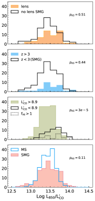
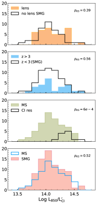
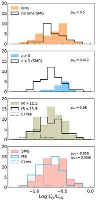
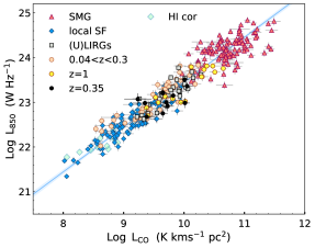
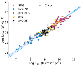
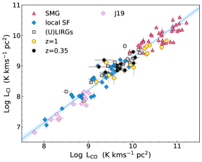
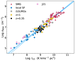
Histograms of the tracer ratios are shown in Fig. 2, split by factors such as lensing, redshift, SFR, and other notable quantities. The correlations of the three tracer luminosities are shown in Fig. 3, where the various samples are colour coded and labelled and in each panel the blue line and shaded region represent the best fit and $2\sigma$ error interval. Fitting was performed using our own Orthogonal Distance Regression (ODR) method, which includes $x$ and $y$ errors, intrinsic scatter as a third parameter, and covariance in errors where required. The method is described in detail in Appendix I. Fit parameters, slope $m$, intercept $c$, and scatter ln $\lambda$ , are listed in Table LABEL:fitsT and statistics for the various subsets from Fig. 2 are given in Table LABEL:hypT. It is instructive to look at these two plots together for the same luminosity pairs.

Figure 3: Relationships between the observed luminosities. The blue line and shaded regions in each panel show the best fit and the $2\sigma$ uncertainty (see Table LABEL:fitsT for parameters). Top left: $L_{850}$–$L^{\prime}_{\rm CO}$. Cyan diamonds indicate those local galaxies which have $f_{\rm H\,I}$ $>1$ and have corrected values of $L_{850}$. The best fit is shown, including the H i-corrected set, but excluding the lo-VALES galaxies (peach circles with log $L^{\prime}_{\rm CO}$ $<8.9$; see Appendix B.1). Choosing only galaxies with $f_{\rm H\,I}$ $<1$ does not change the results; the fit is consistent with a linear slope with a high degree of confidence. Top right: $L_{850}$–$L^{\prime}_{\rm C\,I}$. The resolved C i^cor galaxies from J19 that have an aperture correction (Appendix A) applied to $L^{\prime}_{\rm C\,I}$ in order to compare to $L_{850}$ are shown as pink diamonds. The dotted blue line shows the fit when these galaxies are included. The solid blue line is the fit that excludes these galaxies, while the dashed blue line is the fit to the log $L_{\rm IR}>11$ galaxies only. Bottom left: $L^{\prime}_{\rm C\,I}$–$L^{\prime}_{\rm CO}$. The pink diamonds are the C i^cor galaxies, where now the C i and CO are from matched regions, however, they are still offset to lower $L^{\prime}_{\rm C\,I}$ for a given $L^{\prime}_{\rm CO}$. The fit including the pink diamonds is steeper than linear, while excluding them (solid line) returns a linear slope. Bottom right: $\sigma^{\prime}_{850}$–$L^{\prime}_{\rm C\,I}$. We compare the 850-$\mu$m emissivity ($\mbox{$\sigma^{\prime}_{850}$}=\mbox{$M_{\rm dust}$}\times\mbox{$\kappa_{850}$}$) to $L^{\prime}_{\rm C\,I}$. This allows us to show dust data in the resolved galaxies from Jiao et al. (2021) (pink stars) measured in the same region as [C i](1–0). The dotted blue line shows the fit including the pink stars, the solid line shows the fit excluding the C i^cor galaxies and the dashed line shows the fit to log $L_{\rm IR}>11$ galaxies only. The local resolved (C i^cor) galaxies from J19/J21 appear to have less C i emission for a given dust or CO luminosity, an effect which persists even when comparing matched regions (bottom row).

4.1 $L_{850}$ vs. $L^{\prime}_{\rm CO}$

The left-hand column of Fig. 2 and Fig. 3(a) show the quantities $L_{850}$ vs. $L^{\prime}_{\rm CO}$. There are no significant differences in the distribution of $L_{850}$/$L^{\prime}_{\rm CO}$ with lensing, redshift or SF-mode, but the observed uncorrected ratio is significantly higher for galaxies with log $L^{\prime}_{\rm CO}$ $<8.9$ (Fig. 2; left green histogram). These log $L^{\prime}_{\rm CO}$ $<8.9$ galaxies tend to have optical disks dominated by atomic hydrogen ($f_{\rm H\,I}$ $>1$) and the likely increased contribution to $L_{850}$ from dust associated with H i rather than H₂ results in the offset to higher $L_{850}$/$L^{\prime}_{\rm CO}$ ratios. For local galaxies with $f_{\rm H\,I}$ $>1$ we apply a correction (Appendix B.1) which appears to remove this offset (cyan diamonds in Fig. 3(a)). Galaxies with log $L^{\prime}_{\rm CO}$ $<8.9$ from the VALES sample at $0.04<z<0.3$ (Villanueva et al., 2017; Hughes et al., 2017) have noticeably higher $L_{850}$/$L^{\prime}_{\rm CO}$ ratios than VALES galaxies with log $L^{\prime}_{\rm CO}$ $>8.9$ (peach circles in Fig. 3(a) and Table LABEL:hypT). There are no published H i measurements for VALES, but we suspect that the lo-VALES sample with log $L^{\prime}_{\rm CO}$ $<8.9$ is likely to be H i-rich, based on the similarity between the log $L^{\prime}_{\rm CO}$ $<8.9$ and $f_{\rm H\,I}$ $>1$ categories in the third panel. We therefore exclude lo-VALES from our averages, as we suspect they are in need of a correction for H i but we have no means to apply one. We also recommend that a low $L^{\prime}_{\rm CO}$ requires careful consideration of H i-related dust. In Fig. 3(a), the tracers show a linear dependence, regardless of exactly which galaxies are included (Table LABEL:fitsT). The lo-VALES galaxies are excluded from all the fits.

4.2 $L_{850}$ vs. $L^{\prime}_{\rm C\,I}$

The central column of Fig. 2 and Fig. 3(b) show $L_{850}$ vs. $L^{\prime}_{\rm C\,I}$, the pair with the least scatter ($\ln\lambda$ in Table LABEL:fitsT). There are no significant differences in the distributions of $L_{850}$/$L^{\prime}_{\rm C\,I}$ as a function of lensing, redshift or SF-mode. The $L_{850}$–$L^{\prime}_{\rm C\,I}$ sample has 12 galaxies with large angular sizes from J19 that have only part of their disk detected in C i, denoted C i^cor. To compare $L^{\prime}_{\rm C\,I}$ and $L_{850}$ for these galaxies, we need to apply an aperture correction to their C i fluxes, thereby assuming that their $L^{\prime}_{\rm C\,I}$/$L^{\prime}_{\rm CO}$ ratios remain roughly constant across the disk (see Appendix 4.4). Some of the correction factors are very large (up to 0.7 dex); even after correction, their $L_{850}$/$L^{\prime}_{\rm C\,I}$ ratios are significantly offset from the rest of the MS sample (green histogram). Fig. 3(b) shows $L_{850}$ vs. $L^{\prime}_{\rm C\,I}$, with the C i^cor galaxies as pink diamonds. The fit to all galaxies including the C i^cor subset is shown as a dotted blue line, and has a sub-linear slope $m$ ($3\sigma$), although the difference is very small ($m=0.937\pm 0.020$). Excluding the C i^cor galaxies from the fit leaves a linear relationship, shown by the blue solid line. At first glance, this and the green histogram in Fig. 2 suggest that our CO-based corrections are insufficient; however, Fig. 3(d) shows that the problem is not simply the assumption used to correct $L^{\prime}_{\rm C\,I}$ to match the global $L_{850}$. This plot shows the dust emissivity cross-section, $\sigma^{\prime}_{850}$, equivalent to $L_{850}$ but with the temperature sensitivity removed. Importantly, this quantity is measured in the same aperture as $L^{\prime}_{\rm C\,I}$. The C i^cor galaxies are shown as pink stars, and they – along with many other low-luminosity galaxies in J21 – still appear to have less C i emission for a given amount of dust.

Table 4: Parameters of robust ODR fits between variables using MCMC, co-variant errors and including intrinsic scatter, $\ln\lambda$.

Log $x$ Log $y$ Group $m$ $c$ ln $\lambda$ $r_{\rm s}$ $p$ $N$ $L^{\prime}_{\rm CO}$ $L^{\prime}_{\rm C\,I}$ BL 1.023 (0.029) $-0.93$ (0.29) $-2.09$ (0.09) 0.94 109 $L^{\prime}_{\rm CO}$ $L^{\prime}_{\rm C\,I}$ BL+C i^cor 1.078 (0.026) $-1.49$ (0.25) $-2.03$ (0.09) 0.96 121 $L^{\prime}_{\rm CO}$ $L^{\prime}_{\rm C\,I}$ log $L_{\rm IR}>11$ 0.950 (0.035) $-0.18$ (0.37) $-2.07$ (0.10) 0.92 97 $L^{\prime}_{\rm C\,I}$ $L_{850}$ BL 0.976 (0.024) 14.33 (0.23) $-2.11$ (0.09) 0.95 140 $L^{\prime}_{\rm C\,I}$ $L_{850}$ BL+C i^cor 0.937 (0.020) 14.71 (0.19) $-2.08$ (0.08) 0.96 152 $L^{\prime}_{\rm C\,I}$ $L_{850}$ log $L_{\rm IR}>11$ 1.024 (0.030) 13.86 (0.30) $-2.17$ (0.09) 0.94 128 $L^{\prime}_{\rm C\,I}$ $\sigma^{\prime}_{850}$ BL 1.024 (0.025) $-2.28$ (0.24) $-2.05$ (0.08) 0.95 140 $L^{\prime}_{\rm C\,I}$ $\sigma^{\prime}_{850}$ BL+C i^cor 0.997 (0.021) $-2.01$ (0.20) $-2.07$ (0.08) 0.96 152 $L^{\prime}_{\rm CO}$ $L_{850}$ BL 1.003 (0.015) 13.42 (0.15) $-2.01$ (0.05) 0.96 326 $L^{\prime}_{\rm CO}$ $L_{850}$ $f_{\rm H\,I}$<1 1.002 (0.017) 13.43 (0.16) $-1.99$ (0.05) 0.96 310 $L^{\prime}_{\rm CO}$ $L_{850}$ log $L_{\rm IR}>11$ 0.983 (0.026) 13.63 (0.26) $-1.91$ (0.06) 0.93 226 $L_{\rm IR}$ $L^{\prime}_{\rm C\,I}$/$L^{\prime}_{\rm CO}$ BL+C i^cor 0.071 (0.02) $-1.57$ (0.23) $-1.70$ (0.09) 0.26 0.005 121 $L_{\rm IR}$ $L^{\prime}_{\rm C\,I}$/$L^{\prime}_{\rm CO}$ BL 0.034 (0.02) $-1.11$ (0.25) $-1.70$ (0.09) 0.09 0.34 109 $T_{\rm d}$ $L^{\prime}_{\rm C\,I}$/$L^{\prime}_{\rm CO}$ BL+C i^cor 1.23 (0.23) $-2.60$ (0.35) $-$2.20 (0.12) 0.31 115 $T_{\rm d}$ $L^{\prime}_{\rm C\,I}$/$L^{\prime}_{\rm CO}$ BL 0.83 (0.28) $-2.0$ (0.4) $-$2.00 (0.15) 0.15 0.12 103 $L_{\rm IR}$/$L_{850}$ $T_{\rm mw}$ 0.216 (0.010) 3.90 (0.12) $-3.76$ (0.15) 0.82 152 $L_{\rm IR}$ $T_{\rm mw}$ 0.070 (0.004) 0.60 (0.05) $-3.10$ (0.10) 0.80 152 $L_{\rm IR}$ $\alpha_{850}$ BL 0.045 (0.007) 12.271 (0.082) $-3.36$ (0.30) 0.46 230 $L_{\rm IR}$ $\alpha_{\rm CO}$ BL 0.59 (0.09) $-0.91$ (1.10) $-1.00$ (0.50) 0.46 230 $L_{\rm IR}$ $\alpha_{\rm C\,I}$ BL $-0.052$ (0.010) 1.896 (0.124) $-3.90$ (0.20) $-0.48$ 82 $L_{\rm IR}$ $X_{\rm C\,I}$ BL $0.028$ (0.011) $-5.136$ (0.133) $-3.70$ (0.23) 0.29 0.008 82

Table 5: Two-sample KS-test result and Z-test statistic for the following parameter pairs shown in Figs 2 and 4.

Quantity $A$ $N_{\rm A}$ $B$ $N_{\rm B}$ $\bar{A}$ $\bar{B}$ $Z(\sigma)$ $P_{\rm KS}$ $L_{850}$/$L^{\prime}_{\rm CO}$^† log $L^{\prime}_{\rm CO}$<8.9 50 $L^{\prime}_{\rm CO}$>8.9 (MS) 138 $13.600\pm 0.030$ $13.420\pm 0.016$ 5.3 3e-5 $L_{850}$/$L^{\prime}_{\rm CO}$^† $f_{\rm H\,I}$<1 (MS) 168 $f_{\rm H\,I}$>1 (MS) 24 $13.456\pm 0.014$ $13.685\pm 0.042$ 5.2 3e-6 $L_{850}$/$L^{\prime}_{\rm CO}$^† lo-VALES 7 $f_{\rm H\,I}$>1 17 $13.741\pm 0.061$ $13.663\pm 0.053$ 0.57 $L_{850}$/$L^{\prime}_{\rm CO}$ $f_{\rm H\,I}$<1 (MS) 168 $f_{\rm H\,I}$>1 (MS^∗) 17 $13.456\pm 0.014$ $13.448\pm 0.039$ 1.0 $L_{850}$/$L^{\prime}_{\rm C\,I}$ MS 61 C i^cor 12 $14.108\pm 0.027$ $14.36\pm 0.036$ 5.6 6e-4 $L^{\prime}_{\rm C\,I}$/$L^{\prime}_{\rm CO}$ $z<3$ (SMGs) 37 $z>3$ 11 $-0.686\pm 0.031$ $-0.512\pm 0.044$ 3.2 0.012 $L^{\prime}_{\rm CO}$/$L^{\prime}_{\rm C\,I}$ MS 55 SMGs 54 $-0.743\pm 0.028$ $-0.651\pm 0.028$ 2.3 0.056 $L^{\prime}_{\rm CO}$/$L^{\prime}_{\rm C\,I}$ MS+C i^cor 66 SMGs 54 $-0.786\pm 0.026$ $-0.651\pm 0.028$ 3.5 0.006 $T_{\rm d}$ MS 174 SMGs 160 $31.1\pm 0.4$ $38.3\pm 0.7$ 8.8 2e-12 $T_{\rm mw}$ MS 82 SMGs 52 $23.0\pm 0.4$ $30.1\pm 0.7$ 8.8 7e-13

4.3 $L^{\prime}_{\rm C\,I}$ vs. $L^{\prime}_{\rm CO}$

The right-hand column of Fig. 2 and Fig. 3(c) show $L^{\prime}_{\rm C\,I}$ vs. $L^{\prime}_{\rm CO}$. There are no significant differences in $L^{\prime}_{\rm C\,I}$/$L^{\prime}_{\rm CO}$ for strongly lensed vs. unlensed sources, but the highest redshift, $z>3$, galaxies have higher $L^{\prime}_{\rm C\,I}$/$L^{\prime}_{\rm CO}$ ratios at marginal significance ($p=0.012$). There are only 11 galaxies at $z>3$ and a larger sample is needed to determine if this is a genuinely significant trend. Fig. 3(c) shows the C i^cor galaxies as pink diamonds, where the C i and CO fluxes are measured in the same apertures by J19. The solid line shows the fit to all galaxies, which is non-linear at 3$\sigma$ significance ($m=1.078\pm 0.026$). The slope becomes linear once the C i^cor galaxies are removed. The green histogram in Fig. 2 (right) shows more clearly why we see this: the C i^cor galaxies have significantly lower $L^{\prime}_{\rm C\,I}$/$L^{\prime}_{\rm CO}$ ratios compared to other galaxies at similar or higher luminosity. The bottom histogram shows a marginal difference between galaxies with different SFRs ($p=0.056$) when excluding the C i^cor galaxies, which becomes significant when they are included ($p=0.006$).

4.4 Resolved C i fluxes from Herschel FTS mapping

The local resolved galaxies observed with Herschel FTS (Jiao et al., 2019) lie off the global trends seen in Fig. 3. There are possible physical explanations why lower luminosity, and more quiescently star-forming galaxies might have lower C i/CO line ratios (for example, different ISM environments in terms of their position in the CR energy density vs average molecular gas density diagram: see Figure 1 in Bisbas et al., 2015). Low ratios of $L^{\prime}_{\rm C\,I}$/$L^{\prime}_{\rm CO}$ have been found in other studies, most intriguingly in the case of the interacting LIRG NGC 6052 using ALMA (Michiyama et al., 2020), and some high-$z$ strongly lensed sources (Harrington et al., 2021). Such ratios tend to be unusual in higher luminosity samples, however, whereas the resolved FTS sample has a very low average for the C i line ratios with both CO and dust.

We recommend caution in the interpretation of the data for these resolved FTS sources because another team subsequently presented the same data but drew different conclusions (Crocker et al., 2019). We can therefore only note that the C i fluxes from Herschel FTS mapping datasets are not always consistent when analysed by different teams. As these resolved FTS measurements are essentially the only source of C i data at log $L_{\rm IR}<11$, and carry a lot of weight in $L_{\rm IR}$ and SFR correlations, we chose not to include the C i^cor galaxies in the statistical analysis. If, instead, we take the J19 measurements at face value – they signpost a fundamental physical change in C i properties, a finding which clearly warrants further study with ground-based facilities. We discuss possible physical mechanisms for changes in the $L^{\prime}_{\rm C\,I}$/$L^{\prime}_{\rm CO}$and $L^{\prime}_{\rm C\,I}$/$L_{850}$ ratios in Appendix B.2.

4.5 Trends with global indicators of star-formation.

Figure 4: Histograms of (top) luminosity-weighted dust temperature ($T_{\rm d}$) from MBB fits (bottom) mass-weighted dust temperature ($T_{\rm mw}$) from fits allowing for multiple dust temperatures. Means and KS test results are given in Table LABEL:hypT.

Figure 5: $L^{\prime}_{\rm C\,I}$/$L^{\prime}_{\rm CO}$ luminosity ratio (equivalent to $\alpha_{\rm CO}$/$\alpha_{\rm C\,I}$) as a function of luminosity-weighted (peak SED) dust temperature (left) and log $L_{\rm IR}$ (right). The yellow shaded regions in the right panel represent the 1$\sigma$ range of values found by Crocker et al. (2019) for resolved galaxies mapped with the Herschel FTS. The vertical red and blue bars show the 1$\sigma$ range of values for QSOs/SMGs and the Milky Way, respectively (Walter et al., 2011; Frerking et al., 1989). The best fit to all galaxies and 2$\sigma$ confidence region are shown as the blue line and shaded area (parameters are given in Table LABEL:fitsT). The $L^{\prime}_{\rm C\,I}$/$L^{\prime}_{\rm CO}$ ratio has a significant correlation with both $T_{\rm d}$ and log $L_{\rm IR}$ when all galaxies are included, but when excluding the C i^cor galaxies, the correlation all but disappears (blue dotted line).

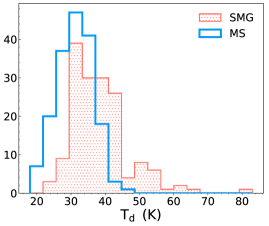
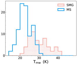
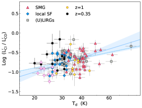
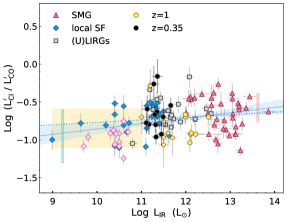
Finally, we check to see if any of the tracer ratios are sensitive to SFR indicators. In our data-set the dust observables $L_{\rm IR}$ and $T_{\rm d}$ are indicators of the intensity and magnitude of star formation in galaxies (e.g. Kennicutt, 1998; Foyle et al., 2012; Liu et al., 2021). As expected, the distribution of $T_{\rm d}$ is very different for the MS galaxies and SMGs (Fig. 4 and Table LABEL:hypT), reflecting the increase in the intensity of star formation in the SMGs. The only tracer ratio sensitive to these SF indicators is $L^{\prime}_{\rm C\,I}$/$L^{\prime}_{\rm CO}$, which in Figure 5 is seen to increase with $L_{\rm IR}$ and $T_{\rm d}$ when all galaxies are considered. Such a trend was not reported for smaller samples over a more limited range of luminosity (e.g. Jiao et al., 2017; Jiao et al., 2019), presumably because of limited statistics. However, if the C i^cor galaxies (pink diamonds) are excluded, the correlation all but disappears (blue dotted line).

Naively, we might expect $L^{\prime}_{\rm C\,I}$/$L^{\prime}_{\rm CO}$ to rise with increasing SFR intensity, due to the expected destruction of CO by cosmic rays (CR) in high-SFR environments (e.g. Bisbas et al., 2015). For a given range of H₂ densities in the typically hierarchical molecular clouds, any increased CR-induced ionisation rate, $\zeta_{\rm CR}$ (due to a rising average CR energy density, $U_{\rm CR}$) will destroy CO in the lower-density, more extended areas, while leaving CO still tracing H₂ in the more compact, denser regions (see also Figure 1 of Papadopoulos et al., 2018 for a visual effect of this). Intriguingly, the gas density, $n$(H₂), and CR ionization rate, $\zeta_{\rm CR}$, will compete against each other in ULIRG/SMG environments, with the higher <n> expected in their highly turbulent ISM tending to keep the ordinary CO/C i chemistry in place, even when exposed to the higher $\zeta_{\rm CR}$  values. Guessing which one will win this highly non-linear competition (see Fig 1, 8 in Bisbas et al., 2015) is dangerous in the absence of CO and C i line data. These effects have been probed with a variety of simulations (e.g. Bisbas et al., 2015, 2021; Clark et al., 2019a; Gong et al., 2020) and while showing similar trends, they are not easily parameterisable in terms of $n$(H₂) and $\zeta_{\rm CR}$; one reason why such cross-calibration efforts of the available gas mass tracers are so important.

The other two tracer ratios show no trends with either $L_{\rm IR}$, $T_{\rm d}$ (our proxies for SFR) – we present the relevant plots in Appendix 14 for completeness.

5 Results

In this section we present the results of the optimisation method, firstly for the daX sample, for which we have all three gas tracers, and later for the other three samples, for which we have pairs of tracers. We investigate trends of the conversion factors with $L_{\rm IR}$ and SFR. Mean values for the conversion factors are listed in Table LABEL:caloptT.

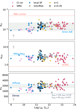
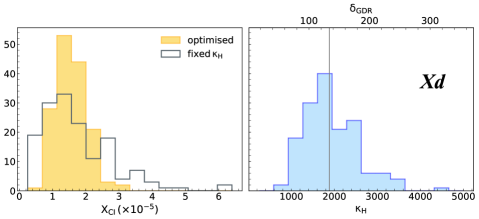
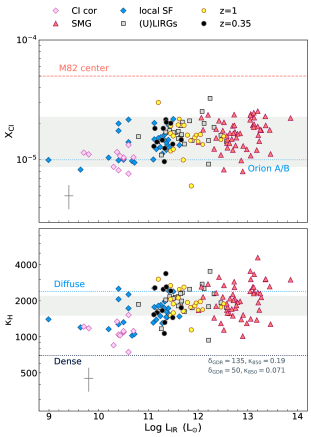
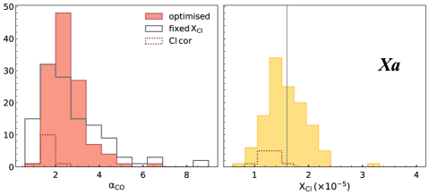
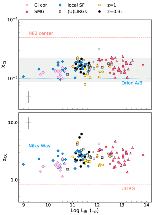
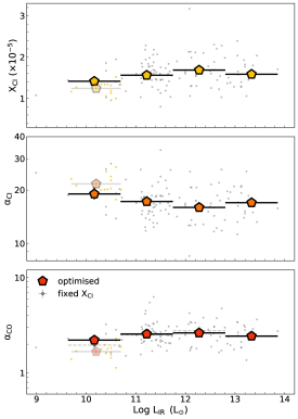
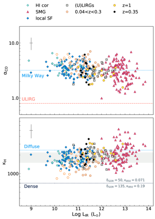
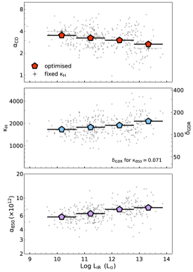
Fig. 6 shows the results for the daX sample (Figs 7–9 present the same results for each of the samples in turn). The top row of each plot shows the distribution of the relevant physical parameter for C i and dust, and the conversion factor for CO: $X_{\rm C\,I}$, $\kappa_{\rm H}$ and $\alpha_{\rm CO}$. The lower left panels show the same quantities for the individual galaxies as a function of $L_{\rm IR}$; each panel indicates a reference measure to give context. For $X_{\rm C\,I}$, the horizontal lines indicate the measured extremes found in the local Universe: Orion A/B clouds in the Milky Way (Ikeda et al., 2002) and the starburst centre of M 82 (White et al., 1994), while the grey shaded region shows the range of values inferred from observations of GRB hosts and QSO absorbers for solar metallicity by Heintz & Watson (2020). They use a method which does not rely on emission measures of dust, CO or C i and so can be considered independent. For $\alpha_{\rm CO}$, the horizontal lines indicate the typical $\alpha_{\rm CO}$ for the Milky Way (Bolatto et al., 2013) and that commonly adopted for ULIRGs and SMGs (Downes & Solomon, 1998). For $\kappa_{\rm H}$, we show a shaded band indicating the range derived for local galaxies (see Table LABEL:kappalitT), along with lines showing the value for the most diffuse and dense sight lines in the Milky Way (Remy et al., 2017). The right lower panels show the running log-means as a function of $L_{\rm IR}$ to make it easier to see any trends, and additionally includes the empirical parameters, $\alpha_{\rm C\,I}$ and $\alpha_{850}$. The solid shaded bins are the means for the grey points, which are those used to determine the calibration; the yellow points are C i^cor and the semi-transparent pentagon is the mean of those – see §4.4 for more details.

Fig. 6 shows that for galaxies with log $L_{\rm IR}>11$ there are only weak trends of the conversion factors with $L_{\rm IR}$. While the normalisation ($\mbox{$\kappa_{\rm H}$}^{\rm N}=1884$ kg m^-2) was chosen to produce average dust properties consistent with the Milky Way and other nearby spirals, the CO and C i conversion factors derived from the luminosity ratios also lie within the ranges expected from independent studies. The averages at log $L_{\rm IR}<11$ are based on only a small number of points (12) and more C i studies are required to probe quiescent local galaxies.

Figure 6: Top row: Distributions of the three conversion factors, $X_{\rm C\,I}$, $\alpha_{\rm CO}$ and $\kappa_{\rm H}$ for the daX sample. The overall normalisation has been set as $\mbox{$\kappa_{\rm H}$}^{\rm N}=1884$ kg m^-2, which produces the $\mbox{$\delta_{\rm GDR}$}=135$ of the Milky Way for $\mbox{$\kappa_{850}$}=0.071$ m² kg^-1(Jones, 2018). The intrinsic pairwise scatter and conversion factors were estimated excluding C i^cor and lo-VALES galaxies. Lower left: The optimised conversion factors as a function of $L_{\rm IR}$. The grey shaded band represents $X_{\rm C\,I}$ at solar metallicity using the relationship found in GRB and QSO absorber hosts by Heintz & Watson (2020), a measure which is independent of assumptions about $\alpha_{\rm CO}$ or $\delta_{\rm GDR}$. Lower right: The running means of the conversion factors, with error bars of $\sigma/\sqrt{N_{\rm bin}}$. The solid shaded bins are the means for the grey points which are those used to determine the calibration, the yellow points are C i^cor and the semi-transparent pentagon is the mean of those – see §4.4 for more details.

Table 6: Mean optimised conversion factors for our various samples.

Sample Selection $N$ $X_{\rm C\,I}$ $\sigma_{\bar{X}}$ $\alpha_{\rm CO}$ $\sigma_{\bar{\alpha}}$ $\kappa_{\rm H}$ $\sigma_{\bar{\kappa}}$ $\delta_{\rm GDR}$ /$\times 10^{-5}$ M_⊙ (k km s^-1 pc²)^-1 m² kg^-1 daX log $L_{\rm IR}>11$ 90 $1.59^{+0.45}_{-0.38}$ 0.04 $2.66^{+0.96}_{-0.70}$ 0.10 $1990^{+738}_{-607}$ 86 141 daX log $L_{\rm IR}<11$ 12 $1.18^{+0.60}_{-0.29}$ 0.13 $2.44^{+0.56}_{-0.51}$ 0.17 $1571^{+732}_{-525}$ 163 112 Xd log $L_{\rm IR}>11$ 128 $1.59^{+0.47}_{-0.35}$ 0.04 $1946^{+654}_{-464}$ 53 138 Xd log $L_{\rm IR}<11$ 12 $1.24^{+0.57}_{-0.27}$ 0.13 $1503^{+604}_{-369}$ 145 107 ad log $L_{\rm IR}>11$ 240 $3.08^{+1.32}_{-0.81}$ 0.07 $1936^{+658}_{-504}$ 45 137 ad log $L_{\rm IR}<11$ 88 $3.52^{+0.95}_{-0.84}$ 0.10 $1718^{+502}_{-339}$ 44 122 Xa log $L_{\rm IR}>11$ 97 $1.61^{+0.39}_{-0.31}$ 0.04 $2.57^{+0.71}_{-0.62}$ 0.08 Xa log $L_{\rm IR}<11$$+$C i^cor 24 $1.30^{+0.2}_{-0.23}$ 0.05 $1.88^{+0.41}_{-0.34}$ 0.10 Xa log $L_{\rm IR}<11$ 12 $1.37^{+0.34}_{-0.31}$ 0.09 $2.11^{+0.18}_{-0.57}$ 0.15

5.1 A calibration for the gas masses

We next give a prescription for estimating gas mass, tailored to how many tracers are available and – where appropriate – the type of galaxy being investigated.

5.1.1 Dual-band

While the information content is greatest for the daX sample, which has three tracer pairs to optimise, the method presented in §3 still improves the cross-calibration for samples which have two tracer measurements, i.e. one pair. The results for the Xd, Xa and ad samples are shown in Figs 7–9 and behave similarly to the daX sample, as one would hope given that the daX galaxies are a subset of the others. The pink diamonds in the lower-left panels in Figs 7 and 8 denote the C i^cor galaxies. The cyan diamonds in the lower-left panel of Fig. 9 are galaxies with $f_{\rm H\,I}$>1 which have been corrected for the contribution of dust mixed with the H i gas, as described in Appendix A. The open peach circles are the lo-VALES galaxies, which we suspect to have $f_{\rm H\,I}$>1 (see §4.1) but which we cannot correct. We do not include these in any averages or histograms.

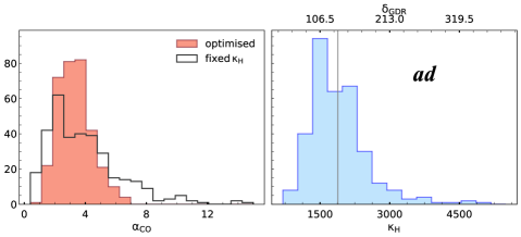
The method previously used in the literature (e.g. Alaghband-Zadeh et al., 2013; Scoville et al., 2016; Orellana et al., 2017; Hughes et al., 2017; Valentino et al., 2018) has been to assume one tracer in a pair (e.g. $L^{\prime}_{\rm CO}$) has a known conversion ($\alpha_{\rm CO}$), then to fix that factor for all galaxies in order to estimate the second (i.e. the one of interest). We show this simple method alongside our optimal method as grey lines and dashed grey error bars in the relevant panels of Figs 7–9. The scatter in the conversion factors for the optimised estimates are governed by the intrinsic scatter we inferred in our analysis of the data in Appendix E, free of assumptions. In contrast, the simple method proscribes that there is no scatter in the known conversion factor, and therefore all of the intrinsic scatter in the luminosity ratio is attributed to the second conversion factor of interest. The optimised method presented here does not assume an ad hoc preference for any particular conversion factor: as it is based on empirical variance analysis, it uses more of the available information to improve the accuracy of the estimated conversion factors. The histograms in Figs (7–9) show that the scatter in the factor of interest is larger when using the simple method, and the trends in the running medians are also more exaggerated.

Comparing the parameter estimates using three tracers to those using two tracers for the same galaxies allows us to test the accuracy of these two-tracer estimates. The details are in Appendix H, but in summary there is a reasonable correlation between the three-tracer and two-tracer estimates, without bias (Fig. 15) and an average scatter of 0.06–0.08 dex.

Figure 7: Top: Distributions of $X_{\rm C\,I}$ and $\kappa_{\rm H}$ for the Xd sample, where the normalisation used is $\mbox{$\kappa_{\rm H}$}^{\rm N}=1884$ kg m^-2. Left: Optimised conversion factors as a function of $L_{\rm IR}$ for the galaxies in the Xd sample. The grey shaded bands represent the range of $X_{\rm C\,I}$ ($Z=Z_{\odot}$) from a study of GRB and QSO absorber hosts by Heintz & Watson (2020), a measure which is independent of assumptions about $\alpha_{\rm CO}$ or $\delta_{\rm GDR}$, and also the range of $\kappa_{\rm H}$ in nearby galaxies. Right: Running means of the conversion factors with error bars of $\sigma/\sqrt{N_{\rm bin}}$. The solid coloured pentagons are the means for the grey points, which are those used to determine the conversion; the yellow points are the C i^cor galaxies and the semi-transparent pentagon is the mean of those (see §4.4 and Appendix B.2). The grey dashed error bars in the $X_{\rm C\,I}$ running mean are for the so-called simple method, where $\mbox{$\kappa_{\rm H}$}=1884$ kg m^-2 is fixed for all galaxies.

Figure 8: Top: Distributions of $X_{\rm C\,I}$ and $\alpha_{\rm CO}$ for the Xa sample, where the normalisation has been set to $\mbox{$X_{\rm C\,I}$}^{\rm N}=1.6\times 10^{-5}$ – the middle of the range for $Z_{\odot}$ found in GRB hosts and QSO absorbers by Heintz & Watson (2020). Lower left: Optimised conversion factors as a function of $L_{\rm IR}$ for the galaxies in the Xa sample. Right: Running means of the conversion factors with error bars of $\sigma/\sqrt{N_{\rm bin}}$. The solid coloured pentagons are the means for the grey points which are those used to determine the conversion; the yellow points represent the C i^cor galaxies and the semi-transparent pentagon is the mean of those – see §4.4 and Appendix B.2. The grey dashed error bars in the $\alpha_{\rm CO}$ running mean are for the so-called simple method, where $\mbox{$X_{\rm C\,I}$}=1.6\times 10^{-5}$ is fixed for all galaxies.

Figure 9: Top: Distributions of $\alpha_{\rm CO}$ and $\delta_{\rm GDR}$ for the ad sample, where the normalisation has been set to $\mbox{$\kappa_{\rm H}$}^{\rm N}=1884$ kg m^-2. Lower left: Optimised conversion factors as a function of $L_{\rm IR}$ for the galaxies in the ad sample. The cyan diamonds indicate galaxies with $f_{\rm H\,I}$>1 which have been corrected for the contribution of dust mixed with H i, following the procedure outlined in Appendix B.1. The open peach circles are the lo-VALES galaxies which we suspect have $f_{\rm H\,I}$>1 – these are not included in the analysis. Right: Running means of the conversion factors with error bars of $\sigma/\sqrt{N_{\rm bin}}$. The coloured points reflect the optimised results and the grey dashed error bars for the $\alpha_{\rm CO}$ running mean are for the so-called simple method, where $\mbox{$\kappa_{\rm H}$}=1884$ kg m^-2 is fixed for all galaxies.

Thus, when multiple H₂ tracers are available, we recommend the procedure outlined in the example below.

Example:

Take the example of a galaxy with observations of both dust and CO. We take the mean value for the appropriate pair combination from Table 3: $\alpha_{\rm CO}$/$\kappa_{\rm H}$=0.00133. For our adopted sample mean normalisation of $\kappa^{\rm N}=1884$ kg m^-2, we now infer the sample mean expectation value of $\langle\alpha\rangle=0.00133\times 1884=2.5$ (excluding He). The sample means, $\kappa^{\rm N}$ (assumed) and $\langle\alpha\rangle$ (derived), are next used to estimate an initial gas mass for our galaxy in each of the two tracers, $L_{850}$ and $L^{\prime}_{\rm CO}$.

$$M_{\kappa}=\kappa^{\rm N}\mbox{$L_{850}$}/4\pi B(\nu_{850},\mbox{$T_{\rm mw}$})\\ M_{\alpha}=\langle\alpha\rangle\mbox{$L^{\prime}_{\rm CO}$}\\$$ (18)

Next, we calculate the effective standard deviation by adding the observational error on the tracer luminosities in quadrature to the intrinsic scatter for $\alpha$ and $\kappa$.

$$\sigma^{\kappa}_{\rm eff}=\sqrt{s_{\kappa}^{2}+\sigma_{850}^{2}}\\ \sigma^{\alpha}_{\rm eff}=\sqrt{s_{\alpha}^{2}+\sigma_{\rm CO}^{2}}\\$$ (19)

where $\sigma_{850}$, $\sigma_{\rm CO}$ are the errors on $\log(\mbox{$L_{850}$})$ and $\log(\mbox{$L^{\prime}_{\rm CO}$})$, and $s_{\kappa}$ and $s_{\alpha}$ are the intrinsic scatter on $\log(\mbox{$\kappa_{\rm H}$})$ and $\log(\mbox{$\alpha_{\rm CO}$})$ listed in Table 3. The optimal H₂ mass estimate is then calculated thus:

$$M^{\rm opt}=\frac{M_{\kappa}/\sigma^{2}_{\rm\kappa,eff}+M_{\alpha}/\sigma^{2}_{\rm\alpha,eff}}{1/\sigma^{2}_{\rm\kappa,eff}+1/\sigma^{2}_{\rm\alpha,eff}}$$ (20)

We now work back to find the optimal conversion parameters for this galaxy:

$$\mbox{$\kappa_{\rm H}$}^{\rm opt}=\kappa^{\rm N}M^{\rm opt}/M_{\kappa}\\ \mbox{$\alpha_{\rm CO}$}^{\rm opt}=\langle\alpha\rangle M^{\rm opt}/M_{\alpha}.\\$$ (21)

Figure 10: Correlations of the empirical calibration factors with their tracer luminosity. The largest sample was used in each case: ad (top and bottom); Xd (top centre). For $\alpha_{850}$ (top), we include the relationship from Scoville et al. (2016), exactly as quoted in that paper. Parameters for the median posterior fit (dark blue line), accounting for co-variance in the errors, are quoted in the legend, and we include 100 random fits from sampling the posterior as pale blue lines to show the scatter. Further details are given in Table LABEL:calfitsT. All tracers have a significant correlation with their tracer luminosity.

[]figs/python/cal_empirical_daX(0.39,0.39)

[]figs/python/cal_empirical_Xa(0.33,0.33) []figs/python/cal_empirical_Xd_kh_fullMS(0.33,0.33) []figs/python/cal_empirical_aod_kh(0.33,0.33)

Figure 11: The empirical conversion factors, $\alpha_{\rm CO}$, $\alpha_{\rm C\,I}$ and $\alpha_{850}$, separately for MS galaxies and SMGs. The blue line histograms represent the MS galaxies. The dark blue dashed lines show the $f_{\rm H\,I}$>1 and C i^cor galaxies. We keep these separate because the corrections are uncertain and the C i^cor galaxies are significantly different in their distributions to the rest of the MS galaxies, as discussed in §4.4. The SMG histograms are shown in red. The result of two-sample KS tests are shown on each panel for each of the comparisons (MS galaxies vs. SMGs). The main comparison between MS galaxies and SMGs is shown first; below, in parentheses, are the results for comparison between the robust MS galaxies and those requiring the corrections described above. daX: Only $\alpha_{\rm C\,I}$ shows a significant ($3.2\sigma$) difference between the two groups, decreasing to $1.9\sigma$ if constant $T_{\rm mw}$=25 k is used. Xa: There is a marginal difference in $\alpha_{\rm C\,I}$ (2.5–$2.9\sigma$) but no difference in $\alpha_{\rm CO}$. There is a significant difference between the C i^cor and other MS galaxies (dotted blue line and parentheses), which cannot be attributed to uncertain aperture corrections as CO and C i are measured in the same aperture. Xd: For $\alpha_{\rm C\,I}$ (and $\kappa_{\rm H}$ – see Table 8) there is a marginal difference (2.6–$3.0\sigma$) between the MS galaxies and SMGs, where these differences vanish when using fixed $T_{\rm mw}$=25 k. There is no difference between MS galaxies and SMGs for $\alpha_{850}$. ad: There is a small ($\sim 10$ per cent) difference in the mean $\alpha_{\rm CO}$ between the MS galaxies and SMGs, significant at the $3.5\sigma$ level. This drops to $2.5\sigma$ when comparing only log $L_{\rm IR}>11$ MS galaxies, and drops further when using constant $T_{\rm mw}$=25 k. We conclude that this is a luminosity-driven effect, not a property of the star-formation mode per se. The difference in $\alpha_{850}$ is highly significant (as is the diference in $\kappa_{\rm H}$, to a lesser extent – see Table 8). Fig. 10 shows that this difference is the result of a steady change in $\alpha_{850}$ with $L_{\rm IR}$ (or $L_{850}$), rather than being a bi-modal split between MS galaxies and SMGs.

5.1.2 Single band: empirical conversion factors

Table 7: Empirical conversion factors recommended for use when only a single gas tracer observation is in hand. These include a factor 1.36 to account for He.

Sample $\alpha_{850}$($\times 10^{12}$) $\alpha_{\rm CO}$ $\alpha_{\rm C\,I}$ W Hz^-1 $\rm M_{\odot}$^-1 M_⊙ (k km s^-1 pc²)^-1 log $L_{\rm IR}<11$ $5.8\pm 0.1$ $4.7\pm 0.1$ .. log $L_{\rm IR}>11$ $6.9\pm 0.1$ $4.0\pm 0.1$ $17.0\pm 0.3$ MS $6.2\pm 0.1$ $4.4\pm 0.1$ $19.1\pm 0.6$ SMGs $7.3\pm 0.1$ $3.8\pm 0.1$ $16.2\pm 0.4$

Table 8: Log means and statistical tests for conversion factors for MS galaxies and SMGs.

C i Sample $\mbox{$X_{\rm C\,I}$}{\rm(MS)}$ $\mbox{$X_{\rm C\,I}$}{\rm(SMG)}$ $\mbox{$\alpha_{\rm C\,I}$}{\rm(MS)}$ $\mbox{$\alpha_{\rm C\,I}$}{\rm(SMG)}$ $Z(\sigma)$ $P_{\rm KS}$ $P_{\rm KS}$ (25 k) daX $1.41\pm 0.07$ $1.70\pm 0.06$ $19.1\pm 0.9$ $15.8\pm 0.5$ 3.1 0.016 0.074 Xd $1.44\pm 0.05$ $1.65\pm 0.05$ $18.7\pm 0.8$ $16.4\pm 0.5$ 2.6 0.013 0.48 Xa $1.44\pm 0.04$ $1.64\pm 0.05$ $18.7\pm 0.6$ $16.4\pm 0.5$ 3.0 0.028 CO $\mbox{$\alpha_{\rm CO}$}{\rm(MS)}$ $\mbox{$\alpha_{\rm CO}$}{\rm(SMG)}$ daX $2.56\pm 0.14$ $2.61\pm 0.12$ 0.3 0.35 0.017 Xa $2.45\pm 0.12$ $2.70\pm 0.10$ 1.6 0.05 ad $3.32\pm 0.07$ $2.87\pm 0.09$ $3.8$ $0.0008$ 0.04 Dust $\mbox{$\kappa_{\rm H}$}{\rm(MS)}$ $\mbox{$\kappa_{\rm H}$}{\rm(SMG)}$ $\mbox{$\alpha_{850}$}{\rm(MS)}$ $\mbox{$\alpha_{850}$}{\rm(SMG)}$ daX $1758\pm 90$ $2039\pm 113$ $6.8\pm 0.3$ $7.7\pm 0.3$ 2.2 0.04 (0.25) 0.76 Xd $1757\pm 66$ $2025\pm 58$ $6.9\pm 0.2$ $7.4\pm 0.2$ 3.0 0.015 (0.41) 0.58 ad $1722\pm 36$ $1981\pm 65$ $6.0\pm 0.1$ $7.3\pm 0.2$ $3.6$ $0.0017$ 0.11 $(6.5)$ $(4\times 10^{-11})$

We compare MS galaxies and SMGs for each subset to look for differences in the parameters. The MS group excludes C i^cor and lo-VALES galaxies, but it does include the $f_{\rm H\,I}$>1 galaxies, after applying the correction from Appendix B.1. The numbers in each subset are: daX: MS=46, SMG=55; Xd: MS=60, SMG=79; Xa: MS=54, SMG=55; ad: MS=184, SMG=144. Bold indicates parameters which are significantly different between the MS galaxies and SMGs in the Z-test and KS tests. The C i parameters, $X_{\rm C\,I}$ and $\alpha_{\rm C\,I}$, are simply linked due to our adoption of constant $\mbox{$Q_{10}$}=0.48$, meaning that the distributions have the same KS results. The dust parameters, $\kappa_{\rm H}$ and $\alpha_{850}$, are related to each other as a function of $T_{\rm mw}$ and so they can behave differently, e.g. $\kappa_{\rm H}$ can be indistinguishable between samples but the $\alpha_{850}$ can be significantly different. Thus in the dust section, there are two $P_{\rm KS}$ values: those for $\kappa_{\rm H}$ and then, in parentheses, those for $\alpha_{850}$. The final column, $P_{\rm KS}$(25 k), is the KS result when $T_{\rm mw}$ is fixed to 25 k, which makes the distributions of $\kappa_{\rm H}$ and $\alpha_{850}$ identical.

Table 9: Fits to the conversion parameters and their tracer luminosities. All quantities include He.

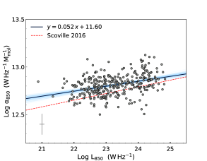
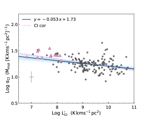
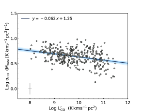
$y$ $x$ $m$ $c$ $r_{\rm s}$ $N$ Sample log $\alpha_{\rm CO}$ log $L^{\prime}_{\rm CO}$ $-0.062$ (0.009) 1.25 (0.09) $-0.33$ 335 ad log $\alpha_{850}$ log $L_{850}$ $0.052$ (0.008) 11.60 (0.18) 0.37 335 ad log $\alpha_{\rm C\,I}$ log $L^{\prime}_{\rm C\,I}$ $-0.052$ (0.013) 1.73 (0.12) $-0.3$ (0.0003) 140 Xd

The three empirical conversion factors, $\alpha_{850}$, $\alpha_{\rm C\,I}$ and $\alpha_{\rm CO}$, directly relate the observable tracer luminosity to a gas mass, according to Eqn. 1. If only one tracer ($L^{\prime}_{\rm CO}$, $L^{\prime}_{\rm C\,I}$ or $L_{850}$) is available, the empirical conversion factor we have estimated in Table LABEL:prescT is the best choice. We adopt a convention that the empirical parameters are referenced to $M_{\rm mol}$, which includes a factor 1.36 for He.

Table 10: Empirical calibration factors derived from this study. $M_{\rm mol}$ columns include a factor of 1.36 for He.

$M_{\rm H2}$ $M_{\rm mol}$ Sample $N$ $\alpha_{850}$$\,(\times 10^{12})$ $\alpha_{\rm CO}$ $\alpha_{\rm C\,I}$ $\alpha_{850}$$\,(\times 10^{12})$ $\alpha_{\rm CO}$ $\alpha_{\rm C\,I}$ $\rm{W\,Hz^{-1}\mbox{$\rm M_{\odot}$}^{-1}}$ M_⊙ (k km s^-1 pc²)^-1 $\rm{W\,Hz^{-1}\mbox{$\rm M_{\odot}$}^{-1}}$ M_⊙ (k km s^-1 pc²)^-1 daX 101 $9.9\pm 0.2$ $2.6\pm 0.1$ $12.6\pm 0.4$ $7.3\pm 0.2$ $3.5\pm 0.1$ $17.2\pm 0.5$ ad (log $L_{\rm IR}>11$) 240 $9.1\pm 0.1$ $3.1\pm 0.1$ $6.7\pm 0.1$ $4.2\pm 0.1$ ad 326 $8.8\pm 0.1$ $3.2\pm 0.1$ $6.5\pm 0.1$ $4.3\pm 0.1$ Xd 140 $9.8\pm 0.3$ $12.7\pm 0.4$ $7.2\pm 0.2$ $17.3\pm 0.5$ Xa 109 $2.5\pm 0.1$ $12.5\pm 0.3$ $3.4\pm 0.1$ $17.0\pm 0.4$

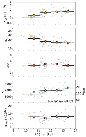
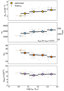
Figs 6–9 show the empirical conversion factors as a function of $L_{\rm IR}$; Fig. 10 shows the empirical conversion factors as a function of the tracer luminosity, and Fig. 11 shows their distribution when the sample is split into MS galaxies and SMGs (see Table 8 for details). All empirical factors show significant but shallow correlations with the tracer luminosity. We have carefully accounted for the co-variance between the $x$ and $y$ parameters when fitting, so the correlations we find are not caused by the involvement of $L_{850}$, $L^{\prime}_{\rm C\,I}$ and $L^{\prime}_{\rm CO}$ in the derivation of $\alpha_{850}$, $\alpha_{\rm C\,I}$ and $\alpha_{\rm CO}$. Table LABEL:calfitsT lists the fit parameters. The intrinsic scatter in all of these relationships is very small once the measurement errors are accounted for. Correlations are also seen between $L_{\rm IR}$ and $\alpha_{850}$, $\alpha_{\rm C\,I}$ and $\alpha_{\rm CO}$(Fig. 7–9), albeit with more scatter.

A correlation between $\alpha_{850}$ and $L_{850}$ was also noted by Sco16 (shown as the red dashed line on our plot) but ours is somewhat shallower ($m=0.052$ vs $m=0.07$ from Sco16), although the difference is unlikely to be significant. These shallow but significant relationships with their tracer luminosity could be further applied to give more accurate calibration (see Table LABEL:calfitsT). The trends of $\alpha_{\rm C\,I}$ and $\alpha_{\rm CO}$ with their respective tracers are explored for the first time in large numbers here.

5.2 Discussion of empirical factors relative to the literature.

5.2.1 Submillimetre dust empirical calibration, $\alpha_{850}$

The final calibration factors from this work are provided in Table LABEL:empT. A compilation of $\alpha_{850}$ values from our optimal method and those from the literature, referenced to a common $\mbox{$\alpha_{\rm CO}$}=4.3$: the Galactic value including He from Bolatto et al., 2013) is presented in Table LABEL:asublitT. Literature values cover the range, $\alpha_{850}$ = 3.6–$10.1\times 10^{12}$, comfortably within the range of estimates here: $\mbox{$\alpha_{850}$}^{\rm opt}=$ 6.5–$7.2\times 10^{12}$. The lowest value, $\mbox{$\alpha_{850}$}=3.6^{+3.6}_{-1.9}\times 10^{12}$, comes from the local sample of Orellana et al. (2017), who include H i as well as $M_{\rm mol}$ (from $L^{\prime}_{\rm CO}$). Their $\alpha_{850}$ refers to the total gas mass – sensibly, since their lower luminosity sample is more H i-dominated than the others we compare to – meaning that a lower value for $\alpha_{850}$ is required. The highest value, $\mbox{$\alpha_{850}$}=(10.1\pm 0.3)\times 10^{12}$, is from Sco16. There are two reasons why Sco16 found a significantly higher $\alpha_{850}$ compared to our analysis. The first is simple mathematics, as Sco16 quote a linear mean for a distribution that has a significant tail to higher values; in contrast, we quote a log-mean which is less sensitive to tails. This statistical bias results in a linear mean for $\alpha_{850}$ which is 20 per cent higher than the log-mean (Behroozi et al., 2013) . Assuming the shape of our $\alpha_{850}$ distribution is similar to that from Sco16, we adjust their linear mean down by 20 per cent to approximate our log-mean method. Thus our log-mean estimate of the Sco16 value is $\mbox{$\alpha_{850}$}^{\rm LM}(\rm Sco16)=8.4\times 10^{12}$. Secondly, there have been changes in the versions of the Herschel pipeline data used as the basis for the local portion of the Sco16 sample (see Appendix A). When we re-fitted the local galaxy SEDs to estimate $T_{\rm mw}$ and $L_{850}$ using the most recent Herschel flux densities (Chu et al., 2017; Clark et al., 2018) we found an increase in $L_{850}$ of $\sim 0.1$ dex compared to that reported in Sco16. Once these factors are accounted for, the Sco16 result is comparable to ours.

Table 11: Summary of our empirical dust continuum–$M_{\rm mol}$ calibration factor, $\alpha_{850}$, compared to literature values referenced to $\mbox{$\alpha_{\rm CO}$}=4.3$ (i.e. Galactic $\alpha_{\rm CO}$, including He).

.

$\alpha_{850}$($\times 10^{12}$) Sample $N_{\rm gal}$ Notes Reference W Hz^-1 M${}_{\odot}^{-1}$ $6.4\pm 0.1$ all 328 log-mean opt this work $7.2\pm 0.2$ SMGs 144 log-mean opt this work $5.9\pm 0.1$ MS 184 log-mean opt this work $10.1\pm 0.3$ local galaxies and SMGs 72 linear mean Scoville et al. (2016) 8.3 MS 30 linear mean Scoville et al. (2016) 12.7 SMGs 30 linear mean Scoville et al. (2016) $3.6^{+3.6}_{-1.9}$ local galaxies 136 median H i $+$ 4.3$L^{\prime}_{\rm CO}$ Orellana et al. (2017) $6.1\pm 0.14$ $z<0.4$ 160-$\mu$m selected 41 log-mean (ex lovales) Hughes et al. (2017) $8.4\pm 1.0$ $z=1.6$–2.9 unlensed SMGs^† 9 log-mean Kaasinen et al. (2019) $11.6\pm 1.2$ $z=1.6$–2.9 unlensed SMGs^† 9 linear mean Kaasinen et al. (2019)

Atomic carbon empirical factor: $\alpha_{\rm C\,I}$

We compare our optimised $\alpha_{\rm C\,I}$ estimates with others from the literature in Table LABEL:acilitT, and for reference we also compile the literature values for $X_{\rm C\,I}$ in Table LABEL:XCIlitT, the two are related simply by the excitation factor $Q_{10}$, as given in Eqn. 11. Our values are a weighted average of the three samples that contain C i, where we find $\langle\mbox{$\alpha_{\rm C\,I}$}\rangle=17.3\pm 0.3$ (standard error on the mean). This compares well with the only truly independent measure, $\mbox{$\alpha_{\rm C\,I}$}=21.4^{+13}_{-8}$, from absorber systems across a range of redshift by Heintz & Watson (2020), but is considerably higher than reported by many literature studies, e.g. $\mbox{$\alpha_{\rm C\,I}$}=4.9$–10.3 for a large study of (U)LIRGs by Jiao et al., 2017 and $\mbox{$\alpha_{\rm C\,I}$}=7.3^{+6.9}_{-3.6}$ for local disks by Crocker et al. (2019). Many literature studies assume a fixed value for either $X_{\rm C\,I}$ or $\alpha_{\rm CO}$ in order to derive $\alpha_{\rm C\,I}$ (typically $\mbox{$X_{\rm C\,I}$}=3\times 10^{-5}$ or $\mbox{$\alpha_{\rm CO}$}=1$ for high-$z$ SMG or local (U)LIRGs). These assumed values are very different from those we have derived here under our minimal assumption that metal rich galaxies have similar dust properties. Table LABEL:acilitT describes the assumptions made for each literature source.

The MS galaxies in this work have a value of $\alpha_{\rm C\,I}$ of $19.1\pm 0.6$, again significantly higher than that found in Crocker et al. (2019). However, J19, using a largely overlapping sample, derived a value of $\mbox{$\alpha_{\rm C\,I}$}=19.9\pm 1.9$ using the same Herschel FTS C i mapping observations. Crocker et al. use $L^{\prime}_{\rm[CO](2-1)}$ images and spatially resolved $\alpha_{\rm CO}$ estimates from Sandstrom et al. (2013), which were derived using a robust method which minimises the scatter in the gas-to-dust ratio (see also Eales et al., 2012). While there are no a priori assumptions about $\alpha_{\rm CO}$ in Crocker et al. (2019), implicit assumptions are required for the average CO $r_{21}$ excitation. The limited sensitivity of the FTS instrument to [C i](1–0) meant that C i was primarily detected in the brighter nuclear regions, where $\alpha_{\rm CO}$ tends to be lower than is typical in spiral disks ($\sim 1$ compared to $\sim 3$–4), (e.g. Sandstrom et al., 2013) – as noted by Crocker et al. Their measured $L^{\prime}_{\rm C\,I}$/$L^{\prime}_{\rm CO}$ ratios in the resolved regions are compatible with other MS galaxies in our sample (though still higher than the ratios derived for the same set of sources by J19, see Fig. 5), meaning that the $\alpha_{\rm C\,I}$/$\alpha_{\rm CO}$ ratios are also similar. As $\alpha_{\rm CO}$ in these regions is determined to be low in the Sandstrom et al. (2013) analysis, the $\alpha_{\rm C\,I}$ inferred by Crocker et al. is correspondingly lower as well.

Jiao et al. (2021) (henceforth J21) use CO(1–0), H i, [C i](1–0), dust continuum and metallicity maps to investigate the variation of $\alpha_{\rm C\,I}$ and $\alpha_{\rm CO}$ across the disks of six well-resolved local galaxies from their J19 study. They use the FIR/submm dust maps from Spitzer and Herschel and the method of Draine et al. (2007) to model the dust mass across the galaxy and relate this to a gas mass via a relationship between dust-to-gas and metallicity (Muñoz-Mateos et al., 2009; Draine et al., 2007; Sandstrom et al., 2013). As they explicitly use the dust mass together with a model of the $\delta_{\rm GDR}$ dependence on metallicity, their results are normalised to the dust properties of the Draine & Li (2007) model (hereafter DL07), which assumes $\mbox{$\delta_{\rm GDR}$}=100$ and $\mbox{$\kappa_{850}$}=0.034$ m² kg^-1 at solar metallicity. Their self-consistent DGR(ii) method derives weighted mean values of $\langle\mbox{$\alpha_{\rm C\,I}$}\rangle=19.9\pm 1.9$ (including the information from lower limits) and $\langle\mbox{$\alpha_{\rm CO}$}\rangle=2.0\pm 0.3$ ($2.6\pm 0.4$) over the same area as the C i observations (the entire CO detection region). In the central region, the $\alpha_{\rm CO}$ values are significantly lower at $\mbox{$\alpha_{\rm CO}$}^{\rm C}=1.5\pm 0.3$, while $\alpha_{\rm C\,I}$ is not found to be significantly different with $\mbox{$\alpha_{\rm C\,I}$}^{\rm C}=21.8\pm 0.5$. These values are comparable to to our average of $\mbox{$\alpha_{\rm C\,I}$}=19.1\pm 0.6$ for MS galaxies, and to the average value for $Z_{\odot}$ derived independently by Heintz & Watson (2020) of $\mbox{$\alpha_{\rm C\,I}$}(\rm HW20)=21.4^{+13.3}_{-8.2}$.

Table 12: Summary of our empirical $\alpha_{\rm C\,I}$ calibration compared to work from the literature; $\alpha_{\rm C\,I}$ is quoted including He.

.

$\alpha_{\rm C\,I}$ Sample $N_{\rm gal}$ Notes Reference M_⊙ (k km s^-1 pc²)^-1 $17.0\pm 0.3$ log $L_{\rm IR}>11$ weighted average this work $19.1\pm 0.6$ MS weighted average this work $16.2\pm 0.4$ SMGs weighted average this work $10.3\pm 0.3$ (U)LIRGs 71 assuming $\mbox{$X_{\rm C\,I}$}=3\times 10^{-5}$ Jiao et al. (2017) $4.9\pm 0.3$ (U)LIRGs 71 CO(1–0) with $\mbox{$\alpha_{\rm CO}$}=1.1$ Jiao et al. (2017) $7.3^{+6.9}_{-3.6}$ resolved local disks 18 CO(2–1) and resolved $\alpha_{\rm CO}$ from S13 Crocker et al. (2019) $19.9\pm 1.9$ resolved local disks 6 H i, CO(1–0), C i, dust, $Z$ ($\kappa_{\rm eff}\sim 1300$) Jiao et al. (2021) $16.2\pm 7.9$ $z=3$ lensed SMGs 16 multi-$J$ CO, C i  dust modelling Harrington et al. (2021) $21.4^{+13.3}_{-8.2}$ GRB/QSO absorbers 19 $H_{2}$ and C i absorption lines at $\rm{Z_{\odot}}$ Heintz & Watson (2020) 17.6 theory for $\mbox{$\zeta_{\rm CR}$}=5\times 10^{-17}\rm{s^{-1}}$ Offner et al. (2014)

Table 13: Summary of our $X_{\rm C\,I}$ calibrations compared to other work in the literature.

$X_{\rm C\,I}$($\times 10^{-5}$) Sample $N_{\rm gal}$ Notes Reference $1.6^{+0.5}_{-0.4}$ $z=0$–5 log $L_{\rm IR}>11$ 90 $L_{850}$, CO, C i with $\mbox{$\kappa_{\rm H}$}^{\rm N}=1884$ kg m^-2 this work $2.5\pm 1.0$ local SF 11 CO(1–0) and $\mbox{$\alpha_{\rm CO}$}=1$ Jiao et al. (2019) $1.3\pm$ local SF 9 CO(1–0) and $\alpha_{\rm CO}$ from S13 Jiao et al. (2019) $1.6\pm 0.7$ $z\sim 1.2$ MS 11 CO(2–1) and $\alpha_{\rm CO}$(Z) ($\langle\mbox{$\alpha_{\rm CO}$}\rangle=3$) Valentino et al. (2018)^† $2.0\pm 0.5$ $z\sim 1.2$ MS 11 dust and $\delta_{\rm GDR}$(Z) ($\langle\mbox{$\delta_{\rm GDR}$}\rangle=134$) Valentino et al. (2018)^† $3.9\pm 0.4$ $z=2-3$ SMGs 14 CO(4–3), CO(1–0) and $\mbox{$\alpha_{\rm CO}$}=1$ Alaghband-Zadeh et al. (2013)^† $8.4\pm 3.5$ SMGs/QSOs 10 CO(3–2) and $\mbox{$\alpha_{\rm CO}$}=0.8$ Walter et al. (2011) $8.3\pm 3.0$ local (U)LIRGS 23 CO(1–0) and $\mbox{$\alpha_{\rm CO}$}=0.8$ Jiao et al. (2017); Jiao et al. (2019)^† $0.9\pm 0.3$ $z=1$ ISM selected 2 CO(2–1), C i and $\mbox{$\alpha_{\rm CO}$}=2.6$ Boogaard et al. (2020) $2.0\pm 0.4$ $z=1$ ISM selected 3 1.2 mm, C i and $\mbox{$\alpha_{850}$}=6.7\times 10^{12}$ from Sco16 Boogaard et al. (2020) ${}^{\ast}1.6^{+1.3}_{-0.7}$ $z=2$–4 GRB/QSO absorbers 19 H₂ and $\rm{C^{0}}$ absorption lines for $\rm{Z_{\odot}}$ Heintz & Watson (2020) ${}^{\ast}7^{+7}_{-3.5}$ NGC 7469 (CND) 1 AGN, dynamical mass, $L^{\prime}_{\rm C\,I}$ and $L^{\prime}_{\rm CO}$ Izumi et al. (2020) ${}^{\ast}1.4-5$ NGC 6240 1 $\alpha_{\rm CO}$ from CO–SLED, high-density tracers Cicone et al. (2018) and two-phase LVG modelling Papadopoulos et al. (2014)

CO empirical factor: $\alpha_{\rm CO}$

We compare our optimised $\alpha_{\rm CO}$ estimates with others from the literature in Table LABEL:acolitT. Sophisticated LVG modelling with very large datasets which include high-density gas tracers, optically thin CO isotopologues, full CO SLEDs, and sometimes the C i lines and dust emission (e.g. Weiß et al., 2007; Papadopoulos et al., 2012b; Papadopoulos et al., 2014; Israel, 2020; Harrington et al., 2021) can break some of the model degeneracies of the optically thick CO lines, though the method is still reliant on assumptions for [CO/H₂], isotopologue ratios, the number of components allowed (single components give very different results to multiple components) and the allowed range of velocity gradients in the models.

The best examples are NGC 6240 (Papadopoulos et al., 2014) and the Planck lensed galaxies (Harrington et al., 2021) where detailed LVG modelling and comprehensive datasets have sufficient constraints to break the degeneracies which usually be-devil this method. The two-component LVG result for NGC 6240 is $\mbox{$\alpha_{\rm CO}$}=2$–4 (Papadopoulos et al., 2014) (cf. $\alpha_{\rm CO}$=0.6 when using a single component LVG model Papadopoulos et al., 2012b) and we can further use the ratio of $\mbox{$L^{\prime}_{\rm C\,I}$}/\mbox{$L^{\prime}_{\rm CO}$}$ measured by Cicone et al. (2018) and our relationship, $\mbox{$L^{\prime}_{\rm C\,I}$}/\mbox{$L^{\prime}_{\rm CO}$}=\mbox{$\alpha_{\rm CO}$}/\mbox{$\alpha_{\rm C\,I}$}=3324\,\mbox{$\alpha_{\rm CO}$}\mbox{$X_{\rm C\,I}$}$, to infer that $\mbox{$X_{\rm C\,I}$}=1.4$–$2.9\times 10^{-5}$ in the starburst region. In fact, our optimised values for this galaxy using global fluxes, are $\mbox{$\alpha_{\rm CO}$}({\rm daX})=2.9\pm 0.6$, $\mbox{$X_{\rm C\,I}$}({\rm daX})=(2.4\pm 0.5)\times 10^{-5}$, $\mbox{$\kappa_{\rm H}$}({\rm daX})=2800\pm 700$ ($\mbox{$\delta_{\rm GDR}$}=200$), in excellent agreement. The Planck lensed galaxies analysed by Harrington et al. (2021) do not have the same degeneracy-breaking lines used by (Papadopoulos et al., 2014) in their analysis, but they do have multi-$J$ CO coverage and incorporate the C i lines and the dust continuum emission in their model fitting, based on Weiß et al. (2007). They assume similar dust parameters as we do for their normalisations ($\mbox{$\delta_{\rm GDR}$}=120$–150 with $\mbox{$\kappa_{850}$}=0.08$ m² kg^-1). With this, they infer an average $\mbox{$\alpha_{\rm CO}$}=3$–4 and an average $\mbox{$\alpha_{\rm C\,I}$}=16.2\pm 7.9$ (incl. He), remarkably consistent with our results, given our very simple approach.

Table 14: Summary of our empirical $\alpha_{\rm CO}$ calibrations compared to work in the literature, $\alpha_{\rm CO}$ is quoted including a factor of 1.36 for He.

$\alpha_{\rm CO}$ Sample $N_{\rm gal}$ Notes Reference M_⊙ (k km s^-1 pc²)^-1 $3.6^{+1.3}_{-1.0}$ $z=0$–5, log $L_{\rm IR}>11$ 90 $L_{850}$, CO, C i with $\mbox{$\kappa_{\rm H}$}^{\rm N}=1884$ kg m^-2 this work $4.2^{+1.8}_{-1.1}$ $z=0$–5, log $L_{\rm IR}>11$ 240 $L_{850}$, CO with $\mbox{$\kappa_{\rm H}$}^{\rm N}=1884\,\mbox{kg\,m${}^{-2}$}$ this work $4.8^{+1.3}_{-1.1}$ local MS, log $L_{\rm IR}<11$ 88 $L_{850}$, CO with $\mbox{$\kappa_{\rm H}$}^{\rm N}=1884$ kg m^-2 this work ${}^{\ast}3.1^{+3.1}_{-1.5}$ local disks 26 CO(2–1), $r_{21}=0.7$, H i, dust Sandstrom et al. (2013) ${}^{\ast}4.2$ (3.5–5.4) MW large scale $\gamma$-ray various Remy et al. (2017) ${}^{\ast}3.4\pm 2.1$ Planck lensed SMGs 24 LVG: multi-$J$ CO, C i and dust Harrington et al. (2021) ${}^{\ast}4.1^{+4}_{-2}$ NGC 7469 (CND) 1 AGN, dynamical mass, $L^{\prime}_{\rm CO}$ Izumi et al. (2020) ${}^{\ast}2-4$ NGC 6240 1 LVG: multi-$J$ CO, dense gas tracers Papadopoulos et al. (2014) ${}^{\ast}3.8^{+1.0}_{-0.7}$ $z=0$–5 22 CO, C i, Z and absorber based $\alpha_{\rm C\,I}$ Heintz & Watson (2020) ${}^{\ast}4.4^{+2.0}_{-1.4}$ local galaxies 24 C ii, CO(1–0) and modelling at $\rm{Z_{\odot}}$ Accurso et al. (2017) ${}^{\ast}0.6\pm 0.2$ (U)LIRGs 28 LVG: Single component, multi-$J$ CO Papadopoulos et al. (2012b) ${}^{\ast}2-6$ (U)LIRGs 28 LVG: Two-comp, free d$V$/d$R$, dense-gas tracers Papadopoulos et al. (2012b) ${}^{\ast}3.9\pm 1.1$ local disks 9 CO(1–0), H i, dust Eales et al. (2012) $1.8\pm 0.5$ MW local clouds 6 H i, CO(1–0), $\gamma$-ray Remy et al. (2017) $2.9\pm 0.5$ MW local clouds 6 H i, CO(1–0), 850-$\mu$m dust Remy et al. (2017) 2.9 Taurus 1 H i, CO(1–0) and extinction/reddening Chen et al. (2015) $2.4\pm 0.4$ local disks 7 CO(1–0), H i, dust Cormier et al. (2018) $1.9\pm 0.3$ resolved local disks 6 H i, CO(1–0), [C i](1–0), dust, $Z$, $\kappa_{\rm eff}\sim 1300$ Jiao et al. (2021) $3.2\pm 1.0$ $z=4$ lensed SMGs 9 CO(2–1), [C i](1–0) $\mbox{$X_{\rm C\,I}$}=3\times 10^{-5}$ Bothwell et al. (2017)

5.3 Lack of bi-modality in the conversion factors

Our sample contains normal star forming galaxies – those obeying the SFR–$M_{\star}$ correlation that forms as a result of the more intimate relationship between SFR and H₂ – as well as many extreme star-forming systems, which belong to the (U)LIRG and high-$z$ submillimeter selected samples. Here we remind the reader that we refer to the extreme SF group – those that supposedly require a lower $\alpha_{\rm CO}$ – as ‘SMGs’, and the normal star forming sources as ‘MS galaxies’, or sometimes just ‘MS’. As mentioned in Section 2, the assignment of the galaxies to either category is by nature of the data rather ‘fuzzy’ as we do not have a measure of SFR or stellar mass for all sources, nor any homogeneous way to estimate them. We thus rely on the categories used by previous authors where possible, especially for high-$z$ sources. The $z=1$ galaxies from the samples of Bourne et al. (2019); Valentino et al. (2018, 2020) are deemed to be ‘MS’, as are the sources from ASPECs (Boogaard et al., 2020). Most low redshift sources with log $L_{\rm IR}$<12 are classed as ‘MS’ though there are some exceptional LIRG class sources in the local Universe which have extreme properties as evidenced by their FIR, MIR lines and vibrational HCN (Díaz-Santos et al., 2017; Falstad et al., 2021). We note that using a more conservative separation when assigning galaxies into MS and extreme starburst categories does not change any of the results. We therefore conclude that while our assignment of sources into the two SF categories is not perfect, this categorisation is not capable of masking any strong bi-modality in the observable ratios.

Fig. 11 and Table 8 detail the distributions of conversion factors for each sample, split into MS galaxies and SMGs. While formally there are significant differences in the parameters for some samples, these are very small – around 10–20 per cent in the mean, rather than the factor $\sim 3$–$4\times$ often assumed for $\alpha_{\rm CO}$ (e.g. Downes & Solomon, 1998, $\alpha_{\rm CO}$=0.8, derived for four ULIRGs). In fact, only the ad sample shows any difference in $\alpha_{\rm CO}$ between the MS galaxies and SMGs, while the estimates based on C i and CO, or on all three tracers, show no significant difference. This is partially explained by the larger luminosity range in the ad sample, combined with the previously noted negative correlation between $\alpha_{\rm CO}$ and luminosity (Figs 9 and 10), with a factor $\sim 2\times$ reduction in $\alpha_{\rm CO}$ for a factor $\sim 100\times$ increase in $L^{\prime}_{\rm CO}$. We cannot rule out that the correlation of $\alpha_{\rm CO}$ with luminosity is the true reason that the ad sample shows a significant difference between MS galaxies and SMGs.

This is not the first time that lack of bi-modality in $\alpha_{\rm CO}$ has been reported when compared to dust-based determinations (e.g. Magdis et al., 2012; Rowlands et al., 2014; Genzel et al., 2015). The range of $\alpha_{\rm CO}$ we find for SMGs (see Fig. 9) is well within the framework set out by Papadopoulos et al. (2012a), who noted that galaxies with a highly turbulent ISM (e.g. ULIRGs and SMGs) can have $\alpha_{\rm CO}$ similar to galaxies with a much more quiescent ISM, the only difference being that in a turbulent ISM, the distribution of gas mass as a function of density is weighted to higher densities than in a less-turbulent ISM.

Recent joint SLED/SED modelling of an exquisite dataset that includes CO, C i and dust continuum for lensed SMGs (Harrington et al., 2021) finds a mean $\mbox{$\alpha_{\rm CO}$}=3.4$–4.2 for these highly turbulent galaxies (albeit with a large dispersion). The Harrington et al. radiative transfer models employ a continuum distribution of molecular gas mass as a function of average Mach number (and average density of the molecular cloud ensemble), making them better equipped to ‘capture’ any re-distribution of the underlying molecular gas mass towards higher densities. While important for other issues (e.g. the initial conditions of star formation in SMGs/ULIRGs), such a re-distribution in a highly turbulent ISM may actually leave $\alpha_{\rm CO}$ statistically unaffected. The initial reports of a bimodal $\alpha_{\rm CO}$ factor in the local Universe, with $\sim$4-5$\times$ lower values for ULIRGs than LIRGs and ordinary spirals, can possibly be explained by a CO-luminous, strongly unbound, low-density molecular gas component found preferentially in ULIRGs. Such a component can dominate the global CO(1–0) line luminosities of ULIRGs/SMGs (even if containing only small fractions of their total molecular gas), while its large $\rm K_{vir}$ values will yield systematically low $\alpha_{\rm CO}$ factors, under one-component LVG modelling (Equation 9).

For individual galaxies, only multi-component models of SLED/SED (that also include molecules/transitions tracing the dense gas) can properly account for this effect (e.g. Papadopoulos et al., 2014; Harrington et al., 2021), while for large galaxy samples, our cross-calibration of $\alpha_{\rm CO}$ against the other two molecular gas mass tracers, is the most economical method. In that regard it is worth noting that dust continuum is immune to the gas-dynamics effects described above, i.e. a diffuse low-density, unbound, $\rm H_{2}$ gas component will contribute very little to the total dust continuum if its gas/dust mass is indeed low. The optically thin C i line emission will also be much less sensitive than CO(1–0) to such gas-dynamics effects exactly because of its low optical depths. These are perhaps the reasons why our cross-calibration of $\alpha_{\rm CO}$ against dust and C i emission has not uncovered any obvious bimodality of its values in MS galaxies compared to SMGs.

The range of values we find for $\alpha_{\rm CO}$ is consistent with expected values for $Z>0.5\,Z_{\odot}$ galaxies (Accurso et al. 2017, based on calibrating $\alpha_{\rm CO}$ using Cii). Using their predictions, we would expect $2.7<\mbox{$\alpha_{\rm CO}$}<15.2$ for the likely range of metallicity and offset from the MS in our sample.

Figure 12: Results assuming a bi-modal behaviour for $\alpha_{\rm CO}$. We run the optimisation process with the normalisation for SMGs set to $\mbox{$\alpha_{\rm CO}$}^{\rm N}(\rm SMG)=0.8$, keeping MS galaxies at $\mbox{$\kappa_{\rm H}$}^{\rm N}(\rm MS)=1884$ kg m^-2(equivalent to $\alpha_{\rm CO}$=2.8). This creates the strong bi-modality in $\alpha_{\rm CO}$ but also induces a similarly strong or even stronger effect in $\kappa_{\rm H}$ and $X_{\rm C\,I}$, which would be mirrored in $\alpha_{850}$ and $\alpha_{\rm C\,I}$.

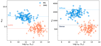
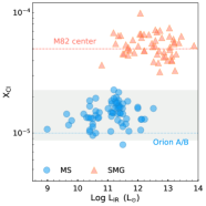
Our underlying assumption: that the dust–gas properties of MS galaxies and SMGs can be described as a uni-modal distribution with well defined mean and scatter, is based on our finding that the luminosity ratios (Fig. 2) – the most basic observables used in deriving the empirical conversion factors – have such a distribution. They show no evidence for the strong bi-modality advocated for $\alpha_{\rm CO}$ in some of the literature. That the distribution of the observed luminosity ratio is, to first order, similar to the distribution of the conversion parameters, is the simplest ‘Occam’s Razor’ assumption we can make.

To see what a different initial assumption would mean for the conversion factors, we repeated our analysis, this time inserting the popular bi-modal behaviour in $\alpha_{\rm CO}$ (Greve et al., 2005; Weiß et al., 2005; Tacconi et al., 2006, 2008; Genzel et al., 2010; Walter et al., 2011; Alaghband-Zadeh et al., 2013; Jiao et al., 2017; Valentino et al., 2018) as our prior, such that the sample mean normalisations for SMGs and MS galaxies are set to be different: $\mbox{$\alpha_{\rm CO}$}^{\rm N}(\rm SMG)=0.8$ and $\mbox{$\kappa_{\rm H}$}^{\rm N}(\rm MS)=1884$ kg m^-2. Our optimal method then allows the data to return the most likely values for the other parameters under these assumptions.

Fig. 12 shows the results with this bi-modal normalisation, (blue points: MS galaxies, red points: SMGs). By design, we have reproduced the extreme bi-modality $\mbox{$\alpha_{\rm CO}$}(\rm MS)\sim 3$–4 and $\mbox{$\alpha_{\rm CO}$}(\rm SMG)\sim 1$, but Fig. 12 clearly shows that the same extreme bi-modality has to be present in $\kappa_{\rm H}$  ($\delta_{\rm GDR}$) and $X_{\rm C\,I}$, giving a clear prediction that $\mbox{$X_{\rm C\,I}$}(\rm SMG)\geq 4\times 10^{-5}$ if the bimodality in $\alpha_{\rm CO}$ really exists, with essentially no overlap in $X_{\rm C\,I}$ between the MS galaxies and SMGs. To test this will require an independent determination of $X_{\rm C\,I}$ in SMGs, without reference to dust or CO calibration. To date, there is no such determination of $X_{\rm C\,I}$, although Izumi et al. (2020) observed the nearby LIRG NGC 7469 with ALMA, using kinematic data to derive $\rm{M_{dyn}}$, which is the sum of $M_{\rm H2}$, stellar mass and dark matter. This method has promise, but the systematic uncertainties in $M_{\rm H2}$ from this analysis are too large (0.3 dex) to answer our question. While the Izumi et al. study clearly indicates that the [$\rm{C^{0}}/CO$] abundance can be enhanced in extreme environments, the CND is only a tiny region and the global ratio for this source is very similar to other LIRGs, with $\mbox{$L^{\prime}_{\rm C\,I}$}/\mbox{$L^{\prime}_{\rm CO}$}=0.20\pm 0.04$. Any study which wishes to test the bi-modality hypothesis must also be representative of the galaxy global properties.

Here we must stress again that for individual galaxies, joint SLED/SED radiative transfer models of well-sampled SLEDs and dust emission SEDs do recover Galactic-valued $\alpha_{\rm CO}$  factors even in (U)LIRGs or SMGs (Papadopoulos et al., 2014; Harrington et al., 2021). However such results cannot be used in a statistical sense, i.e. as typical of the respective galaxy populations for obvious reasons, and our statistical approach remains the sole avenue.

Indeed, the only way that a bi-modal $\alpha_{\rm CO}$ for MS galaxies and SMGs can be reconciled with $M_{\rm H2}$ estimates using dust or C i is to impose the same bi-modality on their conversion parameters ($\kappa_{\rm H}$, $X_{\rm C\,I}$, $\alpha_{850}$, $\alpha_{\rm C\,I}$). A reduction of $\alpha_{\rm CO}$ by a factor $3\times$ necessitates a decrease [increase] in $\kappa_{\rm H}$ [$X_{\rm C\,I}$] by the same factor. Thus, if $\mbox{$\alpha_{\rm CO}$}=0.8$ is preferred for extreme star-forming galaxies (e.g. Walter et al., 2011), then $\mbox{$\kappa_{\rm H}$}=600$ ($\mbox{$\delta_{\rm GDR}$}=43$ for $\mbox{$\kappa_{850}$}=0.071$ m² kg^-1) and $\mbox{$X_{\rm C\,I}$}=5.3\times 10^{-5}$ must also be adopted (statistically, for this galaxy population). This discrepancy was previously noted by Bothwell et al. (2017) and Valentino et al. (2018) who found that using $\mbox{$X_{\rm C\,I}$}(\rm SMG)=3\times 10^{-5}$ with $L^{\prime}_{\rm C\,I}$ as a tracer resulted in larger gas masses than using $L^{\prime}_{\rm CO}$ with the ‘ULIRG’ value of $\mbox{$\alpha_{\rm CO}$}=0.8$. Therefore, the popular ‘choices’ of $\mbox{$\alpha_{\rm CO}$}=0.8$ and $\mbox{$X_{\rm C\,I}$}=3\times 10^{-5}$ are incompatible with each other.

Based on our current understanding, there are two plausible physical mechanisms which may cause an increase in $X_{\rm C\,I}$ and a decrease in $\kappa_{\rm H}$ in extreme ISM conditions. The effect of enhanced cosmic ray densities on carbon chemistry (Bisbas et al., 2015, 2021; Glover & Clark, 2016; Gong et al., 2020) favour a higher $\rm[C^{0}/CO]$ abundance, however, this mechanism is density dependent and is less effective in dense regions, which typify the ISM of SMGs. Thus while extreme environments with elevated cosmic rays or X-rays would certainly act to increase $X_{\rm C\,I}$ at a fixed density, it does not simply follow that extreme SF activity will produce high $X_{\rm C\,I}$ since those same regions (CRDR/XDR) are typically found in regions with increased density.

The higher dense gas fractions common in SMGs may favour higher rates of grain growth, or mantling, both of which would reduce the value of $\kappa_{\rm H}$ – i) by decreasing the $\delta_{\rm GDR}$ and ii) by increasing the dust emissivity, $\kappa_{850}$. Our results imply, however, that any such changes must act in harmony with each other so as to maintain the same observable ratios, so an increase in $X_{\rm C\,I}$ must correlate directly with a decrease in $\kappa_{\rm H}$ and $\alpha_{\rm CO}$. This prediction is a clear challenge to models, and full astro-chemical simulations for the extreme physical conditions expected in the ISM of SMGs and ULIRGs will be needed to explore how the three tracers can vary in the exact same way through very different physical mechanisms.

5.4 On the robustness of our choices

5.4.1 Impact of uncorrected $f_{\rm H\,I}$>1 galaxies

Statistically, the effect of having uncorrected $f_{\rm H\,I}$>1 galaxies is small, since there are only 15 such galaxies, where $\langle\mbox{$\alpha_{\rm CO}$}\rangle$ increases by +0.27 in their luminosity bin compared to when they are removed altogether (by +0.18 compared to when they have been corrected). We are thus confident that dust associated with H i is not biasing our overall determination of conversion factors and their trends, at least in this sample. For individual galaxies, however, the difference in $\alpha_{\rm CO}$ can be very large. When using this method for low-redshift galaxies with significant H i within the dust-emitting region, corrections are needed.

5.4.2 Impact of using a constant $T_{\rm mw}$

The strong correlation found between $T_{\rm mw}$ and luminosity (Fig. 1) has not been considered in previous works. In Appendix H.2, we show a comparison of results using our empirical $T_{\rm mw}$ relations to those for constant, $T_{\rm mw}$=25 k. Summarising these findings:

1. The median offsets between parameters when using constant vs. variable $T_{\rm mw}$ are $<0.015$ dex. The scatter in a parameter is generally within 0.1 dex (Fig. 16). Thus the global averages we present in this paper are not affected by a change to constant $T_{\rm mw}$=25 k.

2. Allowing $T_{\rm mw}$ to vary with $L_{\rm IR}$ is more realistic and leads to a shallow but significant trend with luminosity, such that $\alpha_{\rm CO}$ decreases with increasing $L_{\rm IR}$, while $\kappa_{\rm H}$, $\alpha_{850}$ and $X_{\rm C\,I}$ increase slightly. Using a constant $T_{\rm mw}$ of 25 k produces no trends of any conversion factor with $L_{\rm IR}$ (Fig. 17).

3. Using a constant $T_{\rm mw}$ of 25 k results in gas masses up to 0.1 dex lower at log $L_{\rm IR}<11$ and 0.1 dex higher at $l_{\rm IR}<12.0$ compared to the variable $T_{\rm mw}$ used in the main analysis (Fig. 18).

6 Discussion

The diverse galaxies in this study show a remarkable consistency in their gas mass tracers, with linear relationships between all three pairs of observables, $L_{850}$, $L^{\prime}_{\rm C\,I}$ and $L^{\prime}_{\rm CO}$.

We find weak trends in the conversion factors with $L_{\rm IR}$; decreasing $\alpha_{\rm CO}$, $\alpha_{\rm C\,I}$ and increasing $\alpha_{850}$, $\kappa_{\rm H}$, $X_{\rm C\,I}$. These trends are very shallow, amounting to a factor $<2\times$ change over 2–3 orders of magnitude in luminosity. The intrinsic variation in $\kappa_{\rm H}$ and $X_{\rm C\,I}$ (the physical quantities encompassing most of the uncertainties in the corresponding conversion factors) is likely very small, and approximating them with a single constant value should be robust. For the sub-samples with a C i tracer (daX, Xa, Xd), we see decreases in all three tracer conversion factors at log $L_{\rm IR}<11$: $X_{\rm C\,I}$ (15–25 per cent), $\alpha_{\rm CO}$ (10–30 per cent) and $\kappa_{\rm H}$ ($\delta_{\rm GDR}$: 20–25 per cent). However, the data indicating a drop in conversion factors originates from the J19 sample (see earlier discussions). More C i studies of normal star-forming galaxies in the local Universe are urgently required to further explore any such trend, in particular using the global C i line emission, rather than that of the central few kpc of a galaxy.

The average values of $X_{\rm C\,I}$, $\alpha_{\rm CO}$ and $\kappa_{\rm H}$ ($\delta_{\rm GDR}$) for galaxies with all three tracers (the daX sample) and log $L_{\rm IR}>11$ are our ‘reference’ values, $\mbox{$\alpha^{\rm R}_{\rm CO}$}=3.7$ (including He), $\mbox{$X^{\rm R}_{\rm C\,I}$}=1.6\times 10^{-5}$, $\mbox{$\kappa_{\rm H}$}^{\rm R}=1990\,(\mbox{$\delta^{\rm R}_{\rm GDR}$}=141)$. These agree within the errors with the mean values determined using only two tracers. These reference values are not unique because only the ratios and products of the conversion factors are constrained by the observables, $L^{\prime}_{\rm C\,I}$/$L^{\prime}_{\rm CO}$, $L^{\prime}_{\rm C\,I}$/$L_{850}$ and $L_{850}$/$L^{\prime}_{\rm CO}$.

Once a conversion factor is known or assumed, however, the others can be determined by the self-consistent ratios listed in Table 3. For example, using the ad sub-sample and normalising to $\mbox{$\kappa_{\rm H}$}^{\rm N}=2800\,\rm m^{2}\,kg^{-1}$ would produce $\mbox{$X_{\rm C\,I}$}=1.1\times 10^{-5}$ and $\mbox{$\alpha_{\rm CO}$}=4.7$, in reasonable agreement with Accurso et al. (2017) for $Z=0.6\,Z_{\odot}$, while normalising to $\mbox{$\alpha_{\rm CO}$}^{\rm N}=0.8$ gives $\mbox{$X_{\rm C\,I}$}=5.8\times 10^{-5}$ and $\mbox{$\delta_{\rm GDR}$}=34$. While the data are consistent with both of these possibilities, or any other combination of the above ratios, we must caution that the low values of $\alpha_{\rm CO}$  often recovered from CO-only methods (and after modeling only a few low-J CO lines) may be an artifact of well-known gas-dynamics effects, which are expected to have very little impact on the global C i line emission and none whatsoever on the corresponding dust continuum.

For galaxies at log $L_{\rm IR}<11$ we can only use the ad sample (CO and dust continuum) because of the uncertainties surrounding the C i^cor galaxies. For the 88 galaxies at log $L_{\rm IR}<11$ with CO and dust measurements, $\mbox{$\alpha_{\rm CO}$}=4.8^{+1.4}_{-1.1}$ (including He), with $\langle\mbox{$\kappa_{\rm H}$}\rangle=1718$ kg m^-2($\delta_{\rm GDR}$=122) but note that this is still a sample of massive and metal-rich galaxies, just at lower log $L_{\rm IR}\sim 9-11$. This study is not applicable to low mass metal-poor galaxies.

7 Conclusions

We have cross-calibrated the three mainstays of molecular gas measurements in extra-galactic astronomy: ¹²CO(1–0), [C i](${}^{3}P_{1}$–${}^{3}P_{0}$) and submm continuum emission from dust. This analysis uses galaxy samples spanning $0<z<5$ and more than four orders of magnitude in $L_{\rm IR}$. All the galaxies are metal rich and/or massive, to remove the need for large corrections for metallicity effects.

• We present a new method of optimising gas mass estimation when multiple tracers are observed, making use of the intrinsic scatter in all three pairs of gas tracers. We demonstrate its effectiveness compared to the simpler method used previously in the literature, and give examples and prescriptions for its use.

• In a purely empirical analysis, we show that $L^{\prime}_{\rm C\,I}$ is the molecular gas tracer with the least intrinsic scatter, particularly at log $L_{\rm IR}>11$. In such galaxies, $L^{\prime}_{\rm C\,I}$ should be the preferred tracer, all other considerations being equal.

• Using our optimised method, we determine the mean empirical conversion factors for $M_{\rm mol}$ (including He). For log $L_{\rm IR}>11$ these are: ${\mbox{$\alpha_{\rm C\,I}$}^{\rm R}=17.0\pm 0.3}$, $\mbox{$\alpha_{850}$}^{\rm R}=(6.9\pm 0.1)\times 10^{12}$, $\mbox{$\alpha_{\rm CO}$}^{\rm R}=4.0\pm 0.1$, with a scatter of 0.11-0.15 dex. These values are for an overall normalisation set to the average dust properties of local galaxies and diffuse dust in the Milky Way ($\kappa_{\rm H}$= $\delta_{\rm GDR}$/ $\kappa_{850}$= 1884 kg $\rm m^{-2}$). A change in this choice of normalisation will affect $\alpha_{\rm CO}$ and $\alpha_{\rm C\,I}$ in a proportional manner and $\alpha_{850}$ in an inversely proportional way. Our reference conversion values can be applied to any metal-rich galaxy with $Z>0.5\,Z_{\odot}$ in the range $0<z<6$.

• Using the same method we determine the principal mean physical parameters on which these conversion values depend. For galaxies at log $L_{\rm IR}>11$: ${\mbox{$X_{\rm C\,I}$}^{\rm R}=1.6\times 10^{-5}}$, $\mbox{$\kappa_{\rm H}$}^{\rm R}=1990\,(\mbox{$\delta_{\rm GDR}$}^{\rm R}=141)$.

• The relationships between the observables, $L_{850}$, $L^{\prime}_{\rm CO}$ and $L^{\prime}_{\rm C\,I}$ are consistent with being linear and the ratios of these observables do not show a strong dependence on IR luminosity, dust temperature, redshift or the intensity of star formation.

• The ratio of $L^{\prime}_{\rm C\,I}$/$L^{\prime}_{\rm CO}$ is marginally (3$\sigma$) different for MS galaxies and SMGs, with the latter having higher $L^{\prime}_{\rm C\,I}$/$L^{\prime}_{\rm CO}$, broadly consistent with expectations from astro-chemical cloud models that include enhanced cosmic rays.

• We find $\mbox{$Q_{10}$}=0.48$ to be a reasonable choice for the excitation function (required to convert $L^{\prime}_{\rm C\,I}$ to $M_{\rm C\,I}$), based on recent analysis showing that $Q_{10}$ has a super-thermal behaviour in non-LTE conditions (Papadopoulos et al., 2022). For a range of plausible galaxy ISM density and gas temperatures, the 99th percentile confidence interval on this value is $\pm 16$ per cent.

• We present empirical relations for the mass-weighted dust temperature, $T_{\rm mw}$, to allow observers to better estimate their dust calibration factors. We find a significant trend, where $T_{\rm mw}$ increases with $L_{\rm IR}$. The median $T_{\rm mw}$ for SMGs at $z\sim 2.5$ is $\mbox{$T_{\rm mw}$}^{\rm SMG}=30.1\pm 0.7$ k, while for MS galaxies $\mbox{$T_{\rm mw}$}^{\rm\rm MS}=23.0\pm 0.4$ k.

• We find a weak trend for $\kappa_{\rm H}$ and $X_{\rm C\,I}$ to increase with $L_{\rm IR}$, and a similar trend for $\alpha_{\rm CO}$ to decrease. The empirical conversion factors ($\alpha_{\rm CO}$, $\alpha_{\rm C\,I}$ and $\alpha_{850}$) also show a shallow but significant correlation with their tracer luminosities. These trends are not apparent if a constant $T_{\rm mw}$ is adopted. They are therefore driven by the change in $T_{\rm mw}$ with luminosity.

• Using an Occam’s Razor assumption that metal-rich galaxies have similar dust emissivity per unit gas mass, we find no evidence for the factor 3–4 $\alpha_{\rm CO}$ bi-modality between SMGs and MS galaxies often adopted in the literature. The shallow trends we do find reflect the common assumption that extreme SF systems have lower $\alpha_{\rm CO}$ and higher $X_{\rm C\,I}$, albeit at a far more subtle level, with only a $\sim 15$ per cent difference in the sample mean $\alpha_{850}$ (higher), $\alpha_{\rm C\,I}$ (lower) and $\alpha_{\rm CO}$ (lower) for extreme star-forming galaxies versus ‘normal’ MS star-formers. o overall

• With the Occam’s Razor assumption, we also find no evidence to support the extremely high global estimates of $X_{\rm C\,I}$ ($\sim 6\times 10^{-5}$) reported in some literature for ULIRGs/SMGs – the high reported values are a consequence of assuming a low $\mbox{$\alpha_{\rm CO}$}\sim 1$. High $X_{\rm C\,I}$ values may be expected, and indeed have been measured in small ($<500$pc) regions such as M82 (nuclear starbursts) and XDR regions around AGN, but the extent to which a global estimate would be enhanced depends on the dominance of that extreme environment in the galaxy’s H₂ reservoir.

• One can, however, still postulate a different prior for the normalisation assumption and impose the popular bimodality in $\alpha_{\rm CO}$. The constancy of the measured tracer luminosity ratios then forces the conversion factors for the other two tracers (dust and C i) to become bi-modal in the same way.

We conclude by noting that lacking a direct $M_{\rm H2}$  measurement method (i.e. via the $\rm H_{2}$ lines themselves), one must assume a normalisation for one of the sample mean conversion factors in statistical studies like ours. In the present study we choose to benchmark to the dust emission, with $\mbox{$\kappa_{\rm H}$}^{\rm N}=1884$ kg m^-2. Other normalisation choices can of course be made, but currently dust emission is the simplest and best understood tracer, and has the advantage of being totally insensitive to the gas-dynamic effects that affect the $\alpha_{\rm CO}$ conversion factor (e.g. unbound molecular gas components in the winds that exist in actively star-forming galaxies; winds which can be CO-bright while carrying little mass). The [C i](1–0) line emission will also be largely unaffected by these gas-dynamics effects, and as such the corresponding conversion factor, $\alpha_{\rm C\,I}$, shows promise as a good benchmark, borne out by the empirical finding that it has the least intrinsic scatter of the three tracers. With more extensive observational and theoretical studies of C i line emission (particularly in galaxies of lower IR luminosity), the limits of its usefulness as a gas tracer can be determined.

Data Availability

Data tables based on the samples used in this paper are available via anonymous ftp to cdsarc.ustrasbg.fr (130.79.128.5), alternatively via http://cdsarc.u-strasbg.fr/viz-bin/qcat?J/MNRAS/. The datasets were derived from sources in the public domain, which are listed in Table 1.

Appendix A Notes on the literature fluxes

In order to produce a homogeneous and up-to-date set of fluxes, we have applied the following corrections.

Corrections to previously published work:

1. Since Sco16 was published, the 500-$\mu$m flux densities used for their local sample (Dale et al., 2012) were updated following the latest Herschel calibration. To estimate $T_{\rm mw}$, $T_{\rm d}$ and $L_{850}$ we fitted the photometry presented by Chu et al. (2017) and Clark et al. (2018) using the method described in Dunne & Eales (2001).

2. The 850-$\mu$m photometry for local galaxies in the SLUGS sample (Dunne et al., 2000) is contaminated by the CO(3–2) line. We have corrected for this using the results of Seaquist et al. (2004), where for galaxies with $D<148$ Mpc we reduce the 850 $\mu$m flux density by 25 per cent.

3. It appears that the CO(2–1) data from Aravena et al. (2016), as reproduced in Bothwell et al. (2017), has been incorrectly converted to $L^{\prime}_{10}$ ($L^{\prime}_{21}$ appears to have been multiplied by 0.9 instead of being divided by it). We have corrected this error and applied our chosen value of $r_{21}=0.8$ for the conversion.

Homogenisation of distances:

The most local galaxies ($D<30$ Mpc) often have a variety of distances used in the literature. As we have often taken $L_{\rm IR}$, $L^{\prime}_{\rm C\,I}$, $L^{\prime}_{\rm CO}$ and $L_{850}$ from different papers, we have had to homogenise the literature luminosities to correspond to a common distance. The distance chosen is that listed in Dale et al. (2017) and presented in Table 1.

Updating local CO data:

The Sco16 local galaxy sample used CO(1–0) fluxes from the FCRAO single-dish survey of Young et al. (1995), which has significant and uncertain extrapolations to total fluxes for extended galaxies. We have updated the CO data for these very local galaxies to use CO(1–0) maps from the COMING survey (Sorai et al., 2019) where possible as well as from other mapping datasets from the literature (Gao & Solomon, 2004; Kuno et al., 2007; Young et al., 2008; Galametz et al., 2011; Koda et al., 2011; Schruba et al., 2012; Ueda et al., 2014).

New CO measurement for ID141:

We use an unpublished CO(1–0) flux for ID141, which was observed with the Jansky Very Large Array and has ${S_{10}=0.61\pm 0.09\,\rm Jy\,\mbox{km\,s${}^{-1}$}}$.

Appendix B Required corrections

B.1 H i-dominated galaxies at lower $L_{\rm IR}$

There is a potential source of bias when deriving calibration factors involving $L_{850}$ for galaxies with large ratios of $\mbox{$f_{\rm H\,I}$}=\mbox{H\,{\sc i}}/\mbox{H${}_{2}$}$, as the dust may be tracing H i as well as H₂. If we apply our method from §3 to such H i-dominated galaxies, we will infer the presence of more H₂ due to the dust which resides only in the H i phase. Because we calibrate in pairs of tracers, this leads to an over-estimate of $\alpha_{\rm CO}$ or $\alpha_{\rm C\,I}$ as well as a bias in the dust-based calibration factor.

To investigate this, we estimated $f_{\rm H\,I}$ in the same regions as the submm flux densities for the local galaxies we could find in the literature (Dunne et al., 2000; Spekkens et al., 2004; Wong et al., 2013; Groves et al., 2015; Thuan et al., 2016; Dale et al., 2017; Koribalski et al., 2018; Jiao et al., 2021). As $f_{\rm H\,I}$ correlates inversely with $M_{\ast}$, metallicity and $L_{\rm IR}$ (e.g. Bothwell et al., 2014; Saintonge et al., 2016), this issue affects more of the low $L_{\rm IR}$ galaxies (mostly in the ad sample). For any galaxies with $\mbox{$f_{\rm H\,I}$}>1$ within the optical disk, we make a correction to $L_{850}$, removing that portion of the dust emission which is likely associated with the excess H i. This correction is designed to produce the same $L_{850}$/H₂ ratio as a galaxy with $\mbox{$f_{\rm H\,I}$}=1$.

$$\mbox{$L_{850}$}^{\rm cor}=\mbox{$L_{850}$}\left(\frac{2}{\mbox{$f_{\rm H\,I}$}+1}\right)$$ (22)

Galaxies with $\mbox{$f_{\rm H\,I}$}>1$ are shown with this correction applied as cyan diamonds in the figures. The higher luminosity (U)LIRGs and SMGs are dominated by molecular gas (e.g. Yao et al., 2003) so we do not need to correct these.

B.2 Discussion of local C i data

For the Herschel FTS measurements of local (U)LIRGs (Lu et al., 2017), we only include local galaxies with $D>27$ Mpc to avoid issues with mis-matched beams. We also rejected galaxies where there was a large discrepancy between the measurement of Lu et al. (2017) and that of Kamenetzky et al. (2016) (using the same data).

The set of local galaxies which were mapped by the Herschel FTS and presented by J19 are shown in the figures, but not included in the averages for the following reasons:

1. The C i and CO measurements are made in matched apertures, however the area mapped in C i is sometimes much smaller than that used for the 500–850 $\mu$m flux densities reported in the literature. Any analysis which involves both $L^{\prime}_{\rm C\,I}$ and $L_{850}$ requires a correction to $L^{\prime}_{\rm C\,I}$ to address the mis-match in apertures. We attempted to do this by taking the global CO luminosities (which are equivalent global fluxes to the submm continuum measurements) and assume that the deficit between the global $L^{\prime}_{\rm CO}$ and that measured in the same aperture as the C i by J19 is the same as the deficit in $L^{\prime}_{\rm C\,I}$:

   $$\mbox{$L^{\prime}_{\rm C\,I}$}^{\rm cor}=\mbox{$L^{\prime}_{\rm C\,I}$}^{\rm J19}\frac{\mbox{$L^{\prime}_{\rm CO}$}^{\rm global}}{\mbox{$L^{\prime}_{\rm CO}$}^{\rm J19}}$$ (23)

   These corrections (JC) range from $\rm JC=0.00$–0.74 dex, and the pink diamonds in the figures indicate those galaxies that have $\rm JC>0.07$ dex. Even after applying the corrections, the J19 galaxies have different average properties in the $L_{850}$/$L^{\prime}_{\rm C\,I}$ ratio (see Fig. 2). We therefore, do not have confidence in our comparison of $L^{\prime}_{\rm C\,I}$ to $L_{850}$ for these galaxies and so exclude them from the statistics.

2. Although the CO and C i luminosities from J19 are measured in the same apertures, there is a trend for these resolved galaxies to have lower $L^{\prime}_{\rm C\,I}$ for a given $L^{\prime}_{\rm CO}$ compared to galaxies which have more global flux measurements. There could be a sampling bias because C i is only detected over the inner kpc or so of the larger galaxies. The CO luminosity per mass of gas ($\alpha_{\rm CO}$) has been found to be lower in the central regions of many galaxies (Sandstrom et al., 2013), which would produce a decrease in $L^{\prime}_{\rm C\,I}$/$L^{\prime}_{\rm CO}$. Since we wish to compare the same averaged global fluxes across all galaxies, we remove these ‘centrally-biased’ galaxies from our statistical analysis, but we show them in the figures for completeness.

3. Finally, a more recent paper by Jiao et al. (2021) did produce matched dust and C i measurements for a subset of the J19 galaxies. The results are shown in Fig. 3(d) where it can be seen that the J21 galaxies are still deficient in C i compared to the higher luminosity galaxies. This cannot be due to a mis-matched aperture but the same sampling bias is present toward the inner regions of the resolved galaxies. An offset to lower $L^{\prime}_{\rm C\,I}$ per $L_{850}$ implies either depressed $L^{\prime}_{\rm C\,I}$ (lower $X_{\rm C\,I}$) or increased $L_{850}$ per unit gas mass (lower $\delta_{\rm GDR}$, or higher dust emissivity).

4. Unfortunately, this is the only published set of C i fluxes for galaxies with $\log\mbox{$L^{\prime}_{\rm C\,I}$}<8$ and the only set of fluxes published for the mapping mode of the Herschel FTS. There is no description in the literature of how the processing for this mode should be made, and there are differences in the results of J19 and Crocker et al. (2019), who analyse some of the same mapping data. Despite our best attempts to contact the relevant team, we have not been given the details of their flux measurements. We can only note that the C i fluxes from Herschel FTS mapping are not necessarily repeatable when analysed by different teams and so elect to exclude the resolved J19 galaxies from the statistical analysis.

Excluded galaxies are denoted as ‘C i^cor’ and they are shown as pink diamonds on the relevant figures.

Appendix C Dust mass opacity and the relationship of dust to gas

The dust mass opacity coefficient, $\kappa_{\rm d}(\lambda)$, is proportional to the emissivity per unit mass of dust. It is related to the calibration parameter we use in our analysis, $\mbox{$\kappa_{\rm H}$}=\mbox{$\delta_{\rm GDR}$}/\kappa_{\rm d}$, where $\kappa_{\rm H}$ refers to the dust emission per H mass, thus encompassing the two unknowns of dust optical properties and gas-to-dust ratio ($\delta_{\rm GDR}$).

The dust optical properties are not easily measured, and can vary enormously from laboratory-based studies to theoretical dust models and from those inferred by observations (for a review see Dunne et al., 2003; Clark et al., 2019b, e.g).

Table 15: Summary of our physical dust calibrations ($\kappa_{850}$, $\delta_{\rm GDR}$) compared to other work in the literature, where $\delta_{\rm GDR}$ and $\kappa_{\rm H}$ refer to the mass of hydrogen in all forms, excluding He.

$\mbox{$\kappa_{\rm H}$}=\mbox{$\delta_{\rm GDR}$}/\mbox{$\kappa_{850}$}$ Sample Notes Reference kg m^-2 1884 (1500–2200) ex-gal average of extragalactic estimates this work Milky Way diffuse and atomic regions $2352\pm 198$ diffuse 850 $\mu$m, H i very diffuse sight lines Planck Collaboration XVII (2014) $1988\pm 710$ all sky 850 $\mu$m, H i, CO(1–0) with $\mbox{$\alpha_{\rm CO}$}=3.2$ Planck Collaboration XI (2014) $1380\pm 251$ Taurus Hi H i with 25% opacity correction, Planck, scaled $\beta=1.8$ Planck Collaboration XIX (2011) $1518$ 250 $\mu$m scaled to 850 mic with $\beta=1.8$, H i Boulanger et al. (1996) Milky Way molecular/higher density regions $1392$ $\rm{log(N_{H})>20}$ 850 $\mu$m, H i, CO(1–0) with $\mbox{$\alpha_{\rm CO}$}=3.2$ Planck Collaboration XI (2014) $1392$ $\rm{log(N_{H})\sim 21}$ 850 $\mu$m, H i, CO(1–0) with $\mbox{$\alpha_{\rm CO}$}^{\gamma}$ Remy et al. (2017) $1012-1044$ DNM Dark neutral medium, 850 $\mu$m, $\gamma$-rays Remy et al. (2017, 2018) $700\pm 200^{{\dagger}}$ local clouds (H₂) 850 $\mu$m, CO(1–0), $\alpha_{\rm CO}$ from $\gamma$ Remy et al. (2017) $1210\pm 184^{{\dagger}}$ local clouds (H i) 850 $\mu$m, H i Remy et al. (2017) $654\pm 85$ Taurus H₂ NIR extinction, Planck, scaled $\beta=1.8$ Planck Collaboration XIX (2011) Local galaxies $1663\pm 333$ 9 CO(1–0), H i, 500 $\mu$m dust scaled to 850 $\mu$m with $\beta=1.8$ Eales et al. (2012) 2296 (163/0.071) 101 Sab–Sbc CO(1–0) with $\mbox{$\alpha_{\rm CO}$}=3.2$, H i, dust SED fits Casasola et al. (2020) $1692-2169$ 130 Sa–Sc CO(1–0), H i, dust MBB, $\alpha_{\rm CO}$(Z) Bianchi et al. (2019) $2096$ 26 CO(2–1), H i, dust DL07 fits Sandstrom et al. (2013) 2402 (92/0.0383) 189 CO(1–0), H i, dust DL07 fits $\mbox{$\alpha_{\rm CO}$}=3.2$ Orellana et al. (2017) $1500-2200$ M74, M83 $Z$, H i, CO(2–1), 500 $\mu$m with James et al. (2002) method Clark et al. (2019b) Physical dust models commonly used in the literature. 3232 (109/0.034) theoretical physical dust model producing too much $A_{v}/N_{\rm H}$ Draine (2003); DL07 Planck Collaboration XXIX (2016) $1972$ theoretical up-dated DL07 dust model Draine & Hensley (2021) 1901 (135/0.071) theoretical physical dust model THEMIS Jones et al. (2017); Jones (2018)

Commonly adopted extragalactic estimates range from $\kappa_{850}=0.03$–$0.08\,\rm m^{2}\,kg^{-1}$ (Li & Draine, 2001; Dunne et al., 2000; James et al., 2002; Draine, 2003; Planck Collaboration XIX, 2011; Eales et al., 2012; Clark et al., 2016; Bianchi et al., 2019), though higher values (by factors of several) are inferred for the very densest and coldest environments where grains can grow icy mantles and coagulate (Köhler et al., 2015; Remy et al., 2017; Ysard et al., 2018). These changes in opacity have also been correlated with a loss of PAH and stochastically heated small grains (Flagey et al., 2009; Ysard et al., 2013). Remy et al. (2017) suggest that regions of the ISM with dust opacities a factor $\sim 2$ higher than the diffuse ISM (and with cold dust, $\mbox{$T_{\rm d}$}\sim 16$–18 k), would be those where grains are accreting carbonaceous mantles, as in the THEMIS dust model (Jones et al., 2017; Jones, 2018). This carbon mantle-accreting regime is largely assumed to be the dark neutral medium (close to the atomic-molecular transition, where there is low CO emission and high H i opacity). Deeper within clouds, where the temperature drops to $\mbox{$T_{\rm d}$}<16$ k, the dust begins to aggregate and accrete ice mantles, which increases the opacity further. These very dense, cold environments do not, however, contain the bulk of the ISM mass and certainly do not emit a dominant fraction of $L_{850}$ in a galaxy (Draine et al., 2007; Bianchi et al., 2019). The increase in dust emissivity ($\kappa_{850}$) from atomic to moderately dense molecular material is in the range 1.2–2.0 (Remy et al., 2017).

In fact, it is $\kappa_{\rm H}$ – the parameter relating the dust emissivity to the gas mass – that can be measured in astrophysical situations, since we have no absolute knowledge of $\delta_{\rm GDR}$. Table LABEL:kappalitT lists a comprehensive set of observational and theoretical values for $\kappa_{\rm H}$ from the literature. Estimates of $\kappa_{\rm H}$ in the Milky Way are made across a number of sight-lines, from H i-only (diffuse) to H₂-dominated clouds (dense) where CO emission is used with assumptions about $\alpha_{\rm CO}$ in order to determine $N_{\rm H}$. Independent confirmation is provided by studies (e.g. Remy et al., 2017) using $\gamma$-ray observations to determine the gas column; the resulting values of $\kappa_{\rm H}$ are in good agreement (see Table LABEL:kappalitT), with $\kappa_{\rm H}$ being higher along diffuse sight-lines (1800–2400), dropping to 700–1500 in denser molecular or dark neutral media.

In extragalactic studies, a similar method is used, although with larger uncertainties as it is less straightforward to decompose the atomic and molecular components along the line of sight. These studies find a range of $\mbox{$\kappa_{\rm H}$}=1500$–2200 kg m^-2, closer to the diffuse ISM measurements in the Milky Way.

For a given dust model, we can also calculate the theoretical $\kappa_{\rm H}$ given the assumed dust optical properties, chemical abundances and depletions. The theoretical values are also listed in Table LABEL:kappalitT where the current consensus is for $\mbox{$\kappa_{\rm H}$}\sim 1900$–2000 kg m^-2. The popular Draine (2003) model has a significantly higher $\mbox{$\kappa_{\rm H}$}=3200$ kg m^-2 (lower $\mbox{$\kappa_{850}$}=0.034$ m² kg^-1 for $\mbox{$\delta_{\rm GDR}$}=109$) than all of the empirical measurements. This was noted by Draine et al. (2014) and Planck Collaboration XXIX (2016) and has been updated in the more recent version of this model by Hensley & Draine (2021). We encourage readers to use the updated version in order to produce dust-based measurements which are consistent with what we know about dust from observations.

Appendix D Deriving gas mass from observations of [C i](${}^{3}P_{1}$–${}^{3}P_{0}$)

Figure 13: $Q_{10}$ (left) and $Q_{21}$ (right) as function of gas temperature for a range of densities, where lines are labelled with the values of log $n$. The LTE value is shown as the black dash-dot line.

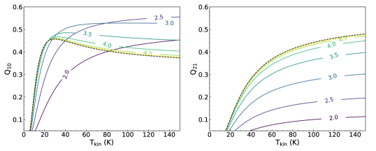
The excitation term, $Q_{\rm ul}$, which describes the fraction of C atoms in each excited state, is a function of ($n$,$T_{\rm k}$) in non-LTE conditions, and is derived analytically in the Appendix to Papadopoulos et al. (2004). A recent study of the [C i](2–1)/(1–0) line ratio found that [C i](2–1) is strongly sub-thermally excited, and [C i](1–0) presents interesting super-thermal behaviour in the range of density and temperature expected for galaxies. We illustrate the dependence of $Q_{\rm ul}$ on ($n$,$T_{\rm k}$) in Fig. 13. As discussed by Papadopoulos et al. (2022), the value of $Q_{10}$ for lower densities ($n=300$–3000 cm^-3) can exceed the LTE value at $T_{\rm k}$>20 k, but Fig. 13 shows that for a reasonable range of $n$ and $T_{\rm k}$ ($300<n<10,000$ cm^-3, $25<\mbox{$T_{\rm k}$}<80$ k) $Q_{10}$ does not go outside the range 0.35–0.53. In fact, for a uniform probability of ($2.4<\log n<4.0$) and ($25<\mbox{$T_{\rm k}$}<80$ k) the 99 per cent range for $Q_{10}$ is 0.40–0.54, median=0.48. The relative uncertainty on the calibration of C i mass from the lack of knowledge of ($n$,$T_{\rm k}$) is thus $<\pm 16$ per cent. We will therefore use the median value of $\mbox{$Q_{10}$}=0.48$ throughout, because even though we may be able to use the measured $T_{\rm d}$ to infer the galaxies with higher or lower $T_{\rm k}$ (assuming $\mbox{$T_{\rm k}$}=\alpha^{\rm TD}\,\mbox{$T_{\rm d}$}$ – see Papadopoulos et al., 2022), the lack of knowledge of the density and the super-thermal behaviour in the $J=1$ state means that there is no direct correlation between $Q_{10}$ and $T_{\rm k}$. Using sensible average parameters for MS galaxies [and SMGs], so $n$=500 [5,000] cm^-3and $T_{\rm k}$ = 40 [80] K we find only a small ($\sim$ 10  per cent) difference in the $Q_{10}$ values expected.

The LTE expressions for $Q_{10}$ and $T_{\rm x}$ should not be used (Papadopoulos et al., 2022) as $\rm Q_{10}^{LTE}$ is actually lower than the non-LTE $Q_{10}$ for densities higher than a few hundred cm^-3, and thus its use would lead to a systematic bias - e.g. for $T_{\rm k}$=60 K and n=1000cm^-3, the LTE value for $Q_{10}$ is 18  per cent lower than the appropriate non-LTE value. This would lead to an 18  per cent over-estimate of the H₂ mass using C i.

For the [C i](2–1) line, things are not so promising (Fig. 13(right)). The range of possible values of $Q_{21}$ are large, ranging from 0.07–0.37 for the 99 per cent range. The median is $Q_{21}=0.22$, giving an uncertainty range of $\pm 68$ per cent for reasonable values of ($n$,$T_{\rm k}$). Because of the sub-thermal behaviour, the [C i](2–1) line is a sensitive indicator of density (Papadopoulos et al., 2022) and galaxies with strong [C i](2–1) emission will have a larger fraction of their H₂ in a dense state.

Appendix E From pairwise variances to individual variances

We have measurements of different tracers of gas mass for several galaxies, but no direct measurements of $M_{\rm H2}$ itself. Hence, it is not possible to measure directly how well each tracer follows the gas mass. However, we do have measurements of the different tracers for each galaxy, so we can estimate the scatter in the difference between the tracers. Under some assumptions this allows us to infer the scatter between each tracer and the gas mass.

To simplify the notation, we write the log of observed quantities and corresponding standard deviation of errors as

$$x_{1} =\rm\log(L_{850}), \sigma_{1}=\rm\log(1+\sigma_{850}/L_{850}),$$ (24)

$$x_{2} =\rm\log(L^{\prime}_{\rm CO}), \sigma_{2}=\rm\log(1+\sigma_{\rm CO}/L^{\prime}_{CO}),$$

$$x_{3} =\rm\log(L^{\prime}_{\rm C\,I}), \sigma_{3}=\rm\log(1+\sigma_{\rm C\,I}/L^{\prime}_{\rm C\,I}).$$

If true value of the log of the gas mass is $\hat{m}=\log(\mbox{$M_{\rm H2}$})$, and the true values of the observed quantities are $\hat{x}_{i}$, where $i=1...3$, then we can write

$$\hat{m}=\hat{x}_{i}+\hat{a}_{i},$$ (25)

where $\hat{a}_{i}$ are the true calibration factors for each galaxy,

$$\hat{a}_{1}= -\rm\log(\hat{\alpha}_{850})$$ (26)

$$\hat{a}_{2}= \quad\rm\log(\hat{\alpha}_{CO})$$

$$\hat{a}_{3}= \quad\rm\log(\hat{\alpha}_{C\,I})$$

Note that the true values $\hat{a}_{i}$ may be different for each galaxy, depending on the individual physical conditions within the galaxies.

If we choose a particular set calibration factors for all galaxies, say $\tilde{a}_{i}$, this provides three estimates of the gas mass for each galaxy,

$$m_{i}=x_{i}+\tilde{a}_{i}$$ (27)

The error in each mass estimate is

$$m_{i}-\hat{m} =x_{i}-\hat{x_{i}}+\tilde{a}_{i}-\hat{a}_{i}$$ (28)

$$=\delta x_{i}+\delta a_{i}$$

where $\delta a_{i}$ is the difference between the true factor for this galaxy and the value we have chosen, and $\delta x_{i}$ are the measurement errors of the observations. If we assume that the errors on $x_{i}$ are not correlated with the errors on $a_{i}$, then the variance of the mass errors is given by:

$$\mathrm{var}(m_{i}-\hat{m})=\sigma_{i}^{2}+s_{i}^{2}$$ (29)

where $s_{i}^{2}$ is the variance of the true calibration factors.

The value of $s_{i}^{2}$ gives a direct measure of how accurate the particular tracer is when using a universal calibration factor for all galaxies. Without knowing the true gas mass, we do not have a direct measure of this value, but we can obtain an estimate by considering the differences between the mass measurements:

$$m_{i}-m_{j} =x_{i}-x_{j}+\tilde{a}_{i}-\tilde{a}_{j}$$ (30)

$$=\delta x_{i}-\delta x_{j}+\delta a_{i}-\delta a_{j}$$

If we ignore all co-variance terms, the variance of the differences is given by:

$$v_{ij}=\mathrm{var}(m_{i}-m_{j})=\sigma_{i}^{2}+\sigma_{j}^{2}+s_{i}^{2}+s_{j}^{2}$$ (31)

It is straightforward to re-arrange these equations to find the intrinsic variance of the calibration factors as:

$$s_{0}^{2}=\left(v_{01}-v_{12}+v_{20}\right)/2-\sigma_{0}^{2}$$ (32)

with similar equations for $s_{1}^{2}$, and $s_{2}^{2}$. So long as we have good estimates of the measurement errors, $\sigma_{i}$, for the observed quantities, we can estimate the scatter in calibration constants for each tracer. Using our dataset we have measured the variance for each pair of factors in Eqn. 31. Assuming that the co-variance between the calibration factors is zero, we use the three pair variances to estimate the intrinsic variance of the three individual calibration factors. The resulting standard deviations are $s_{\kappa}=0.1294$, $s_{\alpha}=0.1436$ and $s_{\mathrm{X}}=0.1125$, using all galaxies except the C i^cor. Values are listed in Table 3.

This analysis shows that $X_{\rm C\,I}$ has the smallest scatter between galaxies, especially when considering log $L_{\rm IR}>11$ galaxies, which is a new result, independent of any assumptions.

Appendix F A Bayesian approach to combining gas mass estimates

Our method of combining the three gas mass tracers is based on the idea that the conversion factors for any particular galaxy come from parent distributions with variances as derived in Appendix E. This means that we should allow for the expected scatter in conversion factors as well as the observational error when combining estimates from the different tracers. Using a Bayesian approach to the problem, we show the most likely mass estimate is simply the inverse variance weighted mean of the tracers, where the weights include both measurement error and the variance in conversion factors.

We continue to use the the notation as in Appendix E, where the observed quantities are $x_{i}$ and errors $\sigma_{i}$. Assuming the measurement errors are Gaussian the probability of measuring the observed value of $x_{i}$ is

$$P(x_{i}|\hat{x}_{i},\sigma_{i})={\cal N}(x_{i}|\hat{x}_{i},\sigma_{i}^{2})$$ (33)

where $\cal N$ represents the normal distribution centred on $\hat{x}_{i}$ and with variance $\sigma_{i}^{2}$. Now, for each observation we can use Bayes theorem to estimate the posterior probability that the gas mass is $m$,

$$P(m,\hat{a}_{i}|x_{i})=P(x_{i}|m,\hat{a}_{i})P(\hat{a}_{i})P(m)/P(x_{i})$$ (34)

where we have assumed $m$ and $\hat{a}_{i}$ are independent. For the prior on $\hat{a}_{i}$, we assume a normal distribution with mean $\bar{a}_{i}$ and variance $s_{i}^{2}$, as discussed in Appendix E . We assume a flat prior on $m$, implying that $P(m)$ is constant. Since $P(x_{i})$ is also constant, the position of the maximum posterior probability does not depend on the actual value of $P(m)/P(x_{i})$, and for convenience we set this to 1. Therefore:

$$\begin{split}P(m,\hat{a}_{i}|x_{i})&\propto P(x_{i}|m,\hat{a}_{i})P(\hat{a}_{i})\\ &={\cal N}(x_{i}|m-\hat{a}_{i},\sigma_{i}^{2}){\cal N}(\hat{a}_{i}|\bar{a}_{i},s_{i}^{2})\\ &={\cal N}(\hat{a}_{i}|m-x_{i},\sigma_{i}^{2}){\cal N}(\hat{a}_{i}|\bar{a}_{i},s_{i}^{2}).\end{split}$$ (35)

Here we have used Equation 25 to go from $m-\hat{a}_{i}$ to $m-x_{i}$. Since we are interested primarily in the value of the gas mass, and not explicitly in the values of the calibration factors, we can marginalise over the values of $\hat{a}_{i}$. Ignoring the uncertainties on the variances, $\sigma_{i}^{2}$ and $s_{i}^{2}$, leads to:

$$P(m|x_{i})={\cal N}(m|x_{i}+\bar{a}_{i},\sigma_{i}^{2}+s_{i}^{2}).$$ (36)

Including all three observations for the galaxy this becomes

$$\begin{split}P(m|\{x_{i}\})&=\prod_{i=1}^{3}{\cal N}(m|x_{i}+\bar{a}_{i},\sigma_{i}^{2}+s_{i}^{2})\\ &\propto\exp\left(-\sum_{i=1}^{3}\frac{(m-x_{i}-\bar{a}_{i})^{2}}{2(\sigma_{i}^{2}+s_{i}^{2})}\right).\end{split}$$ (37)

So maximising the posterior probability with respect to $m$ is equivalent to minimising $\chi^{2}$, where:

$$\chi^{2}=\sum_{i=1}^{3}\frac{(m-x_{i}-\bar{a}_{i})^{2}}{2(\sigma_{i}^{2}+s_{i}^{2})}.$$ (38)

The minimum with respect to $m$ is given by

$$\begin{split}m^{\rm opt}&=\left(\sum_{i=1}^{3}\frac{x_{i}+\bar{a_{i}}}{\sigma_{i}^{2}+s_{i}^{2}}\right)\Bigg{/}\left(\sum_{i=1}^{3}\frac{1}{\sigma_{i}^{2}+s_{i}^{2}}\right)\\ &=\left(\sum_{i=1}^{3}(x_{i}+\bar{a_{i}})w_{i}\right)\Bigg{/}\left(\sum_{i=1}^{3}w_{i}\right),\end{split}$$ (39)

where $w_{i}=1/(\sigma_{i}^{2}+s_{i}^{2})$. So the optimal mass estimate is simply the inverse variance-weighted mean of the three estimates, where each uses the mean conversion factor, and where the variance for each measure is the sum of the measurement error and the expected variance of the conversion factor.

The uncertainty on $m^{\rm opt}$ is the uncertainty on the weighted mean,

$$\sigma_{m^{\rm opt}}=1\Bigg{/}\left(\sum_{i=1}^{3}w_{i}\right).$$ (40)

The corresponding estimates of the conversion factors for a particular galaxy are then simply given by:

$$a_{i}=m-x_{i},\quad i=1...3$$ (41)

The uncertainty on the factor $a_{i}$ depends on the uncertainty on $m^{\rm opt}$, from equation 40, and the uncertainty on the measurement $x_{i}$, from equation 24. Since the estimate of $m$ depends on the measurements $x_{i}$, there is a non-zero covariance between $m$ and $x_{i}$. Allowing for this covariance, the expected uncertainty on $a_{i}$ is given by:

$$\sigma_{a_{i}}^{2}=\sigma_{\rm m^{opt}}^{2}+\sigma_{i}^{2}\left(1-\frac{2w_{i}}{\sum_{i=1}^{3}w_{i}}\right).$$ (42)

Appendix G Sensitivity of tracer to SFR and radiation field intensity

Fig. 14 shows the observable ratios, $L_{850}$/$L^{\prime}_{\rm C\,I}$ and $L_{850}$/$L^{\prime}_{\rm CO}$, as a function of $T_{\rm d}$ (left) and $L_{\rm IR}$ (right). There is no significant trend for $L_{850}$/$L^{\prime}_{\rm C\,I}$ or $L_{850}$/$L^{\prime}_{\rm CO}$ with either $T_{\rm d}$ or $L_{\rm IR}$. There is a noticeable offset to higher $L_{850}$/$L^{\prime}_{\rm C\,I}$for the C i^cor galaxies (pink diamonds), which also have lower $T_{\rm d}$ and $L_{\rm IR}$ than the other samples. As these galaxies require large corrections to $L^{\prime}_{\rm C\,I}$ in order to compare to $L_{850}$, we cannot be sure if this is a real effect, or just an under-estimate of the required correction. A larger sample of low-temperature, low-luminosity galaxies with matched apertures will be required to investigate this.

Figure 14: Luminosity ratios as a function of luminosity-weighted (peak SED) dust temperature (left) and $L_{\rm IR}$(right). In the top row, the resolved local galaxies from J19 which require aperture correction are shown as pink diamonds. In the bottom row, the galaxies with $\mbox{$f_{\rm H\,I}$}>1$ are shown as cyan diamonds, after correction following Eqn. 22. The $L^{\prime}_{\rm C\,I}$/$L^{\prime}_{\rm CO}$ ratio has a significant correlation with $T_{\rm d}$ and with $L_{\rm IR}$, and is shown in Fig. 5 in the main text.

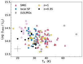
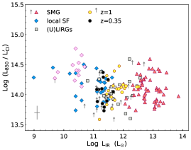
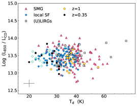
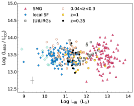
Appendix H Tests of robustness

Figure 15: Comparison of optimised conversion factors derived using three pairs of tracers, daX ($x$ axes of scatter plots) compared to using just one pair. The histograms show the offsets the parameters ($P$) $\Delta P=\log P_{\rm daX}-\log P_{S}$. The filled histogram represents galaxies free from systematic uncertainties in C i fluxes for the J19 sample (the affected C i^cor galaxies are shown as the line histogram). The median offsets are shown as the grey dotted lines on the histograms (calculated excluding the C i^cor galaxies) and are very small (0.02, 0.006, 0.04 dex for Xa, Xd, ad respectively). The offset histograms have a maximum of 0.2 dex with a r.m.s. of 0.06–0.08 dex. The scatter plots show the robust galaxies as filled circles, with C i^cor as open circles. The larger median offset for the daX–ad comparison is apparent as a non-linear trend in the $\kappa_{\rm H}$ values: for $\mbox{$\kappa_{\rm H}$}({\rm daX})<2000$ there is a persistent trend for the ad pair to return a higher $\kappa_{\rm H}$ than the daX three-pair method. The offset is also present in the $\alpha_{\rm CO}$ parameter (top-left panels) but looks more like a constant offset in the calibration rather than a non-linearity. The C i^cor galaxies (line histogram, open circles) are biased in the sense that the daX and one-pair methods produce very different values for the same parameters. The difference is smallest for the Xd sample because both daX and Xd are affected by the same corrections to the C i fluxes. The difference is more pronounced when comparing daX to ad or Xa, the reason being that the uncertain correction only affects the daX results (because the correction is between C i and dust continuum) while the ad and Xa samples do not have the C i–dust continuum pair.

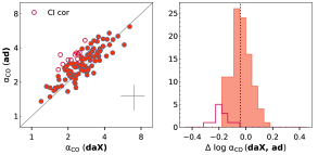
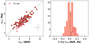
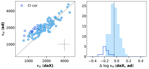
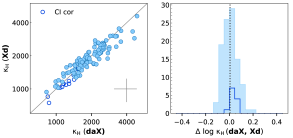
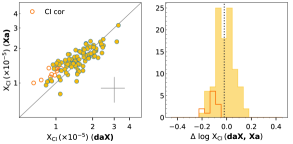
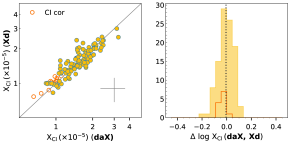
H.1 Consistency of parameter estimates

We investigated the consistency of our parameter estimates for the same galaxies when three tracers are used compared to only two. Fig. 15 shows that there is a reasonable correlation between the three-tracer and two-tracer estimates, with only small differences in the sample medians when different numbers of tracers are used. The Xd pair produces the closest match to the method with three pairs (Fig. 15 centre and lower-right panels), with no bias and a small scatter. If restricted to choosing only one pair to observe, the best choice seems to be $L_{850}$ and $L^{\prime}_{\rm C\,I}$.

H.2 Impact of using fixed vs. variable $T_{\rm mw}$

In this section we test a different approach to $T_{\rm mw}$, one of the main physical dependencies that impacts on the calibration of gas masses. To estimate gas mass from $L_{850}$, the mass-weighted dust temperature, $T_{\rm mw}$, is required. $T_{\rm mw}$ has been set to 25 k in previous studies (e.g. Scoville et al., 2014, 2016; Hughes et al., 2017), adding to the uncertainty in gas-mass estimates for individual galaxies. However, as we wish to study trends in the conversion factors, we are concerned about the possible effects of systematic trends in $T_{\rm mw}$, since these may affect the resulting behaviour of the conversion factors if ignored.

Having determined empirical relationships between $z$, $L_{\rm IR}$, SED colour ($L_{\rm IR}$/$L_{850}$) and $T_{\rm mw}$ in §2.3.1, we compare the calibration results using these empirically determined $T_{\rm mw}$ to the standard assumption of constant $T_{\rm mw}$=25 k made in the literature. Fig. 17 shows the impact of using our empirical relations (coloured points), versus keeping $T_{\rm mw}$ fixed (grey points). Each panel shows one of the affected conversion factors derived from either the ad or Xd samples. The trends with luminosity – visible for our default prescription – disappear when a constant $\mbox{$T_{\rm mw}$}=25$ k is used.

The histogram of the offsets in each conversion factor when using the empirical $T_{\rm mw}$ compared to constant $\mbox{$T_{\rm mw}$}=25$ k (Fig. 16) shows that the choice of $T_{\rm mw}$ makes no significant difference to the median values of the parameters ($<0.015$ dex). For individual galaxies, the average uncertainty introduced by using a constant $T_{\rm mw}$ is 0.046–0.06 dex (1$\sigma$), with a maximum of $\sim 0.2$ dex.

Finally, the difference in the gas-mass estimates, $M_{\rm H2}$, when using constant $T_{\rm mw}$ versus our empirical prescription is shown in Fig. 18. At lower $L_{\rm IR}$, a constant $T_{\rm mw}$ produces lower $M_{\rm H2}$ compared to our empirical method, because these galaxies are local disks which tend to have colder diffuse dust temperatures. At higher log $L_{\rm IR}$$>12$, the trend reverses as the diffuse dust temperatures increase to $\sim 30$ k.

Figure 16: Log difference between the conversion factors ($X_{\rm C\,I}$,$\delta_{\rm GDR}$,$\alpha_{\rm CO}$, $\alpha_{850}$) using the empirical relation for $T_{\rm mw}$, compared to a constant $T_{\rm mw}$ of 25 k. The median log difference for each conversion factor is shown as a vertical line, all are $<0.015$ dex, meaning the choice of $T_{\rm mw}$ for the dust does not have a significant impact on the overall average values derived from this study.

Figure 17: Running means of the conversion factors as a function of $L_{\rm IR}$. The solid coloured points use the variable $T_{\rm mw}$, as described in §2.3.1. The grey points represent the same galaxies and the same method but this time with $\mbox{$T_{\rm mw}$}=25$ k. Errors are standard errors on the mean. To better sample the full luminosity range, we have used the ad sample for this analysis, except for the $X_{\rm C\,I}$ panel which uses the Xd sample, excluding the C i^cor galaxies. The important finding is that the trends in conversion factors with $L_{\rm IR}$ disappear when a constant $T_{\rm mw}$ is assumed.

Figure 18: Difference in inferred $M_{\rm H2}$ when using the empirical prescription for $T_{\rm mw}$ (§2.3.1) compared to constant $\mbox{$T_{\rm mw}$}=25$ k. The top panel represents gas mass derived for the ad sample; the lower panel uses Xd. The pink triangles represent the C i^cor galaxies. Using a variable $T_{\rm mw}$ compared to a constant 25 k produces higher [lower] gas masses at log $L_{\rm IR}<11$ [log $L_{\rm IR}$ > 12] by up to 0.1 dex. This is not a significant issue given all other uncertainties affecting gas mass estimates.

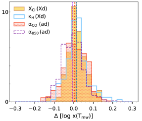
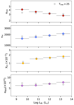
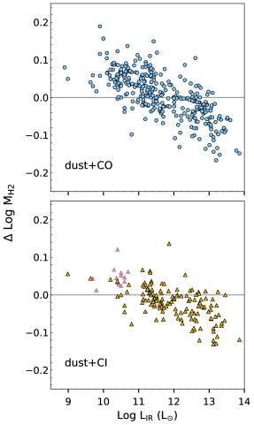
Appendix I A robust Orthogonal Distance Regression algorithm

In order to fit the most robust linear model to the data, we have employed an Orthogonal Distance Regression and included intrinsic scatter.

We use the emcee MCMC sampler (Foreman-Mackey et al., 2013) to explore the $\chi^{2}$ space and compute robust confidence intervals. Our algorithm results in parameters which are symmetric under transformation of $x$ and $y$, allowing us to utilise the full co-variance matrix, including the intrinsic scatter as a third variable.

The MCMC is set up to explore the following likelihood function:

$$LnL=-0.5\sum^{N}_{i=1}(\Delta^{2}/\sigma^{2}+\ln(\sigma^{2}/S_{2}))$$ (43)

$$\Delta={\bf v.Z}-b\,\cos(\theta)$$

with ${\bf Z}$ as the data array of $x$ and $y$ values, $b$ as the intercept and $\theta$ related to the slope as $m=tan(\theta)$. $v$ is a matrix to rotate to find the perpendicular distances, given by ${\bf v}=[-sin(\theta),cos(\theta)]$.

$$\sigma^{2}=({\bf S+\Lambda_{\rm m}.v}).{\bf v}$$

where ${\bf S}$ is the co-variance matrix. To include intrinsic scatter in the orthogonal direction, as well as measurement errors into the fitting, we add a term to the co-variance matrix, as suggested in Foreman-Mackey (2017):

$${\bf\Lambda_{\rm m}}=\begin{pmatrix}\tan(\theta)^{2}&-\tan(\theta)\\ -\tan(\theta)&1.0\\ \end{pmatrix}\times\cos(\theta)^{2}\times e^{2\,\ln(\lambda)}$$ (44)

$$S_{2}=({\bf S.v}).{\bf v}$$

The initial conditions were given by the ordinary least-squares fit parameters for variance in the $y$ direction. The run was checked to ensure adequate burn-in and independence between samples. We used 32 random walkers with 6,000 steps each.

References

- Aalto et al. (1995) Aalto S., Booth R. S., Black J. H., Johansson L. E. B., 1995, A&A, 300, 369
- Accurso et al. (2017) Accurso G., et al., 2017, MNRAS, 470, 4750
- Alaghband-Zadeh et al. (2013) Alaghband-Zadeh S., et al., 2013, MNRAS, 435, 1493
- Alatalo et al. (2013) Alatalo K., et al., 2013, MNRAS, 432, 1796
- Alatalo et al. (2016) Alatalo K., et al., 2016, ApJ, 827, 106
- Albrecht et al. (2007) Albrecht M., Krügel E., Chini R., 2007, A&A, 462, 575
- Amorín et al. (2016) Amorín R., Muñoz-Tuñón C., Aguerri J. A. L., Planesas P., 2016, A&A, 588, A23
- Ao et al. (2008) Ao Y., Weiß A., Downes D., Walter F., Henkel C., Menten K. M., 2008, A&A, 491, 747
- Aravena et al. (2016) Aravena M., et al., 2016, MNRAS, 457, 4406
- Armus et al. (2009) Armus L., et al., 2009, PASP, 121, 559
- Baan et al. (2008) Baan W. A., Henkel C., Loenen A. F., Baudry A., Wiklind T., 2008, A&A, 477, 747
- Baker et al. (2022) Baker W. M., Maiolino R., Bluck A. F. L., Lin L., Ellison S. L., Belfiore F., Pan H.-A., Thorp M., 2022, MNRAS, 510, 3622
- Bakx et al. (2020) Bakx T. J. L. C., et al., 2020, MNRAS, 496, 2372
- Behroozi et al. (2013) Behroozi P. S., Wechsler R. H., Conroy C., 2013, ApJ, 770, 57
- Bendo et al. (2015) Bendo G. J., et al., 2015, MNRAS, 448, 135
- Berta et al. (2021) Berta S., et al., 2021, A&A, 646, A122
- Béthermin et al. (2018) Béthermin M., et al., 2018, A&A, 620, A115
- Beuther et al. (2014) Beuther H., et al., 2014, A&A, 571, A53
- Bianchi et al. (2019) Bianchi S., et al., 2019, A&A, 631, A102
- Bigiel et al. (2008) Bigiel F., Leroy A., Walter F., Brinks E., de Blok W. J. G., Madore B., Thornley M. D., 2008, AJ, 136, 2846
- Bisbas et al. (2015) Bisbas T. G., Papadopoulos P. P., Viti S., 2015, ApJ, 803, 37
- Bisbas et al. (2017) Bisbas T. G., van Dishoeck E. F., Papadopoulos P. P., Szűcs L., Bialy S., Zhang Z.-Y., 2017, ApJ, 839, 90
- Bisbas et al. (2021) Bisbas T. G., Tan J. C., Tanaka K. E. I., 2021, MNRAS, 502, 2701
- Blain & Longair (1993) Blain A. W., Longair M. S., 1993, MNRAS, 264, 509
- Blitz & Rosolowsky (2006) Blitz L., Rosolowsky E., 2006, ApJ, 650, 933
- Bolatto et al. (2013) Bolatto A. D., Wolfire M., Leroy A. K., 2013, ARA&A, 51, 207
- Bolatto et al. (2017) Bolatto A. D., et al., 2017, ApJ, 846, 159
- Boogaard et al. (2020) Boogaard L. A., et al., 2020, ApJ, 902, 109
- Bothwell et al. (2013) Bothwell M. S., et al., 2013, MNRAS, 429, 3047
- Bothwell et al. (2014) Bothwell M. S., et al., 2014, MNRAS, 445, 2599
- Bothwell et al. (2017) Bothwell M. S., et al., 2017, MNRAS, 466, 2825
- Boulanger et al. (1996) Boulanger F., Abergel A., Bernard J.-P., Burton W. B., Desert F.-X., Hartmann D., Lagache G., Puget J.-L., 1996, A&A, 312, 256
- Bourne et al. (2019) Bourne N., Dunlop J. S., Simpson J. M., Rowlands K. E., Geach J. E., McLeod D. J., 2019, MNRAS, 482, 3135
- Bryant & Scoville (1996) Bryant P. M., Scoville N. Z., 1996, ApJ, 457, 678
- Bussmann et al. (2013) Bussmann R. S., et al., 2013, ApJ, 779, 25
- Bussmann et al. (2015) Bussmann R. S., et al., 2015, ApJ, 812, 43
- Cañameras et al. (2015) Cañameras R., et al., 2015, A&A, 581, A105
- Cao et al. (2017) Cao Y., Wong T., Xue R., Bolatto A. D., Blitz L., Vogel S. N., Leroy A. K., Rosolowsky E., 2017, ApJ, 847, 33
- Carilli et al. (2010) Carilli C. L., et al., 2010, ApJ, 714, 1407
- Carilli et al. (2011) Carilli C. L., Hodge J., Walter F., Riechers D., Daddi E., Dannerbauer H., Morrison G. E., 2011, ApJ, 739, L33
- Casasola et al. (2020) Casasola V., et al., 2020, A&A, 633, A100
- Casoli et al. (1996) Casoli F., Dickey J., Kazes I., Boselli A., Gavazzi G., Jore K., 1996, A&AS, 116, 193
- Chapman et al. (2005) Chapman S. C., Blain A. W., Smail I., Ivison R. J., 2005, ApJ, 622, 772
- Chapman et al. (2010) Chapman S. C., et al., 2010, MNRAS, 409, L13
- Chen et al. (2015) Chen B. Q., Liu X. W., Yuan H. B., Huang Y., Xiang M. S., 2015, MNRAS, 448, 2187
- Chen et al. (2018) Chen L.-H., Hirashita H., Hou K.-C., Aoyama S., Shimizu I., Nagamine K., 2018, MNRAS, 474, 1545
- Chu et al. (2017) Chu J. K., et al., 2017, ApJS, 229, 25
- Chung et al. (2009) Chung A., Narayanan G., Yun M. S., Heyer M., Erickson N. R., 2009, AJ, 138, 858
- Cicone et al. (2018) Cicone C., et al., 2018, ApJ, 863, 143
- Ciesla et al. (2020) Ciesla L., et al., 2020, A&A, 635, A27
- Clark et al. (2015) Clark C. J. R., et al., 2015, MNRAS, 452, 397
- Clark et al. (2016) Clark C. J. R., Schofield S. P., Gomez H. L., Davies J. I., 2016, MNRAS, 459, 1646
- Clark et al. (2018) Clark C. J. R., et al., 2018, A&A, 609, A37
- Clark et al. (2019a) Clark P. C., Glover S. C. O., Ragan S. E., Duarte-Cabral A., 2019a, MNRAS, 486, 4622
- Clark et al. (2019b) Clark C. J. R., et al., 2019b, MNRAS, 489, 5256
- Cooray et al. (2014) Cooray A., et al., 2014, ApJ, 790, 40
- Coppin et al. (2006) Coppin K., et al., 2006, MNRAS, 372, 1621
- Cormier et al. (2018) Cormier D., et al., 2018, MNRAS, 475, 3909
- Cox et al. (2011) Cox P., et al., 2011, ApJ, 740, 63
- Crocker et al. (2019) Crocker A. F., et al., 2019, ApJ, 887, 105
- Curran et al. (2000) Curran S. J., Aalto S., Booth R. S., 2000, A&AS, 141, 193
- Daddi et al. (2009) Daddi E., Dannerbauer H., Krips M., Walter F., Dickinson M., Elbaz D., Morrison G. E., 2009, ApJ, 695, L176
- Dale & Helou (2002) Dale D. A., Helou G., 2002, ApJ, 576, 159
- Dale et al. (2012) Dale D. A., et al., 2012, ApJ, 745, 95
- Dale et al. (2017) Dale D. A., et al., 2017, ApJ, 837, 90
- Danielson et al. (2011) Danielson A. L. R., et al., 2011, MNRAS, 410, 1687
- Dannerbauer et al. (2019) Dannerbauer H., Harrington K., Díaz-Sánchez A., Iglesias-Groth S., Rebolo R., Genova-Santos R. T., Krips M., 2019, AJ, 158, 34
- De Vis et al. (2021) De Vis P., Maddox S. J., Gomez H. L., Jones A. P., Dunne L., 2021, MNRAS, 505, 3228
- Decarli et al. (2016) Decarli R., et al., 2016, ApJ, 833, 69
- Decarli et al. (2019) Decarli R., et al., 2019, ApJ, 882, 138
- Díaz-Santos et al. (2017) Díaz-Santos T., et al., 2017, ApJ, 846, 32
- Dickman et al. (1986) Dickman R. L., Snell R. L., Schloerb F. P., 1986, ApJ, 309, 326
- Downes & Solomon (1998) Downes D., Solomon P. M., 1998, ApJ, 507, 615
- Draine (2003) Draine B. T., 2003, ARA&A, 41, 241
- Draine (2009) Draine B. T., 2009, in Henning T., Grün E., Steinacker J., eds, Astronomical Society of the Pacific Conference Series Vol. 414, Cosmic Dust - Near and Far. p. 453 (arXiv:0903.1658)
- Draine & Hensley (2021) Draine B. T., Hensley B. S., 2021, ApJ, 909, 94
- Draine & Li (2007) Draine B. T., Li A., 2007, ApJ, 657, 810
- Draine et al. (2007) Draine B. T., et al., 2007, ApJ, 663, 866
- Draine et al. (2014) Draine B. T., et al., 2014, ApJ, 780, 172
- Drew et al. (2020) Drew P. M., Casey C. M., Cooray A., Whitaker K. E., 2020, ApJ, 892, 104
- Driver et al. (2018) Driver S. P., et al., 2018, MNRAS, 475, 2891
- Dunne & Eales (2001) Dunne L., Eales S. A., 2001, MNRAS, 327, 697
- Dunne et al. (2000) Dunne L., Eales S., Edmunds M., Ivison R., Alexander P., Clements D. L., 2000, MNRAS, 315, 115
- Dunne et al. (2003) Dunne L., Eales S., Ivison R., Morgan H., Edmunds M., 2003, Nature, 424, 285
- Dunne et al. (2011) Dunne L., et al., 2011, MNRAS, 417, 1510
- Dunne et al. (2021) Dunne L., Maddox S. J., Vlahakis C., Gomez H. L., 2021, MNRAS, 501, 2573
- Dye et al. (2015) Dye S., et al., 2015, MNRAS, 452, 2258
- Eales et al. (2010) Eales S., et al., 2010, PASP, 122, 499
- Eales et al. (2012) Eales S., et al., 2012, ApJ, 761, 168
- Elmegreen (1993) Elmegreen B. G., 1993, ApJ, 411, 170
- Emonts et al. (2013) Emonts B. H. C., et al., 2013, MNRAS, 430, 3465
- Emonts et al. (2018) Emonts B. H. C., et al., 2018, MNRAS, 477, L60
- Engel et al. (2010) Engel H., et al., 2010, ApJ, 724, 233
- Enia et al. (2018) Enia A., et al., 2018, MNRAS, 475, 3467
- Falgarone et al. (1998) Falgarone E., Panis J. F., Heithausen A., Perault M., Stutzki J., Puget J. L., Bensch F., 1998, A&A, 331, 669
- Falgarone et al. (2017) Falgarone E., et al., 2017, Nature, 548, 430
- Falstad et al. (2021) Falstad N., et al., 2021, A&A, 649, A105
- Flagey et al. (2009) Flagey N., et al., 2009, ApJ, 701, 1450
- Foreman-Mackey (2016) Foreman-Mackey D., 2016, Journal of Open Source Software, 1, 24
- Foreman-Mackey (2017) Foreman-Mackey D., 2017, Fitting a plane to data, doi:10.5281/zenodo.3221478. , https://doi.org/10.5281/zenodo.3221478
- Foreman-Mackey et al. (2013) Foreman-Mackey D., Hogg D. W., Lang D., Goodman J., 2013, PASP, 125, 306
- Foyle et al. (2012) Foyle K., et al., 2012, MNRAS, 421, 2917
- Frayer et al. (2011) Frayer D. T., et al., 2011, ApJ, 726, L22
- Frayer et al. (2018) Frayer D. T., Maddalena R. J., Ivison R. J., Smail I., Blain A. W., Vanden Bout P., 2018, ApJ, 860, 87
- Frerking et al. (1989) Frerking M. A., Keene J., Blake G. A., Phillips T. G., 1989, ApJ, 344, 311
- Galametz et al. (2011) Galametz M., Madden S. C., Galliano F., Hony S., Bendo G. J., Sauvage M., 2011, A&A, 532, A56
- Gao & Solomon (2004) Gao Y., Solomon P. M., 2004, ApJ, 606, 271
- García-Burillo et al. (2012) García-Burillo S., Usero A., Alonso-Herrero A., Graciá-Carpio J., Pereira-Santaella M., Colina L., Planesas P., Arribas S., 2012, A&A, 539, A8
- Genzel et al. (2010) Genzel R., et al., 2010, MNRAS, 407, 2091
- Genzel et al. (2015) Genzel R., et al., 2015, ApJ, 800, 20
- Glover & Clark (2016) Glover S. C. O., Clark P. C., 2016, MNRAS, 456, 3596
- Gómez-Guijarro et al. (2019) Gómez-Guijarro C., et al., 2019, ApJ, 872, 117
- Gong et al. (2020) Gong M., Ostriker E. C., Kim C.-G., Kim J.-G., 2020, ApJ, 903, 142
- Greve et al. (2005) Greve T. R., et al., 2005, MNRAS, 359, 1165
- Greve et al. (2014) Greve T. R., et al., 2014, ApJ, 794, 142
- Groves et al. (2015) Groves B. A., et al., 2015, ApJ, 799, 96
- Hainline et al. (2006) Hainline L. J., Blain A. W., Greve T. R., Chapman S. C., Smail I., Ivison R. J., 2006, ApJ, 650, 614
- Harrington et al. (2021) Harrington K. C., et al., 2021, ApJ, 908, 95
- Harris et al. (2010) Harris A. I., Baker A. J., Zonak S. G., Sharon C. E., Genzel R., Rauch K., Watts G., Creager R., 2010, ApJ, 723, 1139
- Heintz & Watson (2020) Heintz K. E., Watson D., 2020, ApJ, 889, L7
- Hensley & Draine (2021) Hensley B. S., Draine B. T., 2021, ApJ, 906, 73
- Herrero-Illana et al. (2019) Herrero-Illana R., et al., 2019, A&A, 628, A71
- Hodge et al. (2013) Hodge J. A., et al., 2013, ApJ, 768, 91
- Hogg et al. (2010) Hogg D. W., Bovy J., Lang D., 2010, arXiv e-prints, p. arXiv:1008.4686
- Honma et al. (1995) Honma M., Sofue Y., Arimoto N., 1995, A&A, 304, 1
- Hughes et al. (2017) Hughes T. M., et al., 2017, MNRAS, 468, L103
- Hunt et al. (2015) Hunt L. K., et al., 2015, A&A, 583, A114
- Hunt et al. (2019) Hunt L. K., et al., 2019, A&A, 621, A51
- Huynh et al. (2017) Huynh M. T., et al., 2017, MNRAS, 467, 1222
- Ikeda et al. (2002) Ikeda M., Oka T., Tatematsu K., Sekimoto Y., Yamamoto S., 2002, ApJS, 139, 467
- Iono et al. (2012) Iono D., et al., 2012, PASJ, 64, L2
- Israel (1997) Israel F. P., 1997, A&A, 328, 471
- Israel (2020) Israel F. P., 2020, A&A, 635, A131
- Ivison et al. (2010) Ivison R. J., et al., 2010, A&A, 518, L35
- Ivison et al. (2011) Ivison R. J., Papadopoulos P. P., Smail I., Greve T. R., Thomson A. P., Xilouris E. M., Chapman S. C., 2011, MNRAS, 412, 1913
- Ivison et al. (2013) Ivison R. J., et al., 2013, ApJ, 772, 137
- Izumi et al. (2020) Izumi T., et al., 2020, ApJ, 898, 75
- James et al. (2002) James A., Dunne L., Eales S., Edmunds M. G., 2002, MNRAS, 335, 753
- Jiao et al. (2017) Jiao Q., Zhao Y., Zhu M., Lu N., Gao Y., Zhang Z.-Y., 2017, ApJ, 840, L18
- Jiao et al. (2019) Jiao Q., et al., 2019, ApJ, 880, 133
- Jiao et al. (2021) Jiao Q., Gao Y., Zhao Y., 2021, MNRAS, 504, 2360
- Jin et al. (2019) Jin S., et al., 2019, ApJ, 887, 144
- Jones (2018) Jones A. P., 2018, arXiv e-prints, p. arXiv:1804.10628
- Jones et al. (2017) Jones A. P., Köhler M., Ysard N., Bocchio M., Verstraete L., 2017, A&A, 602, A46
- Kaasinen et al. (2019) Kaasinen M., et al., 2019, ApJ, 880, 15
- Kamenetzky et al. (2014) Kamenetzky J., Rangwala N., Glenn J., Maloney P. R., Conley A., 2014, ApJ, 795, 174
- Kamenetzky et al. (2016) Kamenetzky J., Rangwala N., Glenn J., Maloney P. R., Conley A., 2016, ApJ, 829, 93
- Kennicutt (1998) Kennicutt Jr. R. C., 1998, ApJ, 498, 541
- Kennicutt et al. (2011) Kennicutt R. C., et al., 2011, PASP, 123, 1347
- Keres et al. (2003) Keres D., Yun M. S., Young J. S., 2003, ApJ, 582, 659
- Koda et al. (2011) Koda J., et al., 2011, ApJS, 193, 19
- Köhler et al. (2015) Köhler M., Ysard N., Jones A. P., 2015, A&A, 579, A15
- Koribalski et al. (2018) Koribalski B. S., et al., 2018, MNRAS, 478, 1611
- Kovács et al. (2006) Kovács A., Chapman S. C., Dowell C. D., Blain A. W., Ivison R. J., Smail I., Phillips T. G., 2006, ApJ, 650, 592
- Kuno et al. (2007) Kuno N., et al., 2007, PASJ, 59, 117
- Lagos et al. (2015) Lagos C. d. P., et al., 2015, MNRAS, 452, 3815
- Lapham & Young (2019) Lapham R. C., Young L. M., 2019, ApJ, 875, 3
- Leroy et al. (2008) Leroy A. K., Walter F., Brinks E., Bigiel F., de Blok W. J. G., Madore B., Thornley M. D., 2008, AJ, 136, 2782
- Leroy et al. (2011) Leroy A. K., et al., 2011, ApJ, 737, 12
- Lestrade et al. (2011) Lestrade J.-F., Carilli C. L., Thanjavur K., Kneib J.-P., Riechers D. A., Bertoldi F., Walter F., Omont A., 2011, ApJ, 739, L30
- Leung et al. (2019) Leung T. K. D., et al., 2019, ApJ, 871, 85
- Li & Draine (2001) Li A., Draine B. T., 2001, ApJ, 554, 778
- Lilly et al. (1996) Lilly S. J., Le Fevre O., Hammer F., Crampton D., 1996, ApJ, 460, L1
- Liszt (2011) Liszt H. S., 2011, A&A, 527, A45
- Liu et al. (2015) Liu D., Gao Y., Isaak K., Daddi E., Yang C., Lu N., van der Werf P., 2015, ApJ, 810, L14
- Liu et al. (2021) Liu D., et al., 2021, ApJ, 909, 56
- Lu et al. (2017) Lu N., et al., 2017, ApJS, 230, 1
- Madau & Dickinson (2014) Madau P., Dickinson M., 2014, ARA&A, 52, 415
- Madau et al. (1996) Madau P., Ferguson H. C., Dickinson M. E., Giavalisco M., Steidel C. C., Fruchter A., 1996, MNRAS, 283, 1388
- Madden et al. (1997) Madden S. C., Poglitsch A., Geis N., Stacey G. J., Townes C. H., 1997, ApJ, 483, 200
- Magdis et al. (2012) Magdis G. E., et al., 2012, ApJ, 760, 6
- Magnelli et al. (2012) Magnelli B., et al., 2012, A&A, 539, A155
- McKean et al. (2011) McKean J. P., Berciano Alba A., Volino F., Tudose V., Garrett M. A., Loenen A. F., Paragi Z., Wucknitz O., 2011, MNRAS, 414, L11
- Messias et al. (2014) Messias H., et al., 2014, A&A, 568, A92
- Messias et al. (2019) Messias H., et al., 2019, MNRAS, 486, 2366
- Michiyama et al. (2020) Michiyama T., et al., 2020, ApJ, 897, L19
- Mirabel et al. (1990) Mirabel I. F., Booth R. S., Garay G., Johansson L. E. B., Sanders D. B., 1990, A&A, 236, 327
- Muñoz-Mateos et al. (2009) Muñoz-Mateos J. C., et al., 2009, ApJ, 701, 1965
- Narayanan et al. (2011) Narayanan D., Krumholz M., Ostriker E. C., Hernquist L., 2011, MNRAS, 418, 664
- Negrello et al. (2014) Negrello M., et al., 2014, MNRAS, 440, 1999
- Negrello et al. (2017) Negrello M., et al., 2017, MNRAS, 465, 3558
- Neri et al. (2020) Neri R., et al., 2020, A&A, 635, A7
- Nesvadba et al. (2019) Nesvadba N. P. H., Cañameras R., Kneissl R., Koenig S., Yang C., Le Floc’h E., Omont A., Scott D., 2019, A&A, 624, A23
- Obreschkow et al. (2009) Obreschkow D., Croton D., De Lucia G., Khochfar S., Rawlings S., 2009, ApJ, 698, 1467
- Offner et al. (2014) Offner S. S. R., Bisbas T. G., Bell T. A., Viti S., 2014, MNRAS, 440, L81
- Oliver et al. (2012) Oliver S. J., et al., 2012, MNRAS, 424, 1614
- Orellana et al. (2017) Orellana G., et al., 2017, A&A, 602, A68
- Oteo et al. (2017) Oteo I., et al., 2017, ApJ, 850, 170
- Oteo et al. (2018) Oteo I., et al., 2018, ApJ, 856, 72
- Pak et al. (1998) Pak S., Jaffe D. T., van Dishoeck E. F., Johansson L. E. B., Booth R. S., 1998, ApJ, 498, 735
- Papadopoulos (2010) Papadopoulos P. P., 2010, ApJ, 720, 226
- Papadopoulos & Geach (2012) Papadopoulos P. P., Geach J. E., 2012, ApJ, 757, 157
- Papadopoulos & Greve (2004) Papadopoulos P. P., Greve T. R., 2004, ApJ, 615, L29
- Papadopoulos et al. (2002) Papadopoulos P. P., Thi W.-F., Viti S., 2002, ApJ, 579, 270
- Papadopoulos et al. (2004) Papadopoulos P. P., Thi W.-F., Viti S., 2004, MNRAS, 351, 147
- Papadopoulos et al. (2012a) Papadopoulos P. P., van der Werf P. P., Xilouris E. M., Isaak K. G., Gao Y., Mühle S., 2012a, MNRAS, 426, 2601
- Papadopoulos et al. (2012b) Papadopoulos P. P., van der Werf P., Xilouris E., Isaak K. G., Gao Y., 2012b, ApJ, 751, 10
- Papadopoulos et al. (2014) Papadopoulos P. P., et al., 2014, ApJ, 788, 153
- Papadopoulos et al. (2018) Papadopoulos P. P., Bisbas T. G., Zhang Z.-Y., 2018, MNRAS, 478, 1716
- Papadopoulos et al. (2022) Papadopoulos P., Dunne L., Maddox S., 2022, MNRAS, 510, 725
- Pappalardo et al. (2012) Pappalardo C., et al., 2012, A&A, 545, A75
- Pavesi et al. (2018a) Pavesi R., et al., 2018a, ApJ, 861, 43
- Pavesi et al. (2018b) Pavesi R., et al., 2018b, ApJ, 864, 49
- Pelupessy & Papadopoulos (2009) Pelupessy F. I., Papadopoulos P. P., 2009, ApJ, 707, 954
- Pereira-Santaella et al. (2013) Pereira-Santaella M., et al., 2013, ApJ, 768, 55
- Pérez-Beaupuits et al. (2015) Pérez-Beaupuits J. P., Stutzki J., Ossenkopf V., Spaans M., Güsten R., Wiesemeyer H., 2015, A&A, 575, A9
- Perna et al. (2018) Perna M., et al., 2018, A&A, 619, A90
- Péroux & Howk (2020) Péroux C., Howk J. C., 2020, ARA&A, 58, 363
- Planck Collaboration XI (2014) Planck Collaboration XI 2014, A&A, 571, A11
- Planck Collaboration XIX (2011) Planck Collaboration XIX 2011, A&A, 536, A19
- Planck Collaboration XVII (2014) Planck Collaboration XVII 2014, A&A, 566, A55
- Planck Collaboration XXIX (2016) Planck Collaboration XXIX 2016, A&A, 586, A132
- Planck Collaboration et al. (2011) Planck Collaboration et al., 2011, A&A, 536, A1
- Plume et al. (1999) Plume R., Jaffe D. T., Tatematsu K., Evans Neal J. I., Keene J., 1999, ApJ, 512, 768
- Popping et al. (2014) Popping G., Somerville R. S., Trager S. C., 2014, MNRAS, 442, 2398
- Popping et al. (2017) Popping G., et al., 2017, A&A, 602, A11
- Priestley & Whitworth (2020) Priestley F. D., Whitworth A. P., 2020, MNRAS, 494, L48
- Remy et al. (2017) Remy Q., Grenier I. A., Marshall D. J., Casand jian J. M., 2017, A&A, 601, A78
- Remy et al. (2018) Remy Q., Grenier I. A., Marshall D. J., Casand jian J. M., 2018, A&A, 616, A71
- Rhee et al. (2018) Rhee J., Lah P., Briggs F. H., Chengalur J. N., Colless M., Willner S. P., Ashby M. L. N., Le Fèvre O., 2018, MNRAS, 473, 1879
- Riechers et al. (2011) Riechers D. A., Hodge J., Walter F., Carilli C. L., Bertoldi F., 2011, ApJ, 739, L31
- Riechers et al. (2013) Riechers D. A., et al., 2013, Nature, 496, 329
- Riechers et al. (2019) Riechers D. A., et al., 2019, ApJ, 872, 7
- Riechers et al. (2020) Riechers D. A., et al., 2020, ApJ, 896, L21
- Rosenberg et al. (2015) Rosenberg M. J. F., et al., 2015, ApJ, 801, 72
- Rowlands et al. (2014) Rowlands K., et al., 2014, MNRAS, 441, 1017
- Saintonge et al. (2016) Saintonge A., et al., 2016, MNRAS, 462, 1749
- Saintonge et al. (2017) Saintonge A., et al., 2017, ApJS, 233, 22
- Saito et al. (2020) Saito T., et al., 2020, MNRAS, 497, 3591
- Salak et al. (2019) Salak D., Nakai N., Seta M., Miyamoto Y., 2019, ApJ, 887, 143
- Sandstrom et al. (2013) Sandstrom K. M., et al., 2013, ApJ, 777, 5
- Santini et al. (2010) Santini P., et al., 2010, A&A, 518, L154
- Schilke et al. (1993) Schilke P., Carlstrom J. E., Keene J., Phillips T. G., 1993, ApJ, 417, L67
- Schneider et al. (2003) Schneider N., Simon R., Kramer C., Kraemer K., Stutzki J., Mookerjea B., 2003, A&A, 406, 915
- Schruba et al. (2011) Schruba A., et al., 2011, AJ, 142, 37
- Schruba et al. (2012) Schruba A., et al., 2012, AJ, 143, 138
- Scoville et al. (2014) Scoville N., et al., 2014, ApJ, 783, 84
- Scoville et al. (2016) Scoville N., et al., 2016, ApJ, 820, 83
- Scoville et al. (2017) Scoville N., et al., 2017, ApJ, 837, 150
- Seaquist et al. (2004) Seaquist E., Yao L., Dunne L., Cameron H., 2004, MNRAS, 349, 1428
- Sharon et al. (2013) Sharon C. E., Baker A. J., Harris A. I., Thomson A. P., 2013, ApJ, 765, 6
- Sharon et al. (2016) Sharon C. E., Riechers D. A., Hodge J., Carilli C. L., Walter F., Weiß A., Knudsen K. K., Wagg J., 2016, ApJ, 827, 18
- Sodroski et al. (1997) Sodroski T. J., Odegard N., Arendt R. G., Dwek E., Weiland J. L., Hauser M. G., Kelsall T., 1997, ApJ, 480, 173
- Solomon & Vanden Bout (2005) Solomon P. M., Vanden Bout P. A., 2005, ARA&A, 43, 677
- Sorai et al. (2019) Sorai K., et al., 2019, PASJ, 71, S14
- Spekkens et al. (2004) Spekkens K., Irwin J. A., Saikia D. J., 2004, MNRAS, 352, 1145
- Spilker et al. (2016) Spilker J. S., et al., 2016, ApJ, 826, 112
- Stevens et al. (2005) Stevens J. A., Amure M., Gear W. K., 2005, MNRAS, 357, 361
- Stutzki et al. (1997) Stutzki J., et al., 1997, ApJ, 477, L33
- Swinbank et al. (2014) Swinbank A. M., et al., 2014, MNRAS, 438, 1267
- Tacconi et al. (2006) Tacconi L. J., et al., 2006, ApJ, 640, 228
- Tacconi et al. (2008) Tacconi L. J., et al., 2008, ApJ, 680, 246
- Tan et al. (2014) Tan Q., et al., 2014, A&A, 569, A98
- Tauber et al. (1991) Tauber J. A., Goldsmith P. F., Dickman R. L., 1991, ApJ, 375, 635
- Tauber et al. (1995) Tauber J. A., Lis D. C., Keene J., Schilke P., Buettgenbach T. H., 1995, A&A, 297, 567
- Thomas et al. (2002) Thomas H. C., Dunne L., Clemens M. S., Alexand er P., Eales S., Green D. A., 2002, MNRAS, 329, 747
- Thomas et al. (2004) Thomas H. C., Dunne L., Green D. A., Clemens M. S., Alexander P., Eales S., 2004, MNRAS, 348, 1197
- Thomson et al. (2012) Thomson A. P., et al., 2012, MNRAS, 425, 2203
- Thuan et al. (2016) Thuan T. X., Goehring K. M., Hibbard J. E., Izotov Y. I., Hunt L. K., 2016, MNRAS, 463, 4268
- Tielens & Hollenbach (1985) Tielens A. G. G. M., Hollenbach D., 1985, ApJ, 291, 722
- Tinney et al. (1990) Tinney C. G., Scoville N. Z., Sanders D. B., Soifer B. T., 1990, ApJ, 362, 473
- Ueda et al. (2014) Ueda J., et al., 2014, ApJS, 214, 1
- Valentino et al. (2018) Valentino F., et al., 2018, ApJ, 869, 27
- Valentino et al. (2020) Valentino F., et al., 2020, ApJ, 890, 24
- Vieira et al. (2010) Vieira J. D., et al., 2010, ApJ, 719, 763
- Villanueva et al. (2017) Villanueva V., et al., 2017, MNRAS, 470, 3775
- Walter et al. (2011) Walter F., Weiß A., Downes D., Decarli R., Henkel C., 2011, ApJ, 730, 18
- Walter et al. (2012) Walter F., et al., 2012, Nature, 486, 233
- Walter et al. (2014) Walter F., et al., 2014, ApJ, 782, 79
- Wang et al. (2018) Wang T., et al., 2018, ApJ, 867, L29
- Weiß et al. (2003) Weiß A., Henkel C., Downes D., Walter F., 2003, A&A, 409, L41
- Weiß et al. (2005) Weiß A., Downes D., Henkel C., Walter F., 2005, A&A, 429, L25
- Weiß et al. (2007) Weiß A., Downes D., Neri R., Walter F., Henkel C., Wilner D. J., Wagg J., Wiklind T., 2007, A&A, 467, 955
- Weiß et al. (2013) Weiß A., et al., 2013, ApJ, 767, 88
- White et al. (1994) White G. J., Ellison B., Claude S., Dent W. R. F., Matheson D. N., 1994, A&A, 284, L23
- Wilson et al. (2008) Wilson C. D., et al., 2008, ApJS, 178, 189
- Wong & Blitz (2002) Wong T., Blitz L., 2002, ApJ, 569, 157
- Wong et al. (2013) Wong T., et al., 2013, ApJ, 777, L4
- Wong et al. (2017) Wong K. C., Ishida T., Tamura Y., Suyu S. H., Oguri M., Matsushita S., 2017, ApJ, 843, L35
- Wu et al. (2009) Wu J., Vanden Bout P. A., Evans Neal J. I., Dunham M. M., 2009, ApJ, 707, 988
- Yamashita et al. (2017) Yamashita T., et al., 2017, ApJ, 844, 96
- Yang et al. (2017) Yang C., et al., 2017, A&A, 608, A144
- Yang et al. (2019) Yang C., et al., 2019, A&A, 624, A138
- Yao et al. (2003) Yao L., Seaquist E. R., Kuno N., Dunne L., 2003, ApJ, 588, 771
- Young et al. (1995) Young J. S., et al., 1995, ApJS, 98, 219
- Young et al. (2008) Young L. M., Bureau M., Cappellari M., 2008, ApJ, 676, 317
- Ysard et al. (2013) Ysard N., et al., 2013, A&A, 559, A133
- Ysard et al. (2015) Ysard N., Köhler M., Jones A., Miville-Deschênes M.-A., Abergel A., Fanciullo L., 2015, A&A, 577, A110
- Ysard et al. (2018) Ysard N., Jones A. P., Demyk K., Boutéraon T., Koehler M., 2018, A&A, 617, A124
- Zafar et al. (2013) Zafar T., Péroux C., Popping A., Milliard B., Deharveng J. M., Frank S., 2013, A&A, 556, A141
- Zhang et al. (2016) Zhang Z.-Y., Papadopoulos P. P., Ivison R. J., Galametz M., Smith M. W. L., Xilouris E. M., 2016, Royal Society Open Science, 3, 160025
- Zhu et al. (1999) Zhu M., Seaquist E. R., Davoust E., Frayer D. T., Bushouse H. A., 1999, AJ, 118, 145
- Zmuidzinas et al. (1988) Zmuidzinas J., Betz A. L., Boreiko R. T., Goldhaber D. M., 1988, ApJ, 335, 774
- Zwaan et al. (2004) Zwaan M. A., et al., 2004, MNRAS, 350, 1210
- da Cunha et al. (2008) da Cunha E., Charlot S., Elbaz D., 2008, MNRAS, 388, 1595
- da Cunha et al. (2013) da Cunha E., et al., 2013, ApJ, 766, 13
- da Cunha et al. (2015) da Cunha E., et al., 2015, ApJ, 806, 110