On the Age of Status Updates in Unreliable Multi-Source M/G/1 Queueing Systems

Muthukrishnan Senthil Kumar, , Aresh Dadlani, , Masoumeh Moradian, Ahmad Khonsari, Theodoros A. Tsiftsis This work was supported by the National Natural Science Foundation of China under Grant 62071202.Muthukrishnan Senthil Kumar is with the Department of Applied Mathematics and Computational Sciences, PSG College of Technology, Coimbatore 641004, India (e-mail: msk.amcs@psgtech.ac.in).Aresh Dadlani is with the Faculty of Arts - Interdisciplinary Studies, University of Alberta, Edmonton, AB T6G 2E7, Canada, and also with the Department of Electrical and Computer Engineering, Nazarbayev University, Astana 010000, Kazakhstan (e-mail: dadlani@ieee.org).Masoumeh Moradian is with the School of Computer Science, Institute for Research in Fundamental Sciences, Tehran, Iran (e-mail: mmoradian@ipm.ir).Ahmad Khonsari is with the Department of Electrical and Computer Engineering, University of Tehran, and also with the Institute for Research in Fundamental Sciences, Tehran, Iran (e-mail: a_khonsari@ut.ac.ir).Theodoros A. Tsiftsis is with the School of Intelligent Systems Science and Engineering, Jinan University, Zhuhai Campus, Zhuhai 519070, China (e-mail: theo_tsiftsis@jnu.edu.cn).
Abstract

The timeliness of status message delivery in communications networks is subjective to time-varying wireless channel transmissions. In this paper, we investigate the age of information (AoI) of each source in a multi-source M/G/1 queueing update system with active server failures. In particular, we adopt the method of supplementary variables to derive a closed-form expression for the average AoI in terms of system parameters, where the server repair time follows a general distribution and the service time of packets generated by independent sources is a general random variable. Numerical results are provided to validate the effectiveness of the proposed packet serving policy under different parametric settings.

Index Terms:
Age of information, multi-source M/G/1 queueing model, server failure, supplementary variable, real-time systems.

I Introduction

Age of Information (AoI) has emerged as an instrumental performance metric to quantify information freshness at the receiver in status update systems facilitated by advances in 6G wireless networks. Unlike network delay, the measured value of a monitored communication process is included in a status update packet, together with a timestamp indicating the moment the data was generated at the source. In upcoming cyber-physical control systems, AoI is essentially used to fully characterize latency and is related to the time elapsed since the latest received update was generated at any given time [1, 2, 3, 4].

Various queueing models have recently been adopted to investigate AoI and other age-related metrics in low-latency communication systems with shared medium and random user behavior. The average AoI (AAoI) for a single-source first-come, first-served (FCFS) M/M/1 queue was first analyzed in [5], and then extended to a multi-source setup in [6]. To address stochastic update service time distributions, the authors of [7] derived the AAoI in closed form for an M/G/1/1 preemptive queue with multiple streams. Furthermore, three approximate AAoI expressions for a multi-source FCFS M/G/1 queue were derived in [8]. In [9], the authors used the stochastic hybrid systems paradigm to derive the moment generating function (MGF) of AoI under the self-preemptive and non-preemptive packet management policies. In [10], the distributional properties of AoI in terms of the MGF for several energy-harvesting queueing disciplines were presented.

In remote health monitoring and underwater sensor networks where multiple transmitters send status updates over wireless links, the impact of service disruptions on information freshness remains largely unexplored. The AAoI and the peak AoI for a Ber/G/1 vacation queue was first studied in [11]. More recently, the M/G/1 vacation queue was studied under different scheduling schemes [12]. Apart from vacations, random server breakdown (with repair) is another form of interruption inherent in emerging wireless networks with unreliable medium. Nevertheless, to our best knowledge, no queueing-theoretic assessment on status age under active server breakdowns and repairs has yet been reported.

Aiming to fill this research gap, the main contributions of this letter are: (i) derivation of the steady-state distribution and the probability generating function (pgf) of AoI in a single-source M/G/1 queue with unreliable wireless transmission using the supplementary variable technique; (ii) closed-form AoI expression for the multi-source M/G/1 queue with active server breakdowns and general repair time; (iii) numerical evaluation of the AAoI with respect to packet arrival and service failure rates.

Refer to caption
Figure 1: The unreliable M/G/1 queueing model with multiple sources.

II System Model

In this section, we first describe the M/G/1 queueing model with server failures before formally defining the associated AoI.

II-A M/G/1 Queueing Model with Unreliable Server

Consider a single-server system in which each independent data source in the set 𝒮={sk}𝒮subscript𝑠𝑘\mathcal{S}\!=\!\{s_{k}\}, where k=1,2,,N𝑘12𝑁k\!=\!1,2,\ldots,N, generates packets following a Poisson process with rate λk>0subscript𝜆𝑘0\lambda_{k}\!>\!0, which are then immediately sent to the unreliable server as shown in Figure 1. The processing (service) time of each packet is an i.i.d. random variable (RV) with distribution function FSk(t)subscript𝐹subscript𝑆𝑘𝑡F_{S_{k}\!}(t), where Sksubscript𝑆𝑘S_{k} denotes the general service time RV of a packet generated by source sksubscript𝑠𝑘s_{k}. The corresponding Laplace-Stieltjes transform (LST) is given as Sk(s)=0estdFSk(t)superscriptsubscript𝑆𝑘𝑠superscriptsubscript0superscript𝑒𝑠𝑡dsubscript𝐹subscript𝑆𝑘𝑡S_{k}^{*}(s)\!=\!\!\int_{0}^{\infty}\!e^{\!-st}\text{d}F_{S_{k}\!}(t) and the i𝑖i-th order moment is β(k,i)=(1)ididsiSk(s)|s0+superscript𝛽𝑘𝑖evaluated-atsuperscript1𝑖superscriptd𝑖dsuperscript𝑠𝑖superscriptsubscript𝑆𝑘𝑠𝑠superscript0\beta^{(k,i)}\!=\!(-1)^{i}\frac{\text{d}^{i}}{\text{d}s^{i}}S_{k}^{*}(s)|_{s\rightarrow 0^{+}}. The server, which is prone to breakdowns while serving packets, has an exponentially distributed lifetime with mean 1/α1𝛼1/\alpha. Upon breakdown, the server undergoes a repair process that enables the packet that was being served at the time of breakdown to resume its remaining service. Let Rksubscript𝑅𝑘R_{k} denote the general repair time of the server while processing a packet from sksubscript𝑠𝑘s_{k} and FRk(t)subscript𝐹subscript𝑅𝑘𝑡F_{R_{k}\!}(t) be its distribution function. The corresponding LST and i𝑖i-th order moment are Rk(s)=0estdFRk(t)superscriptsubscript𝑅𝑘𝑠superscriptsubscript0superscript𝑒𝑠𝑡dsubscript𝐹subscript𝑅𝑘𝑡R_{k}^{*}(s)\!=\!\!\int_{0}^{\infty}\!e^{-st}\text{d}F_{R_{k}\!}(t) and γ(k,i)=(1)ididsiRk(s)|s0+superscript𝛾𝑘𝑖evaluated-atsuperscript1𝑖superscriptd𝑖dsuperscript𝑠𝑖superscriptsubscript𝑅𝑘𝑠𝑠superscript0\gamma^{(k,i)}\!=\!(-1)^{i}\frac{\text{d}^{i}}{\text{d}s^{i}}R_{k}^{*}(s)|_{s\rightarrow 0^{+}}, respectively. Moreover, the arrival process of packets, server idle time, packet service time, and server repair time are assumed to be mutually independent.

II-B Average AoI Definition

As defined in [8], let tk,isubscript𝑡𝑘𝑖t_{k,i} denote the time instant at which the i𝑖i-th status update packet of source sksubscript𝑠𝑘s_{k} was generated, and tk,isubscriptsuperscript𝑡𝑘𝑖t^{\prime}_{k,i} be the instant at which it arrives at the destination DD\mathrm{D}. Thus, the most recent packet of sksubscript𝑠𝑘s_{k} received at time instant τ𝜏\tau can be indexed as:

𝒩k(τ)=max{i|tk,iτ}.subscript𝒩𝑘𝜏conditionalsuperscript𝑖subscriptsuperscript𝑡𝑘superscript𝑖𝜏\mathcal{N}_{k}(\tau)\!=\!\max\{i^{\prime}|t^{\prime}_{k,i^{\prime}}\leq\tau\}.\vspace{-0.3em} (1)

The timestamp of the recently received packet of sksubscript𝑠𝑘s_{k} is 𝒰k(τ)=tk,𝒩k(τ)subscript𝒰𝑘𝜏subscript𝑡𝑘subscript𝒩𝑘𝜏\mathcal{U}_{k}(\tau)\!=\!t_{k,\mathcal{N}_{k}(\tau)}. Consequently, the AoI of sksubscript𝑠𝑘s_{k} at the destination is characterized as the random process Δk(t)=t𝒰k(t)subscriptΔ𝑘𝑡𝑡subscript𝒰𝑘𝑡\Delta_{k}(t)\!=\!t-\mathcal{U}_{k}(t). The time average AoI of sksubscript𝑠𝑘s_{k} at destination DD\mathrm{D} in interval (0,τ)0𝜏(0,\tau) is defined as [8]:

Δτ,k1τ0τΔk(t)𝑑t,subscriptΔ𝜏𝑘1𝜏superscriptsubscript0𝜏subscriptΔ𝑘𝑡differential-d𝑡\Delta_{\tau,k}\!\triangleq\!\frac{1}{\tau}\int_{0}^{\tau}\Delta_{k}(t)dt,\vspace{-0.3em} (2)

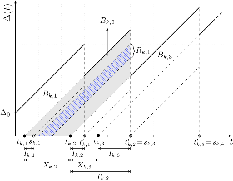
such that the area under Δk(t)subscriptΔ𝑘𝑡\Delta_{k}(t) is the sum of the disjoint areas Bk,isubscript𝐵𝑘𝑖B_{k,i}, where i=1,2,,𝒩k(τ)𝑖12subscript𝒩𝑘𝜏i\!=\!1,2,\ldots,\mathcal{N}_{k}(\tau), as shown in Figure 2. Assuming that the random process {Bk,i}subscript𝐵𝑘𝑖\{B_{k,i}\} is mean ergodic, the AAoI of sksubscript𝑠𝑘s_{k}, defined as ΔklimτΔτ,ksubscriptΔ𝑘subscript𝜏subscriptΔ𝜏𝑘\Delta_{k}\triangleq\lim_{\tau\rightarrow\infty}\Delta_{\tau,k}, converges to the stochastic average [8]. Thus, we have Δk=λk𝔼[Bk,i]subscriptΔ𝑘subscript𝜆𝑘𝔼subscript𝐵𝑘𝑖\Delta_{k}\!=\!\lambda_{k}\operatorname{\mathbb{E}}[B_{k,i}].

Refer to caption
Figure 2: AoI evolution of sksubscript𝑠𝑘s_{k} packets with respect to time t𝑡t. The blue strip highlights the server repair time while processing packet 1 from sksubscript𝑠𝑘s_{k}.

The RV Xk,i=tk,itk,i1subscript𝑋𝑘𝑖subscript𝑡𝑘𝑖subscript𝑡𝑘𝑖1X_{k,i}\!=\!t_{k,i}\!-\!t_{k,i-1} depicted in Figure 2 marks the i𝑖i-th inter-arrival time of sksubscript𝑠𝑘s_{k}, sk,isubscript𝑠𝑘𝑖s_{k,i} denotes the instant at which the transmission of the (k,i)𝑘𝑖(k,i)-th packet commences, Ik,i=sk,itk,isubscript𝐼𝑘𝑖subscript𝑠𝑘𝑖subscript𝑡𝑘𝑖I_{k,i}\!=\!s_{k,i}\!-\!t_{k,i} is the i𝑖i-th idle time of the server for source sksubscript𝑠𝑘s_{k}, and the system sojourn time is denoted by RV Tk,i=tk,itk,isubscript𝑇𝑘𝑖subscriptsuperscript𝑡𝑘𝑖subscript𝑡𝑘𝑖T_{k,i}\!=\!t^{\prime}_{k,i}\!-\!t_{k,i}. In a classical queueing model, the transmission of the (k,i1)𝑘𝑖1(k,i-1)-th packet completes at the same time as the transmission of the (k,i)𝑘𝑖(k,i)-th packet begins only if the packet generated at instant tk,isubscript𝑡𝑘𝑖t_{k,i} lies within the interval (sk,i1,tk,i1)subscript𝑠𝑘𝑖1subscriptsuperscript𝑡𝑘𝑖1(s_{k,i-1},t^{\prime}_{k,i-1}). During the transmission period, however, the server is subject to active breakdowns. The repair process begins as soon as the server fails. In such a case, the packet being served before the server breakdown resumes its remaining service immediately after the server is repaired. Hence, Tk,isubscript𝑇𝑘𝑖T_{k,i} is the system time of packet (k,i)𝑘𝑖(k,i), i.e., the sum of the packet waiting time (Wk,i)subscript𝑊𝑘𝑖(W_{k,i}) and the service time (Sk,i)subscript𝑆𝑘𝑖(S_{k,i}) which itself, includes the possible repair time when the system fails (Rk,i)subscript𝑅𝑘𝑖(R_{k,i}). Undertaking the approach in [8], the AAoI of source sksubscript𝑠𝑘s_{k} is determined to be:

ΔksubscriptΔ𝑘\displaystyle\Delta_{k} =λk𝔼[Bk,i]=λk(12𝔼[(Xk,i+Tk,i)2]12𝔼[Xk,i2])absentsubscript𝜆𝑘𝔼subscript𝐵𝑘𝑖subscript𝜆𝑘12𝔼superscriptsubscript𝑋𝑘𝑖subscript𝑇𝑘𝑖212𝔼subscriptsuperscript𝑋2𝑘𝑖\displaystyle\!=\!\lambda_{k}\operatorname{\mathbb{E}}[B_{k,i}]\!=\!\lambda_{k}\left(\frac{1}{2}\operatorname{\mathbb{E}}\left[(X_{k,i}+T_{k,i})^{2}\right]\!-\!\frac{1}{2}\operatorname{\mathbb{E}}\left[X^{2}_{k,i}\right]\right)
=λk(𝔼[Xk,i2]2+𝔼[Xk,i(Wk,i+Sk,i)]).absentsubscript𝜆𝑘𝔼subscriptsuperscript𝑋2𝑘𝑖2𝔼subscript𝑋𝑘𝑖subscript𝑊𝑘𝑖subscript𝑆𝑘𝑖\displaystyle\!=\!\lambda_{k}\left(\frac{\operatorname{\mathbb{E}}[X^{2}_{k,i}]}{2}+\operatorname{\mathbb{E}}\left[X_{k,i}(W_{k,i}+S_{k,i})\right]\right).\vspace{-0.5em} (3)

III Single-Source Unreliable M/G/1 Queue: Steady-State Distribution

On breaking down while processing a update packet, the server in an M/G/1 queue instantly undergoes repair, which has a generally distributed time. Without loss of generality, we assume that the single source, s1subscript𝑠1s_{1}, generates packets at rate λ1>0subscript𝜆10\lambda_{1}\!>\!0. We use S(t)superscript𝑆𝑡S^{\circ}(t) and R(t)superscript𝑅𝑡R^{\circ}(t) to denote the remaining packet service and server repair times, respectively, at t0𝑡0t\geq 0. If M(t)𝑀𝑡M(t) is the total of packets in the queue at time t𝑡t, then the server state can be defined as:

C(t)={0, if the server is idle,1, if the server is serving a packet,2, if the server fails while serving a packet,𝐶𝑡cases0 if the server is idle1 if the server is serving a packet2 if the server fails while serving a packetC(t)=\begin{cases}0,&\text{ if the server is {idle}},\vspace{-0.25em}\\ 1,&\text{ if the server is {serving a packet}},\vspace{-0.25em}\\ 2,&\text{ if the server {fails while serving a packet}},\end{cases}\vspace{-0.2em} (4)

For generally distributed service and repair times, the following continuous-time Markov chain captures the system state at t𝑡t:

K(t)={(C(t),M(t),S(t),R(t));t0}.𝐾𝑡𝐶𝑡𝑀𝑡superscript𝑆𝑡superscript𝑅𝑡𝑡0K(t)=\{\left(C(t),M(t),S^{\circ}(t),R^{\circ}(t)\right);t\geq 0\}.\vspace{-0.3em} (5)

Based on (5), the state probabilities are defined as follows, where m,x,y0𝑚𝑥𝑦0m,x,y\geq 0:

{p0(t)=Pr[C(t)=0,M(t)=0],p1m(x,t)dx=Pr[C(t)=1,M(t)=m,x<S(t)x+dx],p2m(x,y,t)dy=Pr[C(t)=2,M(t)=m,S(t)=x,y<R(t)y+dy],\begin{cases}p_{0}(t)=\Pr[C(t)=0,M(t)=0],\vspace{-0.1em}\\ p_{1}^{m}(x,t)\,\text{d}x=\Pr[C(t)\!=\!1,M(t)\!=\!m,x<\!S^{\circ}(t)\!\leq\!x+\text{d}x],\vspace{-0.1em}\\ p_{2}^{m}(x,y,t)\text{d}y=\Pr[C(t)\!=\!2,M(t)\!=\!m,S^{\circ}(t)=x,\\ \qquad\qquad\qquad\qquad\qquad\qquad\qquad y<R^{\circ}(t)\leq y+\text{d}y],\end{cases}\vspace{-0.2em} (6)

where p0(t)subscript𝑝0𝑡p_{0}(t) denotes the probability that the server is idle at time t𝑡t, p1m(x,t)dxsuperscriptsubscript𝑝1𝑚𝑥𝑡d𝑥p_{1}^{m}(x,t)\,\text{d}x refers to the joint probability that the server is busy transmitting a packet during the remaining service time (x,x+dx)𝑥𝑥d𝑥(x,x+\text{d}x) while there are m𝑚m packets in the queue at time t𝑡t, p2m(x,y,t)dysuperscriptsubscript𝑝2𝑚𝑥𝑦𝑡d𝑦p_{2}^{m}(x,y,t)\,\text{d}y refers to the joint probability that there are m𝑚m queued packets, the remaining service time is x𝑥x, and the failed server is fixed within the remaining repair time (y,y+dy)𝑦𝑦d𝑦(y,y\!+\!\text{d}y) while serving a packet.

We now apply the method of supplementary variables [13] to obtain the following balance equations from (6) as t𝑡t\rightarrow\infty:

{λ1p0=p10(0),\diffp10(x)x=(λ1+α)p10(x)(λ1p0+p11(0))fs(x)p20(x,0),\diffp1m(x)x=(λ1+α)p1m(x)λ1p1m1(x)p1m+1(0)fs(x)p2m(x,0),\diffpp2m(x,y)y=λ1p2m(x,y)λ1p2m1(x,y)αp1m(x)fr(y),casessubscript𝜆1subscript𝑝0superscriptsubscript𝑝100otherwise\diffsuperscriptsubscript𝑝10𝑥𝑥subscript𝜆1𝛼superscriptsubscript𝑝10𝑥subscript𝜆1subscript𝑝0superscriptsubscript𝑝110subscript𝑓𝑠𝑥superscriptsubscript𝑝20𝑥0otherwise\diffsuperscriptsubscript𝑝1𝑚𝑥𝑥subscript𝜆1𝛼superscriptsubscript𝑝1𝑚𝑥subscript𝜆1superscriptsubscript𝑝1𝑚1𝑥superscriptsubscript𝑝1𝑚10subscript𝑓𝑠𝑥superscriptsubscript𝑝2𝑚𝑥0otherwise\diffpsuperscriptsubscript𝑝2𝑚𝑥𝑦𝑦subscript𝜆1superscriptsubscript𝑝2𝑚𝑥𝑦subscript𝜆1superscriptsubscript𝑝2𝑚1𝑥𝑦𝛼superscriptsubscript𝑝1𝑚𝑥subscript𝑓𝑟𝑦otherwise\begin{cases}\!\lambda_{1}p_{0}=p_{1}^{0}(0),\vspace{0.3em}\\ \!\diff{p_{1}^{0}(x)}{x}\!=\!(\lambda_{1}\!+\!\alpha)p_{1}^{0}(x)\!-\!\left(\lambda_{1}p_{0}\!+\!p_{1}^{1}(0)\right)\!f_{s}(x)\!-\!p_{2}^{0}(x,0),\vspace{0.3em}\\ \!\diff{p_{1}^{m\!}(x)\!}{x}\!=\!(\!\lambda_{1\!}\!+\!\alpha\!)p_{1}^{m\!}(x)\!-\!\!\lambda_{1}p_{1}^{m\!-\!1\!}(x)\!-\!p_{1}^{m\!+\!1\!}(0)f_{\!s}(x)\!-\!p_{2}^{m\!}(x,\!0),\vspace{0.3em}\\ \!\diffp{p_{2}^{m\!}(x,y)}{y}\!=\!\lambda_{1}p_{2}^{m}(x,y)\!-\!\lambda_{1}p_{2}^{m\!-\!1}(x,y)-\alpha p_{1}^{m}(x)f_{r}(y),\end{cases}\vspace{-0.2em} (7)

where fs(x)subscript𝑓𝑠𝑥f_{s}(x) and fr(x)subscript𝑓𝑟𝑥f_{r}(x) are, respectively, the probability density functions of the service and repair times, and the normalization condition is given as:

p0+m=0[0p1m(x)dx+00p2m(x,y)dxdy]=1.subscript𝑝0superscriptsubscript𝑚0delimited-[]superscriptsubscript0superscriptsubscript𝑝1𝑚𝑥d𝑥superscriptsubscript0superscriptsubscript0superscriptsubscript𝑝2𝑚𝑥𝑦d𝑥d𝑦1p_{0}+\sum_{m=0}^{\infty}\left[\int_{0}^{\infty}\!p_{1}^{m}(x)\,\text{d}x+\int_{0}^{\infty}\!\!\int_{0}^{\infty}\!p_{2}^{m}(x,y)\,\text{d}x\,\text{d}y\right]\!=\!1.\vspace{-0.3em} (8)

Denoting the LSTs of p1m(x)superscriptsubscript𝑝1𝑚𝑥p_{1}^{m}(x) and LST[p2m(x,y)]delimited-[]superscriptsubscript𝑝2𝑚𝑥𝑦[p_{2}^{m}(x,y)] by p~1m(θ)superscriptsubscript~𝑝1𝑚𝜃\tilde{p}_{1}^{\,m}(\theta) and p~~2m(θ,s)superscriptsubscript~~𝑝2𝑚𝜃𝑠\widetilde{\tilde{p}}_{2}^{\,m}(\theta,s), respectively, the marginal pdfs are:

{p~1(z,θ)=m=0p~1m(θ)zm,p1(z,0)=m=0p1m(0)zm,p~~2(z,θ,s)=m=0p~~2m(θ,s)zm,p~2(z,θ,0)=m=0p~2m(θ,0)zm,casessubscript~𝑝1𝑧𝜃superscriptsubscript𝑚0superscriptsubscript~𝑝1𝑚𝜃superscript𝑧𝑚otherwisesubscript𝑝1𝑧0superscriptsubscript𝑚0superscriptsubscript𝑝1𝑚0superscript𝑧𝑚otherwisesubscript~~𝑝2𝑧𝜃𝑠superscriptsubscript𝑚0superscriptsubscript~~𝑝2𝑚𝜃𝑠superscript𝑧𝑚otherwisesubscript~𝑝2𝑧𝜃0superscriptsubscript𝑚0superscriptsubscript~𝑝2𝑚𝜃0superscript𝑧𝑚otherwise\begin{cases}\tilde{p}_{1}(z,\theta)=\sum_{m=0}^{\infty}\tilde{p}_{1}^{\,m}(\theta)z^{m},\vspace{0.3em}\\ p_{1}(z,0)=\sum_{m=0}^{\infty}p_{1}^{m}(0)z^{m},\vspace{0.3em}\\ \widetilde{\tilde{p}}_{2}(z,\theta,s)=\sum_{m=0}^{\infty}\widetilde{\tilde{p}}_{2}^{\,m}(\theta,s)z^{m},\vspace{0.3em}\\ \tilde{p}_{2}(z,\theta,0)=\sum_{m=0}^{\infty}\tilde{p}_{2}^{\,m}(\theta,0)z^{m},\end{cases}\vspace{-0.3em} (9)

By applying LST on both sides of (7), multiplying zmsuperscript𝑧𝑚z^{m} to the resultant equations, summing over m𝑚m, and through some algebraic manipulations, the pgfs of the queue size, 𝒫(z)𝒫𝑧\mathcal{P}(z), and the system size, 𝒬(z)𝒬𝑧\mathcal{Q}(z), are derived to be as follows, where p0=1λ1β(1,1)(1+αγ(1,1))subscript𝑝01subscript𝜆1superscript𝛽111𝛼superscript𝛾11p_{0}\!=\!1\!-\!\lambda_{1}\beta^{(1,1)}(1\!+\!\alpha\gamma^{(1,1)}) and ϕ(s,z)=(s+λ1λ1z+ααR(s+λ1λ1z))italic-ϕ𝑠𝑧𝑠subscript𝜆1subscript𝜆1𝑧𝛼𝛼superscript𝑅𝑠subscript𝜆1subscript𝜆1𝑧\phi(s,z)\!=\!\left(s\!+\!\lambda_{1}\!-\!\lambda_{1}z\!+\!\alpha\!-\!\alpha R^{*}(s\!+\!\lambda_{1}\!-\!\lambda_{1}z)\right):

{𝒫(z)=p0+p~1(z,0)+p~~2(z,0,0)=(1S(ϕ(0,z)))p0S(ϕ(0,z))z,𝒬(z)=p0+zp~1(z,0)+zp~~2(z,0,0)=S(ϕ(0,z))(1z)p0S(ϕ(0,z))z,cases𝒫𝑧subscript𝑝0subscript~𝑝1𝑧0subscript~~𝑝2𝑧001superscript𝑆italic-ϕ0𝑧subscript𝑝0superscript𝑆italic-ϕ0𝑧𝑧otherwise𝒬𝑧subscript𝑝0𝑧subscript~𝑝1𝑧0𝑧subscript~~𝑝2𝑧00superscript𝑆italic-ϕ0𝑧1𝑧subscript𝑝0superscript𝑆italic-ϕ0𝑧𝑧otherwise\begin{cases}\!\!\mathcal{P}(z)\!=\!p_{0}\!+\!\tilde{p}_{1}(z,\!0)\!+\!\widetilde{\tilde{p}}_{2}(z,\!0,\!0)\!=\!\dfrac{\left(1\!-\!S^{*}\!\left(\phi(0,\!z)\right)\right)p_{0}}{S^{*}\!\left(\phi(0,\!z)\right)\!-\!z},\vspace{0.3em}\\ \!\!\mathcal{Q}(z)\!=\!p_{0}\!+\!z\tilde{p}_{1}(z,\!0)\!+\!z\widetilde{\tilde{p}}_{2}(z,\!0,\!0)\!=\!\dfrac{S^{*}\!\left(\phi(0,\!z)\right)\!(1\!-\!z)p_{0}}{S^{*}\!\left(\phi(0,\!z)\right)\!-\!z},\end{cases}\vspace{-0.2em} (10)

To obtain the LST of sojourn time distribution of the system, we substitute a=λ1(1z)𝑎subscript𝜆11𝑧a\!=\!\lambda_{1}(1-z) in 𝒬(z)𝒬𝑧\mathcal{Q}(z) given in (10):

W(a)=a(S(a+α(1R(a))))p0(aλ1(1S(a+α(1R(a))))).superscript𝑊𝑎𝑎superscript𝑆𝑎𝛼1superscript𝑅𝑎subscript𝑝0𝑎subscript𝜆11superscript𝑆𝑎𝛼1superscript𝑅𝑎W^{*}(a)=\dfrac{a\left(S^{*}\!\left(a+\alpha\left(1-R^{*}(a)\right)\right)\right)p_{0}}{\left(a-\lambda_{1}\left(1-S^{*}(a+\alpha\left(1-R^{*}(a)\right))\right)\right)}.\vspace{-0.2em} (11)

The system availability at time t𝑡t, denoted by A(t)𝐴𝑡A(t), determines the likelihood of when the unreliable server will be available for use. In steady-state, i.e., Pa=limtA(t)subscript𝑃𝑎subscript𝑡𝐴𝑡P_{a}=\lim_{t\to\infty}A(t), we get:

Pa=limz1{p0+p~1(z,0)}=1λ1β(1,1)αγ(1,1).subscript𝑃𝑎subscript𝑧1subscript𝑝0subscript~𝑝1𝑧01subscript𝜆1superscript𝛽11𝛼superscript𝛾11P_{a}=\lim_{z\to 1}\{p_{0}+\tilde{p}_{1}(z,0)\}\!=\!1-\lambda_{1}\beta^{(1,1)}\alpha\gamma^{(1,1)}.\vspace{-0.4em} (12)

IV Multi-Source Unreliable M/G/1 Queue: AoI Analysis

In this section, we derive the AAoI defined in (3) for the unreliable M/G/1 queueing model with multiple sources. We begin our analysis of (3) by considering sources s1subscript𝑠1s_{1} and s2subscript𝑠2s_{2}. For the first term in (3), we have 𝔼[X1,i2]=2/λ12𝔼subscriptsuperscript𝑋21𝑖2superscriptsubscript𝜆12\operatorname{\mathbb{E}}[X^{2}_{1,i}]\!=\!2/\lambda_{1}^{2} since the inter-arrival time of s1subscript𝑠1s_{1} follows an exponential distribution with λ1>0subscript𝜆10\lambda_{1}\!>\!0. The second term in (3) can be expressed as follows:

𝔼[X1,i(W1,i+S1,i)]=𝔼[X1,iW1,i]+𝔼[X1,i]𝔼[S1,i].𝔼subscript𝑋1𝑖subscript𝑊1𝑖subscript𝑆1𝑖𝔼subscript𝑋1𝑖subscript𝑊1𝑖𝔼subscript𝑋1𝑖𝔼subscript𝑆1𝑖\operatorname{\mathbb{E}}[X_{1,i}(W_{1,i}+S_{1,i})]=\operatorname{\mathbb{E}}[X_{1,i}W_{1,i}]+\operatorname{\mathbb{E}}[X_{1,i}]\operatorname{\mathbb{E}}[S_{1,i}].\vspace{-0.2em} (13)

In (13), the second term arises as the inter-arrival time and service time (including the repair time) are independent of each other. However, evaluation of the first term in (13) is computationally complex since the inter-arrival and waiting times are dependent. To find 𝔼[X1,iW1,i]𝔼subscript𝑋1𝑖subscript𝑊1𝑖\operatorname{\mathbb{E}}[X_{\!1,i}W_{1,i}], we express W1,isubscript𝑊1𝑖W_{1,i} in terms of two events, namely A1,ibsubscriptsuperscript𝐴𝑏1𝑖A^{b}_{1,i} and A1,ilsubscriptsuperscript𝐴𝑙1𝑖A^{l}_{1,i}. The former represents the event when the inter-arrival time of packet (1,i)1𝑖(1,i) is shorter than the system time of packet (1,i1)1𝑖1(1,i\!-\!1), whereas the latter is the complementary event. Under event A1,ibsubscriptsuperscript𝐴𝑏1𝑖A^{b}_{1,i}, the waiting time of packet (1,i)1𝑖(1,i) comprises of (i) the remaining time to complete processing packet (1,i1)1𝑖1(1,i\!-\!1), (ii) the sum of service times of s2subscript𝑠2s_{2} packets that arrived during X1,isubscript𝑋1𝑖X_{1,i} and must be served before packet (1,i)1𝑖(1,i) according to the FCFS rule, and (iii) the sum of possible server repair times before serving packet (1,i)1𝑖(1,i). Similarly, for A1,ilsubscriptsuperscript𝐴𝑙1𝑖A^{l}_{1,i}, the waiting time of packet (1,i)1𝑖(1,i) includes (i) the remaining service time of s2subscript𝑠2s_{2} packet under service at the instant packet (1,i)1𝑖(1,i) arrives, (ii) the sum of service times of s2subscript𝑠2s_{2} packets served prior to packet (1,i)1𝑖(1,i) in FCFS order, and (iii) the total repair time before processing the (1,i)1𝑖(1,i)-th packet.

For event A1,ibsubscriptsuperscript𝐴𝑏1𝑖A^{b}_{1,i}, let R1,ib=T1,i1X1,isubscriptsuperscript𝑅𝑏1𝑖subscript𝑇1𝑖1subscript𝑋1𝑖R^{b}_{1,i}\!=\!T_{1,i-1}\!-\!X_{1,i} be the residual system time to complete serving packet (1,i1)1𝑖1(1,i\!-\!1). Also, let the total service times of s2subscript𝑠2s_{2} packets arriving during X1,isubscript𝑋1𝑖X_{1,i} that need service before packet (1,i)1𝑖(1,i) be S1,ib=iΩ2,ibS2,isubscriptsuperscript𝑆𝑏1𝑖subscriptsuperscript𝑖subscriptsuperscriptΩ𝑏2𝑖subscript𝑆2superscript𝑖S^{b}_{1,i\!}\!=\!\!\sum_{i^{\prime}\in\Omega^{b}_{2,i}}\!\!S_{2,i^{\prime}}, where Ω2,ibsubscriptsuperscriptΩ𝑏2𝑖\Omega^{b}_{2,i} is the index set of queued packets from s2subscript𝑠2s_{2}. Let F1,ib=iΩ2,ibR2,isubscriptsuperscript𝐹𝑏1𝑖subscriptsuperscript𝑖subscriptsuperscriptΩ𝑏2𝑖subscript𝑅2superscript𝑖F^{b}_{1,i}\!=\!\sum_{i^{\prime}\in\Omega^{b}_{2,i}}\!\!R_{2,i^{\prime}} be the total server repair time before serving the (1,i)1𝑖(1,i)-th packet. In the same manner, we define S1,il=iΩ2,ilS2,isubscriptsuperscript𝑆𝑙1𝑖subscriptsuperscript𝑖subscriptsuperscriptΩ𝑙2𝑖subscript𝑆2superscript𝑖S^{l}_{1,i}\!=\!\sum_{i^{\prime}\in\Omega^{l}_{2,i}}\!\!S_{2,i^{\prime}} and F1,il=iΩ2,ilR2,isubscriptsuperscript𝐹𝑙1𝑖subscriptsuperscript𝑖subscriptsuperscriptΩ𝑙2𝑖subscript𝑅2superscript𝑖F^{l}_{1,i}\!=\!\sum_{i^{\prime}\in\Omega^{l}_{2,i}}\!\!R_{2,i^{\prime}} for event A1,ilsubscriptsuperscript𝐴𝑙1𝑖A^{l}_{1,i}, where Ω2,ilsubscriptsuperscriptΩ𝑙2𝑖\Omega^{l}_{2,i} is the set of indices of queued packets generated by source s2subscript𝑠2s_{2}. Using these definitions, the waiting time of packet (1,i)1𝑖(1,i) can be written as:

W1,i={S1,ib+F1,ib+R1,ib, if A1,ib occurs,S1,il+F1,il+R2,il, if A1,il occurs,subscript𝑊1𝑖casessubscriptsuperscript𝑆𝑏1𝑖subscriptsuperscript𝐹𝑏1𝑖subscriptsuperscript𝑅𝑏1𝑖 if subscriptsuperscript𝐴𝑏1𝑖 occurssubscriptsuperscript𝑆𝑙1𝑖subscriptsuperscript𝐹𝑙1𝑖subscriptsuperscript𝑅𝑙2𝑖 if subscriptsuperscript𝐴𝑙1𝑖 occursW_{1,i}=\begin{cases}S^{b}_{1,i}+F^{b}_{1,i}+R^{b}_{1,i},&\text{ if }A^{b}_{1,i}\text{ occurs},\vspace{-0.05em}\\ S^{l}_{1,i}+F^{l}_{1,i}+R^{l}_{2,i},&\text{ if }A^{l}_{1,i}\text{ occurs},\end{cases}\vspace{-0.3em} (14)

where R2,ilsubscriptsuperscript𝑅𝑙2𝑖R^{l}_{2,i} denotes the residual service time RV of the s2subscript𝑠2s_{2} packet under service at the arrival of packet (1,i)1𝑖(1,i) conditioned on event A1,ilsubscriptsuperscript𝐴𝑙1𝑖A^{l}_{1,i}. By taking the conditional expectation on (13), we get:

𝔼[X1,iW1,i]=𝔼subscript𝑋1𝑖subscript𝑊1𝑖absent\displaystyle\operatorname{\mathbb{E}}[X_{\!1,i}W_{\!1,i}]\!=\! (𝔼[R1,ibX1,i|A1,ib]+𝔼[(S1,ib+F1,ib)X1,i|A1,ib])p1,ib𝔼conditionalsubscriptsuperscript𝑅𝑏1𝑖subscript𝑋1𝑖subscriptsuperscript𝐴𝑏1𝑖𝔼conditionalsubscriptsuperscript𝑆𝑏1𝑖subscriptsuperscript𝐹𝑏1𝑖subscript𝑋1𝑖subscriptsuperscript𝐴𝑏1𝑖subscriptsuperscript𝑝𝑏1𝑖\displaystyle\left(\operatorname{\mathbb{E}}[R^{b}_{1,i}X_{\!1,i}|A^{b}_{1,i}]\!+\!\operatorname{\mathbb{E}}[(S^{b}_{1,i\!}\!+\!F^{b}_{1,i})X_{\!1\!,i}|A^{b}_{1,i}]\right)p^{b}_{1,i}
+𝔼[(S1,il+F1,il+R2,il)X1,i|A1,il]p1,il,𝔼conditionalsubscriptsuperscript𝑆𝑙1𝑖subscriptsuperscript𝐹𝑙1𝑖subscriptsuperscript𝑅𝑙2𝑖subscript𝑋1𝑖subscriptsuperscript𝐴𝑙1𝑖subscriptsuperscript𝑝𝑙1𝑖\displaystyle+\!\operatorname{\mathbb{E}}[(S^{l}_{1,i}\!+\!F^{l}_{1,i}\!+\!R^{l}_{2,i})X_{1,i}|A^{l}_{1,i}]\,p^{l}_{1,i},\vspace{-0.4em} (15)

where p1,ibsubscriptsuperscript𝑝𝑏1𝑖p^{b}_{1,i} and p1,ilsubscriptsuperscript𝑝𝑙1𝑖p^{l}_{1,i} are the probabilities of events A1,ibsubscriptsuperscript𝐴𝑏1𝑖A^{b}_{1,i} and A1,ilsubscriptsuperscript𝐴𝑙1𝑖A^{l}_{1,i}, respectively, and are derived to be:

{p1,ib=1p1,il,p1,il=S(λ1+α(1R(λ1)))λ1p0(λ1λ(1S(λ1+α(1R(λ1))))),casessubscriptsuperscript𝑝𝑏1𝑖1subscriptsuperscript𝑝𝑙1𝑖otherwisesubscriptsuperscript𝑝𝑙1𝑖superscript𝑆subscript𝜆1𝛼1superscript𝑅subscript𝜆1subscript𝜆1subscript𝑝0subscript𝜆1𝜆1superscript𝑆subscript𝜆1𝛼1superscript𝑅subscript𝜆1otherwise\begin{cases}p^{b}_{1,i}=1-p^{l}_{1,i},\vspace{0.15em}\\ p^{l}_{1,i}=\dfrac{S^{*}\big{(}\lambda_{1}\!+\!\alpha\left(1-R^{*}(\lambda_{1})\right)\!\big{)}\lambda_{1}p_{0}}{\big{(}\lambda_{1}\!-\!\lambda\left(1\!-\!S^{*}\!\left(\lambda_{1}\!+\!\alpha\left(1-R^{*}(\lambda_{1})\right)\right)\right)\!\big{)}},\end{cases}\vspace{-0.4em} (16)

where λ=kλk𝜆subscript𝑘subscript𝜆𝑘\lambda\!=\!\sum_{k}\lambda_{k}, and the service and sojourn times of all packets are stochastically identical, i.e., ifor-all𝑖\forall i and k=1,2,,N𝑘12𝑁k\!=\!1,2,\ldots,N, we have Sk,i=Ssubscript𝑆𝑘𝑖𝑆S_{k,i}\!=\!S and Tk,i=Tsubscript𝑇𝑘𝑖𝑇T_{k,i}\!=\!T. For the sake of presentation, we substitute G1,ib=S1,ib+F1,ibsubscriptsuperscript𝐺𝑏1𝑖subscriptsuperscript𝑆𝑏1𝑖subscriptsuperscript𝐹𝑏1𝑖G^{b}_{1,i}\!=\!S^{b}_{1,i}\!+\!F^{b}_{1,i} and G1,il=S1,il+F1,ilsubscriptsuperscript𝐺𝑙1𝑖subscriptsuperscript𝑆𝑙1𝑖subscriptsuperscript𝐹𝑙1𝑖G^{l}_{1,i}\!=\!S^{l}_{1,i}\!+\!F^{l}_{1,i} in (15). From probability theory, the conditional probability density function of RVs X1,isubscript𝑋1𝑖X_{1,i} and T1,i1subscript𝑇1𝑖1T_{1,i-1}, given the event A1,ibsubscriptsuperscript𝐴𝑏1𝑖A^{b}_{1,i}, can be expressed as:

fX1,i,T1,i1|A1,ib(s,t)={λ1eλ1sfT1,i1(t)p1,ib, if st,0, if s>t.subscript𝑓subscript𝑋1𝑖conditionalsubscript𝑇1𝑖1subscriptsuperscript𝐴𝑏1𝑖𝑠𝑡casessubscript𝜆1superscript𝑒subscript𝜆1𝑠subscript𝑓subscript𝑇1𝑖1𝑡subscriptsuperscript𝑝𝑏1𝑖 if 𝑠𝑡0 if 𝑠𝑡f_{X_{1,i},T_{1,i-1}|A^{b}_{1,i}\!}(s,t)\!=\!\begin{cases}\!\dfrac{\lambda_{1}e^{-\lambda_{1}s}f_{T_{1,i-1}}(t)}{p^{b}_{1,i}},&\text{ if }s\leq t,\vspace{0.03em}\\ \!0,&\text{ if }s>t.\end{cases}\vspace{-0.3em} (17)

Using (17), we derive the three conditional expressions of (15) in Lemmas 1-3, where kfor-all𝑘\forall k, we assume ρk=λkβ(1,1)(1+αγ(1,1))subscript𝜌𝑘subscript𝜆𝑘superscript𝛽111𝛼superscript𝛾11\rho_{k}\!=\!\lambda_{k}\beta^{(1,1)}(1\!+\!\alpha\gamma^{(1,1)}).

Lemma 1.

The closed-form expression for the first conditional expectation in (15) is given as:

𝔼[R1,ibX1,i|A1,ib]=1λ1p1,ib(𝔼[W]+𝔼[S]W(λ1)+2W(λ1)2λ1).𝔼conditionalsubscriptsuperscript𝑅𝑏1𝑖subscript𝑋1𝑖subscriptsuperscript𝐴𝑏1𝑖1subscript𝜆1subscriptsuperscript𝑝𝑏1𝑖𝔼𝑊𝔼𝑆superscript𝑊superscriptsubscript𝜆12superscript𝑊subscript𝜆12subscript𝜆1\operatorname{\mathbb{E}}[R^{b}_{1\!,i}X_{\!1\!,i}|A^{b}_{1\!,i}]\!=\!\!\dfrac{1}{\lambda_{1}p^{b}_{1,i}\!\!}\!\!\left(\!\operatorname{\mathbb{E}}[W\!]\!+\!\operatorname{\mathbb{E}}[S]\!-\!\!W^{*^{\prime}\!}\!(\!\lambda_{1\!})\!+\!\dfrac{2W^{*\!}(\lambda_{1\!})\!-\!\!2}{\lambda_{1}}\!\right)\!.\vspace{-0.4em} (18)
Proof.

See Appendix A. ∎

Lemma 2.

The closed-form expression for the second conditional expectation in (15) is given as:

𝔼[G1,ibX1,i|A1,ib]=ρ2p1,ib(2λ12W′′(λ1)+2W(λ1)λ1+2W(λ1)λ12).𝔼conditionalsubscriptsuperscript𝐺𝑏1𝑖subscript𝑋1𝑖subscriptsuperscript𝐴𝑏1𝑖subscript𝜌2subscriptsuperscript𝑝𝑏1𝑖2superscriptsubscript𝜆12superscript𝑊superscript′′subscript𝜆12superscript𝑊superscriptsubscript𝜆1subscript𝜆12superscript𝑊subscript𝜆1superscriptsubscript𝜆12\operatorname{\mathbb{E}}[G^{b}_{1\!,i}X_{\!1\!,i}|A^{b}_{1\!,i}]\!=\!\!\dfrac{\rho_{2}}{p^{b}_{1,i}\!\!}\!\left(\!\!\dfrac{2}{\lambda_{1}^{2}}\!-\!W^{*^{\prime\prime}\!\!}(\lambda_{1\!})\!+\!\!\dfrac{2W^{*^{\prime}\!}(\lambda_{1\!})}{\lambda_{1}}\!+\!\dfrac{2W^{*\!}(\!\lambda_{1\!})}{\lambda_{1}^{2}}\!\right)\!.\vspace{-0.4em} (19)
Proof.

See Appendix B. ∎

Lemma 3.

The closed-form expression for the third conditional expectation in (15) is given as:

𝔼[(G1,il+R2,il)X1,i|A1,il]=ρ2p1,il(W′′(λ1)W(λ1)λ1).𝔼conditionalsubscriptsuperscript𝐺𝑙1𝑖subscriptsuperscript𝑅𝑙2𝑖subscript𝑋1𝑖subscriptsuperscript𝐴𝑙1𝑖subscript𝜌2subscriptsuperscript𝑝𝑙1𝑖superscript𝑊superscript′′subscript𝜆1superscript𝑊superscriptsubscript𝜆1subscript𝜆1\operatorname{\mathbb{E}}[\left(G^{l}_{1\!,i}\!+\!R^{l}_{2,i}\right)X_{\!1\!,i}|A^{l}_{1\!,i}]=\dfrac{\rho_{2}}{p^{l}_{1,i}}\!\left(\!W^{*^{\prime\prime}\!\!}(\lambda_{1})\!-\!\!\dfrac{W^{*^{\prime}\!}(\lambda_{1})}{\lambda_{1}}\!\right)\!.\vspace{-0.3em} (20)
Proof.

See Appendix C. ∎

Refer to caption
Refer to caption
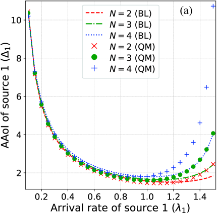
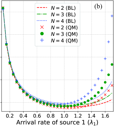
Figure 3: The AAoI of source s1subscript𝑠1s_{1} in terms of λ1subscript𝜆1\lambda_{1} for N={2,3,4}𝑁234N\!=\!\{2,3,4\} under (a) Erlang-222 and (b) hyper-exponential service time distributions with p=0.7𝑝0.7p\!=\!0.7. Here, 𝔼[S]=0.5𝔼𝑆0.5\operatorname{\mathbb{E}}[S]=0.5, 𝔼[R]=0.3𝔼𝑅0.3\operatorname{\mathbb{E}}[R]=0.3, α=0.1𝛼0.1\alpha=0.1, and λi(i1)=0.12subscript𝜆𝑖𝑖10.12\lambda_{i}(i\neq 1)\!=\!0.12.

From (18)-(20), the AAoI of source s1subscript𝑠1s_{1} in a two-source unreliable M/G/1 queueing model can be computed as follows:

Δ1=𝔼[W]+2𝔼[S]+2ρ21λ1+2(1ρ2)W(λ1)λ1+(ρ21)W(λ1).subscriptΔ1𝔼𝑊2𝔼𝑆2subscript𝜌21subscript𝜆121subscript𝜌2superscript𝑊subscript𝜆1subscript𝜆1subscript𝜌21superscript𝑊superscriptsubscript𝜆1\Delta_{1\!}\!=\!\operatorname{\mathbb{E}}[W]+2\!\operatorname{\mathbb{E}}[S]+\dfrac{2\rho_{2\!}\!-\!\!1}{\lambda_{1}}+\dfrac{2(\!1\!\!-\!\!\rho_{2}\!)W^{*\!}(\lambda_{1\!})}{\lambda_{1}}+(\rho_{2}-\!1\!)W^{*^{\prime}\!\!}(\lambda_{1}\!).\vspace{-0.3em} (21)

In general, the AAoI of source s1subscript𝑠1s_{1} in a multi-source M/G/1 model with server breakdowns can be calculated by replacing ρ2subscript𝜌2\rho_{2} in (21) with j𝒮/{1}ρjsubscript𝑗𝒮1subscript𝜌𝑗\sum_{j\in\mathcal{S}/\{1\}}\rho_{j} as follows:

Δ1=subscriptΔ1absent\displaystyle\Delta_{1}= 𝔼[W]+2𝔼[S]+2W(λ1)λ1W(λ1)1λ1𝔼𝑊2𝔼𝑆2superscript𝑊subscript𝜆1subscript𝜆1superscript𝑊superscriptsubscript𝜆11subscript𝜆1\displaystyle\operatorname{\mathbb{E}}[W]+2\operatorname{\mathbb{E}}[S]+\dfrac{2W^{*}(\lambda_{1})}{\lambda_{1}}-W^{*^{\prime}}(\lambda_{1})-\dfrac{1}{\lambda_{1}}
+j𝒮/{1}ρj(2λj+W(λj)2W(λj)λj).subscript𝑗𝒮1subscript𝜌𝑗2subscript𝜆𝑗superscript𝑊superscriptsubscript𝜆𝑗2superscript𝑊subscript𝜆𝑗subscript𝜆𝑗\displaystyle+\sum_{j\in\mathcal{S}/\{1\}}\rho_{j}\left(\dfrac{2}{\lambda_{j}}+W^{*^{\prime}}(\lambda_{j})-\dfrac{2W^{*}(\lambda_{j})}{\lambda_{j}}\right).\vspace{-1.9em} (22)

V Numerical Results and Discussions

In this section, we evaluate the AAoI in a multi-source unreliable M/G/1 queueing model (QM) and compare our analytical findings with the multi-source M/G/1 baseline model (BL) studied in [8]. For this purpose, we consider Erlang-2 (Erl.) and hyper-exponential of order 2 (H2subscript𝐻2H_{2}) service time distributions. The probability density function corresponding to the H2subscript𝐻2H_{2} distribution is given as follows, where γ1=2p/m1subscript𝛾12𝑝subscript𝑚1\gamma_{1}\!=\!2p/m_{1}, γ2=2(1p)/m1subscript𝛾221𝑝subscript𝑚1\gamma_{2}\!=\!2(1-p)/m_{1}, p=(1+(c21)/(c2+1))/2𝑝1superscript𝑐21superscript𝑐212p\!=\!(1\!+\sqrt{(c^{2}\!-\!1)/(c^{2}\!+\!1)})/2, c21superscript𝑐21c^{2}\!\geq\!1 is the squared coefficient of variation, and m1subscript𝑚1m_{1} is the mean:

fH2(t)=pγ1eγ1t+(1p)γ2eγ2t,t0.formulae-sequencesubscript𝑓subscript𝐻2𝑡𝑝subscript𝛾1superscript𝑒subscript𝛾1𝑡1𝑝subscript𝛾2superscript𝑒subscript𝛾2𝑡𝑡0\displaystyle f_{H_{2}}(t)=p\gamma_{1}e^{-\gamma_{1}t}+(1-p)\gamma_{2}e^{-\gamma_{2}t},\quad t\!\geq\!0.\vspace{-0.4em} (23)

Figure 3 shows the AAoI of source s1subscript𝑠1s_{1} (Δ1)subscriptΔ1(\Delta_{1}) impacted by the packet arrival rate of s1subscript𝑠1s_{1} (λ1)subscript𝜆1(\lambda_{1}) under general service time distribution for varying N𝑁N values. For parameters 𝔼[S]=0.5𝔼𝑆0.5\operatorname{\mathbb{E}}[S]\!=\!0.5, 𝔼[R]=0.3𝔼𝑅0.3\operatorname{\mathbb{E}}[R]\!=\!0.3, α=0.1𝛼0.1\alpha\!=\!0.1, p=0.7𝑝0.7p\!=\!0.7, and λi(i1)=0.12subscript𝜆𝑖𝑖10.12\lambda_{i}(i\!\neq\!1)\!=\!0.12, we observe that the waiting time of packets from all sources increases with λ1subscript𝜆1\lambda_{1}, which in turn, causes Δ1subscriptΔ1\Delta_{1} to increase as well. Nonetheless, for larger λ1subscript𝜆1\lambda_{1} values, QM results in higher Δ1subscriptΔ1\Delta_{1} as compared to BL. This clearly reveals the impact of average server repair time, which is related to the expected service time as 𝔼[S]=β(1,1)(1+α𝔼[R])𝔼𝑆superscript𝛽111𝛼𝔼𝑅\operatorname{\mathbb{E}}[S]\!=\!\beta^{(1,1)}(1\!+\!\alpha\operatorname{\mathbb{E}}[R]). We also see a substantial increase in the AAoI gap between QM and BL as N𝑁N goes from 2 to 4 under all three service time distributions in Fig. 3a and Fig. 3b. Such behavior is anticipated as the unreliable server becomes overloaded with packets arriving from a larger set of sources, thus further delaying the packet processing time.
Refer to caption

Refer to caption

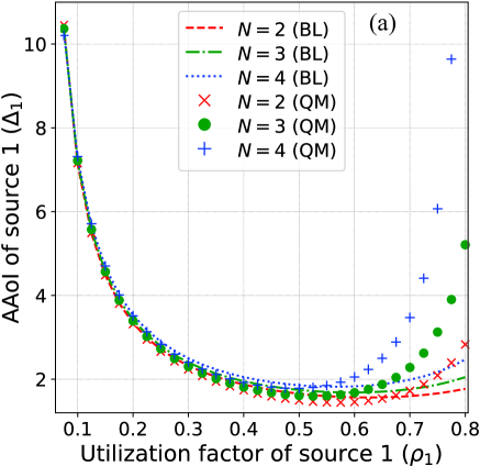
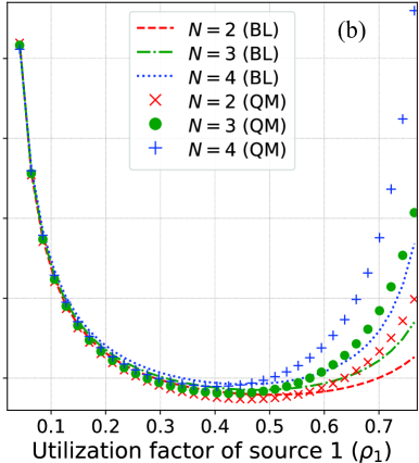
Figure 4: The AAoI of source s1subscript𝑠1s_{1} in terms of ρ1subscript𝜌1\rho_{1} for N={2,3,4}𝑁234N\!=\!\{2,3,4\} under (a) Erlang-2 and (b) hyper-exponential service time distributions with p=0.7𝑝0.7p\!=\!0.7. Here, 𝔼[S]=0.5𝔼𝑆0.5\operatorname{\mathbb{E}}[S]=0.5 and 𝔼[R]=0.3𝔼𝑅0.3\operatorname{\mathbb{E}}[R]=0.3, α=0.1𝛼0.1\alpha=0.1, and λi(i1)=0.12subscript𝜆𝑖𝑖10.12\lambda_{i}(i\neq 1)\!=\!0.12.

The effect of the traffic intensity of source 1 (ρ1=λ1𝔼[S])subscript𝜌1subscript𝜆1𝔼𝑆(\rho_{1}\!=\!\lambda_{1}\operatorname{\mathbb{E}}[S]) on Δ1subscriptΔ1\Delta_{1} is depicted in Figure 4. For the same parametric settings as in Figure 3, we note insignificant difference in the AAoI of s1subscript𝑠1s_{1} under light traffic conditions. However, as more packets arrive at the server from multiple sources, the AAoI of s1subscript𝑠1s_{1} grows non-linearly as evident in Fig. 4a and Fig. 4b. Moreover, as ρ1subscript𝜌1\rho_{1} increases, Δ1subscriptΔ1\Delta_{1} in QM rises at a much faster rate than BL. This is mainly because the packets being processed are interrupted by the breakdowns (and repairs) undergone by the server in QM, in spite of the low failure rate of α=0.1𝛼0.1\alpha\!=\!0.1. The relative rise in Δ1subscriptΔ1\Delta_{1} for different values of N𝑁N under both distributions in Figure 4 can be clearly justified by the system dynamics illustrated in Figure 3.
Refer to caption
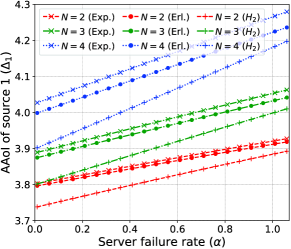
Figure 5: The AAoI of source s1subscript𝑠1s_{1} in terms of α𝛼\alpha for N={2,3,4}𝑁234N=\{2,3,4\} under various service time distributions. Here, 𝔼[S]=0.5𝔼𝑆0.5\operatorname{\mathbb{E}}[S]\!=\!0.5, 𝔼[R]=0.3𝔼𝑅0.3\operatorname{\mathbb{E}}[R]\!=\!0.3, α=0.1𝛼0.1\alpha\!=\!0.1, p=0.7𝑝0.7p\!=\!0.7, λ1=0.3subscript𝜆10.3\lambda_{1}=0.3, and λi(i1)=0.12subscript𝜆𝑖𝑖10.12\lambda_{i}(i\neq 1)\!=\!0.12.

Figure 5 plots the AAoI of s1subscript𝑠1s_{1} as a function of the server failure rate (α)𝛼(\alpha) for λ1=0.3subscript𝜆10.3\lambda_{1}\!=\!0.3. By comparing the service time distributions for various N𝑁N values, we note that the exponential distribution (Exp.), where p=1𝑝1p\!=\!1, yields the highest Δ1subscriptΔ1\Delta_{1}, which is then followed by the Erlang distribution. As the server experiences more frequent failures, the AAoI of s1subscript𝑠1s_{1} under all three distributions can be seen to converge. This is merely because most of the service time is spent repairing the server, leaving lesser time for the packets to be processed. It is also noteworthy that, irrespective of the service time distribution, QM exhibits system instability much earlier in time than BL when all sources generate packets at higher rates.

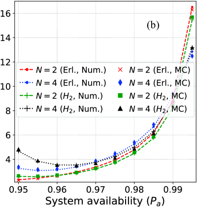
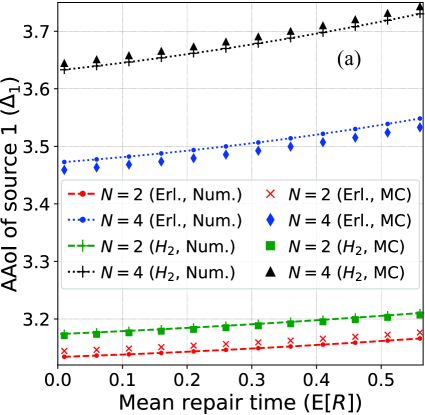
Finally, Figure 6 showcases the AAoI of s1subscript𝑠1s_{1} in terms of the mean repair time (𝔼[R])𝔼𝑅(\operatorname{\mathbb{E}}[R]) and the steady-state system availability (Pa)subscript𝑃𝑎(P_{a}). To corroborate the numerical results, we conduct Monte Carlo (MC) simulations where each data point is averaged over 100010001000 runs. In Figure 6a, we see that Δ1subscriptΔ1\Delta_{1} gradually increases with 𝔼[R]𝔼𝑅\operatorname{\mathbb{E}}[R], which is conforming to the system behavior depicted in Figure 5. As N𝑁N grows, the mean repair time also increases because the server fails more frequently thus, causing the AAoI of s1subscript𝑠1s_{1} to rise. As per (12), we see that Pasubscript𝑃𝑎P_{a} reaches its lowest value of 0.950.950.95 when λ1(=0.6)annotatedsubscript𝜆1absent0.6\lambda_{1}(=0.6) is the highest in Figure 6b. This implies that the server is more likely to process the increasing number of packets generated by s1subscript𝑠1s_{1}, thus resulting in lower Δ1subscriptΔ1\Delta_{1} values. However, gradual decrease in λ1subscript𝜆1\lambda_{1} causes Pasubscript𝑃𝑎P_{a} to rise. At Pa=0.995subscript𝑃𝑎0.995P_{a}\!=\!0.995, where λ1=0.06subscript𝜆10.06\lambda_{1}\!=\!0.06, packets generated by the other sources are primarily served due to their higher arrival rates (λi(i1)=0.12)subscript𝜆𝑖𝑖10.12(\lambda_{i}(i\!\neq\!1)\!=\!0.12). Such behavior explains the drastic increase of Δ1subscriptΔ1\Delta_{1} depicted in Figure 6b, despite the server availability being at its peak.

VI Conclusion

In this paper, we analyzed the average AoI of each source in a multi-source M/G/1 queueing model with active server breakdowns and general repair time. Using the supplementary variable technique, we first derived the pgf of AoI and the stationary distribution in a single-source unreliable M/G/1 queue. Then, the average AoI expression for the unreliable multi-source M/G/1 queue was derived in closed form. The analytical findings were validated for varying packet arrival and server failure rates under general service time distribution via simulation results. A possible avenue of future work is AoI analysis of correlated Poisson arrivals from multiple sources in unreliable queueing models.
Refer to caption

Refer to caption

Figure 6: The AAoI of source s1subscript𝑠1s_{1} in terms of (a) 𝔼[R]𝔼𝑅\operatorname{\mathbb{E}}[R] for λ1=0.3subscript𝜆10.3\lambda_{1}\!=\!0.3 and (b) Pasubscript𝑃𝑎P_{a} for λ1=[0.06,0.6]subscript𝜆10.060.6\lambda_{1}\!=\![0.06,0.6] and 𝔼[R]=0.3𝔼𝑅0.3\operatorname{\mathbb{E}}[R]=0.3. Here, N={2,4}𝑁24N\!=\!\{2,4\}, p=0.7𝑝0.7p\!=\!0.7, 𝔼[S]=0.5𝔼𝑆0.5\operatorname{\mathbb{E}}[S]=0.5, α=0.1𝛼0.1\alpha=0.1, and λi(i1)=0.12subscript𝜆𝑖𝑖10.12\lambda_{i}(i\neq 1)\!=\!0.12.

Appendix A Proof of Lemma 1

The first conditional expression in (15) can be written as:

𝔼[R1,ibX1,i|A1,ib]=𝔼[T1,i1X1,i|A1,ib]𝔼[X1,i2|A1,ib].𝔼conditionalsubscriptsuperscript𝑅𝑏1𝑖subscript𝑋1𝑖subscriptsuperscript𝐴𝑏1𝑖𝔼conditionalsubscript𝑇1𝑖1subscript𝑋1𝑖subscriptsuperscript𝐴𝑏1𝑖𝔼conditionalsubscriptsuperscript𝑋21𝑖subscriptsuperscript𝐴𝑏1𝑖\displaystyle\operatorname{\mathbb{E}}[R^{b}_{1,i}X_{1,i}|A^{b}_{1,i}]=\operatorname{\mathbb{E}}[T_{1,i-1}X_{1,i}|A^{b}_{1,i}]-\operatorname{\mathbb{E}}[X^{2}_{1,i}|A^{b}_{1,i}].\vspace{-0.2em} (24)

The first term of (24) reduces to:

𝔼[\displaystyle\operatorname{\mathbb{E}}[ T1,i1X1,i|A1,ib]=00xtfX1,i,T1,i1|A1,ib(x,t)dxdt\displaystyle T_{1,i-1}X_{1,i}|A^{b}_{1,i}]=\!\int_{0}^{\infty}\!\!\int_{0}^{\infty}\!x\,t\,f_{X_{1,i},T_{1,i-1}|A^{b}_{1,i\!}}(x,t)\,\text{d}x\,\text{d}t
=1p1,ib(𝔼[W]λ1+𝔼[S]λ1W(λ1)λ1W′′(λ1)),absent1subscriptsuperscript𝑝𝑏1𝑖𝔼𝑊subscript𝜆1𝔼𝑆subscript𝜆1superscript𝑊superscriptsubscript𝜆1subscript𝜆1superscript𝑊superscript′′subscript𝜆1\displaystyle=\dfrac{1}{p^{b}_{1,i}}\left(\dfrac{\operatorname{\mathbb{E}}[W]}{\lambda_{1}}+\dfrac{\operatorname{\mathbb{E}}[S]}{\lambda_{1}}-\dfrac{W^{*^{\prime}\!}(\lambda_{1})}{\lambda_{1}}-W^{*^{\prime\prime}\!}(\lambda_{1})\right),\vspace{-0.2em} (25)

where Wsuperscript𝑊superscriptW^{*^{\prime}\!} and W′′superscript𝑊superscript′′W^{*^{\prime\prime}\!} are, respectively, the first and second order derivatives of Wsuperscript𝑊W^{*} w.r.t. λ1subscript𝜆1\lambda_{1}. The second term of (24) reduces to:

𝔼[\displaystyle\operatorname{\mathbb{E}}[ X1,i2|A1,ib]=0x2fX1,i|A1,ib(x)dx\displaystyle X^{2}_{1,i}|A^{b}_{1,i}]=\!\int_{0}^{\infty}\!x^{2}\,f_{X_{1,i}|A^{b}_{1,i}}(x)\,\text{d}x
=1p1,ib(2λ12W′′(λ1)λ122W(λ12)λ12+2W(λ1)λ12).absent1subscriptsuperscript𝑝𝑏1𝑖2superscriptsubscript𝜆12superscript𝑊superscript′′subscript𝜆1superscriptsubscript𝜆122superscript𝑊superscriptsuperscriptsubscript𝜆12superscriptsubscript𝜆122superscript𝑊subscript𝜆1superscriptsubscript𝜆12\displaystyle=\dfrac{1}{p^{b}_{1,i\!}}\!\left(\!\dfrac{2}{\lambda_{1}^{2}}\!-\!\dfrac{W^{*^{\prime\prime}\!}(\lambda_{1})}{\lambda_{1}^{2}}-\dfrac{2W^{*^{\prime}\!}(\lambda_{1}^{2})}{\lambda_{1}^{2}}+\dfrac{2W^{*\!}(\lambda_{1})}{\lambda_{1}^{2}}\!\right).\vspace{-0.2em} (26)

Adding (25) and (26) gives (18), which completes the proof.

Appendix B Proof of Lemma 2

The second conditional expression in (15) can be written as:

𝔼[\displaystyle\operatorname{\mathbb{E}}[ G1,ibX1,i|A1,ib]\displaystyle G^{b}_{1,i}X_{1,i}|A^{b}_{1,i}]
=0x𝔼[iΩ2,ibS2,iA1,ib,X1,i=x]fX1,i|A1,ib(x)dx.absentsuperscriptsubscript0𝑥𝔼conditionalsubscriptsuperscript𝑖subscriptsuperscriptΩ𝑏2𝑖subscript𝑆2superscript𝑖subscriptsuperscript𝐴𝑏1𝑖subscript𝑋1𝑖𝑥subscript𝑓conditionalsubscript𝑋1𝑖subscriptsuperscript𝐴𝑏1𝑖𝑥d𝑥\displaystyle=\int_{0}^{\infty}\!\!x\operatorname{\mathbb{E}}\big{[}\!\!\!\sum_{i^{\prime}\in\Omega^{b}_{2,i}}\!\!\!S_{2,i^{\prime}\!}\!\mid\!A^{b}_{1,i},X_{1,i}\!=\!x]f_{\!X_{1\!,i}|A^{b}_{1,i\!\!}}(x)\,\text{d}x.\vspace{-0.6em} (27)

The set Ω2,ibsubscriptsuperscriptΩ𝑏2𝑖\Omega^{b}_{2,i} in (27) denotes the packets generated from s2subscript𝑠2s_{2} that must be served before those from s1subscript𝑠1s_{1} and is independent of the inter-arrival time of s1subscript𝑠1s_{1} packets (T1,i1)subscript𝑇1𝑖1(T_{1,i-1}). Thus, we get:

𝔼[G1,ibX1,i|A1,ib]=ρ2p1,ib0x2λ1eλ1x(1FT1,i1(x))dx,𝔼conditionalsubscriptsuperscript𝐺𝑏1𝑖subscript𝑋1𝑖subscriptsuperscript𝐴𝑏1𝑖subscript𝜌2subscriptsuperscript𝑝𝑏1𝑖superscriptsubscript0superscript𝑥2subscript𝜆1superscript𝑒subscript𝜆1𝑥1subscript𝐹subscript𝑇1𝑖1𝑥d𝑥\displaystyle\operatorname{\mathbb{E}}[G^{b}_{1\!,i}X_{1\!,i}|A^{b}_{1\!,i}]\!=\!\dfrac{\rho_{2}}{p^{b}_{1\!,i}\!}\int_{0}^{\infty}\!\!x^{2}\lambda_{1}e^{\!-\lambda_{1}x\!}\left(\!1\!-\!F_{T_{1\!,i\!-\!1\!}}(x)\right)\text{d}x,\vspace{-0.6em} (28)

which after some algebraic manipulations and rearrangements, results in (19). This completes the proof.

Appendix C Proof of Lemma 3

The third conditional expression in (15) can be reduced as:

𝔼𝔼\displaystyle\operatorname{\mathbb{E}} [(G1,il+R2,il)X1,i|A1,il]delimited-[]conditionalsubscriptsuperscript𝐺𝑙1𝑖subscriptsuperscript𝑅𝑙2𝑖subscript𝑋1𝑖subscriptsuperscript𝐴𝑙1𝑖\displaystyle\!\left[\left(G^{l}_{1\!,i}\!+\!R^{l}_{2,i}\right)X_{\!1\!,i}|A^{l}_{1\!,i}\right]
=ρ2p1,il0txtλ1eλ1xfT1,i1(t)dxdtabsentsubscript𝜌2subscriptsuperscript𝑝𝑙1𝑖superscriptsubscript0superscriptsubscript𝑡𝑥𝑡subscript𝜆1superscript𝑒subscript𝜆1𝑥subscript𝑓subscript𝑇1𝑖1𝑡d𝑥d𝑡\displaystyle\quad=\dfrac{\rho_{2}}{p^{l}_{1,i}}\!\int_{0}^{\infty}\!\!\int_{t}^{\infty}\!\!x\,t\,\lambda_{1}e^{-\lambda_{1}x}f_{T_{1,i-1\!}}(t)\,\text{d}x\,\text{d}t
=ρ2p1,il0(t2eλ1xfT1,i1(t)+tλ1eλ1xfT1,i1(t))dt,absentsubscript𝜌2subscriptsuperscript𝑝𝑙1𝑖superscriptsubscript0superscript𝑡2superscript𝑒subscript𝜆1𝑥subscript𝑓subscript𝑇1𝑖1𝑡𝑡subscript𝜆1superscript𝑒subscript𝜆1𝑥subscript𝑓subscript𝑇1𝑖1𝑡d𝑡\displaystyle\quad=\dfrac{\rho_{2}}{p^{l}_{1,i}}\!\int_{0}^{\infty}\!\!\left(\!t^{2}e^{\!-\lambda_{1}x}f_{T_{1,i-1\!}}(t)\!+\!\dfrac{t}{\lambda_{1}}e^{\!-\lambda_{1}x}f_{T_{1,i-1\!}}(t)\!\right)\text{d}t,\vspace{-0.7em} (29)

which after some algebraic manipulations and rearrangements, results in (20). This completes the proof.

References

  • [1] R. D. Yates, Y. Sun, D. R. Brown, S. K. Kaul, E. Modiano, and S. Ulukus, “Age of information: An introduction and survey,” IEEE J. Sel. Areas Commun., vol. 39, no. 5, pp. 1183–1210, May 2021.
  • [2] A. Baiocchi and I. Turcanu, “Age of information of one-hop broadcast communications in a CSMA network,” IEEE Commun. Lett., vol. 25, no. 1, pp. 294–298, Jan. 2021.
  • [3] M. Moradian and A. Dadlani, “Average age of information in two-way relay networks with service preemptions,” in Proc. IEEE Global Commun. Conf. (GLOBECOM), 2021, pp. 1–6.
  • [4] N. I. Miridakis, T. A. Tsiftsis, and G. Yang, “Non-linear age of information: An energy efficient receiver-centric approach,” IEEE Wireless Commun. Lett., vol. 11, no. 3, pp. 655–659, Mar. 2022.
  • [5] S. Kaul, R. Yates, and M. Gruteser, “Real-time status: How often should one update?” in Proc. IEEE Int. Conf. Comput. Commun. (INFOCOM), Mar. 2012, pp. 2731–2735.
  • [6] R. D. Yates and S. K. Kaul, “The age of information: Real-time status updating by multiple sources,” IEEE Trans. Inf. Theory, vol. 65, no. 3, pp. 1807–1827, Mar. 2019.
  • [7] E. Najm and E. Telatar, “Status updates in a multi-stream M/G/1/1 preemptive queue,” in Proc. IEEE Conf. Comp. Commun. Workshops (INFOCOM WKSHPS), Apr. 2018, pp. 124–129.
  • [8] M. Moltafet, M. Leinonen, and M. Codreanu, “On the age of information in multi-source queueing models,” IEEE Trans. Commun., vol. 68, no. 8, pp. 5003–5017, Aug. 2020.
  • [9] ——, “Moment generating function of the AoI in a two-source system with packet management,” IEEE Wireless Commun. Lett., vol. 10, no. 4, pp. 882–886, Apr. 2021.
  • [10] M. A. Abd-Elmagid and H. S. Dhillon, “Closed-form characterization of the MGF of AoI in energy harvesting status update systems,” IEEE Trans. Inf. Theory, vol. 68, no. 6, pp. 3896–3919, Jun. 2022.
  • [11] V. Tripathi, R. Talak, and E. H. Modiano, “Age of information for discrete time queues,” CoRR, vol. abs/1901.10463, 2019. [Online]. Available: http://arxiv.org/abs/1901.10463
  • [12] J. Xu, I.-H. Hou, and N. Gautam, “Age of information for single buffer systems with vacation server,” IEEE Trans. Netw. Sci. Eng., vol. 9, no. 3, pp. 1198–1214, May-Jun. 2022.
  • [13] L. Kleinrock, Queueing Systems Volume 1: Theory.   Wiley, 1975.