Approximate Bayesian Neural Operators: Uncertainty Quantification for Parametric PDEs

Abstract

Neural operators are a type of deep architecture that learns to solve (i.e. learns the nonlinear solution operator of) partial differential equations (PDEs). The current state of the art for these models does not provide explicit uncertainty quantification. This is arguably even more of a problem for this kind of tasks than elsewhere in machine learning, because the dynamical systems typically described by PDEs often exhibit subtle, multiscale structure that makes errors hard to spot by humans. In this work, we first provide a mathematically detailed Bayesian formulation of the “shallow” (linear) version of neural operators in the formalism of Gaussian processes. We then extend this analytic treatment to general deep neural operators using approximate methods from Bayesian deep learning. We extend previous results on neural operators by providing them with uncertainty quantification. As a result, our approach is able to identify cases, and provide structured uncertainty estimates, where the neural operator fails to predict well.

1 Introduction

Neural operators [Li et al., 2020b, 2021a, a, 2021b, Kovachki et al., 2021] are a deep learning architecture tailored to reconstruction problems related to partial differential equations. They approximate mappings between infinite-dimensional vector spaces of functions, such that – once trained – solutions of entire families of parametric partial differential equations (PDEs) can be represented by a single neural network. This process is subject to several sources of uncertainty, which can result in a potentially significant prediction error because of the nonlinear – and nonintuitive – interactions of different stages of the approximation. The goal of this paper is to develop methods for estimating this error at a practically acceptable computational cost. This kind of functionality is urgently needed in this domain: Due to the intricate and often not intuitive nature of the dynamical systems described by PDEs, it can be hard for the human eye to detect prediction errors, even when they are large.

In this paper, we develop an approximate Bayesian framework for neural operators – from a theoretical, and a computational point of view. We begin with a brief review of neural operators. Then, using linear, parametric PDEs as guiding examples, we show how their “shallow” (single-layer) base case allows an analytic Bayesian treatment in the formalism of Gaussian processes (Rasmussen and Williams [2006]). Even though PDEs are linear, the parameter-to-solution operators are not. Although this linear case is primarily of theoretical interest, it forms a core contribution of this paper that may make this model class more easily accessible to the Bayesian machine learning community. We then extend the theoretical analysis to the deep case. Here, analytic treatments are no longer possible, so we fall back on approximations developed for Bayesian deep learning. Specifically, we focus on Laplace approximations [MacKay, 1992] which are easy to add post-hoc even to pretrained networks, and add only moderate computational cost relative to deep training without uncertainty quantification [Daxberger et al., 2021]. We show in experiments that the resulting method can capture structure in predictive error both in the over- and under-sampled regime. In Section 2 we discuss some theoretical background and develop a probabilistic framework for neural operators. We discuss the related work in Section 3. In Section 4 we provide empirical results.

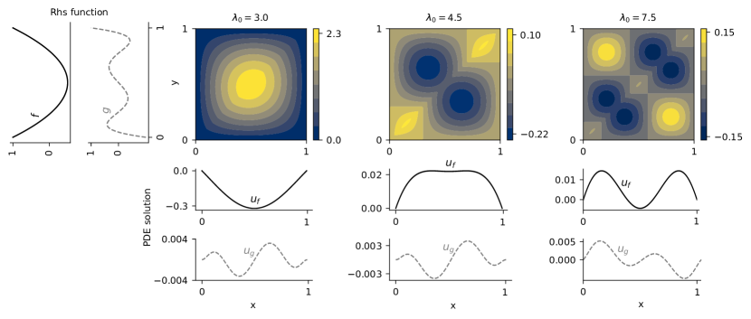
Figure 1: Green’s functions in Equation 6 for different values of $\lambda_{0}=\{3,4.5,7.5\}$. On the left, right-hand-side functions $f$, $g$ for the PDE in Equation 5 and respective solutions $u_{f}$, $u_{g}$ for the correspondent $\lambda_{0}$-value, computed through Equation 4.

2 METHOD

2.1 PDEs And Green’s Function

One of the main fields of applications of neural operators are partial differential equations (PDEs). In this work we consider the family of parametric PDEs

$$\begin{split}\big{(}\mathcal{L}_{\lambda}u\big{)}(x)&=f(x),\ \ \ x\in D\\ u(x)&=0,\ \ \ \ \ \ \ \ x\in\partial D\end{split}$$ (1)

for some sufficiently well-behaved, bounded domain $D\subset\mathbb{R}^{d}$ with boundary $\partial D$ (e.g. open, bounded $D$ with Lipschitz boundary $\partial D$), where $U\ni u\colon D\rightarrow\mathbb{R}$, $F\ni f\colon D\rightarrow\mathbb{R}$, $\lambda\in\Lambda$, with $U$, $F$ and $\Lambda$ appropriate function spaces. The precise nature of those function spaces is not important for the remainder of this work. The function $\lambda$ parametrises the differential operator $\mathcal{L}_{\lambda}$.

Equation 1 defines a solution operator

$$\mathcal{H}\colon\Lambda\times F\rightarrow U,\quad(\lambda,f)\mapsto u_{\lambda,f}$$ (2)

in the sense that $\mathcal{H}(\lambda,f)(x)=u_{\lambda,f}(x)$ solves the PDE for the given functions $\lambda$ and $f$. Even though the PDE is linear, $\mathcal{H}$ is (possibly highly) nonlinear. In particular, here we consider the case where $\lambda$ is fixed, so the solution operator can be written as

$$\mathcal{G}\colon f\mapsto u.$$ (3)

The operator $\mathcal{G}$, like $\mathcal{H}$, is a map between function spaces. The idea behind neural operators is to approximate the operator $\mathcal{G}$ (or $\mathcal{H}$) with a single neural network trained on function observations ${\{f_{i},u_{i}\}}_{i=1}^{N}$. Thus, instead of approximating the solution of the PDE for only a fixed $f$, neural operators directly infer the operator $\mathcal{G}$.

Numerically, the functions $f$ and $u$ are observed on a discretisation grid of the function domains. Considering the operator in Equation 3 is a key step to understand the learning process of neural operators. In fact, observe how $\mathcal{G}$ is the inverse of the operator $\mathcal{L}_{\lambda}$. The neural operator is therefore learning an operator, $\mathcal{G}$, through function observations ${\{f_{i},u_{i}\}}_{i=1}^{N}$ that derive from the action of its inverse. In other words, during training, the neural operator is implicitly learning to invert the differential operator $\mathcal{L}_{\lambda}$. In particular, in the case where the differential operator is linear and admits a Green’s function $G$, the solution of Equation 1 can be expressed through integration with the kernel $G$

$$u_{\lambda}(x)=\int_{D}G_{\lambda}(x,y)f(y)\,\text{d}y.$$ (4)

Hence, learning the operator $\mathcal{G}$ is here equivalent to learn the function $G$ which means that an operator-learning task can be reduced to that of function-reconstruction. The structure of neural operators in its one-layer case is inspired by the Green’s solution formula for linear PDEs in Equation 4. We will examine their architecture, in the more general case, in the next section.

In the general analysis of linear PDEs (we refer to e.g. Evans [2010] for background on PDEs), the Green’s function $G(x,y)$ represents the impulse response of the linear operator $\mathcal{L}_{\lambda}$, that is $\mathcal{L}_{\lambda}(G)(\cdot,y)=\delta(\cdot-y)$ for $y\in D$, where $\delta$ denotes the Dirac delta distribution. Note how $\mathcal{L}_{\lambda}$ is a linear operator, whereas the Green’s function is usually nonlinear in either arguments. To visualize the presented concepts, we consider the boundary value problem

$$\begin{split}\big{(}-\Delta-\lambda_{0}^{2}\operatorname{Id}\big{)}\ u(x)&=f(x),\ \ \ x\in[0,1],\\ u(0)=u(1)&=0,\end{split}$$ (5)

that admits a Green’s function in closed form,

$$G_{\lambda_{0}}(x,y):=\frac{A+B}{\lambda_{0}\sin(\lambda_{0})}$$ (6)

where we abbreviated

$$A :=H(y-x)\sin(\lambda_{0}x)\sin(\lambda_{0}(1-y))$$ (7)

$$B :=H(x-y)\sin(\lambda_{0}(1-x))\sin(\lambda_{0}y),$$ (8)

and $H$ denotes the Heaviside step function. Equation 5 relates to Equation 1 in the sense that the differential operator $\mathcal{L}_{\lambda_{0}}=(-\Delta-\lambda_{0}^{2}\operatorname{Id})$ is parametrised by $\lambda_{0}$. Green’s functions $G_{\lambda_{0}}$ for different values of $\lambda_{0}$, as well as the solutions computed through the solution formula in Equation 4, are depicted in Figure 1.

Figure 2: Neural operator architecture $\operatorname{NO}_{\Theta}$. Each layer $l$ computes a new function $\psi_{l}$, that contains the neural network $g_{\theta}$ in the integrand. Parameters of the layers are depicted on the respective arrows. The input function $f$ enters as an ”initialisation” only in the first layer, whereas the function $\lambda$ enters in $g_{\theta}$ at every $\psi_{l}$.

2.2 Neural Operator Essentials

Before formulating a Bayesian framework for neural operators, we recall their structure. A more thorough explanation of what follows can be found in the work by Li et al. [2020b, 2021a, a, 2021b], Kovachki et al. [2021].

A neural operator is a neural network architecture designed to approximate the general solution operator $\mathcal{H}$ in Equation 2. For particular cases, such as the operator $\mathcal{G}$ in Equation 3 where $\lambda$ is fixed, or for operators mapping $\lambda\mapsto u$ (where $f$ is fixed), an analogous construction is straight forward.

Let $g_{\theta}:D\times D\times\mathbb{R}\times\mathbb{R}\rightarrow\mathbb{R}$ be a neural network with parameters $\theta$. Define the neural operator $\operatorname{NO}_{\Theta}$ as a composition of $L\in\mathbb{N}$ layers

$$\operatorname{NO}_{\Theta}\colon\Lambda\times F \rightarrow U,$$

$$(\lambda,f) \mapsto(\psi_{L}\circ\psi_{L-1}\circ...\circ\psi_{1})(\lambda,f),$$ (9)

where each layer

$$\psi_{\ell}:\Phi\rightarrow\Phi,\quad\ell=\{1,\dots L\},$$ (10)

is defined as a composition of (i) integrating the output of the previous layer against $g_{\theta}$, and (ii) combining the integral with a linear component and an activation function $\sigma$,

$$\psi_{\ell}(g)(x)=\\ \sigma\bigg{(}W_{\ell}g(x)+\int_{D}g_{\theta}(x,y,\lambda(x),\lambda(y))g(y)\,\text{d}y\bigg{)}.$$ (11)

$\Phi$ is a vector space of functions mapping from $D$ to $\mathbb{R}$. The final layer of the neural operator maps into $U$, $\psi_{L}\colon\Phi\rightarrow U$. In practice, the integral cannot be computed in closed-form and a suitable quadrature formula needs to be employed (which turns the integral into a weighted sum of evaluations of the integrand; see e.g. [Davis and Rabinowitz, 2007]). The parameters $\Theta$ of $\operatorname{NO}_{\Theta}$ include the parameters $\theta$ of $g_{\theta}$ as well as the weights in each layer $W_{\ell}$, i.e. $\Theta=\theta\cup{\{W_{\ell}\}}_{\ell=1}^{L}$. Loosely speaking, one can think of this construction as a deep neural network ($\operatorname{NO}_{\Theta}$) that iteratively approximates the solution $u_{\lambda,f}$ (see Equation 2) and at every iteration (layer) employs another neural network ($g_{\theta}$). For a visualisation of $\operatorname{NO}_{\Theta}$ see Figure 2.

This architecture is inspired by the process of solving linear PDEs with Green’s functions: In the case where $L=1$, $\lambda\equiv\lambda_{0}^{2}$, $\sigma=\operatorname{Id}$, and $W_{1}=0$, and we consider the mapping $\mathcal{G}\colon f\mapsto u$, the neural operator approximating $\mathcal{G}$ becomes

$$\operatorname{NO}_{\Theta}(f)=\operatorname{NO}_{\theta}(f)=\int_{D}g_{\theta}(x,y)f(y)\,\text{d}y.$$ (12)

If $g_{\theta}$ is a sufficiently accurate approximation of the Green’s function $G_{\lambda_{0}}$ in Equation 6, Equation 12 is the solution formula of the PDE in Equation 5. In the next section we will provide a probabilistic formulation of the one layer architecture in Equation 12 that is based on the formalism of Gaussian processes.

Note how $\operatorname{NO}_{\Theta}$ approximates an operator. While, technically speaking, this means that its training and test set consist of functions, in the numerical computation, these functions need to be observed on some grid. Let $\{\lambda_{1},...,\lambda_{N}\}\times\{f_{1},...,f_{M}\}$ be a set of training inputs, each of which shall be observed on some mesh $\mathbb{X}:=\{x_{1},...,x_{K}\}$. In total, that makes $NK\times MK=NMK^{2}$ training inputs. Without loss of generality, and for the sake of simple notation, assume that the solution of the PDE and the respective inputs are observed on the same mesh $\mathbb{X}$. Thus, we observe $NM$ solutions $u_{11},...,u_{NM}$, i.e. $NMK$ training outputs – one set of evaluations at $\mathbb{X}$ for each solution $u_{nm}$ associated with $(\lambda_{n},f_{m})$, $n=1,...,N$, $m=1,...,M$. Each of these outputs is a function that maps from $D$ to $\mathbb{R}$, thus $u_{nm}(\mathbb{X})\in\mathbb{R}^{K}$. The relation between inputs and outputs is

$$u_{nm}=\mathcal{H}(\lambda_{n},f_{m}){\approx}\operatorname{NO}_{\Theta}(\lambda_{n},f_{m}).$$ (13)

While this equation is between functions, once discretised, it becomes an equation between vectors. To be able to optimise the parameters, we introduce the loss function

$$\mathcal{L}:\mathbb{R}^{K}\times\mathbb{R}^{K}\rightarrow[0,\infty).$$ (14)

The network parameters $\Theta$ are then computed by (approximately) solving the minimisation problem

$$\Theta^{*}=\arg\min_{\Theta}\sum_{n,m}\mathcal{L}(u_{nm}(\mathbb{X}),\operatorname{NO}_{\Theta}(\lambda_{n},f_{m})(\mathbb{X})),$$ (15)

where we used the above vectorised notation. This minimisation can be carried out with any of the optimisers popular in deep learning (see e.g. [Le et al., 2011]). Note that by approximating directly the solution operator $\mathcal{H}$, $\operatorname{NO}_{\Theta}$ simultaneously learns the entire family of PDEs parametrised by $f,\lambda$ without the need of re-training the network for a new $\lambda$ or $f$. Considering that these new inputs samples can be out of distribution cases, which are notoriously harder to predict [Hendrycks and Gimpel, 2017], it is even more important to introduce uncertainty quantification for these architectures.

2.3 Bayesian Neural Operators and Gaussian processes

Here we develop the Bayesian probabilistic framework for the neural operator. We start by observing that the special case of a one-layer network allows an analytic and in fact non-parametric Bayesian treatment through a Gaussian process model. This setting provides not just a useable algorithm, but also an important conceptual base-case that is not prominently discussed in previous works on neural operators (including non-Bayesian ones). In Section 2.4, this “shallow” treatment will be extended to the deep setting using a linearisation in form of the Laplace approximation, which again provides a Gaussian posterior distribution, albeit an approximate one.

Consider the solution operator $\mathcal{G}\colon f\mapsto u$ of the linear PDE in Equation 5. In this case $\mathcal{G}$ can be approximated with a one-layer neural operator, that in its single iteration computes the PDE solution as the integral

$$\operatorname{NO}_{\theta}=u_{f}(x)=\int_{D}g_{\theta}(x,y)f(y)\,\text{d}y.$$ (16)

As observed in Section 2.1, this “shallow” form of the neural operator is based on Green’s solution formulas for linear PDEs. Since the considered linear PDE admits an analytic Green’s function $G$ (see Equation 6), and since the only parameters of $\operatorname{NO}_{\Theta}$ are the ones of the neural network $g_{\theta}$, i.e. $\Theta=\theta$, learning the operator $\mathcal{G}$ is here equivalent to learning the function $G$. Therefore, for this setting, one can reformulate the task of inferring the solution operator $\mathcal{G}\colon f\mapsto u$ (which maps between infinite-dimensional vector spaces of functions) as the inference problem of learning the function $G\colon\mathbb{R}^{2}\rightarrow\mathbb{R}$.

In contrast to conventional GP regression, instead of direct observations of $G$, we only have access to $G$ through the integrals $u_{n}=\int_{D}G(x,y)f_{n}(y)\,\text{d}y$ for every data point $f_{n}$, $n=1,\dots,N$. We define the integral operator $\mathcal{A}_{f}=\mathcal{A}$ acting on $G$ as $\mathcal{A}G=\int_{D}G(\cdot,y)f(y)\,\text{d}y=u(\cdot)$. Since $\mathcal{A}$ is a linear operator, a Gaussian likelihood involving these observations (including the limit case of noise-free observations) remains conjugate to a GP prior and a Gaussian posterior can be computed in closed-form [Tanskanen et al., 2020, Longi et al., 2020].

Assume a Gaussian prior $G\sim\mathcal{GP}(\mu,k_{\theta})$ with mean function $\mu\colon\mathbb{R}^{2}\rightarrow\mathbb{R}$ and a parametrised kernel function $k_{\theta}\colon\mathbb{R}^{2}\times\mathbb{R}^{2}\rightarrow\mathbb{R}$. Assuming $u\mid G\sim\mathcal{N}(\mathcal{A}G,{\sigma^{2}})$, the posterior distribution over $G$ is a Gaussian process with mean and covariance

$$\begin{split}&\mathbb{E}[G]=\mu+\mathcal{A}^{\ast}k_{\theta}{(\mathcal{A}\mathcal{A}^{\ast}k_{\theta}+\sigma^{2})}^{-1}(u-\mathcal{A}\mu)\\ &\text{Cov}(G)=k_{\theta}-\mathcal{A}^{\ast}k_{\theta}{(\mathcal{A}\mathcal{A}^{\ast}k_{\theta}+\sigma^{2})}^{-1}\mathcal{A}k_{\theta}.\end{split}$$ (17)

where $\mathcal{A}^{\ast}$ is the adjoint of $\mathcal{A}$. With the posterior distribution over $G$ at hand we can compute uncertainty estimates on the prediction, draw posterior samples, and exploit all the other properties of GP regression. Moreover, the versatility of GPs allows to include prior information about $G$ in the kernel $k_{\theta}$. For example, the fact that Green’s functions are symmetric, i.e. $G(x,y)=G(y,x)$, can be encoded in $k_{\theta}$ (Duvenaud [2014]). Since the solution $u$ is a linear function of $G$, the Gaussian posterior over $G$ induces a GP over the solution $u$. That is, we obtain a probabilistic estimate over the PDE solution. Moreover, since we learned the solution operator $\mathcal{G}\colon f\mapsto u$, we directly obtain an estimate of all the PDE solutions for new right hand side functions $f^{\ast}$. In Section 4.1 we use this GP regression framework to learn the solution operator of Equation 5.

2.4 From GP To NN: Last-Layer Laplace Approximation On Neural Operators

While we can directly use GP regression to obtain uncertainty estimates on PDE solutions for the one-layer neural operator, this approach cannot be directly applied to deep neural operators, which contain non-linearities. However, we can use approximate inference techniques from Bayesian deep learning to obtain an approximation to the posterior distribution over the weights $p(\Theta\!\mid\!\mathcal{D})$ with $\mathcal{D}=\{\lambda_{n},f_{m},u_{nm}\}$, for $n=1,\dots,N$ and $m=1,\dots,M$. Since the computation of the true posterior is intractable, it is common to use a Gaussian approximation [MacKay, 1992, Blundell et al., 2015]. To make predictions with the approximate posterior $q(\Theta),$ we need the predictive distribution

$$\begin{split}p(u_{\ast}&\mid\operatorname{NO}_{\Theta}(\lambda_{\ast},f_{\ast}),\mathcal{D})\approx\\ &\int p(u_{\ast}\mid\operatorname{NO}_{\Theta}(\lambda_{\ast},f_{\ast}))q(\Theta)\,\text{d}\Theta\end{split}$$ (18)

for test functions $(\lambda_{\ast},f_{\ast})$. In general, computing this predictive distribution requires further approximation, such as the local linearisation of the neural network [Immer et al., 2020] which results in a Gaussian predictive distribution for a Gaussian likelihood. Alternatively, we can use a Laplace approximation, a relatively simple and early form of Bayesian deep learning [MacKay, 1992], on only the last layer of the network. This allows us to apply Laplace approximations to the intricate architecture of neural operators for efficient uncertainty quantification.

The Laplace approximation for neural networks requires a maximum a-posteriori (MAP) estimate which is obtained by minimizing the loss $\mathcal{L}(\mathcal{D};\Theta)$

$$\begin{split}\Theta_{\text{MAP}}&=\arg\min_{\Theta}\mathcal{L}(\mathcal{D};\Theta)\\ &=\arg\min_{\Theta}\big{(}r(\Theta)+\sum_{n,m}\ell(\lambda_{n},f_{m},u_{nm},\Theta)\big{)}.\end{split}$$ (19)

The empirical risk $\ell(\lambda_{n},f_{m},u_{nm},\Theta)$ corresponds to the negative log likelihood $-\log p(u_{nm}\mid\operatorname{NO}_{\Theta}(\lambda_{n},f_{m}))$ and the regularizer $r(\Theta)$ to the negative log prior distribution $-\log p(\Theta).$ The general idea of the Laplace approximation is to construct a local Gaussian approximation to the posterior $p(\Theta\mid\mathcal{D})$ by using a second order expansion of the loss $\mathcal{L}(\mathcal{D};\Theta)$ around $\Theta_{\text{MAP}}$

$$\begin{split}&\mathcal{L}(\mathcal{D};\Theta)\approx\mathcal{L}(\mathcal{D};\Theta_{\text{MAP}})\\ &+\frac{1}{2}{(\Theta-\Theta_{\text{MAP}})}^{\text{T}}\big{(}{\nabla_{\Theta}^{2}\mathcal{L}(\mathcal{D};\Theta)|}_{\Theta_{\text{MAP}}}\big{)}(\Theta-\Theta_{\text{MAP}}),\end{split}$$ (20)

where the first order term disappears at $\Theta_{\text{MAP}}$. Then the posterior approximation $q(\Theta)$ can be identified as a Gaussian centered at $\Theta_{\text{MAP}}$, with a covariance corresponding to the local curvature:

$$q(\Theta):=\mathcal{N}(\Theta\mid\Theta_{\text{MAP}},{({\nabla_{\Theta}^{2}\mathcal{L}(\mathcal{D};\Theta)|}_{\Theta_{\text{MAP}}})}^{-1}).$$ (21)

That is, the covariance is given by the inverse Hessian of the regularized training loss (which is interpreted as an unnormalized negative log posterior) at the trained weights $\Theta_{\text{MAP}}$.

A key practical advantage of this approach is that, since standard training of neural networks already identifies the local optimum $\Theta_{\text{MAP}}$, the only additional cost is to compute the Hessian $\nabla_{\Theta}^{2}\mathcal{L}(\mathcal{D};\Theta)$ at that point, once. This also means the approximation can be computed post-hoc, for pre-trained networks, which implies that uncertainty quantification in the form of a Laplace approximation comes only at a very small computational overhead while also preserving the predictive power of the maximum a posteriori estimate.

As mentioned before, we can use the decomposition of the neural operator into a fixed feature map corresponding to the first $L-1$ layers and a last linear layer [Snoek et al., 2015]. This is particularly convenient in the case of the architecture considered by Li et al. [2020b], since the last layer is indeed linear. Due to the linearity in the weights of the last layer, the distribution over the function outputs will also be Gaussian. Hence, for a Gaussian likelihood the predictive distribution in Equation 18 can be computed in closed form by using the approximate posterior $q(\Theta).$ Note that this predictive distribution is equivalent to the one of a GP regression problem [Khan et al., 2019]. This directly connects the GP approach for the shallow to the deep case, although we are now not approximating the posterior over the parameters of the Green function, but over the weights of the last layer.

Kristiadi et al. [2020], Daxberger et al. [2021] recently showed that this approach achieves competitive performance on many common uncertainty quantification benchmarks compared to more recent alternatives – despite the low computational overhead. Last-layer Laplace approximations may seem like a simplistic approach to quantifying uncertainty of intricate architectures such as as neural operators. In Section 4, we show empirically that this is not the case.

3 RELATED WORK

The interplay of (parametric) partial differential equation models (see Cohen and DeVore [2015] for a review) and deep learning has rapidly gained momentum in recent years. Broadly speaking, there are two approaches: learning the solution of a given PDE on the one hand, and learning the parameter-to-solution operator of a family of parametric PDEs on the other hand.

Conventional numerical PDE solvers (e.g. [Ames, 2014]) and physics-informed neural networks [Raissi et al., 2019, Sirignano and Spiliopoulos, 2018, Zhu et al., 2019] fall into the first category. In physics-informed neural networks, the PDE solution is modelled as a neural network. The differential equation is then translated into an appropriate loss function, and an approximate PDE solution emerges from automatic differentiation and numerical optimisation. While the physics-informed neural network formulation extends naturally to PDE inverse problems [Raissi et al., 2019, Zhu et al., 2019], it brings with it some practical issues like hyperparameter-sensitivity and complicated loss landscapes [Wang et al., 2021, Sun et al., 2020]. Physics-informed neural networks also need to be retrained once the parametrisation of the PDE ($\lambda$ of $f$) changes.

As described in Section 2.2, neural operators do not face this issue because they learn the parameter-to-solution operator of a family of parametric PDEs (recall Equation 2). They have been conceptualised by Lu et al. [2021], brought to the limelight by Bhattacharya et al. [2021], Nelsen and Stuart [2021], Li et al. [2020b, a, 2021a, 2021b], Patel et al. [2021], Duvall et al. [2021], Kovachki et al. [2021], and further extended by Guibas et al. [2022], Gupta et al. [2021], Rahman et al. [2022b], Fanaskov and Oseledets [2022], Rahman et al. [2022a]. They are equipped with uncertainty quantification in the present work. The effect of uncertainty quantification will be investigated in the experiments below, and extending the proposed methodology will be an important direction for future development of neural operators because the solution operators are highly nonlinear, and its recovery strongly depends on the training data. For sophisticated PDE models, training data is expensive to assemble because each training point relies on the numerical solution of a PDE. In those low-data regimes, uncertainty quantification equips a practitioner with the information of whether the recovery can be trusted or not.

A principled approach to uncertainty quantification is generally provided by Bayesian deep learning. Besides the Laplace approximation, which has been discussed in Section 2.4, there are many more approximate Bayesian methods for inferring the neural networks’ weights. These include variational inference [Graves, 2011, Blundell et al., 2015, Khan et al., 2018, Zhang et al., 2018], Markov Chain Monte Carlo [Neal, 1996, Welling and Teh, 2011, Zhang et al., 2020], and heuristic methods [Gal and Ghahramani, 2016, Maddox et al., 2019]. Typically, they employ a Gaussian posterior approximation. One crucial advantage of the Laplace approximation over many of these methods is that it can be applied post-hoc, i.e. it is not only cheap but also preserves the estimate returned by the preceding non-Bayesian computation, whereas other methods require retraining the network, which is expensive and might lead to worse predictive performance, since the optimization process is changed and the standard deep learning techniques and hyperparameter settings might not work anymore, which makes more tuning necessary; this is an additional cost factor besides the training itself.

4 Experiments

In this section we exploit the theoretical analysis developed in Section 2 to construct Bayesian neural operators delivering uncertainty estimates. We use the analytic GP framework of Section 2.3 to build a non-parametric Bayesian neural operator in the "shallow" case, then extend our method to the deep case. We reproduce the experiments on neural operators as carried out by Li et al. [2020b] to show that we can effectively detect wrong predictions.

4.1 Uncertainty Quantification in the Shallow Case with GP regression

Consider the boundary value problem in Equation 5 for a fixed $\lambda_{0}\in\mathbb{R}$. As discussed in Section 2.3, since the PDE is linear and admits the Green’s function $G\colon\mathbb{R}^{2}\rightarrow\mathbb{R}$ in Equation 6, inferring the solution operator $\mathcal{G}\colon f\mapsto u$ is equivalent to learning the function $G$ given integral observations ${\{f_{i},u_{i}=\int_{D}G(\cdot,y)f_{i}(y)\,\text{d}y\}}_{i=1}^{N}$. Note that every observation point is a function, numerically observed on a grid $\mathbb{X}=\{x_{1},\dots x_{K}\}$. As training points $\{f_{i}\}_{i=1}^{N}$ (right hand functions of the PDE in Equation 5) we use the first $N$ Legendre polynomials shifted on the interval $[0,1]$ and observed on an evenly spaced grid $\mathbb{X}=\{x_{1}=0,\dots x_{9}=1\}$. We assume a Gaussian prior $G\sim\mathcal{GP}(\mu,k)$ with a zero mean function $\mu$ and a kernel function $k\colon\mathbb{R}^{2}\times\mathbb{R}^{2}\rightarrow\mathbb{R}$ that factorizes into the product $k((x_{0},x_{1}),(y_{0},y_{1}))=k_{1}(x_{0},y_{0})k_{2}(x_{1},y_{1})$ where $k_{1}$ and $k_{2}$ are Matérn kernels with parameter $\nu=2.5$. To compute the integral operator $\mathcal{A}$ in Equation 17 we use numerical integration.

The posterior distribution over $G$ inferred with Equation 17 is shown in Figure 3. The figure shows the posterior distribution for $G$ after $N=3$ and $N=8$ function observations. Samples from the posterior are used to visualize the posterior variance; the very diverse samples after $N=3$ observations derive from a high variance, reflecting the fact that the approximation is imprecise. Instead, for $N=8$ the distribution exhibits low variance and an accurate estimate. Since by learning $G$ we learned the inverse of the differential operator in Equation 5, we can use the posterior distribution over $G$ to get an approximation, as well as an error estimate, of the solution for a new PDE with right hand side function $f^{\ast}$.

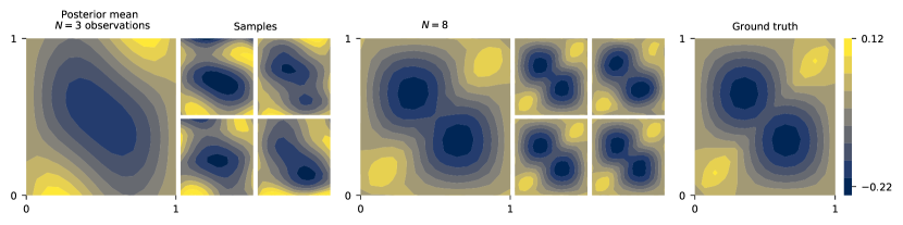
Figure 3: Posterior distribution on $G_{\lambda_{0}}$ for $\lambda_{0}=4.5$ (and ground truth) after $N=3,8$ observations $\{f_{i}\}_{i=1}^{N}$ with $f_{i}$ shifted Legendre polynomials. The samples show the approximation’s variance, which decreases when $N$ increases.

4.2 Uncertainty Quantification in the Deep Case

The examples considered in this section aim to emphasize the importance of uncertainty quantification for the complex architectures that are neural operators. We show that Bayesian neural operators are able not only to precisely detect areas of imprecise solution estimates, but in low sampling regimes they help preventing significant mistakes in the prediction. The fact that such mistakes can occur already in linear PDEs, which we consider in this section, further motivates the need for uncertainty estimates in the nonlinear case.

To recreate the results in Li et al. [2020b] we use their original code. As discussed in Section 2.4, our Bayesian framework computes Gaussian approximations of the posterior $p(\Theta\mid D)$ through Laplace approximations. For an efficient implementation of the last-layer Laplace approximation, we use the software library introduced by Daxberger et al. [2021]. We use a last-layer Laplace approximation with a full generalized Gauss-Newton approximation [Schraudolph, 2002] of the Hessian. There are two scalar hyperparameters, the prior precision and the observation noise. Both are tuned post hoc via optimizing the log marginal likelihood [Immer et al., 2021, Daxberger et al., 2021].

In their work, Li et al. [2020b] considered the second order elliptic PDE

$$\begin{split}-\nabla\cdot(\lambda(x)\nabla u(x))&=f(x),\quad x\in D\\ u(x)&=0\ \ \qquad x\in\partial D\end{split}$$ (22)

where $D=[0,1]^{2}$ is the unit square and $f\equiv 1$. The PDE in Equation 22 represents the steady state of a two dimensional Darcy flow and arises in several physical applications. The nonlinear solution operator

$$\mathcal{F}\colon\Lambda\rightarrow U,\quad\lambda\mapsto u$$ (23)

is approximated with a type of neural operator architecture based on graph neural network structures (Kipf and Welling [2017]). In particular, for the computation of the integral in Equation 11, the domain $D$ is discretised into a graph-structured data on which the message passing algorithm of Gilmer et al. [2017] is applied.

In Section 4.3 we examine the case where only few data are available. In Section 4.4 a high data regime is considered.

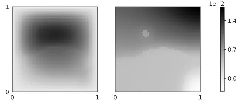
(a) The ground truth (left) and the approximation (right).

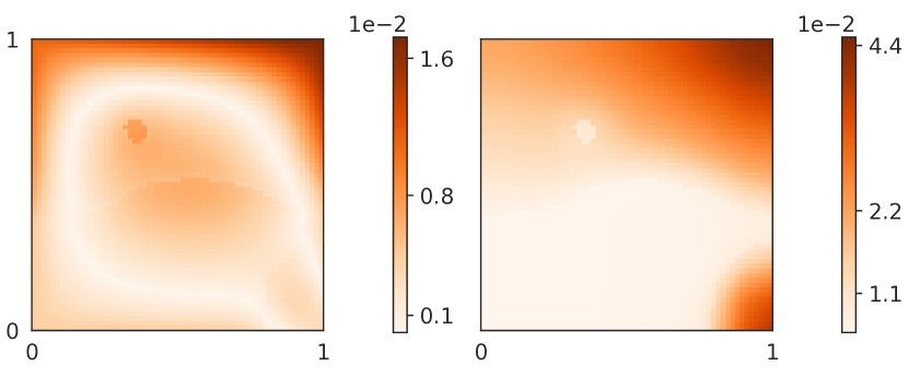
(b) The error (left) and the standard deviation (right).

Figure 4: The Bayesian neural operator on the 2d Darcy flow problem in the low-data regime. The approximation is relatively bad and the predictive standard deviation highlights the areas of high error.

4.3 Low-data Regime

At first, we consider the case where only few observation points on the unit square $D=[0,1]^{2}$ are available. Sparse observations are a common scenario for multi-scale dynamics described by PDEs, where data is usually not easily affordable. Due to the limited amount of data, approximated solutions can be very inaccurate. It is therefore fundamental to associate uncertainty to the outcome of the prediction.

In particular, since the problem is relatively simple, we consider an extreme setting where we train on only two training functions and subsample only two points from a $16\times 16$ grid for each. Figure 4 shows on a $61\times 61$ grid that in this setting the neural operator fails to predict the solution well. As a consequence, the Bayesian neural operator yields low confidence (high predictive standard deviation) in the prediction, particularly in the areas of higher error. For readability, the plots use different color scales. This is due to the slight underconfidence of the Laplace approximation (in the scalar global parameter, not the local structure). Having measures such as the predictive standard deviation to determine whether the prediction should be trusted is of big practical benefit for many applications.

4.4 High-data Regime

The previous section considered a heavily under-sampled problem. In this simple uni-variate toy problem, this meant using a very small number of training data. Nevertheless, the under-sampled regime is arguably the norm in practical problems with a more realistic, higher number of dimensions, where one can not hope to tile the domain with pre-computed PDE solutions. In this section, for completeness, we consider the other, over-sampled end of the spectrum and find that good and structured uncertainty quantification is nevertheless useful here.

Figure 5 shows results on a dense $61\times 61$ grid, analogous to the previous one, trained on 100 densely evaluated $16\times 16$ grid solutions. Note, that the model generalizes well from the smaller $16\times 16$ grid used during training to the larger $61\times 61$ grid for testing, as previously shown by Li et al. [2020b]. Although the prediction error is generally of good quality (i.e. relative prediction errors are mostly below 10%), the trained network exhibits an artifact in one, sharply delineated region of the training domain. This is not a bug, but a common problem with the ReLU features in this architecture, which create piecewise linear predictive regions [Hein et al., 2019].

As the figure shows, the Laplace approximation is in fact able to identify and delineate this region well, and produce an effective, well-calibrated warning about its presence. It is important to note that this kind of functionality is only possible with the structured uncertainty produced by a Bayesian technique like the Laplace approximation – i.e. by an approximate posterior measure, rather than a global worst-case error bound.

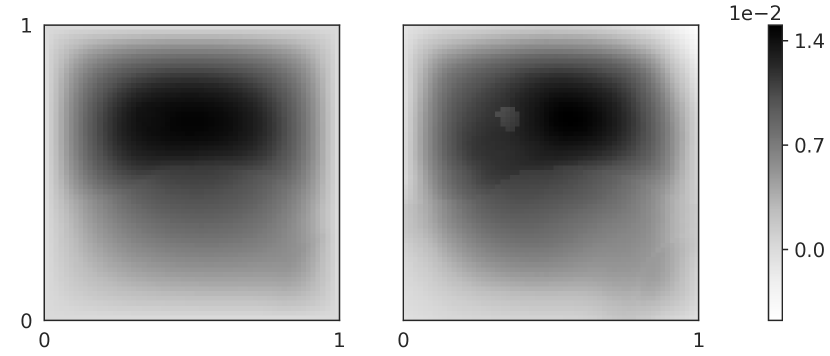
(a) The ground truth (left) and the approximation (right).

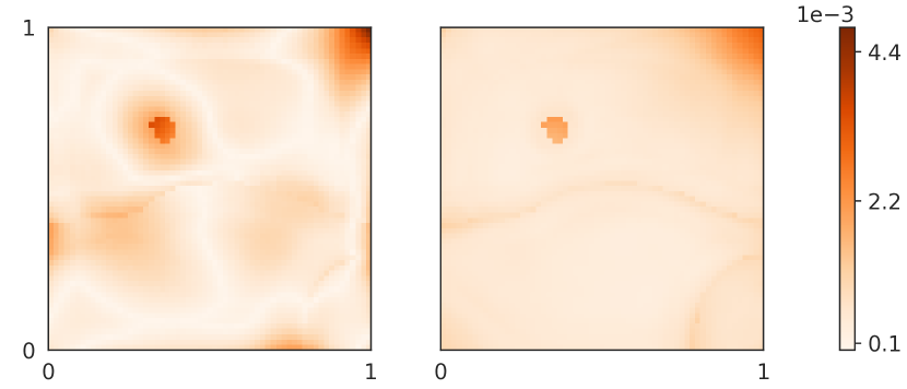
(b) The error (left) and the standard deviation (right).

Figure 5: The Bayesian neural operator on the 2d Darcy flow problem in the high-data regime. The approximation is close to the ground truth. The regions of relatively high error, as well as their magnitude, are captured by the predictive standard deviation.

5 CONCLUSIONS

We provided a theoretical Bayesian framework for neural operators. While these recently introduced architectures have shown to have a competitive performance with other numerical methods and to beat the state-of-the-art neural networks approaches on large grids, they did not previously come with explicit uncertainty quantification. We developed an explicit analytic Bayesian treatment for the linear base-case, and illustrated how we can learn (the distribution over) solution operators through non-parametric GP regression. We provided an effective and efficient approximate Bayesian treatment for the full, deep case through the use of Laplace approximations. In experiments, our approach is able to quantify predictive uncertainty both in the sparsely and densely sampled regime. In the former, it produces structured uncertainty across the predictive domain. In the latter, it is able to precisely detect and delineate regions where the predictive estimate fails to approximate the true solution well. The code used to produce the results herein will be released with the final version of this paper.

If deep learning approaches to the simulation of dynamical systems are to fulfill their potential and be applied to serious, large-scale partial differential equations (including safety-critical and scientific applications), then uncertainty quantification as presented here has a crucial role to play in the prevention of accidental and potentially dangerous prediction errors.

References

- Ames [2014] William F Ames. Numerical Methods for Partial Differential Equations. Academic Press, 2014.
- Bhattacharya et al. [2021] Kaushik Bhattacharya, Bamdad Hosseini, Nikola B Kovachki, and Andrew M Stuart. Model reduction and neural networks for parametric PDEs. The SMAI journal of computational mathematics, 7:121–157, 2021.
- Blundell et al. [2015] Charles Blundell, Julien Cornebise, Koray Kavukcuoglu, and Daan Wierstra. Weight uncertainty in neural network. In ICML, 2015.
- Cohen and DeVore [2015] Albert Cohen and Ronald DeVore. Approximation of high-dimensional parametric PDEs. Acta Numerica, 24:1–159, 2015.
- Davis and Rabinowitz [2007] Philip J Davis and Philip Rabinowitz. Methods of Numerical Integration. Courier Corporation, 2007.
- Daxberger et al. [2021] Erik Daxberger, Agustinus Kristiadi, Alexander Immer, Runa Eschenhagen, Matthias Bauer, and Philipp Hennig. Laplace redux – effortless Bayesian deep learning. In NeurIPS, 2021.
- Duvall et al. [2021] James Duvall, Karthik Duraisamy, and Shaowu Pan. Non-linear independent dual system (nids) for discretization-independent surrogate modeling over complex geometries. arXiv:2109.07018, 2021.
- Duvenaud [2014] David Duvenaud. Automatic model construction with Gaussian processes. PhD thesis, University of Cambridge, 2014.
- Evans [2010] Lawrence C. Evans. Partial Differential Equations. American Mathematical Society, 2010.
- Fanaskov and Oseledets [2022] Vladimir Fanaskov and Ivan Oseledets. Spectral neural operators. arXiv:2205.10573, 2022.
- Gal and Ghahramani [2016] Yarin Gal and Zoubin Ghahramani. Dropout as a Bayesian approximation: Representing model uncertainty in deep learning. In ICML, 2016.
- Gilmer et al. [2017] Justin Gilmer, Samuel S. Schoenholz, Patrick F. Riley, Oriol Vinyals, and George E. Dahl. Neural message passing for quantum chemistry. In ICML, 2017.
- Graves [2011] Alex Graves. Practical variational inference for neural networks. In NeurIPS, 2011.
- Guibas et al. [2022] John Guibas, Morteza Mardani, Zongyi Li, Andrew Tao, Anima Anandkumar, and Bryan Catanzaro. Adaptive Fourier neural operators: Efficient token mixers for transformers. In ICLR, 2022.
- Gupta et al. [2021] Gaurav Gupta, Xiongye Xiao, and Paul Bogdan. Multiwavelet-based operator learning for differential equations. In NeurIPS, 2021.
- Hein et al. [2019] Matthias Hein, Maksym Andriushchenko, and Julian Bitterwolf. Why ReLU networks yield high-confidence predictions far away from the training data and how to mitigate the problem. In CVPR, 2019.
- Hendrycks and Gimpel [2017] Dan Hendrycks and Kevin Gimpel. A baseline for detecting misclassified and out-of-distribution examples in neural networks. In ICLR, 2017.
- Immer et al. [2020] Alexander Immer, Maciej Korzepa, and Matthias Bauer. Improving predictions of Bayesian neural networks via local linearization. In AISTATS, 2020.
- Immer et al. [2021] Alexander Immer, Matthias Bauer, Vincent Fortuin, Gunnar Rätsch, and Mohammad Emtiyaz Khan. Scalable marginal likelihood estimation for model selection in deep learning. In ICML, 2021.
- Khan et al. [2018] Mohammad Emtiyaz Khan, Didrik Nielsen, Voot Tangkaratt, Wu Lin, Yarin Gal, and Akash Srivastava. Fast and scalable Bayesian deep learning by weight-perturbation in adam. In ICML, 2018.
- Khan et al. [2019] Mohammad Emtiyaz Khan, Alexander Immer, Ehsan Abedi, and Maciej Korzepa. Approximate inference turns deep networks into Gaussian processes. In NeurIPS, 2019.
- Kipf and Welling [2017] Thomas N. Kipf and Max Welling. Semi-supervised classification with graph convolutional networks. In ICLR, 2017.
- Kovachki et al. [2021] Nikola Kovachki, Zongyi Li, Burigede Liu, Kamyar Azizzadenesheli, Kaushik Bhattacharya, Andrew Stuart, and Anima Anandkumar. Neural operator: Learning maps between function spaces. arXiv:2108.08481, 2021.
- Kristiadi et al. [2020] Agustinus Kristiadi, Matthias Hein, and Philipp Hennig. Being Bayesian, even just a bit, fixes overconfidence in relu networks. In ICML, 2020.
- Le et al. [2011] Quoc V Le, Jiquan Ngiam, Adam Coates, Abhik Lahiri, Bobby Prochnow, and Andrew Y Ng. On optimization methods for deep learning. In ICML, 2011.
- Li et al. [2020a] Zongyi Li, Nikola Kovachki, Kamyar Azizzadenesheli, Burigede Liu, Kaushik Bhattacharya, Andrew Stuart, and Anima Anandkumar. Multipole graph neural operator for parametric partial differential equations. In NeurIPS, 2020a.
- Li et al. [2020b] Zongyi Li, Nikola Kovachki, Kamyar Azizzadenesheli, Burigede Liu, Kaushik Bhattacharya, Andrew Stuart, and Anima Anandkumar. Neural operator: Graph kernel network for partial differential equations. In ICLR 2020 Workshop on Integration of Deep Neural Models and Differential Equations, 2020b.
- Li et al. [2021a] Zongyi Li, Nikola Kovachki, Kamyar Azizzadenesheli, Burigede Liu, Kaushik Bhattacharya, Andrew Stuart, and Anima Anandkumar. Fourier neural operator for parametric partial differential equations. In ICLR, 2021a.
- Li et al. [2021b] Zongyi Li, Nikola Kovachki, Kamyar Azizzadenesheli, Burigede Liu, Kaushik Bhattacharya, Andrew Stuart, and Anima Anandkumar. Markov neural operators for learning chaotic systems. arXiv:2106.06898, 2021b.
- Longi et al. [2020] Krista Longi, Chang Rajani, Tom Sillanpää, Joni Mäkinen, Timo Rauhala, Ari Salmi, Edward Hæggström, and Arto Klami. Sensor placement for spatial Gaussian processes with integral observations. In UAI, pages 1009–1018. PMLR, 2020.
- Lu et al. [2021] Lu Lu, Pengzhan Jin, Guofei Pang, Zhongqiang Zhang, and George Em Karniadakis. Learning nonlinear operators via DeepONet based on the universal approximation theorem of operators. Nature Machine Intelligence, 3(3):218–229, 2021.
- MacKay [1992] David JC MacKay. The evidence framework applied to classification networks. Neural computation, 4(5):720–736, 1992.
- Maddox et al. [2019] Wesley Maddox, T. Garipov, Pavel Izmailov, Dmitry P. Vetrov, and Andrew Gordon Wilson. A simple baseline for Bayesian uncertainty in deep learning. In NeurIPS, 2019.
- Neal [1996] Radford M. Neal. Bayesian Learning for Neural Networks. Springer-Verlag, Berlin, Heidelberg, 1996. ISBN 0387947248.
- Nelsen and Stuart [2021] Nicholas H Nelsen and Andrew M Stuart. The random feature model for input-output maps between Banach spaces. SIAM Journal on Scientific Computing, 43(5):A3212–A3243, 2021.
- Patel et al. [2021] Ravi G Patel, Nathaniel A Trask, Mitchell A Wood, and Eric C Cyr. A physics-informed operator regression framework for extracting data-driven continuum models. Computer Methods in Applied Mechanics and Engineering, 373:113500, 2021.
- Rahman et al. [2022a] Md Ashiqur Rahman, Manuel A Florez, Anima Anandkumar, Zachary E. Ross, and Kamyar Azizzadenesheli. Generative adversarial neural operators. arXiv:2205.03017, 2022a.
- Rahman et al. [2022b] Md Ashiqur Rahman, Zachary E Ross, and Kamyar Azizzadenesheli. U-no: U-shaped neural operators. arXiv:2204.11127, 2022b.
- Raissi et al. [2019] Maziar Raissi, Paris Perdikaris, and George E Karniadakis. Physics-informed neural networks: A deep learning framework for solving forward and inverse problems involving nonlinear partial differential equations. Journal of Computational Physics, 378:686–707, 2019.
- Rasmussen and Williams [2006] CE. Rasmussen and CKI. Williams. Gaussian Processes for Machine Learning. Adaptive Computation and Machine Learning. MIT Press, January 2006.
- Schraudolph [2002] Nicol N. Schraudolph. Fast curvature matrix-vector products for second-order gradient descent. Neural Computation, 14(7):1723–1738, 2002.
- Sirignano and Spiliopoulos [2018] Justin Sirignano and Konstantinos Spiliopoulos. Dgm: A deep learning algorithm for solving partial differential equations. Journal of Computational Physics, 375:1339–1364, 2018.
- Snoek et al. [2015] Jasper Snoek, Oren Rippel, Kevin Swersky, Ryan Kiros, Nadathur Satish, Narayanan Sundaram, Md. Mostofa Ali Patwary, Prabhat, and Ryan P. Adams. Scalable Bayesian optimization using deep neural networks. In ICML, 2015.
- Sun et al. [2020] Luning Sun, Han Gao, Shaowu Pan, and Jian-Xun Wang. Surrogate modeling for fluid flows based on physics-constrained deep learning without simulation data. Computer Methods in Applied Mechanics and Engineering, 361:112732, 2020.
- Tanskanen et al. [2020] Ville Tanskanen, Krista Longi, and Arto Klami. Non-linearities in gaussian processes with integral observations. In 2020 IEEE 30th International Workshop on Machine Learning for Signal Processing (MLSP), pages 1–6. IEEE, 2020.
- Wang et al. [2021] Sifan Wang, Yujun Teng, and Paris Perdikaris. Understanding and mitigating gradient flow pathologies in physics-informed neural networks. SIAM Journal on Scientific Computing, 43(5):A3055–A3081, 2021.
- Welling and Teh [2011] Max Welling and Yee Whye Teh. Bayesian learning via stochastic gradient Langevin dynamics. In ICML, 2011.
- Zhang et al. [2018] Guodong Zhang, Shengyang Sun, David Duvenaud, and Roger B. Grosse. Noisy natural gradient as variational inference. In ICML, 2018.
- Zhang et al. [2020] Ruqi Zhang, Chunyuan Li, Jianyi Zhang, Changyou Chen, and Andrew Gordon Wilson. Cyclical stochastic gradient MCMC for Bayesian deep learning. In ICLR, 2020.
- Zhu et al. [2019] Yinhao Zhu, Nicholas Zabaras, Phaedon-Stelios Koutsourelakis, and Paris Perdikaris. Physics-constrained deep learning for high-dimensional surrogate modeling and uncertainty quantification without labeled data. Journal of Computational Physics, 394:56–81, 2019.