Modeling kilonova afterglows: Effects of the thermal electron population and interaction with GRB outflows

Abstract

Given an increasing number of gamma-ray bursts accompanied by potential kilonovae there is a growing importance to advance modelling of kilonova afterglows. In this work, we investigate how the presence of two electron populations that follow a Maxwellian (thermal) and a power-law (non-thermal) distributions affect kilonova afterglow light curves. We employ semi-analytic afterglow model, PyBlastAfterglow. We consider kilonova ejecta profiles from ab-initio numerical relativity binary neutron star merger simulations, targeted to GW170817. We do not perform model selection. We find that the emission from thermal electrons dominates at early times. If the interstellar medium density is high (${\simeq}0.1\,\,\text{cm}^{-3}$) it adds an early time peak to the light curve. As ejecta decelerates the spectral and temporal indexes change in a characteristic way that, if observed, can be used to reconstruct the ejecta velocity distribution. For the low interstellar medium density, inferred for GRB 170817A, the emission from the non-thermal electron population generally dominates. We also assess how kilonova afterglow light curves change if the interstellar medium has been partially removed and pre-accelerated by laterally expanding gamma-ray burst ejecta. For the latter we consider properties informed by observations of GRB170817A. We find that the main effect is the emission suppression at early time ${\lesssim}10^{3}\,$days, and at its maximum it reaches ${\sim}40\%$ when the fast tail of the kilonova ejecta moves subsonically through the wake of laterally spreading gamma-ray burst ejecta. The subsequent rebrightening, when these ejecta break through and shocks form, is very mild (${\lesssim}10\%$), and may not be observable.

1 Introduction

Formed in a binary, compact objects, e.g., neutron stars and black holes, inspiral and merge due to emission of gravitational waves. Compact binary mergers in which at least one of the constituents is a NS can lead to ejection of matter with varying properties and at various timescales (e.g. Shibata & Hotokezaka, 2019; Radice et al., 2020; Bernuzzi, 2020). Given the high neutron fraction of this material, such outflows allow for a rapid neutron capture ($r$-process) nucleosythesis (e.g. Wanajo et al., 2014; Barnes et al., 2016; Kasen et al., 2017; Tanaka et al., 2017; Miller et al., 2019; Bulla, 2019). Heavy nuclei produced in this process are unstable to the $\beta$-decay Rolfs et al. (1988). Before reaching the valley of stability they release energy that, with a certain efficiency, thermalises and can be observed as a quasi-thermal counterpart to binary neutron star (BNS) or neutron star-black hole (NSBH) mergers, called kilonova (kN) Arnett (1982); Metzger et al. (2010); Metzger (2017, 2020). For decades numerical relativity (NR) simulations with various complexity allowed us to assess the properties of the ejected matter Hotokezaka et al. (2013); Bauswein et al. (2013); Sekiguchi et al. (2015, 2016); Dietrich et al. (2017); Radice et al. (2016, 2018c); Nedora et al. (2021b); Fujibayashi et al. (2020a); Camilletti et al. (2022); Fujibayashi et al. (2022), and establish a tenuous link between the binary parameters and ejecta properties Dietrich & Ujevic (2017); Krüger & Foucart (2020); Nedora et al. (2020).

Additionally, BNS merger remnants are expected to be able to launch a relativistic jet. Possible mechanisms for jet launching include magnetic field–mediated energy extraction from a remnant spinning BH Blandford & Znajek (1977); Komissarov & Barkov (2009); Ruiz et al. (2016), magnetized winds from a remnant magnetar Bucciantini et al. (2012); Zhang & Meszaros (2001) or neutrino/antineutrino-powered fireballs Eichler et al. (1989). However, self-consistent, ab-inito NR simulations of jet-formation are extremely challenging and so far were not able to produce jets with properties consistent with cosmological GRBs.

For a subset of cosmological GRBs, the kN emission, i.e., the infrared (IR) and near-infrared (NIR) excess, was found in the afterglow Tanvir et al. (2013); Berger et al. (2013); Yang et al. (2015); Jin et al. (2016, 2018); Troja et al. (2018); Lamb et al. (2019a); Jin et al. (2020); Rastinejad et al. (2022) (see e.g., Fong et al. (2017); Klose et al. (2019) for compiled data). However until $2017$ the observational data on the kN ejecta was sparse due to large distances. GRB170817A, accompanied by the GW event, GW170817 and the kN AT2017gfo was the closest short GRB with the best sampled kN until now Savchenko et al. (2017); Alexander et al. (2017); Troja et al. (2017); Abbott et al. (2017); Nynka et al. (2018); Hajela et al. (2019). Detected by Fermi Ajello et al. (2016) and INTEGRAL Winkler et al. (2011), the GRB170817A was later followed up by a number of observatories across the world and across the electromagnetic (EM) spectrum Arcavi et al. (2017); Coulter et al. (2017); Drout et al. (2017); Evans et al. (2017); Hallinan et al. (2017); Kasliwal et al. (2017); Nicholl et al. (2017); Smartt et al. (2017); Soares-Santos et al. (2017); Tanvir et al. (2017); Troja et al. (2017); Mooley et al. (2018); Ruan et al. (2018); Lyman et al. (2018). Both numerical and semi-analytic models of GRB170817A hinted towards a non-trivial lateral structure of the GRB ejecta Fong et al. (2017); Troja et al. (2017); Margutti et al. (2018); Lamb & Kobayashi (2017); Lamb et al. (2018); Ryan et al. (2020); Alexander et al. (2018); Mooley et al. (2018); Ghirlanda et al. (2019), created, at least in part, when the relativistic jet was drilling through the kN ejecta Lamb et al. (2022).

Kilonova models, both semi-analytic and based on the radiation transport, when applied to AT2017gfo, showed that several ejecta components with different properties are required to explain the observations (Shibata et al., 2017; Siegel, 2019; Perego et al., 2017; Kawaguchi et al., 2018). Specifically, the emission in high frequency bands, peaking within a day after the GW trigger (i.e., “blue kilonova”), requires low opacity, fast ejecta. Such ejecta is typically found in NR simulations as a part of so-called dynamical ejecta, that forms shortly prior and during the merger (e.g. Hotokezaka et al., 2013; Bauswein et al., 2013; Radice et al., 2016, 2018c; Fujibayashi et al., 2022) and in secular ejecta (post-merger winds) (e.g. Beloborodov, 2008; Lee et al., 2009; Fernández & Metzger, 2013; Dessart et al., 2009; Perego et al., 2014; Just et al., 2015; Fernández & Metzger, 2016; Abbott et al., 2018; Radice et al., 2018a; Nedora et al., 2021b; Fujibayashi et al., 2020b). The properties of these ejecta are set by a range of entangled phyical processes operating in a strong-field regime and at densities many times the nuclear saturation density. Importantly, the properties of matter in such conditions are not well understood and present one of the biggest multidisciplinary open questions.

NR simulations show that within the velocity distribution of dynamical ejecta, there is ${\sim}(10^{-6}-10^{-5})\,{\rm M_{\odot}}$ of matter ejected at very high velocities (${\gtrsim}0.8\,c$) (Hotokezaka et al., 2013; Metzger et al., 2015; Hotokezaka et al., 2018; Radice et al., 2018c, b; Nedora et al., 2021a). The mechanisms behind this fastest eject include the shocks launched at core bounces (Hotokezaka et al., 2013; Radice et al., 2018c) and shocks generated at the collisional interface Bauswein et al. (2013). Thus, properties of this ejecta component encode the information about early postmerger dynamics that is of particular interest for determining the remnant fate and equation of state (EOS) properties. However, given the small amount of this ejecta component it is difficult to obtain its properties in NR simulations. Moreover, being low mass and fast, it is affected by the presence of artificial atmosphere in a NR simulation domain Fujibayashi et al. (2022).

Additional ejecta from the postmerger disk can occure on longer timescales (Perego et al., 2014; Just et al., 2015; Kasen et al., 2015; Metzger & Fernández, 2014; Wu et al., 2016; Siegel & Metzger, 2017; Fujibayashi et al., 2018; Miller et al., 2019; Nedora et al., 2021b); Neutrino irradiation can lead to the ejection of ${\sim}5$% of the disk with velocities ${\lesssim}0.08\,c$ from the polar region (Perego et al., 2014; Martin et al., 2015). A large fraction of the disk, ${\lesssim}40\%$, can become unbound on time scales ${\gtrsim}100\,$ms due to magnetic-field induced viscosity and/or nuclear recombination (Dessart et al., 2009; Fernández et al., 2015; Wu et al., 2016; Lippuner et al., 2017; Siegel & Metzger, 2017; Fujibayashi et al., 2018; Radice et al., 2018a; Fernández et al., 2019; Miller et al., 2019). Spiral density waves, driven by dynamical instabilities in the postmerger remnant can generate a characteristic wind, so-called spiral-wave wind (Nedora et al., 2019; Nedora et al., 2021b). These secular ejecta are expected to have velocities ${\lesssim}0.05{-}0.2\,$ and thus contribute to a very late afterglow, ${\sim}10^{4}\,$days. However, if present, the secular ejecta can give the dominant contribution to the kN (e.g. Fahlman & Fernández, 2018).

When the dynamical ejecta moves through the interstellar medium (ISM), shocks are generated and, in turn, non-thermal afterglow emission is produced. This kN afterglow is phenomenologically similar to GRB afterglows and supernova remnants. Behind shocks, the synchrotron radiation is produced by electrons gyrating around the magnetic field lines (e.g. Kumar & Zhang, 2014; Nakar, 2020). For non-relativistic shocks, the emission is expected to peak in radio band on a timescale of years, i.e., the deceleration timescale on which the ejecta slows down, accreting matter from the ISM (e.g. Nakar & Piran, 2011; Piran et al., 2013; Hotokezaka & Piran, 2015; Radice et al., 2018c; Hotokezaka et al., 2018; Kathirgamaraju et al., 2019; Desai et al., 2019; Nathanail et al., 2021; Hajela et al., 2022; Nakar, 2020). For ejecta with non-uniform velocity distribution, however, the kN afterglow is more complex and is defined by the collective dynamics of various fluid elements Hotokezaka & Piran (2015). For instance, in the presence of a fast tail, the kN afterglow emission may be detectable early, on a GRB afterglow timescale, (e.g., tens-to-hundred of days) Hotokezaka et al. (2018); Nedora et al. (2021a).

So far, no kN afterglow has been unambiguously detected despite the increasing number of GRB observations, afterglow of which contains NIR excess. Difficulties in detecting a kN afterglow include very low luminosities and long timescales over which the transient evolves. For instance, even for the closest short GRB detected so far, GRB170817A, the latest observations made $4.5\,$years after the burst with one of the most sensitive radio observatories, Very Large Array (VLA), showed that the radio emission has gone below the detection threshold Balasubramanian et al. (2022). However, the ability to detect BNS and NSBH mergers without relaying on the bright on-axis GRB, i.e., via GWs, as well as new radio facilities with increasing sensitivity, such as ngVLA Lloyd-Ronning et al. (2017); Selina et al. (2018); Corsi et al. (2019) and Square Kilometre Array (SKA) Carilli & Rawlings (2004); Aharonian et al. (2013); Leung et al. (2021), will potentially make the first kN afterglow detection a reality within this decade. It is thus important to improve kN afterglow modelling and update the expectations regarding future observations.

In this work, we study two aspects related to the afterglow.

The first aspect we investigate relates to the presence of two electron populations, thermal and power-law populations, behind the shock. This is motivated by first principles particle-in-cell (PIC) simulations, which predict that most of the electrons behind a mildly relativistic shock follow a quasi-thermal energy distribution Park et al. (2015); Crumley et al. (2019); Pohl et al. (2020); Ligorini et al. (2021). Additionally, recently discovered new type of transients, fast blue optical transients Margalit & Quataert (2021); Ho et al. (2022) that are at least in part attributed to the emission from mildly relativistic shocks, displayed signatures of thermal electron population (i.e., steep spectrum Ho et al. (2019b)).

The second aspect that we investigate is how the kN afterglow changes if the medium into which the kN ejecta moves, has been modified by a passage of GRB blast wave (BW). In this case we consider GRB model that fits the observations of GRB170817A and the parameters of which lie within tolerance ranges inferred by other studies for this burst. Such kN-GRB BW interaction is expected to produce observable features, such as late-time radio-flares Margalit & Piran (2020).

Regarding the initial kN ejecta profile, we focus on those, inferred from ab-inito NR simulations with advanced input physics that have both angular- and velocity dependence of ejecta properties. We neglect the change in kN ejecta properties due to GRB jet break out and we do no consider pollution of the polar region due to jet wall dissipation.

We employ a semi-analytic model to describe the afterglow. This model is an extension of the one presented in Nedora et al. (2021a) (hereafter N21), called PyBlastAfterglow. Thus, we focus the discussion on qualitative and limited quantitative analysis and leave a more rigorous numerical exploration to future work.

The paper is organized as follows. In Sec. 2 we describe the semi-analytic afterglow model and methods that we employ to compute the BW dynamics and synchrotron radiation. In Sec. 3 we describe the kN afterglow spectra in the presence of two electron populations behind the shock, the observed light curves and spectral indexes. Then, we consider the circumburst medium (CBM) density profile behind a GRB BW and the dynamics of the kN BW moving through it. Finally, in Sec. 4 we summarize and conclude the work. Additionally, we compare GRB and kN afterglow LCs computed with PyBlastAfterglow with those available in the literature in App. D and App. E respectively.

2 GRB and kN afterglow model

The key components of both GRB and kN afterglow modelling are (i) dynamics of the fluid; (ii) electron distribution and radiation; (iii) evaluation of the observed emission. In this section we describe the formulations and methods we implement in PyBlastAfterglow, introducing them first in a general, model-independent way.

We consider GRB and kN BWs separately. For the former, the static, constant density ISM is always assumed. For a kN BW the medium into which it propagates has properties that depend on the angle i.e., whether it is inside or outside the GRB opening angle, and the distance to the GRB BW if it is inside. We call this medium CBM to differentiate it from static ISM, that the kN BW encounters if it moves outside the GRB jet opening angle.

For the sake of generality, we first derive the evolution equations for a kN BW that moves into the CBM in Sec. 2.1.1 and then for a laterally expanding GRB BW that moves into static ISM in Sec. 2.1.2. Further, in Sec. 2.1.3 we describe the exact form of the CBM density profile we use. Then, in Sec. 2.2 we describe methods we use to compute comoving synchrotron emission from a power-law electron distribution only that we adopt for GRB afterglow (Sec. 2.2.1) and from a combined Maxwell plus power-law electron distributions that we use for kN afterglow (Sec. 2.2.2). In Sec. 2.3 we introduce the specific coordinate system we employ, and how we discretize the GRB and kN ejecta (in Sec. 2.3.1 and Sec. 2.3.2 respectively). Finally, in Sec. 2.4 we describe how the radiation in the observer frame is computed, taking into account relativistic effects.

2.1 Dynamics

The interaction between two fluids can be treated as a relativistic Riemann problem, in which shocks (rarefraction waves) are produced when the required conditions for velocities, densities, and pressures are satisfied; cf. Rezzolla & Zanotti (2013) for a textbook discussion.

This problem has been extensively studied semi-analytically with different levels of approximation (e.g. Huang et al., 1999; Uhm & Beloborodov, 2006; Pe’er, 2012; Nava et al., 2013; Zhang, 2018; Ryan et al., 2020; Guarini et al., 2021; Miceli & Nava, 2022). Most models implicitly assume the uniform and static medium into which BW is moving. In order to model the dynamics with a pre-accelerated and non-uniform medium in front of the BW, modifications to standard formulations are required. Here, we briefly outline the derivation of the evolution equation. Notably, such formulation can be used for modelling the early GRB afterglows, where the radiation front pre-accelerates ISM in front of the shock Beloborodov (2002); Nava et al. (2013). In the following we neglect the presence of the reverse shock for simplicity. Also, it was shown than the reverse shock does not significantly alter the kN afterglow LCs Sadeh et al. (2022).

The stress energy tensor for a perfect fluid in flat space-time reads

$$T^{\mu\nu}=(\rho^{\prime}c^{2}+e^{\prime}+p^{\prime})u^{\mu}u^{\nu}+p^{\prime}\eta^{\mu\nu}\,,$$ (1)

where $u^{\mu}=\Gamma(1,\beta)$ is the fluid four-velocity with $\Gamma$ being the Lorentz factor (LF) and $\beta=\sqrt{1-\Gamma^{-2}}$ is the dimensionless velocity (in units of $c$), $p^{\prime}=(\hat{\gamma}-1)e^{\prime}$ is the pressure, and $e^{\prime}$ is the internal energy density, $\hat{\gamma}$ is the adiabatic index (also called the ratio of specific heats), and $\eta^{\mu\nu}$ is the metric with signature $\{-1,1,1,1\}$. Hereafter, prime denotes quantities in the comoving frame.

For the perfect fluid considered here, we assume $\hat{\gamma}=4/3$ if the fluid is ultra-relativistic and $\hat{\gamma}=5/3$ if it is non-relativistic. We employ the following, simplified relation between $\hat{\gamma}$ and $\Gamma$ (e.g. Kumar & Granot, 2003)

$$\hat{\gamma}\approxeq\frac{4+\Gamma^{-1}}{3}\,,$$ (2)

which satisfies these limits. A more accurate prescription can be inferred from numerical simulations Mignone et al. (2005).

The $\mu=\nu=0$ component of the stress-energy tensor Eq. (1), then reads

$$T^{00}=\Gamma^{2}(\rho^{\prime}c^{2}+e^{\prime}+p^{\prime})-p^{\prime}=\Gamma^{2}\rho^{\prime}c^{2}+(\hat{\gamma}\Gamma^{2}-\hat{\gamma}+1)e^{\prime}\,.$$ (3)

Integrating it over the entire BW (assuming it is uniform, i.e., is represented by a sufficiently thin shell; the so-called thin-shell approximation), one obtains

$$E_{\rm tot}=\int T^{00}dV=\Gamma c^{2}\rho^{\prime}V^{\prime}+\Gamma_{\rm eff}e^{\prime}V^{\prime}=\Gamma c^{2}m+\Gamma_{\rm eff}E_{\rm int}^{\prime}\,,$$ (4)

where we introduced the effective LF $\Gamma_{\rm eff}=(\hat{\gamma}\Gamma^{2}-\hat{\gamma}+1)/\Gamma$, (see also Nava et al. (2013); Zhang (2018); Guarini et al. (2021)), the enclosed mass $m=\rho^{\prime}V^{\prime}$ with $V^{\prime}$ being the comoving volume, and the co-moving internal energy, $E_{\rm int}^{\prime}=e^{\prime}V^{\prime}$.

Similarly, the volume integral of the $\mu=i,\,\nu=0$ component of Eq. (1) gives the total momentum

$$P^{i}=\frac{1}{c}\int T^{i0}dV=c\Gamma\beta\Big{(}m+\hat{\gamma}\frac{E_{\rm int}^{\prime}}{c^{2}}\Big{)}\,.$$ (5)

If there are two colliding BWs, $1$ and $2$, the energy and momentum conservation give the properties of the final BW as,

$$E_{\rm tot;f}=E_{\rm tot1}+E_{\rm tot2};\hskip 8.53581ptP_{\rm f}=P_{1}+P_{2}\,.$$ (6)

These equations are non-linear and have an analytic solution only in the case of relativistic BWs. In Guarini et al. (2021) they were used to predict the flares in GRB afterglows.

2.1.1 Dynamics of a kN BW

As ejecta moves through the medium it accumulates mass $dm$ and losses a fraction of its energy to radiation, $dE_{\rm rad}^{\prime}$. Then, the change of the total energy of a BW is,

$$d[\Gamma(M_{0}+m)c^{2}+\Gamma_{\rm eff}E_{\rm int}^{\prime}]=\Gamma_{\rm CBM}dmc^{2}+\Gamma_{\rm eff}dE_{\rm rad}^{\prime}\,,$$ (7)

where $M_{0}$ is the initial mass of the BW and $\Gamma_{\rm CBM}$ is the LF of the CBM medium. We recall here that if kN ejecta moves behind the GRB BW it encounters the CBM with density profile that depends on the properties of the GRB BW (see Sec. 2.1.3).

The internal energy $dE_{\rm int}^{\prime}$ of the fluid behind the forward shock changes according to

$$dE_{\rm int}^{\prime}=dE_{\rm sh}^{\prime}+dE_{\rm ad}^{\prime}+dE_{\rm rad}^{\prime}\,,$$ (8)

where $dE_{\rm ad}^{\prime}$ is the energy lost to adiabatic expansion, $dE_{\rm sh}^{\prime}$ is the random kinetic energy produced at the shock due to inelastic collisions Blandford & McKee (1976) with element $dm$ of the CBM. From the Rankine-Hugoniot jump conditions for the cold upstream medium it follows that in the post-shock frame the average kinetic energy per unit mass is constant across the shock and equals $(\Gamma_{\rm rel}-1)c^{2}$, where $\Gamma_{\rm rel}=\Gamma\Gamma_{\rm CBM}(1-\beta\beta_{\rm CBM})$ is the relative LF between upstream and downstream. Thus, we have

$$dE_{\rm sh}^{\prime}=(\Gamma_{\rm rel}-1)c^{2}dm\,.$$ (9)

Adiabatic losses, $dE_{\rm ad}^{\prime}$, can be obtained from the first law of thermodynamics, $dE_{\rm int}^{\prime}=TdS-pdV^{\prime}$, for an adiabatic process, i.e., $TdS=0$. Recalling that $p^{\prime}=(\hat{\gamma}-1)E_{\rm int}^{\prime}/V^{\prime}$, we write

$$dE_{\rm ad}^{\prime}=-(\hat{\gamma}-1)E_{\rm int}^{\prime}d\ln V^{\prime}\,.$$ (10)

As $V^{\prime}\propto R^{3}\Gamma_{\rm CBM}/\Gamma_{\rm rel}$, the radial derivative $d\ln V^{\prime}/dR$ reads

$$\frac{d\ln V^{\prime}}{dR}=\frac{1}{m}\frac{dm}{dR}-\frac{1}{\rho}\frac{d\rho}{dR}-\frac{1}{\Gamma_{\rm rel}}\frac{d\Gamma_{\rm rel}}{d\Gamma}\frac{d\Gamma}{dR}+\frac{1}{\Gamma_{\rm CBM}}\frac{d\Gamma_{\rm CBM}}{dR}\,.$$ (11)

The equation for the internal energy, Eq. (8), can then be obtained using Eq. (9) and Eq. (10) (with Eq. (11) plugged in). Notably, the internal energy can also be computed integrating the momenta of hadrons and leptons (Dermer & Humi, 2001; Nava et al., 2013; Miceli & Nava, 2022).

Combining the result with Eq. (7), we obtain the evolution equation for the BW LF

$$\frac{d\Gamma}{dR} =\frac{-(\Gamma-\Gamma_{\rm CBM}+\Gamma_{\rm eff}(\Gamma_{\rm rel}-1))}{(M_{0}+m)c^{2}+\frac{d\Gamma_{\rm eff}}{d\Gamma}E_{\rm int}^{\prime}+\Gamma_{\rm eff}(\hat{\gamma}-1)E_{\rm int}^{\prime}\frac{d\Gamma_{\rm rel}}{d\Gamma}\frac{1}{\Gamma_{\rm rel}}}$$ (12)

$$+\frac{\Gamma_{\rm eff}(\hat{\gamma}-1)E_{\rm int}^{\prime}\big{(}\frac{dm}{dR}\frac{1}{m}-\frac{d\rho_{\rm CBM}}{dR}\frac{1}{\rho_{\rm CBM}}-\frac{d\Gamma_{\rm CBM}}{dR}\frac{1}{\Gamma_{\rm CBM}}\big{)}}{(M_{0}+m)c^{2}+\frac{d\Gamma_{\rm eff}}{d\Gamma}E_{\rm int}^{\prime}+\Gamma_{\rm eff}(\hat{\gamma}-1)E_{\rm int}^{\prime}\frac{d\Gamma_{\rm rel}}{d\Gamma}\frac{1}{\Gamma_{\rm rel}}}\,.$$

In our implementation, in Eq. (12) the internal energy term, $E_{\rm int}^{\prime}$, is evaluated according to Eq. (8), neglecting the radiative losses $dE_{\rm rad}^{\prime}$, as they are not of prime importance for the problem we consider. However, the radiative losses can easily be added, as $dE_{\rm rad}=-\epsilon_{\rm rad}\epsilon_{e}dE_{\rm sh}$, where $\epsilon_{e}$ is the fraction of energy dissipated by the shock, that is gained by leptons which radiate a fraction $\epsilon_{\rm rad}$ of their internal energy Nava et al. (2013); Miceli & Nava (2022).

Equation (12) describes the evolution of the BW bulk LF, i.e., “dynamical” average of LFs at which different regions (behind the shock) are moving Blandford & Ostriker (1978). Using the expression for $\hat{\gamma}$ (Eq. (2)) the derivative, $d\Gamma_{\rm eff}/d\Gamma$, can be obtained analytically as $d\Gamma_{\rm eff}/d\Gamma=(\hat{\gamma}\Gamma^{2}+\hat{\gamma}-1)/\Gamma^{2}$.

The amount of mass that the BW sweeps, is

$$\frac{dm}{dR}=2\pi\rho_{\rm CBM}\big{(}1-\cos(\omega)\big{)}R^{2}\,,$$ (13)

where $\omega$ is the BW half-opening angle around its symmetry axis, i.e., $2\pi(1-\cos{(\omega)})$ is the fraction of the $4\pi$ solid angle that the BW occupies. For the kN BW $\omega$ is constant throughout the evolution and is determined by the kN ejecta discretization (see Sec. 2.3).

Solving together Eqs. (8), Eq. (12), and Eq. (13), we obtain the dynamical evolution of the kN BW. Expressions for $\rho_{\rm CBM}$, $\Gamma_{\rm REL}$, and $\Gamma_{\rm CBM}$ are discussed later, in Sec. 2.1.3.

2.1.2 Dynamics of a GRB BW

For a GRB BW we assume that the medium, into which these ejecta is moving is at rest and uniform, i.e., the ISM with $\rho_{\rm ISM}=n_{\rm ISM}m_{p}$, where $n_{\rm ISM}$ is the number density and $m_{p}$ is the proton mass. Then in Eq. (12) we have $\Gamma_{\rm CBM}=1$, $\Gamma_{\rm rel}=\Gamma$, $d\Gamma_{\rm rel}/d\Gamma=1$, $d\Gamma_{\rm CBM}/dR=0$, and $d\rho_{\rm CBM}/dR=0$; and the evolution equation for $\Gamma$ becomes,

$$\frac{d\Gamma}{dR}=\frac{-(1+\Gamma_{\rm eff})(\Gamma-1)+\Gamma_{\rm eff}(\hat{\gamma}-1)E_{\rm int}^{\prime}\frac{dm}{dR}\frac{1}{m}}{(M_{0}+m)c^{2}+\frac{d\Gamma_{\rm eff}}{d\Gamma}E_{\rm int}^{\prime}+\Gamma_{\rm eff}(\hat{\gamma}-1)E_{\rm int}^{\prime}\frac{1}{\Gamma}}\,.$$ (14)

Equation (14) is similar to the equation (8.66) of Zhang (2018) and equation (7) of Nava et al. (2013). We compare the BW $\Gamma$ evolution computed with Eq. (14) with the model of Pe’er (2012) and Ryan et al. (2020) in App. B for completeness.

Within a radially evolving collimated GRB BW, the pressure gradient perpendicular to the normal to the BW surface leads to its lateral expansion (e.g. van Eerten et al., 2010; Granot & Piran, 2012; Duffell et al., 2018). Indeed, as the transverse pressure gradient adds the velocity along the tangent to the surface, the BW’s lateral expansion sets in. The spreading is negligible when the BW is relativistic, but as it decelerates, more fluid elements come into casual contact with each other redistributing energy and pressure gradient; the spreading accelerates.

Several prescriptions for a BW lateral spreading exist in the literature. For instance, Granot & Piran (2012) parameterized the lateral expansion as

$$\frac{d\omega}{dR}=R^{-1}\Gamma^{-1-a}\,.$$ (15)

In our implementation we use $a=1$, following Fernández et al. (2021). The spreading is computed after the BW starts to decelerate, i.e., $R>R_{\rm d}$, where the deceleration radius, $R_{d}$, is

$$R_{\rm d}=\Big{(}\frac{3E_{0}}{4\pi\rho_{\rm ISM}\Gamma^{2}c^{2}}\Big{)}^{1/3}\,,$$ (16)

$E_{0}$ and $\Gamma_{0}$ are the initial kinetic energy and LF of the BW. Once the BW become spherical, $\omega=\pi/2$, the spreading is stopped. For completeness we also compare this prescription with others available in the literature in App. C.

As the BW laterally spreads, the amount of mass it sweeps increases. We follow Granot & Piran (2012) and write

$$\frac{dm}{dR}=2\pi\rho_{\rm ISM}\Big{[}\big{(}1-\cos(\omega)\big{)}+\frac{1}{3}\sin(\omega)R\frac{d\omega}{dR}\Big{]}R^{2}\,.$$ (17)

Solving Eqs. (8), (14), (15), (17) we obtain the dynamical evolution of the GRB BW.

2.1.3 Density profile behind the GRB BW

For both kN and GRB BWs the conditions at the shock are obtained using the Rankine-Hugoniot conditions (mass, energy, momentum conservation). For the strong shock and cold ISM, the downstream density reads $\rho^{\prime}=(\hat{\gamma}\Gamma+1)/(\hat{\gamma}-1)\rho$ where $\rho$ is equal to $\rho_{\rm CBM}$ for kN BWs that move behind the GRB BW or it is equal to $\rho_{\rm ISM}$ otherwise. The shock front LF is

$$\Gamma_{\rm sh}=\frac{(\Gamma+1)[\hat{\gamma}(\Gamma-1)+1]}{\hat{\gamma}(2-\hat{\gamma})(\Gamma-1)+2}\,.$$ (18)

In the ultra-relativistic case the shock compression ratio, $\rho^{\prime}/\rho_{\rm CBM}=4\Gamma$, and the shock LF then is $\Gamma_{\rm sh}=\sqrt{2}\Gamma$, i.e., the shock front travels slightly faster than the downstream fluid. In turn, the radius of the shock can be obtained from $dR/dt_{b}=\beta_{\rm sh}c$ where $t_{b}$ is the time in the burster’s static frame and $dR/dt_{\rm comov}=dR/dt^{\prime}=\beta_{\rm sh}\Gamma c$ is the time in the frame comoving with the fluid, where $\beta_{\rm sh}$ is the shock velocity in the progenitor frame.

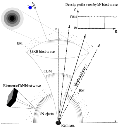
Figure 1: Schematic illustration of the model with GRB and kN BWs. Concentric circles in the top left part of the figure indicate the axial symmetry of the GRB and kN BWs The black box in the bottom left part of the figure indicates the discretization of the both ejecta types. The little black dots arranged along the GRB and kN BW outer surfaces indicate the constant density, static ISM. The possible trajectory for an elementary kN BW depend on whether it (i) avoids the CBM medium entirely (dotted line), (ii) moves behind the GRB BWs from the start (dashed line) interacting with the CBM, (iii) or enters the CBM region during/after GRB BW lateral expansion. For all three cases the schematic kN BW upstream density profile is shown in the upper right part of the figure, normalized to the ISM value. The system is observed off-axis.

When considering the interaction between kN and GRB BWs, we assume that the reverse shock has already crossed the GRB ejecta when the interaction starts. In other words, the density profile that kN BW encounter is generated by the forward shock within the GRB BW. We reiterate that we neglect the effect of GRB ejecta break out from the kN ejecta on the properties of the latter. Currently, such processes are studied with numerically expensive general-relativistic magnetohydrodynamics (GRMHD) simulations (e.g. Gottlieb et al., 2022) and are not well understood. We leave it to future work to assess how the GRB shock breakout change the kN afterglow.

The CBM density profile that kN BW interacts with depends on the properties of the GRB BW, as shown in Fig. 1. Specifically, when GRB BW are ultra-relativistic, the profile behind the shock front follows the Blandford & McKee solution Blandford & McKee (1976). When the BW decelerates to $\Gamma\simeq 1$, the downstream profile may be approximated with the Taylor-von Neumann-Sedov solution Sedov (1959). Since the kN BW is at most mildly relativistic, any interactions with the GRB BW will happen when the latter is slower, i.e., also mildly relativistic at most. Thus, we assume that the density profile that the kN BW encounters, moving behind the GRB BW is given by the Taylor-von Neumann-Sedov and reads

$$\rho_{\rm CBM}(r)=\rho^{\prime}\mathcal{D}(\eta),\hskip 5.69054pt\beta_{\rm CBM}(r)=\frac{2\beta_{\rm sh}\mathcal{V}(\eta)}{(\hat{\gamma}+1)},\hskip 5.69054ptP_{\rm CBM}(r)=p^{\prime}\mathcal{P}(\eta)\,,$$ (19)

where $\eta=r/R_{\rm sh}$, $\mathcal{D}$, $\mathcal{V}$, and $\mathcal{P}$ are given by equations (9), (10), and (11) in Book (1994). Here $R_{\rm sh}$, $\rho^{\prime}$, and $\beta_{\rm sh}$ denote the radius, density, and velocity at the shock computed with the formalism discussed above. We turn the Taylor-von Neumann-Sedov profile on when the GRB BW is slowed down to $\Gamma\sim 2$. Otherwise, if the kN BW moves behind the GRB one it experiences negligible upstream density, $\rho_{\rm CBM}\sim 0$. Since the GRB BW spreads laterally, it is possible that the kN one would enter the evacuated region later. For numerical reasons we assume that from the point of entry the $\rho_{\rm CBM}$ decreases exponentially, until the Taylor-von Neumann-Sedov profile takes over. Importantly, in our model we neglect the tail-on shock-shock collision itself, when two BWs catch up with each other.

Numerically, we solve the system of ordinary differential equations using explicit Runge-Kutta method of order $8(5,3)$ Prince & Dormand (1981). We include the adaptive step-size control as the system of ODEs becomes stiff, once kN ejecta enters the low-density environment.

2.2 Comoving synchrotron

In the previous derivation we implicitly assumed that BWs are not magnetized. However, as a BW moves through the ISM with small but finite magnetization, the magnetic fields may become amplified via several instabilities e.g., the current-driven instability Reville et al. (2006), the Kelvin-Helmholtz shear instability Zhang & Shu (2011), the Weibel (filamentation) instability Medvedev & Loeb (1999); Lemoine & Pelletier (2010); Tomita & Ohira (2016) the Čerenkov resonant instability Lemoine & Pelletier (2010), the Rayleigh-Taylor instability Duffell & MacFadyen (2013), the magneto-rotational instability Cerdá-Durán et al. (2011), or the pile-up effect Rocha da Silva et al. (2015). These processes are very complex and require high resolution, computationally expensive PIC and magnetohydrodynamics (MHD) simulations to study. In the GRB literature it is common to assume that a fixed fraction $\epsilon_{B}$ of the BW internal energy, $e^{\prime}=E_{\rm int}^{\prime}/V^{\prime}$, is deposited in random magnetic fields behind the shock, i.e., $B^{\prime}=\sqrt{8\pi\epsilon_{B}e^{\prime}}$. We assume $B^{\prime}$ to be constant behind the shock.

The incoming electrons gain energy while reflecting off and scattering on MHD instabilities present in collisionless shocks. At the scale of the electron’s gyro-radius, PIC simulations are employed to study particle dynamics (e.g. Sironi et al., 2015). At larger scales a coupled MHD-PIC approach is employed. However, the spatial and temporal extent of such simulations are still limited to a few $10^{3}$ of proton gyro-scales and few milliseconds Bai et al. (2015); Mignone et al. (2018). These studies show that the main process responsible for electron acceleration at collisionless shocks is the first-order Fermi acceleration Spitkovsky (2008); Sironi & Spitkovsky (2009, 2011); Park et al. (2015). Due to the complexity and computational cost of these simulations it is common to assume that a fixed fraction, $\epsilon_{e}$, of the internal energy is used for particle acceleration, while electrons, after the acceleration, follow a power-law distribution in energy, $dn_{e}/d\gamma_{e}\propto\gamma_{e}^{-p}$ with $\gamma_{e}$ being the electron LF, and $p$ being the spectral index Dermer & Chiang (1998); Sari et al. (1998).

First-principle simulations provide constraints on the microphysics parameters, $\epsilon_{B}$, $\epsilon_{e}$, and $p$. Specifically, for relativistic shocks $p{\simeq}2$, while for non-relativistic ones $p{\simeq}2.2$ Kirk & Duffy (1999); Keshet & Waxman (2005). (See Sironi et al. (2015); Marcowith et al. (2020) for recent reviews). Observations of GRB afterglows also provide constraints on these parameters, but the range is generally very broad Kumar & Zhang (2014). We treat them as free parameters of the model.

2.2.1 Comoving synchrotron from a GRB BW

The broken power law (BPL) electron spectrum has the following characteristic LFs. The maximum LF $\gamma_{e;\,\rm max}^{\prime}$ depends on how quickly an electron can gain energy in the acceleration process and how quickly it radiates it. In order to accelerate to a LF $\gamma_{e}^{\prime}$, an electron should not lose more than half of its energy to synchrotron radiation during the time required for acceleration. As the minimum time needed for electron acceleration is of the order of the Larmor time, $t_{L}=m_{e}c\gamma_{e}^{\prime}/q_{e}B^{\prime}$ Kumar & Zhang (2014)

$$\gamma_{e;\,\rm max}^{\prime}\simeq\sqrt{\frac{9m_{e}^{2}c^{4}}{8B^{\prime}q_{e}^{3}}}\,,$$ (20)

where $q_{e}$ and $m_{e}$ are the electron charge and mass.

Most of the electrons, however, are injected with $\gamma_{e;\,\rm min}^{\prime}$, which can be obtained from the normalization of the electron distribution function. For the case of a simple BPL and if $\gamma_{e;\,\rm max}^{\prime}\gg\gamma_{e;\,\rm min}^{\prime}$ as considered here, it can be obtained analytically (e.g. Kumar & Zhang, 2014)

$$\gamma_{e;\,\rm min}^{\prime}=\frac{p-2}{p-1}\frac{\epsilon_{e}e^{\prime}}{n^{\prime}m_{e}c^{2}}\,.$$ (21)

The cooling of electrons is driven by radiation losses and adiabatic expansion (e.g. Chiaberge & Ghisellini, 1999; Chiang & Dermer, 1999). Thus, at any point in time behind the shock there is a population of newly injected, “hot”, electrons and already partially cooled, “cold”, electrons. The exact evolution of the electron distribution function can be obtained by solving the continuity equation, the Fokker-Planck-type equation. This is however computationally expensive and in GRB afterglow literature it is common to consider the “fast” and “slow” cooling regimes of the electron spectrum approximated with BPLs, depending on whether $\gamma_{e;\,\rm min}^{\prime}$ is smaller or larger than a cooling LF $\gamma_{e;\,\rm c}^{\prime}$ defined as

$$\gamma_{e;\,\rm c}^{\prime}=\frac{6\pi m_{e}c}{\sigma_{T}t_{e}B^{\prime 2}\Gamma}\,,$$ (22)

where $\sigma_{T}$ is the Stefan-Boltzmann constant and $t_{e}$ is the emission time. Using Eqs. (20), (21) and (22), we compute the time evolution of the electron spectrum, approximated with the BPL. This spectrum, in turn, can be convolved with the synchrotron function Rybicki & Lightman (1986) to derive analytically the instantaneous synchrotron spectrum which itself is a BPL with critical frequencies: $\nu_{\rm min}^{\prime}(\gamma_{e;\,\rm min}^{\prime})$, $\nu_{\rm c}^{\prime}(\gamma_{e;\,\rm c}^{\prime})$, and $\nu_{\rm max}^{\prime}(\gamma_{e;\,\rm max}^{\prime})$ with varying degree of simplification (e.g. Sari et al., 1998; Dermer & Chiang, 1998; Wijers & Galama, 1999; Johannesson et al., 2006). We adopt the derivation of Johannesson et al. (2006) that approximates the synchrotron spectrum as a smooth BPL (their equations A1, A2, A6 and A7), that we recall here for completeness,

$$j_{\rm pl}^{\prime}(\nu^{\prime})= j_{\rm pl;\,max;\,f}^{\prime}\Bigg{[}\Big{(}\frac{\nu^{\prime}}{\nu_{c}^{\prime}}\Big{)}^{-\frac{\kappa_{1}}{3}}+\Big{(}\frac{\nu^{\prime}}{\nu_{c}^{\prime}}\Big{)}^{\frac{\kappa_{1}}{2}}\Bigg{]}^{-\frac{1}{\kappa_{2}}}$$ (23)

$$\times\Bigg{[}1+\Big{(}\frac{\nu^{\prime}}{\nu_{m}^{\prime}}\Big{)}^{\frac{(p-1)\kappa_{2}}{2}}\Bigg{]}^{-\frac{1}{\kappa_{2}}},$$

$$j_{\rm pl}^{\prime}(\nu^{\prime})= j_{\rm pl;\,max;\,s}^{\prime}\Bigg{[}\Big{(}\frac{\nu^{\prime}}{\nu_{m}^{\prime}}\Big{)}^{-\frac{\kappa_{1}}{3}}+\Big{(}\frac{\nu^{\prime}}{\nu_{m}^{\prime}}\Big{)}^{\frac{\kappa_{3}(p-1)}{2}}\Bigg{]}^{-\frac{1}{\kappa_{3}}}$$

$$\times\Bigg{[}1+\Big{(}\frac{\nu^{\prime}}{\nu_{c}^{\prime}}\Big{)}^{\frac{1}{2}\kappa_{4}}\Bigg{]}^{-\frac{1}{\kappa_{4}}},$$

for the fast and slow cooling, respectively. Here $j_{\rm pl}^{\prime}(\nu^{\prime})$ is the comoving emissivity from the power-law electron population at comoving frequency $\nu^{\prime}$. The characteristic frequencies are

$$\nu_{i}^{\prime}=\chi_{p}\gamma_{e;\,i}^{\prime 2}\frac{3B^{\prime}}{4\pi m_{e}c}\,,$$ (24)

and the $j_{\rm pl;\,max;\,f}^{\prime}$ and $j_{\rm pl;\,max;\,s}^{\prime}$ are the peak values of the spectrum for the fast and slow cooling regimes respectively, expressed as

$$j_{\rm pl;\,max;\,f}^{\prime} =2.234\phi_{p}\frac{q_{e}^{3}n^{\prime}B^{\prime}}{m_{e}c^{2}},$$ (25)

$$j_{\rm p;\,max;\,s}^{\prime} =11.17\phi_{p}\frac{p-1}{3p-1}\frac{e^{3}n^{\prime}B^{\prime}}{m_{e}c^{2}},$$ (26)

where, $\phi_{p}$, $\chi_{p}$, and $\kappa_{i}$ are fitting polynomials that capture the $p$-dependence Johannesson et al. (2006), and $n^{\prime}$ is the number density behind the shock front computed from the shock jump conditions (Sec. 2.1.3).

Using this formulation, we compute the synchrotron emission from a relativistic GRB BW. For completeness we compare it with other formulations available in the literature in App. A.

2.2.2 Comoving synchrotron from a kN BW

When a shock is ultra-relativistic $\Gamma_{\rm sh}\gg 1$ or non-relativistic $\beta_{\rm sh}\ll 1$ the synchrotron emission from a non-thermal population of electrons can explain observations of GRBs afterglows and SNRs, respectively Sari et al. (1998); Chevalier (1982). However, in the case of mildly relativistic shocks, $\Gamma_{\rm sh}\beta_{\rm sh}\sim 1$, numerical studies of electron acceleration at shocks show that most of the energy resides in the thermal electron population, i.e., electrons that follow thermal, Maxwell-Jüttner distribution function, and that the non-thermal (power-law) tail only contains a small fraction of the total post-shock energy Park et al. (2015); Crumley et al. (2019). Thermal electrons were shown to be important in explaining the peculiar steep optically-thin radio and mm spectra of the FBOT AT2018cow Ho et al. (2019b). But even before that, the thermal electron population was considered in application to GRBs afterglows Warren et al. (2018); Samuelsson et al. (2020); Giannios & Spitkovsky (2009); Ressler & Laskar (2017), and hot accretion flows Ozel et al. (2000). Recently, Margalit & Quataert (2021) (hereafter MQ21) presented an analytic formulation of the synchrotron radiation arising from the combined thermal and non-thermal populations of electrons taking into account the synchrotron self-absorption (SSA) in both populations and low-frequency corrections of emissivities. MQ21 considered a Maxwellian distribution function for thermal electrons and a power law for the non-thermal electrons.

The pitch-angle averaged emission and absorption coefficients can be expressed in terms of $x_{\rm M}=\nu^{\prime}/\nu_{\Theta}^{\prime}$, where $\nu_{\Theta}^{\prime}=3\Theta^{2}eB^{\prime}/4\pi m_{e}c$. For the thermal electron population emissivity and absorption coefficient read

$$j^{\prime}_{\nu^{\prime},\,\rm th}=\frac{\sqrt{3}q_{e}^{3}n^{\prime}B^{\prime}}{8\pi m_{e}c^{2}}\times\frac{2\Theta^{2}}{K_{2}(1/\Theta)}x_{\rm M}I(x_{\rm M})\,,$$ (27)

$$\alpha^{\prime}_{\nu^{\prime},\,\rm th}=\frac{\pi q_{e}n^{\prime}}{3^{3/2}\Theta^{5}B^{\prime}}\times\frac{2\Theta^{2}}{K_{2}(1/\Theta)}x_{\rm M}^{-1}I(x_{\rm M})\,,$$ (28)

where $\Theta$ is the dimensionless electron temperature, $\Theta=k_{B}T_{e}/m_{e}c^{2}$, $K_{2}(1/\Theta)$ is the modified Bessel function of second order, and $I(x_{\rm M})$ is the fitting function introduced in Mahadevan et al. (1996)

$$I(x_{\rm M})=\frac{4.0505a}{x_{\rm M}^{1/6}}\Big{(}1+\frac{0.40b}{x_{\rm M}^{1/4}}+\frac{0.5316g}{x_{\rm M}^{1/2}}\Big{)}\exp(-1.8899x_{\rm M}^{1/3})\,,$$ (29)

which describes the emissivity of the thermal population of electrons for small and large $x_{\rm M}$ Pacholczyk (1970); Petrosian (1981). The temperature-dependent coefficients $a$, $b$, $g$ are tabulated in Mahadevan et al. (1996) for $\Theta\in(0.084,5.40)$ or, equivalently, for $T\in(5\times 10^{8},3.2\times 10^{10})\,$K. These coefficients deviate from unity for $\Theta<5$ which is of relevance for the low-velocity elements of the kN ejecta or after the ejecta deceleration. Thus, we include this dependence in our implementation.

For the non-thermal electron population MQ21 considered the standard power-law spectrum $dn_{e}^{\prime}/d\gamma_{e}^{\prime}\propto\gamma_{e}^{\prime-p}$ with injection LF, $\gamma_{e,\,\rm min}^{\prime}$, equal to the mean LF of thermal electrons, $\gamma_{e;\,\rm min}^{\prime}=1+a(\Theta)\Theta$, where $a(\Theta)$ is the coefficient that varies between $3/2$ for non-relativistic electrons and $3$ for ultra-relativistic electrons and can be approximated as $a(\Theta)=6+15\Theta/(4+5\Theta)$ Ozel et al. (2000). Thus, the power-law distribution contains only supra-thermal electrons.

As ejecta continues to decelerate and $\gamma_{e;\,\rm min}^{\prime}\rightarrow 1$, it enters the so-called deep-Newtonian regime Sironi & Giannios (2013), that commences when $\beta_{\rm sh}\lesssim 8\sqrt{m_{p}/m_{e}}\bar{\epsilon}_{e}$, where $\bar{\epsilon}_{e}=4\epsilon_{e}(p-2)/(p-1)$ Margalit & Piran (2020). Synchrotron emission from electrons accelerated at lower velocity shocks is dominated by electrons with LF ${\simeq}2$, instead of those with $\gamma_{e;\,\rm min}^{\prime}$. This manifests as flattening of the LC at late times Sironi & Giannios (2013). Thus, when $\gamma_{e;\,\rm min}^{\prime}$ gets close to $1$, additional adjustments are needed. Specifically, we set that only a fraction of injected electrons, $\xi_{\rm DN}$, can contribute to the observed emission. The $\xi_{\rm DN}$ is computed according to Ayache et al. (2021) as

$$\xi_{\rm DN}=\frac{\gamma_{e;\,\rm max}^{\prime 2-p}-\gamma_{e;\,\rm min}^{\prime 2-p}}{\gamma_{e;\,\rm max}^{\prime 2-p}-1}\times\frac{\gamma_{e;\,\rm max}^{\prime 1-p}-1}{\gamma_{e;\,\rm max}^{\prime 1-p}-\gamma_{e;\,\rm min}^{\prime 1-p}}\,,$$ (30)

where $\gamma_{e;\,\rm max}^{\prime}$ is evaluated using Eq. (20).

The pitch-angle averaged synchrotron emissivity from non-thermal electrons reads (MQ21)

$$j_{\nu^{\prime};\,\rm pl}^{\prime}=C_{j}\frac{\epsilon_{e}}{\epsilon_{T}}\frac{q_{e}^{3}n^{\prime}B^{\prime}}{m_{e}c^{2}}g(\Theta)x^{-\frac{p-1}{2}}\,,$$ (31)

and the self-absorption coefficient is

$$\alpha_{\nu^{\prime};\,\rm pl}^{\prime}=C_{\alpha}\frac{\epsilon_{e}}{\epsilon_{T}}\frac{q_{e}n^{\prime}}{\Theta B^{\prime}}g(\Theta)x^{-\frac{p+4}{2}}\,,$$ (32)

where $C_{j}$ and $C_{\alpha}$ are $p$-dependent coefficients Rybicki & Lightman (1986); Mahadevan et al. (1996); Margalit & Quataert (2021), and $\epsilon_{T}$ is the fraction of shock energy that goes into thermal electrons.

We also implement the low-frequency corrections to the $j_{\nu^{\prime};\rm pl}^{\prime}$ and effect of the electron cooling following MQ21.

Thermal emissivity, $j^{\prime}_{\nu^{\prime},\rm th}$, decreases faster with velocity. Thus, post-deceleration spectrum is expected to be dominated by $j^{\prime}_{\nu^{\prime},\rm pl}$.

The total emissivity and absorption then read $j_{\nu^{\prime}}^{\prime}=j_{\nu^{\prime};\rm pl}^{\prime}+j_{\nu^{\prime};\rm th}^{\prime}$ and $\alpha_{\nu^{\prime}}^{\prime}=\alpha_{\nu^{\prime};\rm pl}^{\prime}+\alpha_{\nu^{\prime};\rm th}^{\prime}$, respectively.

2.3 Coordinate system

Both GRB and kN ejecta have angle dependent mass and velocity. We assume azimuthal symmetry, ie, ejecta properties depend on the polar angle only.

GRB ejecta is discretized into non-overlapping layers each of which has its own polar angle and initial LF, mass and energy. The polar angle, however, is not constant and evolves as BWs laterally expand.

kN ejecta is discretized into elements each of which has its own constant polar angle, initial LF and mass. They comprise shells of equal polar angle (i.e., they overlap) and layers of equal initial LF.

The coordinate system is implemented as follows.

Consider a spherical coordinate system $(R,\,\theta,\,\phi)$ where $R$ is the distance from the coordinate origin, and $\theta$ and $\phi$ are the latitudinal and azimuthal angles respectively. The central engine (post-merger remnant) is located at the coordinate origin, and the system’s symmetry axis ($z$-axis) lies along $\theta=0$. The observer is located in the $\phi=\pi/2$ plane and $\theta_{\rm obs}$ is the angle between the line of sight (LOS) and the $z$-axis. Thus, the unit vector of the observer is given by $\vec{n}_{\rm obs}=\big{(}0,\,\sin(\theta_{\rm obs})\vec{y},\,\cos(\theta_{\rm obs}\big{)}\vec{z})$.

We follow Lamb & Kobayashi (2017); Lamb et al. (2018); Fernández et al. (2021) and discretize each hemisphere into $k=\{1,2,...n-1\}$ rings centered on the symmetry axis plus the single central spherical cap, $k=0$. The spherical cap opening angle is $\theta_{l=1}$between two concentric circles on the sphere with $\theta_{l=i}$ and $\theta_{l=i+1}$. Setting the uniform distribution in terms of $\cos{(\theta_{l})}$, the $\theta_{l=i}=2\sin^{-1}\big{(}\sqrt{k/n}\sin(\theta_{\rm w}/2)\big{)}$, where $\theta_{\rm w}$ is the initial opening angle of the ejecta. For GRB ejecta it corresponds to the GRB opening angle (see Sec. 2.3.1). For kN ejecta it is set to $\pi/2$. Each ring of index number $j$ is discretized into $2i+1$ azimuthal regions bounded by $\phi_{ij}=2\pi j/(2i+1)$, where $j=\{0,1,2...i\}$. Overall, each ejecta shell is discretized into $\sum_{i=0}^{i=n-1}(2i+1)=n^{2}$ elements, each of which has a solid angle $2\pi\big{(}1-\cos{(\theta_{\rm w})}\big{)}/n^{2}$ Beckers & Beckers (2012). A specific element “c” then has coordinates $\theta^{\rm c}_{i},\phi^{\rm c}_{ij}$ with $\theta^{\rm c}_{i}=(\theta_{i}+\theta_{i+1})/2$ and $\phi^{\rm c}_{ij}=\phi_{ij}+\phi_{ij-1}/2$. The coordinate vector of the element is given by $\vec{v}_{ij}=R_{ij}\big{(}\sin{(\theta_{i})}\cos{(\phi_{ij})}\vec{x},\,\sin{(\theta_{i})}\cos{(\phi_{ij})}\vec{y},\,\cos{(\theta_{i})}\vec{z}\big{)}$, where $R_{ij}$ is the radius of the element. The angle between the LOS and the coordinate vector of the element

$$\cos{(\theta_{ij,\mathrm{LOS}})}=\sin{(\theta_{i})}\sin{(\phi_{ij})}\sin(\theta_{\rm obs})+\cos{(\theta_{i})}\cos(\theta_{\rm obs})\,.$$ (33)

Within this discretization, the GRB lateral spreading implies that each layer laterally expands with its own velocity given by Eq. (15). The interaction between layers is neglected, and the gradual pressure gradient expected for a lateral structure is approximated with a step-like function. This approximation leads to an overestimation of the lateral expansion. More importantly, since each of the layers interacts with the same upstream medium, collecting mass independently, the slowest BW will fall behind the faster ones. This method has been successfully applied to structured jet afterglow modelling Lamb et al. (2019b); Ryan et al. (2020); Fernández et al. (2021). However, its accuracy against numerical simulations of structured jets remains to be quantified in full detail.

2.3.1 GRB ejecta structure

Numerical simulations of jets, breaking out from either a stellar envelope (in the case of long GRBs) or BNS merger ejecta (in the case of short GRBs) show the presence of lateral structure, i.e., the flow properties depend on the angle from the polar axis De Colle et al. (2012); Xie et al. (2018); Gottlieb et al. (2020); Lamb et al. (2022). Such jets have a non-trivial afterglow behaviour, that depends strongly on the viewing angle Granot & Kumar (2003); Wei & Jin (2003); Zhang & Meszaros (2002); Rossi et al. (2004); Granot & Kumar (2003); Salafia et al. (2015); Lamb & Kobayashi (2017); Beniamini et al. (2020); Takahashi & Ioka (2021). Observations of GRB170817A also point towards a structured jet that was observed off-axis Fong et al. (2017); Troja et al. (2017); Margutti et al. (2018); Lamb & Kobayashi (2017); Lamb et al. (2018); Alexander et al. (2018); Mooley et al. (2018); Ghirlanda et al. (2019); Ryan et al. (2020). And among possible structure types, a Gaussian function is able to provide a good fit to GRB170817A (see however Lamb et al. (2020); Takahashi & Ioka (2021)). In a Gaussian jet, the initial energy per solid angle and LF of the jet read

$$E_{0}(\theta)=E_{\rm c}e^{-\theta^{2}/\xi_{1}\theta_{\rm c}^{2}},\,\Gamma_{0}(\theta)=1+(\Gamma_{\rm c}-1)e^{-\theta^{2}/\xi_{2}\theta_{\rm c}^{2}},\,$$ (34)

where $E_{\rm c}$, $\Gamma_{\rm c}$, and $\theta_{\rm c}$ are the energy, LF, and half-opening angle of the jet core, $\xi_{1}=1$ and $\xi_{2}=2$ are constants, set following Resmi et al. (2018); Lamb & Kobayashi (2017); Fernández et al. (2021).

2.3.2 kN ejecta structure

We consider dynamical ejecta profiles from a large set of NR BNS merger simulations targeted to GW170817 Perego et al. (2019); Endrizzi et al. (2020); Nedora et al. (2019); Bernuzzi et al. (2020); Nedora et al. (2021b); Nedora et al. (2021a); Cusinato et al. (2021). For all our simulations the ejecta data are publicly available. We focus on the list of simulations given in the Table (2) of N21. These simulations were performed with the general-relativistic hydrodynamics (GRHD) code WhiskyTHC Radice & Rezzolla (2012); Radice et al. (2014a, b, 2015). They include leakage and M0 neutrino schemes in optically thick and thin regimes respectively Radice et al. (2016, 2018c), and accounting for the turbulent viscosity of magnetic origin via an effective subgrid scheme Radice (2017, 2020). The importance of viscosity and advanced neutrino transport for obtaining more accurate dynamical ejecta properties is discussed in Radice et al. (2018b, c); Bernuzzi et al. (2020); Nedora et al. (2021b). Simulations are classified with their reduced tidal deformability $\tilde{\Lambda}$ and mass ratio $q$. The former is defined as (Favata, 2014),

$$\tilde{\Lambda}=\frac{16}{13}\frac{(M_{A}+12M_{B})M_{A}^{4}\Lambda_{A}}{M^{5}}+(A\leftrightarrow B)\,,$$ (35)

where $\Lambda_{i}\equiv 2/3\,C_{i}^{-5}k^{(2)}_{i}$ are the quadrupolar tidal parameters, $k_{i}^{(2)}$ are the dimensionless gravitoelectric Love numbers (Damour & Nagar, 2009), $C_{i}\equiv GM_{A}/(c^{2}R_{A})$ are the compactness parameters, and $i=A,B$. Here $A$, $B$ subscripts are used to label individual stars with individual gravitational masses $M_{A}$ and $M_{B}$, baryonic masses as $M_{b;\,A}$ and $M_{b;\,B}$. The total mass is $M=M_{A}+M_{B}$, and the mass ratio $q=M_{A}/M_{B}\geq 1$. Masses and velocities are given in units of ${\rm M_{\odot}}$ and $c$, respectively. All simulations were performed using finite temperature and composition-dependent nuclear EOSs. In particular, the following set of EOSs was considered: DD2 (Typel et al., 2010; Hempel & Schaffner-Bielich, 2010), BLh (Logoteta et al., 2021), LS220 (Lattimer & Swesty, 1991), SLy4 (Douchin & Haensel, 2001; Schneider et al., 2017), and SFHo (Steiner et al., 2013). Among them, DD2 is the stiffest (larger NS radii, larger tidal deformabilities and larger NS maximum supported masses), while SFHo and SLy4 are the softest.

As in N21 the ejecta kinetic energy distribution, $E_{k}=f(\Gamma,\theta)$ (that in turn depends on the binary parameters, $q$ and $\tilde{\Lambda}$) is used as the initial data for the afterglow calculation.

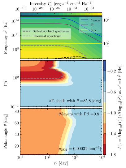
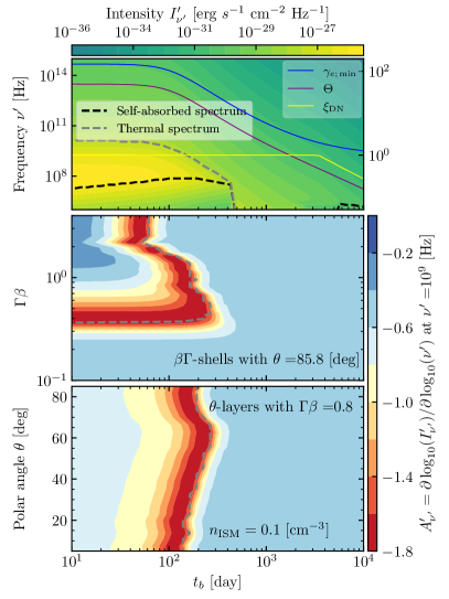
Figure 2: Top panels display the time evolution of the intensity in the frame comoving with the fluid produced by a single BW with initial momentum $\Gamma\beta=0.8$ and polar angle $\theta=85.8\,$deg (color-filled contours). The gray dashed line marks the location where the emission from thermal electron population is equal to that from the non-thermal. The black dashed line marks $\tau_{\nu^{\prime}}=1$. Also shown is the characteristic LF of the non-thermal electron distribution, $\gamma_{e;\,\rm min}^{\prime}$ (blue line); the fraction of electrons that are accelerated to the power-law distribution, $\xi_{\rm DN}$ (yellow line); and the dimensionless electron temperature, $\Theta$ (magenta line). Here $\xi_{\rm DN}=1$ imples that all injected electrons that are accelerated to the power-law distribution in energy contribute to the emission. Middle panels show the spectral index, $A^{\prime}_{\nu^{\prime}}$ at $1\,$GHz for all BWs with fixed $\theta=85.8\,$deg but varying initial momentum. Bottom panels show $A^{\prime}_{\nu}$ at $1\,$GHz for all BWs with different polar angles, $\theta$, but with the same initial momentum $\Gamma\beta=0.8$. The difference between the left and right panels is the ISM density, which is $0.00031\,\,\text{cm}^{-3}$ and $0.1\,\,\text{cm}^{-3}$ respectively. The plot shows that for fast ejecta with $\Gamma\beta>1$, the radio part of the spectrum, $\nu^{\prime}\simeq 1\,$GHz, is dominated by the emission from the thermal electron population. Meanwhile, at higher ISM density the contribution from thermal electron population is found in BWs with lower initial velocity.

2.4 Observed radiation

After all BWs corresponding to angular and velocity elements of GRB and kN ejecta are evolved, and comoving emissivities and absorption coefficients are obtained, the observed radiation is computed via equal time arrival surface (EATS) integration (e.g. Granot et al., 1999; Granot et al., 2008; Gill & Granot, 2018; van Eerten et al., 2010). For simplicity we first consider a given BW ($ij$) with its own angular position is computed. The retardation necessary for computing the emission from all BWs at a given observer time is discussed later in the section.

We consider plane parallel rays of varying impact parameters (perpendicular distances of rays to the central line of sight) through the emitting region Solving the radiation transport equation along these rays, we obtain Mihalas (1978)

$$\frac{\partial I_{\nu}}{\partial s}=j_{\nu}-\alpha_{\nu}I_{\nu}\,,$$ (36)

where $s$ is the line element along the ray.

The conversions of comoving emissivity and absorption coefficient into the observer frame read van Eerten et al. (2010): $j_{\nu}=j_{\nu}^{\prime}/(\Gamma(1-\beta\mu))^{2}$, $\alpha_{\nu}=\alpha_{\nu}^{\prime}(\Gamma(1-\beta\mu))$, where $\mu=\cos(\theta_{ij,\rm LOS})$ for a given BW. The transformation for the frequency reads $\nu^{\prime}=\nu(1+Z)\Gamma(1-\beta\mu)$, where $Z$ is the source redshift.

For the uniform plane-parallel emitting region the equation has an analytic solution

$$I_{\nu}=\frac{j_{\nu}}{\alpha_{\nu}}(1-e^{-\tau})\approxeq j_{\nu}\frac{3}{\tau}\Big{[}\frac{1}{2}+\frac{e^{-\tau}}{\tau}-\frac{1-e^{-\tau}}{\tau^{2}}\Big{]}\,,$$ (37)

where $\tau_{\nu}\approxeq-\alpha_{\nu}\Delta R/\mu^{\prime}$ is the optical depth with

$$\mu^{\prime}=\frac{\mu-\beta}{1-\beta\mu},$$ (38)

being the parameter relating the angle of emission in local frame to that in the observer frame Granot et al. (1999), accounting for cases when rays cross the homogeneous slab (ejecta) along directions different from radial. In the last equality in Eq. (37) we expressed the absorption coefficient as attenuation, following the equation $7.122$ in Dermer & Menon (2009).

The thickness of the emitting region, i.e., the region between the forward shock and the contact discontinuity of the BW in the observer frame reads, $\Delta R=\Delta R^{\prime}/(1-\mu\beta_{\rm sh})$ where $\Delta R^{\prime}=m_{2}/(2\pi m_{p}R^{2}(1-\cos(\omega))\Gamma n^{\prime})$ is obtained under the assumption of a homogeneous shell, but relaxing the assumption of the uniform upstream medium Johannesson et al. (2006). Notably, if $1-\cos(\omega)=2$ and the swept-up mass $m_{2}=4\pi R^{3}n^{\prime}m_{p}/3$, we recover the Blandford & McKee (BM) shock thickness, $\Delta R^{\prime}=R/12\Gamma^{2}$ (e.g. Johannesson et al., 2006; van Eerten et al., 2010).

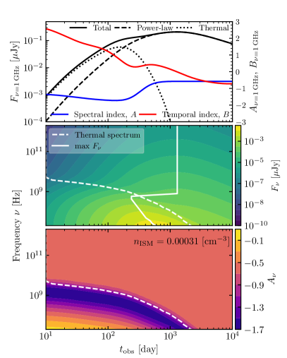
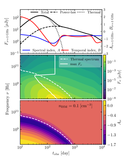
Figure 3: Top panels: afterglow LCs at $1\,$GHz, (black line) and the contributions from thermal electrons (dotted line) and non-thermal electrons (dashed line). Also shown is the spectral index, $A_{\nu}$, and the temporal index, $B_{\nu}$. Middle panels: evolution of the observed spectrum. Below the dashed white line the spectrum is predominantly thermal, i.e., is dominated by the emission from thermal electrons. The solid white line marks the frequency of peak flux. The intersection between the two white lines corresponds to the spectrum transition frequency, $\nu_{t}$. Bottom panels: time evolution of the spectral index, $A_{\nu}$, across all frequencies. The left and right panels are for low and high $n_{\mathrm{ISM}}$ respectively.

For a geometrically extended, evolving source, the observed radiation at a given frequency $\nu$ and at a given time $t_{\rm obs}$ is composed of many contributions from fluid elements emitting at various frequencies $\nu^{\prime}$ and at different times.

We compute the flux in the observer frame as piece-wise sum

$$F_{\nu}=\frac{1+Z}{2\pi d_{L}^{2}}\sum_{ij}R_{ij}(t_{ij,\rm obs})^{2}\Delta R_{ij}I_{ij,\nu}(t_{ij,\rm obs})\,,$$ (39)

where the arrival time, $t_{ij,\rm obs}$, for a given BW ($ij$) that corresponds to the $t_{\rm obs}$, is obtained via equation (4) of Fernández et al. (2021), and $d_{L}$ is the luminosity distance.

3 Results

3.1 Effects of thermal electrons on kN afterglow

3.1.1 Comoving emission

Here, we examine how the presence of thermal electrons affects the kN afterglow. We consider static, constant density ISM, $\rho_{\rm ISM}=n_{\rm ISM}m_{p}$, i.e., we neglect the presence of the GRB. We focus on the equal-mass BNS merger simulation with BLh EOS, as its ejecta profile has a fast tail that was closely examined in N21 (see their figure 3). For the remainder of this section we fix the following model parameters: $p=2.15$, $\epsilon_{e}=0.2$, and $\epsilon_{B}=0.005$. Following Margalit et al. (2022), we set $\epsilon_{T}=1$. The distance to the source is assumed to be $D_{\rm L}=41.3\,$Mpc, and it is observed at an angle of $\theta_{\rm obs}=30\,$deg. We consider two values for the ISM density, $n_{\rm ISM}=0.00031\,\,\text{cm}^{-3}$ and $n_{\rm ISM}=0.1\,\,\text{cm}^{-3}$.

In Fig. 2 we show the evolution of the intensity in the BW frame, $I_{\nu^{\prime}}^{\prime}(t_{b})$, for the two values of $n_{\rm ISM}$. Both thermal and non-thermal electron distributions are included. In the top panels of Fig. 2 we show $I_{\nu^{\prime}}^{\prime}(t_{b})$ for a single BW that corresponds to the ejecta element with polar angle $\theta=85.8\,$deg. and initial momentum $\Gamma_{0}\beta_{0}=0.8$. The choice is motivated by the fast tail angular distribution which is largely equatorial. At frequencies $\nu^{\prime}\gtrsim 1\,$GHz, $\nu^{\prime}\in(\nu_{\rm min}^{\prime},\nu_{\rm c}^{\prime})$, the spectrum is dominated by the emission from the non-thermal electron population. The spectral index, $A^{\prime}_{\nu^{\prime}}$, defined here as $A^{\prime}_{\nu^{\prime}}=d\log_{10}(I^{\prime}_{\nu^{\prime}})/d\log_{10}(\nu^{\prime})$, is $-0.575$ which corresponds to the electron spectral index $p=2.15$ and slow cooling regime. At very late times, $I_{\nu^{\prime}}^{\prime}(t_{b})$ declines as $\gamma_{e;\,\rm min}^{\prime}$ approaches unity and the fraction of electrons accelerated to the power-law distribution and contributing to emission, $\xi_{\rm DN}$, decreases. This decline in $I^{\prime}_{\nu^{\prime}}$ is seen at all frequencies, and it commences earlier for high upstream density.

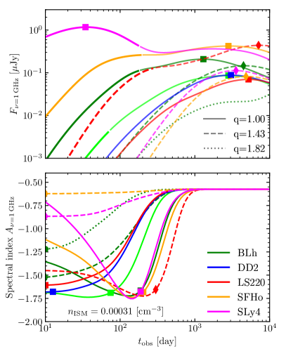
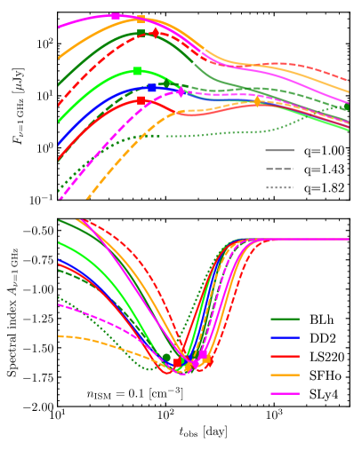
Figure 4: Top panels: Radio ($1\,$GHz) LCs for all simulations. Colors indicate different NS EOSs, and linestyles stand for various BNS mass ratio. Markers indicate the LC peak. Bottom panels: spectral index evolution. Markers indicate the spectral transition, $F_{\nu;\,\rm th}=F_{\nu;\,\rm pl}$. The difference between left and right panels is the same as in Fig.2, the observer angle $\theta_{\rm obs}=30\,$deg.

At early times and at low frequencies, $\nu^{\prime}\lesssim 1\,$GHz, $\epsilon_{\rm th}^{\prime}$ is larger than $\epsilon_{\rm pl}^{\prime}$. They are equal at the frequency marked by the dashed gray line, $\nu_{t}^{\prime}$, below which $\epsilon_{\rm th}^{\prime}>\epsilon_{\rm pl}^{\prime}$. We call this regime thermal. The frequency at which $\epsilon_{\rm th}^{\prime}=\epsilon_{\rm pl}^{\prime}$ depends primarily on the ejecta velocity, $n_{\rm ISM}$ and microphysical parameters, as illustrated in figure $2$ in MQ21.

Most known short GRBs with detected kN signatures occurred in low-density environments, $n_{\rm ISM}\ll 1\,\,\text{cm}^{-3}$ (e.g. Fong et al., 2017; Klose et al., 2019). Thus, under the assumption that $\epsilon_{T}=1$, we expect the transition in the spectrum to occur in the radio band. We focus the subsequent discussion on this part of the spectrum. Notably, for lower $\epsilon_{T}$, $\epsilon_{\rm th}^{\prime}$ and the transition frequency $\nu_{t}^{\prime}$ decreases. This behaviour is generic. We observe it in kN afterglows from other BNS merger simulations. At even lower frequencies, $\nu^{\prime}<\nu_{t}^{\prime}$, SSA becomes important. The region where $\tau_{\nu^{\prime}}>1$ is marked with black dashed line. Notably, even at high $n_{\rm ISM}$, e.g., $n_{\rm ISM}=0.1\,\,\text{cm}^{-3}$, the self-absorbed part of the spectrum lies below $100\,$MHz.

After the kN BW starts to decelerate and the electron temperature $\Theta$ decrease, the spectrum begins to change due to the steep dependence of $K_{2}(1/\Theta)$ on $\Theta$ (Eq. (27)). When $\Theta$ drops below ${\simeq}1$, at very late times, the corrections added to $I(x_{\rm M})^{\prime}$ (Eq. (29)) become important and the decrese in $\epsilon_{\rm th}^{\prime}$ becomes even steeper. Subsequently, the radio spectrum sharply transitions from thermal to non-thermal. This is seen in the top right panel of Fig. 2 as a cut-off of the gray curve at $t_{b}\simeq 3\times 10^{2}\,$days. At this time, the non-thermal electrons dominate the emission at all frequencies. The velocity dependence of $\epsilon_{\rm th}^{\prime}$ implies that different kN BWs with different initial momenta and energy produce different spectra that also evolves in time. In the middle panels of Fig. 2 the comoving spectral index, $A_{\nu^{\prime}}^{\prime}$ is shown as a function of the initial ejecta momentum. Notably, at $1\,$GHz, and $n_{\rm ISM}=0.00031\,\,\text{cm}^{-3}$ the spectrum is thermal only for BWs with initial momenta $\Gamma\beta\gtrsim 1$, i.e., for the ejecta fast tail, whereas at $n_{\rm ISM}=0.1\,\,\text{cm}^{-3}$, emission from thermal electrons is seen for $\Gamma\beta\gtrsim 0.4$.

The spectral index, $A_{\nu^{\prime}}^{\prime}$, and its temporal evolution as a function of the polar angle, $\theta$, for all BWs with initial momentum $\Gamma\beta=0.8$ are shown in the bottom panel of Fig. 2. As in the BNS simulations we consider, the fastest ejecta is found predominantly near the equatorial plane (being driven by core bounces Radice et al. (2018c); Nedora et al. (2021a)), and so the emission from thermal electrons is more important at $\theta\gtrsim 60\,$deg. This qualitative picture is characteristic for all ejecta in our BNS merger simulation set and hence might have important consequences for off-axis observations of BNS mergers.

3.1.2 Observed emission

For a single kN BW, the radio emission in the optically thin regime is characterised by the typical synchrotron frequency, $\nu_{\rm min}$. Using the BPL approximation to the synchrotron spectrum, the flux at $\nu_{\rm min}$ is $F_{\nu=\nu_{\rm min}}\propto R^{3}n_{\rm ISM}^{3/2}\epsilon_{B}^{1/2}\beta_{\rm sh}d_{L}^{-2}$, and while $\beta=$const, the flux increases. Thus, the LC peaks on the deceleration timescale of the BW Nakar & Piran (2011); Piran et al. (2013).

Combining the emission from all kN BWs, and accounting for relativistic effects, we display the evolution of the observed spectrum, $F_{\nu}(t_{\rm obs})$, in the middle panels of Fig. 3. The plot shows that as BWs decelerate, a progressively smaller part of the spectrum remains thermal (below the dashed white line). This is reflected in the evolution of the spectral index $A_{\nu}$, shown in the bottom panels of Fig. 3. There, the BW deceleration manifests as a decrease in the transition frequency in the spectrum. At a fixed frequency, however, an observer may trace the evolution of the spectral index and reconstruct the evolution of the BW speed. One would see a LC that is dominated by the emission from thermal electrons at first and later by the emission from non-thermal electrons, regardless of the ISM density. Notably, the relative brightness of these two types of synchrotron emission depends strongly on $n_{\rm ISM}$. As shown in Fig. 3, increasing $n_{\rm ISM}$ from $0.00031\,\,\text{cm}^{-3}$ to $0.1\,\,\text{cm}^{-3}$ leads to a rise in the flux density at $1\,\rm GHz$ from thermal and non-thermal electrons by four and two orders of magnitude, respectively (see top left and top right panels in the figure). Thus, if thermal electrons are indeed present behind kN shocks, their radio emission would be observable at early times. For instance, for $n_{\rm ISM}=0.1\,\,\text{cm}^{-3}$, the first, thermal LC peaks at a few $\mu$Jy, – slightly above the latest VLA upper limit for GRB170817A Balasubramanian et al. (2022). For lower values of $\epsilon_{T}$, the contribution from thermal electrons is smaller. Thus, the presence of thermal electron population can be inferred from (i) a double-peak structure of the LC and (ii) the characteristic evolution of the spectral index at early times. However, at early times the kN afterglow emission will likely be overshadowed by the GRB afterglow emission, unless the source is observed far off-axis.

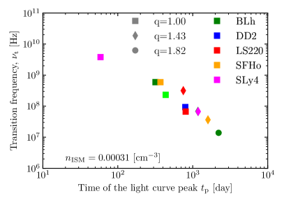
Figure 5: A relation between the frequency at which the spectrum transitions from being dominated by thermal electrons to the one dominated by non-thermal electrons, $\nu_{t}$, and the peak time, $t_{p}$, at this frequency. Colors indicate different NS EOSs, and markers stand for various values of the BNS mass ratio. Here, $n_{\rm ISM}=0.00031\,\,\text{cm}^{-3}$.

In Fig. 4 the kN afterglow LCs at $1\,$GHz are shown for all BNS simulations (top panel), as well as the evolution of the spectral index (bottom panel). At high density ($n_{\rm ISM}=0.1\,\,\text{cm}^{-3}$), the radio LCs display a distinct bimodal shape with maxima corresponding to the emission from thermal and later from non-thermal electrons. We call them thermal and non-thermal peak hereafter. A prominent exception is the highly asymmetric model with BLh EOS, in which the ejecta is of tidal origin only and lacks the fast tail Bernuzzi et al. (2020). The brightness and the peak time of the thermal peak are determined primarily by the ejecta velocity distribution and $n_{\rm ISM}$, and at sufficiently high $n_{\rm ISM}$, the LC overall peak is thermal. Otherwise, the peak is non-thermal. The large difference in spectral index, $-0.575$ for the non-thermal peak and ${\lesssim}-1.75$ for the thermal one, should permit distinguishing these scenarios. Similarly, if $n_{\rm ISM}$ is larger, so is the transition frequency, $\nu_{t}$. The relation between the transition frequency and the time of the LC overall peak at this frequency is shown in Fig. 5. Both, $\nu_{t}$ and $t_{p}$ depend on the model parameters and ISM density. However, we find that the relation depends only weakly on the $n_{\rm ISM}$ and microphysical parameters and is primarily determined by the ejecta velocity distribution. Indeed, equal mass models with soft EOSs always lie in the upper left corner, i.e., the spectral transition occurs at high frequencies, $\nu_{t}\gtrsim 1\,$GHz, and early in time. Meanwhile for highly asymmetric models the spectral transition occurs later and at lower frequency, $\mathcal{O}(50\,\rm MHz)$.

3.2 kN afterglow in the environment altered by a GRB BW

As discussed in Sec. 2.3.1, we consider a Gaussian jet, with parameters informed by observations and modelling of GRB170817A. Specifically, following Hajela et al. (2019) and Fernández et al. (2021), we set the jet half-opening angle $\theta_{\rm w}=15\,$deg. and core half-opening angle $\theta_{\rm c}=4.9\,$deg. The isotropic equivalent energy is $E_{\rm iso}=10^{52}\,$ergs, and the initial LF of the core is $\Gamma_{\rm c}=300$. The ISM density is set to $n_{\rm ISM}=0.00031\,\,\text{cm}^{-3}$, and the microphiscal parameters are set as: $\epsilon_{e}=0.05$, $\epsilon_{B}=0.0045$, and $p=2.16$. Luminosity distance to the source and the observer angle are set as $D_{\rm L}=41.3\,$Mpc, $\theta_{\rm obs}=21.5\,$deg, respectively. In the remainder of this section these parameters remain fixed unless stated otherwise.

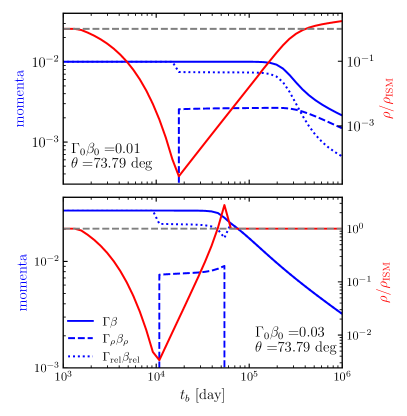
Figure 6: Dynamical evolution of the kN BW with initial momentum $\Gamma_{0}\beta_{0}$, moving at an angle $\theta$ through the CBM, i.e., the medium behind the laterally spreading GRB BW. The red lines denote the density of the CBM, immediately upstream of the kN BW. The solid blue line indicates the kN BW momentum, $\Gamma\beta$. The dashed blue line follows the momentum of the CBM upstream of the kN BW. The dotted blue line corresponds to the relative momentum between the CBM and kN BW. The gray line marks the $\rho_{\rm CBM}=\rho_{\rm ISM}$, i.e., $1$. For a low initial momentum (top panel), the kN BW stalls behind the overdensity at the forward shock of the GRB BW. Meanwhile, for a larger momentum kN BW successfully breaks through the overdensity (bottom panel).

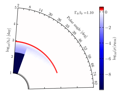
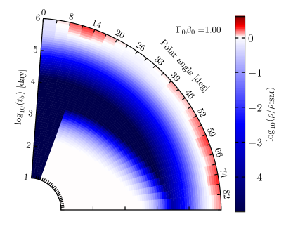
Figure 7: CBM density as seen by kN BWs with a given initial momentum, $\Gamma_{0}\beta_{0}=1.10$ on the left and $\Gamma_{0}\beta_{0}=1.00$ on the right. Blue color indicates densities below that of the ISM, which is typically found far behind the GRB BW. Red color indicates a density higher than $n_{\mathrm{ISM}}$, indicating that the kN BW caught up with the GRB BW.

Here, we recall the setup discussed in Sec. 2 and shown in Fig. 1. The GRB BW is moving through the ISM with a given number density, $n_{\rm ISM}$. A kN BW moves through either the ISM or the CBM (see Sec. 2.1.3), depending on whether the kN BW polar angle is larger or smaller than the GRB opening angle respectively.

In Fig. 6 we show, for two values of initial kN BW momentum, the dynamics of this BW moving behind the GRB BW, as well as the density profile that it encounters. In both cases, the kN BW moves outside of the GRB initial opening angle, $\theta>\theta_{\rm w}$, and thus encounters the ISM at the beginning. Later, when the GRB BW has spread, the kN BW enters the low-density region left by the passage of the GRB BW. Then the normalized upstream density, $\rho/\rho_{\rm ISM}$, exponentially decreases. Notably, if the density decreases faster than $\rho\propto R^{-3}$, the accumulated internal energy can be converted back into the bulk kinetic energy and re-accelerate the BW Shapiro (1980). In the case of a mildly relativistic, massive kN BW, however, this re-acceleration is negligible.

When the GRB BW slows down and the kN BW comes near, it starts to see the exponentially increasing density of the Taylor-von Neumann-Sedov profile, shown in Fig. 6 at $t_{b}\gtrsim 10^{4}\,$days. The upstream medium of the kN BW, however, moves with $\Gamma_{\rm CBM}\beta_{\rm CBM}$. The relative momentum, between the two is $\Gamma_{\rm rel}\beta_{\rm rel}$. When the distance between the BWs is large, both momenta remain relatively constant. The subsequent evolution depends strongly on the energy budget of the kN BW. A sufficiently fast BW can break through the overdense GRB BW. This scenario is shown in the bottom panel of the Fig. 6. The increase in $\Gamma_{\rm CBM}\beta_{\rm CBM}$ and decrease in $\Gamma_{\rm rel}\beta_{\rm rel}$ before this point are due to the onset of kN BW deceleration. However, if the kinetic energy of the kN BW is insufficient, it stalls and $\Gamma_{\rm CBM}\beta_{\rm CBM}$ becomes larger than $\Gamma_{\rm rel}\beta_{\rm rel}$, meaning that the kN BW bounced off. This scenario is shown in the top panel of Fig. 6.

Other BWs into which the kN ejecta is discretized follow similar evolutionary trajectories. Combined, they comprise the overall dynamics of the kN ejecta. In Fig. 7 the evolution of upstream density, $\rho/\rho_{\rm ISM}$ is shown as a function of the BW polar angle (fixing the BW initial momentum). At early times (before the lateral spreading of the GRB BW), kN BWs that have polar angle larger than the GRB opening angle ($\theta>\theta_{\rm w}$) propagate through ISM. At smaller polar angles ($\theta<\theta_{\rm w}$), the kN BWs move almost freely through the low-density CBM, indicated as a dark blue region in the figure. As the GRB BW decelerates and spreads, sweeping progressively larger amount of ISM at larger polar angles, it slows down even faster. Thus, a sufficiently fast kN BW at a large polar angle can avoid interacting with the GRB BW entirely. This is shown in the left panel of Fig. 7 where the density remain $\rho=\rho_{\rm ISM}$ throughout the evolution.

When mildly relativistic ejecta moves through cold ISM, strong shocks form naturally. When the ISM is pre-accelerated and pre-heated by the GRB BW, shock formation is not guaranteed. Thus, not every fluid element of the kN ejecta moving through CBM can form a BW. A sufficiently high sonic Mach number, $\mathcal{M}=\beta_{\rm REL}/c_{s}\gg 1$, the ratio of the relative bulk velocity to the sound speed, is required. The upstream sound speed is $c_{s}=\sqrt{\hat{\gamma}P/\rho}$, where $\hat{\gamma}$, $P$ and $\rho$ are the adiabatic index, pressure and density of the fluid. Margalit & Piran (2020) analytically showed that the flow of the kN ejecta far behind the GRB BW is subsonic, $\mathcal{M}<1$. However, right before the kN ejecta reaches the GRB BW, $\mathcal{M}$ rises to $\mathcal{M}\simeq 4$, and a “shock within a shock” can form. We confirm this picture on a qualitative level. Far behind the GRB BW, the density is low with respect to the pressure, and the sound speed is high, exceeding the relative speed of the kN ejecta ($\mathcal{M}<1$). Thus, kN ejecta move through the CBM without shocking it. However, close to the GRB BW, the density rises faster than the pressure, and for sufficiently fast part of kN ejecta the Mach number becomes $\mathcal{M}\gtrsim 1$ and shocks form. For slow elements of kN ejecta $\mathcal{M}$ remains below unity, shocks do not form and the ejecta fail to break through.

It is uncertain which minimum value of $\mathcal{M}$ is needed for the production of non-thermal electrons at the shock. First-order Fermi acceleration relies on electrons having a gyro-radius much larger than the shock thickness (which is of order of ion gyro-radius). This is referred to as “injection problem”; cf. Balogh & Treumann (2013) for a textbook discussion. Other mechanisms, such as shock drift acceleration or stochastic shock drift acceleration, were shown to energize electrons enough so they may participate in Diffusive Shock Acceleration (DSA) later Guo et al. (2014a, b); Kang et al. (2019); Kobzar:2021zyl; Amano & Hoshino (2022). Low-$\mathcal{M}$ shocks in, e.g., galaxy clusters are known to produce bright synchrotron radiation from non-thermal electrons, likely by re-acceleration of so-called “fossile” electrons Pinzke et al. (2013); Johnston-Hollitt (2017); Kang (2018). In the case of a GRB-kN system such high-energy electrons may naturally come from the GRB BW (Margalit & Piran, 2020). In this paper, we assume that when a flow is supersonic, synchrotron radiation is produced as described in Sec. 2.2.2.

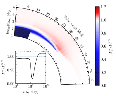
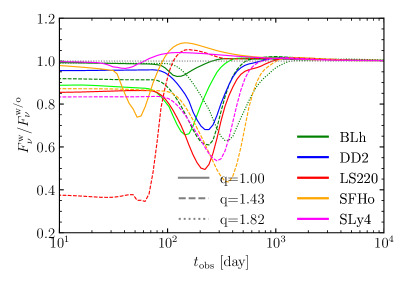
Figure 8: Left panel: Color-coded flux ratio at $\nu=1\,$GHz with (w) and without (w/o) accounting for the presence of CBM, introduced by the passage of GRB BW. The small bottom left panel displays the ratio of total LCs, integrating the emission from all kN BWs. Here, the ejecta profile with $q=1$ and the BLh EOS is used. Right panel: same LC ratio but for all simulations.

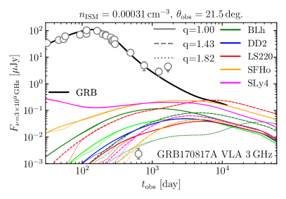
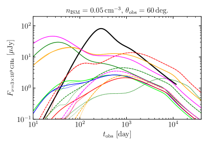
Figure 9: Radio ($3\,$GHz) LCs for all BNS merger models. Both, thermal and non-thermal electron populations are considered. LCs with smaller line width computed accounting for the presence of CBM. The GRB afterglow LC is shown with the black line alongside the observational data (Hajela et al., 2022; Balasubramanian et al., 2021, 2022). Left and right panels differ in the choice of $n_{\rm ISM}$ and $\theta_{\rm obs}$.

The effect of the GRB-altered CBM on the kN afterglow in terms of the ratio between the radio LCs computed with and without taking this alteration into account, $F_{\nu}^{\rm w}/F_{\nu}^{\rm w/o}$, is shown in Fig. 8. The qualitative behaviour of $F_{\nu}^{\rm w}/F_{\nu}^{\rm w/o}$ is similar to that suggested in Duran & Giannios (2015); Margalit & Piran (2020). Early emission is suppressed, $F_{\nu}^{\rm w}/F_{\nu}^{\rm w/o}<1$, due to the reduced CBM density and the low Mach number. The new aspect introduced here is the lateral spreading of the GRB BW and the dependency of the kN ejecta velocity on the polar angle. Indeed, $F_{\nu}^{\rm w}/F_{\nu}^{\rm w/o}$ depends on the angular profile of the kN ejecta, as the left panel of Fig. 8 illustrates. For equatorial ejecta the flux ratio remains close to unity, as most of the kN BWs either avoids interacting with post-GRB CBM entirely or passes through it too quickly to cause an appreciable change in the emission. Emission from polar ejecta is, however, largely suppressed at early times, and also later, if ejecta fails to form shocks and break through the overdensity behind the forward shock of the GRB BW. A minimum of $F_{\nu}^{\rm w}/F_{\nu}^{\rm w/o}$ is reached when most of the kN ejecta resides behind the GRB BW but have not produced a shock. At $\theta\gtrsim 45\,$ deg. the kN outflow is fast enough to break through or/and to excite a shock in the CBM, creating an appreciable excess in observed emission.

This behaviour is generic and found for other BNS models as well, as shown in Fig. 8 (right panel). If the fast tail of the kN ejecta is largely polar, as is the case for the model with LS220 EOS and $q=1.43$ (see figure 2 in N21), the flux suppression is more prominent and the minimum of $F_{\nu}^{\rm w}/F_{\nu}^{\rm w/o}$ is reached earlier. In general and across the models, however, the minimum of the flux ratio is seen at $t_{\rm FF;\,min}\approx 3\times 10^{2}\,$days. For simulations with soft EOSs and $q=1.0$ we find, on average, smaller $t_{\rm FF;\,min}$, and, conversely, a larger $t_{\rm FF;\,min}$ we find for models with stiff EOSs and $q>1$. This directly reflects the strength of the core bounce and the prominence of the fast tail in the ejecta velocity distribution. However, the emission suppression is generally below $40\,\%$, as the fast tail in all our models is largely equatorial and evolves in the ISM. The variation in flux is achromatic only if a single power-law electron distribution is assumed. In the presence of thermal electrons the spectral evolution is more complex due to steep dependency of $F_{\nu;\rm th}$ on the upstream density, as discussed in Sec. 3.1. The emission excess of up $10\,\%$ arises when kN ejecta shocks the CBM and is strongest in the model with SFHo EOS and $q=1.00$. For a spherical, uniform outflow (single-shell approximation) Margalit & Piran (2020) predicted the excess to be orders of magnitude larger and to be observable as “late-time radio flare”. We instead argue that the structure of kN ejecta as well as the finite spreading time of the GRB BW would smear the sharp peak and, depending on the details of the particle acceleration and synchrotron emission at $\mathcal{M}\gtrsim 1$ shocks, would produce a mild emission excess at most.

In Fig. 9 $3\,$GHz LCs are shown for both kN and GRB afterglows, for two values of $n_{\rm ISM}$ and $\theta_{\rm obs}$. LCs produced accounting for GRB-kN interaction are shown with thinner lines, and as expected, the difference with respect to those computed without including this interaction is minor and only present at early times. We reemphasize that free parameters of the kN afterglow model were not tuned to fit the observations. At ISM densities inferred for GRB170817A (left panel of Fig. 9), the kN afterglow emission from thermal electrons is at most as bright as the non-thermal emission and overall lies below the latest upper limits on GRB170817A radio emission Balasubramanian et al. (2022). Thus, the kN afterglow emission at early times is not bright enough to affect the total afterglow. At higher densities the emission from thermal electrons is significantly brighter, exceeding $10\,\mu$Jy. Additionally, as the fast tail of the kN outflow is largely equatorial, the early emission is further enhanced for a far off-axis observer. Meanwhile the GRB afterglow is dimmer, as the early emission from a collimated jet is beamed away from the observer LOS. Such a GRB afterglow, for which prompt emission also cannot be observed, is referred to as an orphan afterglow (e.g. Nakar et al., 2002; Ghirlanda et al., 2015; Huang et al., 2020). Thus, the presence of the kN afterglow may complicate the orphan afterglow signature and possibly contribute to the current non-detection of the GRB orphan afterglows.

4 Discussion & conclusion

One of the observables of BNS mergers is the kN afterglow. The mechanism behind this transient is similar to that of the GRB afterglow, but instead of a highly relativistic GRB ejecta, the mildly relativistic kN ejecta shocks the ambient medium and produces the emission (e.g. Nakar, 2020). The radio flux of the kN afterglow is expected to peak on the deceleration timescale, which is of the order of years. Its properties are determined primarily by the velocity and angular distribution of ejecta and unknown microphysical parameters, governing particle acceleration at mildly relativistic shocks. Thus, if detected, a kN afterglow could provide additional constraints on the ejecta properties, and specifically, on the fast component of the dynamical ejecta. Such information could be used to place additional constraints on the properties of merging NSs and the NS EOS. In N21 we considered GRB170817A which was accompanied by the kN AT2017gfo. Using the latest Chandra and VLA observations Balasubramanian et al. (2021); Hajela et al. (2022) and dynamical ejecta profiles from ab-initio NR BNS merger simulations with advanced input physics Radice et al. (2018c); Nedora et al. (2021b), we illustrated how such constraints can be placed. In this work we considered an impact on the kN afterglow of (i) a mixture of thermal and non-thermal electron populations producing synchrotron radiation, (ii) an upstream medium that is altered and pre-accelerated by the laterally spreading GRB BW.

Both observations and PIC simulations support the presence of a significant thermal electron population behind mildly relativistic shocks Park et al. (2015); Crumley et al. (2019); Ho et al. (2019a); 2021MNRAS.502.5065L. We find that the emission from this population can dominate the early kN afterglow in radio band. At sufficiently high densities, $n_{\rm ISM}\simeq 0.1\,\,\text{cm}^{-3}$, radio LCs can have a double-peak structure. The strong velocity dependence of the emissivity from thermal electrons leads to a characteristic evolution of the spectra as the fastest kN BWs decelerate and the contribution from thermal electron population to overall emission decreases. Thus, a characteristic increase in the spectral index in the radio band may be used to constrain the ejecta velocity distribution. Additionally, we find a relation between the time of the LC peak and the frequency at which one observes the transition of the spectrum from being dominated by the emission from thermal electrons to the one dominated by the emission from non-thermal electrons. This relation depends only weakly on microphysical parameters and $n_{\rm ISM}$, and thus can be used to constrain the presence of the fast tail in the ejecta velocity distribution.

At densities similar to those inferred for GRB170817A, we find the kN afterglow in the radio band ($3\,$GHz) peaking at $10^{3}-10^{4}\,$days, reaching a flux $\lesssim 0.1\,\mu$Jy, which is below the latest upper limits Balasubramanian et al. (2022). However, as the LC peak flux depends strongly on the microphysics of the shock, we cannot place stringent constraints in this case. At higher ISM densities the early kN afterglow may be observable at the distance of GRB170817A but it would be overshadowed by the GRB afterglow, unless observed far off-axis. There, GRB orphan afterglow and kN afterglow are comparably bright. Thus, kN afterglow may be an important factor in search strategies for GRB orphan afterglows.

As GRB and kN ejecta move through the same environment, it is natural to expect that the former would affect the kN afterglow. Here we considered how the dynamics of and the radiation from kN BWs change when they move through the CBM with density profile dependent on the position and properties of the laterally spreading GRB BW ahead. The early kN afterglow is slightly (${\lesssim}20\,\%$) dimmer due to the lower CBM density (with respect to the ISM) behind the GRB BW. Later, lateral spreading of the GRB BW increases the area of low-density, pre-accelerated CBM through which kN outflow moves subsonically. This implies a more significant reduction in observed flux (${\lesssim}40\,\%$), followed by a slight brightening (${\lesssim}10\,\%$), when the kN flow excite shocks in the overdense part of the CBM at the GRB BW. Thus, early-time variability in kN afterglow LCs, besides the spectral evolution, may also be present due to the interaction with the modified upstream medium, albeit the former has a much stronger effect. If, on the other hand, the kN ejecta velocity distribution is such that the fastest outflow is polar instead of equatorial, the suppression of emission might be much more significant, and, potentially, observable. Moreover, a system of two mildly relativistic shocks, one approaching another is an interesting and, to the best of our knowledge, unexplored setting for particle acceleration and synchrotron emission with seed particles.

The main limitations of our study relate to the semi-analytic models of GRB and kN afterglows. It remains to be investigated whether the qualitative results presented here would also be found in numerical hydrodynamics simulations. Such simulations, however, even with novel techniques like moving mesh Xie et al. (2018); Akcay et al. (2019), are numerically expensive. Additionally, the theory of particle acceleration at mildly relativistic shocks with very heavy ions, (produced in $r$-process) is currently not well understood. This limits our ability to predict the properties of kN afterglows. Nevertheless, our improved capability to localize off-axis GRBs using GW detectors and the improved sensitivity of new radio observatories would allow us in the near future to follow these GRBs for longer, and to place constraints on the kN afterglow properties and physical processes operating at shocks.

Data avalibility

The data underlying this article will be shared on reasonable request to the corresponding author.

Appendix A Synchrotron spectrum approximants

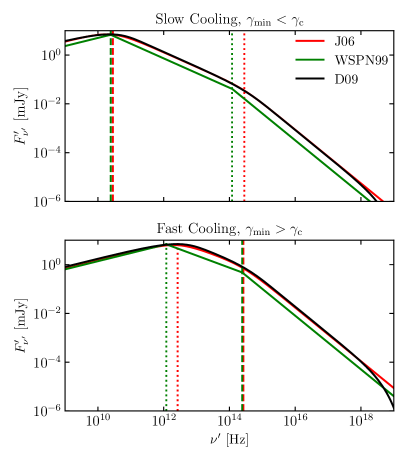
Figure 10: Comparison between several approximants to the synchrotron radiation from power-law distribution of electrons with $p=2.2$, $\gamma_{e;\,\rm min}^{\prime}=10^{2}$, $\gamma_{e;\,\rm c}^{\prime}=10^{4}$ in the magnetic fields $B=1\,$G. The emitting region has radius $R=10^{12}\,$cm, mass $m_{2}=10^{20}\,$g, moving through the ISM with number density $n_{\rm ISM}=10^{-1}\,\,\text{cm}^{-3}$. We compare the BPL approximants from Johannesson et al. (2006) (red line); from Sari et al. (1998) and Wijers & Galama (1999) (green line); and numeric integration of the approximated synchrotron function from Dermer & Menon (2009) (black line).

Several approximants to the synchrotron emission from a power law distribution of electrons exist in the literature. In the main text we focused on the formulation proposed by Johannesson et al. (2006) for GRB afterglows, that we label as J06 in this section. To motivate this choice we compare this formulation with widely used model by Sari et al. (1998) and with more direct integration of a synchrotron function Rybicki & Lightman (1986) given in Dermer & Menon (2009). In the former, the comoving emissivity is given as

$$j_{\rm pl}^{\prime}(\nu^{\prime})=j_{\rm pl;\,max}^{\prime}\begin{cases}\Big{(}\frac{\nu^{\prime}}{\nu_{\rm min}^{\prime}})^{1/3}\text{ if }\nu^{\prime}<\nu_{\rm min}^{\prime}\,,\\ \Big{(}\frac{\nu^{\prime}}{\nu_{\rm min}^{\prime}}\Big{)}^{(1-p)/2}\text{ if }\nu_{\rm min}^{\prime}<\nu^{\prime}<\nu_{\rm c}^{\prime}\,,\\ \Big{(}\frac{\nu^{\prime}}{\nu_{\rm min}^{\prime}}\Big{)}^{(1-p)/2}\Big{(}\frac{\nu^{\prime}}{\nu_{\rm c}^{\prime}}\Big{)}^{-p/2}\text{ if }\nu^{\prime}>\nu_{\rm c}^{\prime}\,,\end{cases}$$ (40)

in the slow cooling regime and

$$j_{\rm pl}^{\prime}(\nu^{\prime})=j_{\rm pl;\,max}^{\prime}\begin{cases}\Big{(}\frac{\nu^{\prime}}{\nu_{\rm c}^{\prime}})^{1/3}\text{ if }\nu^{\prime}<\nu_{\rm c}^{\prime}\,,\\ \Big{(}\frac{\nu^{\prime}}{\nu_{\rm c}^{\prime}}\Big{)}^{-1/2}\text{ if }\nu_{\rm c}^{\prime}<\nu^{\prime}<\nu_{\rm min}^{\prime}\,,\\ \Big{(}\frac{\nu_{\rm c}^{\prime}}{\nu_{\rm min}^{\prime}}\Big{)}^{-1/2}\Big{(}\frac{\nu^{\prime}}{\nu_{\rm c}^{\prime}}\Big{)}^{-p/2}\text{ if }\nu^{\prime}>\nu_{\rm min}^{\prime}\,,\end{cases}$$ (41)

in the fast cooling regime. In the calculation of the spectral breaks and $j^{\prime}_{\rm pl;\,max}$ the integration over the emission angle has to be included which gives a correction factor of $3/4\pi$ Wijers & Galama (1999). Then, the spectral breaks read

$$\nu_{\rm min}^{\prime}=\chi_{p}\frac{3}{4\pi}\gamma_{e;\,\rm min}^{2}\frac{q_{e}B^{\prime}}{m_{e}c}\,,$$ (42)

and

$$\nu_{\rm c}^{\prime}=0.286\frac{3}{4\pi}\gamma_{e;\,\rm c}^{2}\frac{q_{e}B^{\prime}}{m_{e}c}\,.$$ (43)

The maximum of the spectrum is

$$j_{\rm pl;\,max}^{\prime}=\phi_{p}\sqrt{3}\frac{q_{e}^{3}B^{\prime}}{m_{e}c^{2}}\,,$$ (44)

where $\chi_{p}$ and $\phi_{p}$ are electron spectrum dimensionless maximum and corresponding dimensionless flux. They account for the isotropic distribution of angles between the electron velocity and the magnetic field. They are tabulated in Wijers & Galama (1999). We label this formulation as WSPN99 in Fig. 10.

In Dermer & Menon (2009) approximations to modified Bessel functions are provided for a more numerically efficient calculation of a synchrotron emission from an arbitrary electron distribution. We consider the BPL electron distribution,

$$n_{e}(\gamma^{\prime})= k_{e}\Bigg{[}\left(\frac{\gamma_{e}^{\prime}}{\gamma^{\prime}_{e;\,\rm c}}\right)^{-p_{1}}\,H(\gamma_{e}^{\prime};\gamma^{\prime}_{e;\,\rm min},\gamma^{\prime}_{e;\,\rm c})$$ (45)

$$+\left(\frac{\gamma_{e}^{\prime}}{\gamma^{\prime}_{e;\,\rm c}}\right)^{-p_{2}}\,H(\gamma_{e}^{\prime};\gamma^{\prime}_{e;\,\rm c},\gamma^{\prime}_{e;\,\rm max})\Bigg{]}\,,$$

where $k_{e}$ is the spectral normalization, $H(...)$ is the Heaviside step function, $p_{1}=p$ if $\gamma_{e;\,\rm min}^{\prime}<\gamma_{e;\,\rm c}^{\prime}$ and $p_{1}=2$ otherwise, $p_{2}=p+1$, accounting for the slow and fast cooling regimes respectively. The angle-averaged integrand of the radiated power, $R(x)$, is approximated with equation D7 of Aharonian et al. (2010) where the ratio of the frequency to the critical synchrotron frequency, $x$, is computed with equation 7.34 in Dermer & Menon (2009). We label this formulation as D09 in Fig. 10 and consider it as a reference point.

Comparing the spectra, we observe that while the spectral peaks and slopes in different regimes are captured by the analytic approximants, WSPN99 and D09, the value of the flux density $F_{\nu^{\prime}}^{\prime}$ between the spectral breaks is generally underestimated by the WSPN99 formulation. In PyBlastAfterglow, where radiation from a large number of BWs in combined to obtain the observed flux, this might lead to lower fluxes. Meanwhile, the spectra produced by J06 formulation is in a good agreement with the reference, especially in the slow cooling regime which is of prime importance for this work. Thus, due to the high computational efficiency of analytic methods, we consider J06 formulation in the main text.

Appendix B Blastwave dynamics approximants

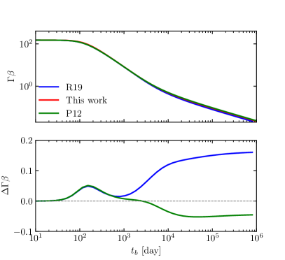
Figure 11: Dynamical evolution of a BW with $\Gamma_{0}=150$, $E_{0}=10^{52}\,$erg, and half-opening angle, $\theta_{0}=0.1\,$rad propagating through $n_{\rm ISM}=10^{-3}\,\,\text{cm}^{-3}$. The red line indicates to the evolution computed with PyBlastAfterglow, Eq. (14). The while blue line corresponds to the model of Ryan et al. (2020). The green line denotes the formulation of Pe’er (2012). The relative difference is shown in the bottom panel.

There are several formulations for the dynamics of a transrelativistc BW propagating through a cold ISM under the “thin-shell” approximation in the literature. It is instructive to compare the evolution of a BW computed with PyBlastAfterglow with other formulations in the literature. First, we consider the formulation proposed by Pe’er (2012), where the adiabatic losses are neglected which we label here P12. The evolution equation for the bulk LF for P12 reads

$$\frac{d\Gamma}{dm_{2}}=\frac{-(\hat{\gamma}(\Gamma^{2}-1)-(\hat{\gamma}-1)\Gamma\beta^{2})}{M_{0}+m_{2}(2\hat{\gamma}\Gamma-(\hat{\gamma}-1)(1+\Gamma^{-2}))}\,,$$ (46)

where $M_{0}$ is the initial mass of the fireball and $m_{2}$ is the swept-up mass. The adiabatic index, $\hat{\gamma}$, is computed with the same, Eq. (2), as in PyBlastAfterglow.

Additionally, we consider the formulation proposed by Ryan et al. (2020) that is implemented in the publicly available code afterglowpy. There, the EOS is the “TM” variant presented in Mignone et al. (2005). We label this formulation as R19 in the Fig. (11).

Overall, the evolution of a BW consists of three stages: free-coasting, deceleration in the Blandford & McKee regime and deceleration in the Taylor-von Neumann-Sedov regime. Both the R19 and the P12 formulations display these stages and show an overall good agreement with PyBlastAfterglow at early times. At late times, however, there is a small discrepancy, given primarily by the different EOS, when comparing with R19 and different treatment of the internal energy transformation when comparing with the P12 formulation.

Appendix C Blastwave lateral expansion approximants

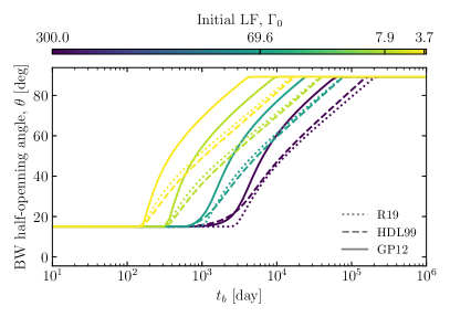
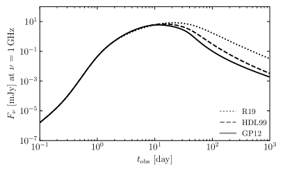
Figure 12: Top panel: evolution of the BW half-opening angle for several initial LFs (color-coded). Several lateral expansion prescriptions are considered. The solid line denotes $d\omega/dR$ from Granot & Piran (2012), The dashed line denotes the model of Huang et al. (2000) and the dotted line corresponds to the prescription from Ryan et al. (2020). The color of the line indicate the initial LF of the BW. Bottom panel: radio LCs for a top-hat jet observed off-axis, $\theta_{\rm obs}=0.16$, for the three aforementioned lateral spreading prescriptions. Geometry and microphsyics of the GRB model are discussed in Sec. D.

In most semi-analytic models of the BW evolution that employ the thin-shell approximation, lateral spreading cannot be incorporated in a self-consistent way (see, however Lu et al. (2020)). Here we compare the lateral spreading prescription from Granot & Piran (2012), the default option in PyBlastAfterglow, with other prescriptions available in the literature (and implemented in PyBlastAfterglow).

Lateral expansion is determined by the co-moving sound speed, $c_{s}^{2}=dp^{\prime}/de^{\prime}|_{s}$, at a shock Kirk & Duffy (1999)

$$c_{s}^{2}=\frac{\hat{\gamma}p^{\prime}}{\rho^{\prime}}\Big{[}\frac{(\hat{\gamma}-1)\rho^{\prime}}{(\hat{\gamma}-1)\rho^{\prime}+\hat{\gamma}\rho^{\prime}}\Big{]}c^{2}=\frac{\hat{\gamma}(\hat{\gamma}-1)(\Gamma-1)}{1+\hat{\gamma}(\Gamma-1)}c^{2}\,,$$ (47)

where in the last equation we expressed $\hat{\gamma}$ through the EOS, Eq. (2).

Assuming that the expanding fluid element interacts only with its immediate vicinity, the lateral and radial components of the velocity are related as $\beta_{r}/\beta_{\omega}=\partial\omega/\partial\ln R$. Furthermore, assuming that the spreading proceeds at the sound speed, $\upsilon_{\omega}=c_{s}$, the lateral expansion can be written as Huang et al. (2000)

$$\frac{d\omega}{dR}=\frac{\upsilon_{\omega}}{R\Gamma\beta c}\,.$$ (48)

This formulation, labeled as HDL99, has been broadly used in the early semi-analytic GRB afterglow models (e.g. Rossi et al., 2004).

More recently, Ryan et al. (2020) proposed a “conical” spreading model, where at a given time, all material that has been swept up affects the spreading. The tangential component of the velocity then reads

$$\upsilon_{\perp}=c\Gamma\sqrt{(1-\beta\beta_{\rm sh})c_{2}^{2}-(\beta_{\rm sh}-\beta)^{2}}$$ (49)

where both $c_{s}^{2}$ and $\beta_{\rm sh}=\dot{R_{\rm sh}}$ are evaluated using the “TM” EOS Mignone et al. (2005). The spreading is allowed once $\Gamma\beta>1/(3\sqrt{2}\omega_{\rm c})$, where $\omega_{\rm c}$ is the half-opening angle of the jet core. The spreading is given as $\dot{\omega}=\upsilon_{\perp}/R$. We label this prescription as R19.

The result of the comparison is shown in Fig. 12 for several GRB layers with different initial LFs, $\Gamma_{0}$ (top panel). The difference in LCs for an off-axis top-hat jet discussin in the next section, Sec. D, are shown in the bottom panel of the figure. For the largest $\Gamma_{0}$, for all prescriptions, the lateral spreading starts smoothly when the BW enters mildly relativistic regime. For low values of $\Gamma_{0}$, however, the onset of spreading is sharp, as sound speed is relatively low.

The subsequent evolution of the BW half-opening angle proceeds similar for the HDL99 and the R19 formulations. Notably, we did not use the final equation for $d\omega/dR$ from Ryan et al. (2020), as it implicitly assumes the “TM” EOS, that is different from the one adopted here. Moreover, the formulation designed in that work is tailored to the specific structured model and jet discretization, that differs considerably from the one used in PyBlastAfterglow. This contributes to the large difference in radio LCs. The lateral spreading computed with GP12 formulation proceeds faster. Fast spreading has been observed in the number of numerical studies of jet spreading Xie et al. (2018); van Eerten et al. (2010); Granot & Piran (2012); Duffell et al. (2018). It results in a reduced late time emission, as the faster spreading leads to larger accreted mass and earlier BW deceleration. As this formulation has been used in semi-analytic models with similar jet structure and discretization as ours Fernández et al. (2021), we employ it as a default option. Additionally, we find that qualitative results discussed in the main text do not depend on the exact formulation of the lateral spreading.

Appendix D GRB afterglow comparison with afterglowpy

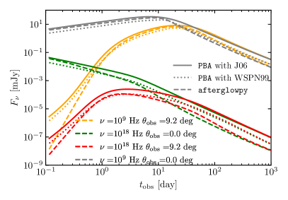
Figure 13: Comparison between LCs from a top-hat jet between PyBlastAfterglow with two different synchrotron radiation approximations (sold and dotted lines) and afterglowpy. This is analogous to the figure 2 of Ryan et al. (2020).

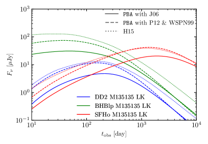
Figure 14: Comparison between kN afterglow LCs, computed with PyBlastAfterglow (using two different input physics settings, denoted with the solid and dashed lines) and the afterglow code of Hotokezaka & Piran (2015). The ejecta profiles from three NR simulations, presented in Radice et al. (2018c) (see their figures 30 and 31) were used.

Here we compare the GRB afterglow LCs generated with PyBlastAfterglow and those computed with afterglowpy. As in the latter the analytic synchrotron radiation formulation of Sari et al. (1998) was is, we compare LCs computed using the WSPN99 and the J06 formulations (see Sec. A) separately. The GRB parameters are: $\Gamma_{0}=150$, $E_{\rm iso}=10^{52}\,$ergs, $\theta_{\rm w}=0.1\,$rad, $n_{\rm ISM}=10^{-3}\,\,\text{cm}^{-3}$, $\epsilon_{e}=0.1$, $\epsilon_{b}=0.001$, $p=2.2$, $d_{\rm L}=3.09\times 10^{26}\,$cm, and $z=0.028$.

The result is shown in Fig. 13. Overall we find a reasonably good agreement between the LCs produced with PyBlastAfterglow and afterglowpy. The differences stem largely from different EATS integration methods. Especially, at early times, as the GRB is observed off-axis. At late times the differences in dynamics formulations (see Sec. B) also contribute.

Appendix E Method comparison for kN afterglow

In this section we compare kN afterglow LCs computed with PyBlastAfterglow and with the code of Hotokezaka & Piran (2015). We label the latter as H15. Specifically, we consider ejecta profiles from three NR BNS merger simulations, described in Radice et al. (2018c), the radio LC for which are shown in figures 30 and 31 in that work. The data for these simulations is publicly available. To the best of our knowledge, this is the first direct comparison between two different models for kN afterglows. Although, these models are semi-analytic and approximate, such comparisons are necessary in order to assess systematic uncertainties. However, no detailed information regarding the BW dynamics formulation and EATS integration procedure are available in Hotokezaka & Piran (2015). Comparing the radio LCs, shown in Fig. 14, we observe that the overall LC shape and the time of the peak are well reproduced by PyBlastAfterglow. This implies that the dynamics of different ejecta elements is similarly modelled. However, LCs computed with PyBlastAfterglow are systematically dimmer, especially if the J06 formulation for synchrotron radiation is used. The best agreement is found when the P12 formulation for dynamics (see Sec. B), and the WSPN99 formulations for radiation (see Sec. A) are used. The remaining discrepancy may stem from different EATS integration methods.

References

- Abbott et al. (2017) Abbott B. P., et al., 2017, Astrophys. J. Lett., 848, L13
- Abbott et al. (2018) Abbott B., et al., 2018, Living Rev. Rel., 21, 3
- Aharonian et al. (2010) Aharonian F. A., Kelner S. R., Prosekin A. Y., 2010, Physical Review D, 82, 043002
- Aharonian et al. (2013) Aharonian F., et al., 2013
- Ajello et al. (2016) Ajello M., et al., 2016, Astrophys. J., 819, 44
- Akcay et al. (2019) Akcay S., Bernuzzi S., Messina F., Nagar A., Ortiz N., Rettegno P., 2019, Phys. Rev. D, 99, 044051
- Alexander et al. (2017) Alexander K. D., et al., 2017, Astrophys. J., 848, L21
- Alexander et al. (2018) Alexander K., et al., 2018, Astrophys. J., 863, L18
- Amano & Hoshino (2022) Amano T., Hoshino M., 2022, Astrophys. J., 927, 132
- Arcavi et al. (2017) Arcavi I., et al., 2017, Nature, 551, 64
- Arnett (1982) Arnett W. D., 1982, The Astrophysical Journal, 253, 785
- Ayache et al. (2021) Ayache E. H., van Eerten H. J., Eardley R. W., 2021, Mon. Not. Roy. Astron. Soc., 510, 1315
- Bai et al. (2015) Bai X.-N., Caprioli D., Sironi L., Spitkovsky A., 2015, Astrophys. J., 809, 55
- Balasubramanian et al. (2021) Balasubramanian A., et al., 2021, Astrophys. J. Lett., 914, L20
- Balasubramanian et al. (2022) Balasubramanian A., et al., 2022
- Balogh & Treumann (2013) Balogh A., Treumann R. A., 2013, Physics of Collisionless Shocks. Space Plasma Shock Waves, Springer-Verlag New York Inc., https://link.springer.com/book/10.1007/978-1-4614-6099-2
- Barnes et al. (2016) Barnes J., Kasen D., Wu M.-R., Martínez-Pinedo G., 2016, Astrophys. J., 829, 110
- Bauswein et al. (2013) Bauswein A., Goriely S., Janka H.-T., 2013, Astrophys.J., 773, 78
- Beckers & Beckers (2012) Beckers B., Beckers P., 2012, Computational Geometry, 45, 275
- Beloborodov (2002) Beloborodov A. M., 2002, eConf, C0208122, 4
- Beloborodov (2008) Beloborodov A. M., 2008, AIP Conf. Proc., 1054, 51
- Beniamini et al. (2020) Beniamini P., Granot J., Gill R., 2020, Mon. Not. Roy. Astron. Soc., 493, 3521
- Berger et al. (2013) Berger E., Fong W., Chornock R., 2013, Astrophys. J. Lett., 774, L23
- Bernuzzi (2020) Bernuzzi S., 2020, Gen. Rel. Grav., 52, 108
- Bernuzzi et al. (2020) Bernuzzi S., et al., 2020, Mon. Not. Roy. Astron. Soc.
- Blandford & McKee (1976) Blandford R. D., McKee C. F., 1976, Physics of Fluids, 19, 1130
- Blandford & Ostriker (1978) Blandford R. D., Ostriker J. P., 1978, The Astrophysical Journal Letters, 221, L29
- Blandford & Znajek (1977) Blandford R. D., Znajek R. L., 1977, Mon. Not. Roy. Astron. Soc., 179, 433
- Book (1994) Book D. L., 1994, Shock Waves, 4, 1
- Bucciantini et al. (2012) Bucciantini N., Metzger B., Thompson T., Quataert E., 2012, Mon. Not. Roy. Astron. Soc., 419, 1537
- Bulla (2019) Bulla M., 2019, Mon. Not. Roy. Astron. Soc., 489, 5037
- Camilletti et al. (2022) Camilletti A., et al., 2022
- Carilli & Rawlings (2004) Carilli C. L., Rawlings S., 2004, New Astron. Rev., 48, 979
- Cerdá-Durán et al. (2011) Cerdá-Durán P., Obergaulinger M., Aloy M. A., Font J. A., Müller E., 2011, in Journal of Physics Conference Series. p. 012079, doi:10.1088/1742-6596/314/1/012079
- Chevalier (1982) Chevalier R. A., 1982, Astrophysics.J, 258, 790
- Chiaberge & Ghisellini (1999) Chiaberge M., Ghisellini G., 1999, Mon. Not. Roy. Astron. Soc., 306, 551
- Chiang & Dermer (1999) Chiang J., Dermer C. D., 1999, Astrophys. J., 512, 699
- Corsi et al. (2019) Corsi A., et al., 2019, Bulletin of the American Astronomical Society, 51, 209
- Coulter et al. (2017) Coulter D. A., et al., 2017, Science
- Crumley et al. (2019) Crumley P., Caprioli D., Markoff S., Spitkovsky A., 2019, Mon. Not. Roy. Astron. Soc., 485, 5105
- Cusinato et al. (2021) Cusinato M., Guercilena F. M., Perego A., Logoteta D., Radice D., Bernuzzi S., Ansoldi S., 2021, ] 10.1140/epja/s10050-022-00743-5
- Damour & Nagar (2009) Damour T., Nagar A., 2009, Phys. Rev., D80, 084035
- De Colle et al. (2012) De Colle F., Ramirez-Ruiz E., Granot J., Lopez-Camara D., 2012, The Astrophysical Journal, 751, 57
- Dermer & Chiang (1998) Dermer C. D., Chiang J., 1998, New Astron., 3, 157
- Dermer & Humi (2001) Dermer C. D., Humi M., 2001, Astrophys. J., 556, 479
- Dermer & Menon (2009) Dermer C. D., Menon G., 2009, High Energy Radiation from Black Holes: Gamma Rays, Cosmic Rays, and Neutrinos
- Desai et al. (2019) Desai D., Metzger B. D., Foucart F., 2019, Mon. Not. Roy. Astron. Soc., 485, 4404
- Dessart et al. (2009) Dessart L., Ott C., Burrows A., Rosswog S., Livne E., 2009, Astrophys.J., 690, 1681
- Dietrich & Ujevic (2017) Dietrich T., Ujevic M., 2017, Class. Quant. Grav., 34, 105014
- Dietrich et al. (2017) Dietrich T., Ujevic M., Tichy W., Bernuzzi S., Brügmann B., 2017, Phys. Rev., D95, 024029
- Douchin & Haensel (2001) Douchin F., Haensel P., 2001, Astron. Astrophys., 380, 151
- Drout et al. (2017) Drout M. R., et al., 2017, Science, 358, 1570
- Duffell & MacFadyen (2013) Duffell P. C., MacFadyen A. I., 2013, Astrophys. J., 775, 87
- Duffell et al. (2018) Duffell P. C., Quataert E., Kasen D., Klion H., 2018, Astrophys. J., 866, 3
- Duran & Giannios (2015) Duran R. B., Giannios D., 2015, Mon. Not. Roy. Astron. Soc., 454, 1711
- Eichler et al. (1989) Eichler D., Livio M., Piran T., Schramm D. N., 1989, Nature, 340, 126
- Endrizzi et al. (2020) Endrizzi A., et al., 2020, Eur. Phys. J. A, 56, 15
- Evans et al. (2017) Evans P. A., et al., 2017, Science, 358, 1565
- Fahlman & Fernández (2018) Fahlman S., Fernández R., 2018, Astrophys. J., 869, L3
- Favata (2014) Favata M., 2014, Phys.Rev.Lett., 112, 101101
- Fernández & Metzger (2013) Fernández R., Metzger B. D., 2013, Mon. Not. Roy. Astron. Soc., 435, 502
- Fernández & Metzger (2016) Fernández R., Metzger B. D., 2016, Ann. Rev. Nucl. Part. Sci., 66, 23
- Fernández et al. (2015) Fernández R., Quataert E., Schwab J., Kasen D., Rosswog S., 2015, Mon. Not. Roy. Astron. Soc., 449, 390
- Fernández et al. (2019) Fernández R., Tchekhovskoy A., Quataert E., Foucart F., Kasen D., 2019, Mon. Not. Roy. Astron. Soc., 482, 3373
- Fernández et al. (2021) Fernández J. J., Kobayashi S., Lamb G. P., 2021
- Fong et al. (2017) Fong W., et al., 2017, Astrophys. J. Lett., 848, L23
- Fujibayashi et al. (2018) Fujibayashi S., Kiuchi K., Nishimura N., Sekiguchi Y., Shibata M., 2018, Astrophys. J., 860, 64
- Fujibayashi et al. (2020a) Fujibayashi S., Wanajo S., Kiuchi K., Kyutoku K., Sekiguchi Y., Shibata M., 2020a
- Fujibayashi et al. (2020b) Fujibayashi S., Shibata M., Wanajo S., Kiuchi K., Kyutoku K., Sekiguchi Y., 2020b, Phys. Rev. D, 101, 083029
- Fujibayashi et al. (2022) Fujibayashi S., Kiuchi K., Wanajo S., Kyutoku K., Sekiguchi Y., Shibata M., 2022
- Ghirlanda et al. (2015) Ghirlanda G., et al., 2015, Astron. Astrophys., 578, A71
- Ghirlanda et al. (2019) Ghirlanda G., et al., 2019, Science, 363, 968
- Giannios & Spitkovsky (2009) Giannios D., Spitkovsky A., 2009, Mon. Not. Roy. Astron. Soc., 400, 330
- Gill & Granot (2018) Gill R., Granot J., 2018, Mon. Not. Roy. Astron. Soc., 478, 4128
- Gottlieb et al. (2020) Gottlieb O., Bromberg O., Singh C. B., Nakar E., 2020, Mon. Not. Roy. Astron. Soc., 498, 3320
- Gottlieb et al. (2022) Gottlieb O., Moseley S., Ramirez-Aguilar T., Murguia-Berthier A., Liska M., Tchekhovskoy A., 2022, Astrophys. J. Lett., 933, L2
- Granot & Kumar (2003) Granot J., Kumar P., 2003, Astrophys. J., 591, 1086
- Granot & Piran (2012) Granot J., Piran T., 2012, Monthly Notices of the Royal Astronomical Society, 421, 570
- Granot et al. (1999) Granot J., Piran T., Sari R., 1999, Astrophys. J., 527, 236
- Granot et al. (2008) Granot J., Cohen-Tanugi J., do Couto e Silva E., 2008, Astrophys. J., 677, 92
- Guarini et al. (2021) Guarini E., Tamborra I., Bégué D., Pitik T., Greiner J., 2021
- Guo et al. (2014a) Guo X., Sironi L., Narayan R., 2014a, Astrophys. J., 794, 153
- Guo et al. (2014b) Guo X., Sironi L., Narayan R., 2014b, Astrophys. J., 797, 47
- Hajela et al. (2019) Hajela A., et al., 2019, Astrophys. J. Lett., 886, L17
- Hajela et al. (2022) Hajela A., et al., 2022, Astrophys. J. Lett., 927, L17
- Hallinan et al. (2017) Hallinan G., et al., 2017, Science, 358, 1579
- Harris et al. (2020) Harris C. R., et al., 2020, Nature, 585, 357
- Hempel & Schaffner-Bielich (2010) Hempel M., Schaffner-Bielich J., 2010, Nucl. Phys., A837, 210
- Ho et al. (2019a) Ho A. Y. Q., et al., 2019a, ] 10.3847/1538-4357/ab55ec
- Ho et al. (2019b) Ho A. Y. Q., et al., 2019b, Astrophys. J., 871, 73
- Ho et al. (2022) Ho A. Y. Q., et al., 2022, Astrophys. J., 932, 116
- Hotokezaka & Piran (2015) Hotokezaka K., Piran T., 2015, Mon. Not. Roy. Astron. Soc., 450, 1430
- Hotokezaka et al. (2013) Hotokezaka K., Kiuchi K., Kyutoku K., Okawa H., Sekiguchi Y.-i., Shibata M., Taniguchi K., 2013, Physical Review D, 87.2, 024001
- Hotokezaka et al. (2018) Hotokezaka K., Kiuchi K., Shibata M., Nakar E., Piran T., 2018, Astrophys. J., 867, 95
- Huang et al. (1999) Huang Y., Dai Z., Lu T., 1999, Mon. Not. Roy. Astron. Soc., 309, 513
- Huang et al. (2000) Huang Y., Gou L., Dai Z., Lu T., 2000, Astrophys. J., 543, 90
- Huang et al. (2020) Huang Y.-J., et al., 2020, Astrophys. J., 897, 69
- Hunter (2007) Hunter J. D., 2007, Computing in Science & Engineering, 9, 90
- Jin et al. (2016) Jin Z.-P., et al., 2016, Nature Commun., 7, 12898
- Jin et al. (2018) Jin Z.-P., et al., 2018, Astrophys. J., 857, 128
- Jin et al. (2020) Jin Z.-P., Covino S., Liao N.-H., Li X., D’Avanzo P., Fan Y.-Z., Wei D.-M., 2020, Nature Astron., 4, 77
- Johannesson et al. (2006) Johannesson G., Bjornsson G., Gudmundsson E. H., 2006, Astrophys. J., 647, 1238
- Johnston-Hollitt (2017) Johnston-Hollitt M., 2017, Nature Astronomy, 1, 0014
- Just et al. (2015) Just O., Bauswein A., Pulpillo R. A., Goriely S., Janka H. T., 2015, Mon. Not. Roy. Astron. Soc., 448, 541
- Kang (2018) Kang H., 2018, J. Korean Astron. Soc., 51, 185
- Kang et al. (2019) Kang H., Ryu D., Ha J.-H., 2019, Astrophys. J., 876, 79
- Kasen et al. (2015) Kasen D., Fernández R., Metzger B., 2015, Mon. Not. Roy. Astron. Soc., 450, 1777
- Kasen et al. (2017) Kasen D., Metzger B., Barnes J., Quataert E., Ramirez-Ruiz E., 2017, Nature
- Kasliwal et al. (2017) Kasliwal M. M., et al., 2017, Science, 358, 1559
- Kathirgamaraju et al. (2019) Kathirgamaraju A., Tchekhovskoy A., Giannios D., Barniol Duran R., 2019, Mon. Not. Roy. Astron. Soc., 484, L98
- Kawaguchi et al. (2018) Kawaguchi K., Shibata M., Tanaka M., 2018, Astrophys. J., 865, L21
- Keshet & Waxman (2005) Keshet U., Waxman E., 2005, Phys. Rev. Lett., 94, 111102
- Kirk & Duffy (1999) Kirk J. G., Duffy P., 1999, J. Phys. G, 25, R163
- Klose et al. (2019) Klose S., et al., 2019, ] 10.3847/1538-4357/ab528a
- Komissarov & Barkov (2009) Komissarov S. S., Barkov M. V., 2009, Mon. Not. Roy. Astron. Soc., 397, 1153
- Krüger & Foucart (2020) Krüger C. J., Foucart F., 2020, Phys. Rev. D, 101, 103002
- Kumar & Granot (2003) Kumar P., Granot J., 2003, Astrophys. J., 591, 1075
- Kumar & Zhang (2014) Kumar P., Zhang B., 2014, Phys. Rept., 561, 1
- Lamb & Kobayashi (2017) Lamb G. P., Kobayashi S., 2017, Mon. Not. Roy. Astron. Soc., 472, 4953
- Lamb et al. (2018) Lamb G. P., Mandel I., Resmi L., 2018, Mon. Not. Roy. Astron. Soc., 481, 2581
- Lamb et al. (2019a) Lamb G. P., et al., 2019a, ] 10.3847/1538-4357/ab38bb
- Lamb et al. (2019b) Lamb G. P., et al., 2019b, Astrophys. J. Lett., 870, L15
- Lamb et al. (2020) Lamb G. P., Levan A. J., Tanvir N. R., 2020, Astrophys. J., 899, 105
- Lamb et al. (2022) Lamb G. P., Nativi L., Rosswog S., Kann D. A., Levan A., Lundman C., Tanvir N., 2022
- Lattimer & Swesty (1991) Lattimer J. M., Swesty F. D., 1991, Nucl. Phys., A535, 331
- Lee et al. (2009) Lee W. H., Ramirez-Ruiz E., Diego-Lopez-Camara 2009, Astrophys.J., 699, L93
- Lemoine & Pelletier (2010) Lemoine M., Pelletier G., 2010, Mon. Not. Roy. Astron. Soc., 402, 321
- Leung et al. (2021) Leung J. K., et al., 2021, Mon. Not. Roy. Astron. Soc., 503, 1847
- Ligorini et al. (2021) Ligorini A., et al., 2021, Mon. Not. Roy. Astron. Soc., 502, 5065
- Lippuner et al. (2017) Lippuner J., Fernández R., Roberts L. F., Foucart F., Kasen D., Metzger B. D., Ott C. D., 2017, Mon. Not. Roy. Astron. Soc., 472, 904
- Lloyd-Ronning et al. (2017) Lloyd-Ronning N. M., Fryer C. L., Hartmann D. H., Wiggins B., 2017
- Logoteta et al. (2021) Logoteta D., Perego A., Bombaci I., 2021, Astron. Astrophys., 646, A55
- Lu et al. (2020) Lu W., Beniamini P., McDowell A., 2020
- Lyman et al. (2018) Lyman J. D., et al., 2018, Nat. Astron., 2, 751
- Mahadevan et al. (1996) Mahadevan R., Narayan R., Yi I., 1996, Astrophys. J., 465, 327
- Marcowith et al. (2020) Marcowith A., Ferrand G., Grech M., Meliani Z., Plotnikov I., Walder R., 2020, Liv. Rev. Comput. Astrophys., 6, 1
- Margalit & Piran (2020) Margalit B., Piran T., 2020, ] 10.1093/mnras/staa1486
- Margalit & Quataert (2021) Margalit B., Quataert E., 2021, Astrophys. J. Lett., 923, L14
- Margalit et al. (2022) Margalit B., Quataert E., Ho A. Y. Q., 2022, Astrophys. J., 928, 122
- Margutti et al. (2018) Margutti R., et al., 2018, Astrophys. J., 856, L18
- Martin et al. (2015) Martin D., Perego A., Arcones A., Thielemann F.-K., Korobkin O., Rosswog S., 2015, Astrophys. J., 813, 2
- Medvedev & Loeb (1999) Medvedev M. V., Loeb A., 1999, Astrophys. J., 526, 697
- Metzger (2017) Metzger B. D., 2017, Living Rev. Rel., 20, 3
- Metzger (2020) Metzger B. D., 2020, Living Rev. Rel., 23, 1
- Metzger & Fernández (2014) Metzger B. D., Fernández R., 2014, Mon.Not.Roy.Astron.Soc., 441, 3444
- Metzger et al. (2010) Metzger B. D., et al., 2010, Monthly Notices of the Royal Astronomical Society, 406, 2650
- Metzger et al. (2015) Metzger B. D., Bauswein A., Goriely S., Kasen D., 2015, Mon. Not. Roy. Astron. Soc., 446, 1115
- Miceli & Nava (2022) Miceli D., Nava L., 2022, Galaxies, 10, 66
- Mignone et al. (2005) Mignone A., Plewa T., Bodo G., 2005, Astrophys. J. Suppl., 160, 199
- Mignone et al. (2018) Mignone A., Bodo G., Vaidya B., Mattia G., 2018, Astrophys. J., 859, 13
- Mihalas (1978) Mihalas D., 1978, Stellar atmospheres
- Miller et al. (2019) Miller J. M., et al., 2019, Phys. Rev., D100, 023008
- Mooley et al. (2018) Mooley K. P., et al., 2018, Nature, 561, 355
- Nakar (2020) Nakar E., 2020, Phys. Rept., 886, 1
- Nakar & Piran (2011) Nakar E., Piran T., 2011, Nature, 478, 82
- Nakar et al. (2002) Nakar E., Piran T., Granot J., 2002, Astrophys. J., 579, 699
- Nathanail et al. (2021) Nathanail A., Gill R., Porth O., Fromm C. M., Rezzolla L., 2021, Mon. Not. Roy. Astron. Soc., 502, 1843
- Nava et al. (2013) Nava L., Sironi L., Ghisellini G., Celotti A., Ghirlanda G., 2013, Monthly Notices of the Royal Astronomical Society, 433, 2107
- Nedora et al. (2019) Nedora V., Bernuzzi S., Radice D., Perego A., Endrizzi A., Ortiz N., 2019, Astrophys. J., 886, L30
- Nedora et al. (2020) Nedora V., et al., 2020
- Nedora et al. (2021a) Nedora V., Radice D., Bernuzzi S., Perego A., Daszuta B., Endrizzi A., Prakash A., Schianchi F., 2021a
- Nedora et al. (2021b) Nedora V., et al., 2021b, Astrophys. J., 906, 98
- Nicholl et al. (2017) Nicholl M., et al., 2017, Astrophys. J., 848, L18
- Nynka et al. (2018) Nynka M., Ruan J. J., Haggard D., Evans P. A., 2018, Astrophys. J. Lett., 862, L19
- Ozel et al. (2000) Ozel F., Psaltis D., Narayan R., 2000, The Astrophysical Journal, 541, 234
- Pacholczyk (1970) Pacholczyk A. G., 1970, Radio astrophysics. Nonthermal processes in galactic and extragalactic sources
- Park et al. (2015) Park J., Caprioli D., Spitkovsky A., 2015, Phys. Rev. Lett., 114, 085003
- Pe’er (2012) Pe’er A., 2012, The Astrophysical Journal Letters, 752, L8
- Perego et al. (2014) Perego A., Rosswog S., Cabezon R., Korobkin O., Kaeppeli R., et al., 2014, Mon.Not.Roy.Astron.Soc., 443, 3134
- Perego et al. (2017) Perego A., Radice D., Bernuzzi S., 2017, Astrophys. J., 850, L37
- Perego et al. (2019) Perego A., Bernuzzi S., Radice D., 2019, Eur. Phys. J., A55, 124
- Petrosian (1981) Petrosian V., 1981, The Astrophysical Journal, 251, 727
- Pinzke et al. (2013) Pinzke A., Oh S. P., Pfrommer C., 2013, Mon. Not. Roy. Astron. Soc., 435, 1061
- Piran et al. (2013) Piran T., Nakar E., Rosswog S., 2013, Mon. Not. Roy. Astron. Soc., 430, 2121
- Pohl et al. (2020) Pohl M., Hoshino M., Niemiec J., 2020, Prog. Part. Nucl. Phys., 111, 103751
- Prince & Dormand (1981) Prince P. J., Dormand J. R., 1981, Journal of Computational and Applied Mathematics, 7, 67
- Radice (2017) Radice D., 2017, Astrophys. J., 838, L2
- Radice (2020) Radice D., 2020, Symmetry, 12, 1249
- Radice & Rezzolla (2012) Radice D., Rezzolla L., 2012, Astron. Astrophys., 547, A26
- Radice et al. (2014a) Radice D., Rezzolla L., Galeazzi F., 2014a, Class.Quant.Grav., 31, 075012
- Radice et al. (2014b) Radice D., Rezzolla L., Galeazzi F., 2014b, Mon.Not.Roy.Astron.Soc., 437, L46
- Radice et al. (2015) Radice D., Rezzolla L., Galeazzi F., 2015, ASP Conf. Ser., 498, 121
- Radice et al. (2016) Radice D., Galeazzi F., Lippuner J., Roberts L. F., Ott C. D., Rezzolla L., 2016, Mon. Not. Roy. Astron. Soc., 460, 3255
- Radice et al. (2018a) Radice D., Perego A., Bernuzzi S., Zhang B., 2018a, Mon. Not. Roy. Astron. Soc., 481, 3670
- Radice et al. (2018b) Radice D., Perego A., Hotokezaka K., Bernuzzi S., Fromm S. A., Roberts L. F., 2018b, Astrophys. J. Lett., 869, L35
- Radice et al. (2018c) Radice D., Perego A., Hotokezaka K., Fromm S. A., Bernuzzi S., Roberts L. F., 2018c, Astrophys. J., 869, 130
- Radice et al. (2020) Radice D., Bernuzzi S., Perego A., 2020, Ann. Rev. Nucl. Part. Sci., 70, 95
- Rastinejad et al. (2022) Rastinejad J. C., et al., 2022
- Resmi et al. (2018) Resmi L., et al., 2018, Astrophys. J., 867, 57
- Ressler & Laskar (2017) Ressler S. M., Laskar T., 2017, Astrophys. J., 845, 150
- Reville et al. (2006) Reville B., Kirk J. G., Duffy P., 2006, Plasma Phys. Control. Fusion, 48, 1741
- Rezzolla & Zanotti (2013) Rezzolla L., Zanotti O., 2013, Relativistic Hydrodynamics, 1 edn. Mathematics, Oxford University Press, Oxford
- Rocha da Silva et al. (2015) Rocha da Silva G., Falceta-Gonçalves D., Kowal G., de Gouveia Dal Pino E. M., 2015, Mon. Not. Roy. Astron. Soc., 446, 104
- Rolfs et al. (1988) Rolfs C. E., Rodney W. S., Fowler W. A., 1988, Cauldrons in the cosmos : nuclear astrophysics. Theoretical astrophysics, University of Chicago Press, Chicago u.a., https://repository.gsi.de/record/66499
- Rossi et al. (2004) Rossi E. M., Lazzati D., Salmonson J. D., Ghisellini G., 2004, Mon. Not. Roy. Astron. Soc., 354, 86
- Ruan et al. (2018) Ruan J. J., Nynka M., Haggard D., Kalogera V., Evans P., 2018, Astrophys. J., 853, L4
- Ruiz et al. (2016) Ruiz M., Lang R. N., Paschalidis V., Shapiro S. L., 2016, Astrophys. J., 824, L6
- Ryan et al. (2020) Ryan G., van Eerten H., Piro L., Troja E., 2020, Astrophys. J., 896, 166
- Rybicki & Lightman (1986) Rybicki G. B., Lightman A. P., 1986, Radiative Processes in Astrophysics
- Sadeh et al. (2022) Sadeh G., Guttman O., Waxman E., 2022
- Salafia et al. (2015) Salafia O. S., Ghisellini G., Pescalli A., Ghirlanda G., Nappo F., 2015, Mon. Not. Roy. Astron. Soc., 450, 3549
- Samuelsson et al. (2020) Samuelsson F., Bégué D., Ryde F., Pe’er A., Murase K., 2020, Astrophys. J., 902, 148
- Sari et al. (1998) Sari R., Piran T., Narayan R., 1998, Astrophys. J. Lett., 497, L17
- Savchenko et al. (2017) Savchenko V., et al., 2017, Astrophys. J. Lett., 848, L15
- Schneider et al. (2017) Schneider A. S., Roberts L. F., Ott C. D., 2017, Phys. Rev., C96, 065802
- Sedov (1959) Sedov L. I., 1959, Similarity and Dimensional Methods in Mechanics
- Sekiguchi et al. (2015) Sekiguchi Y., Kiuchi K., Kyutoku K., Shibata M., 2015, Phys.Rev., D91, 064059
- Sekiguchi et al. (2016) Sekiguchi Y., Kiuchi K., Kyutoku K., Shibata M., Taniguchi K., 2016, Phys. Rev., D93, 124046
- Selina et al. (2018) Selina R. J., et al., 2018, ] 10.1117/12.2312089, 10700, 107001O
- Shapiro (1980) Shapiro P. R., 1980, The Astrophysical Journal, 236, 958
- Shibata & Hotokezaka (2019) Shibata M., Hotokezaka K., 2019, Ann. Rev. Nucl. Part. Sci., 69, 41
- Shibata et al. (2017) Shibata M., Fujibayashi S., Hotokezaka K., Kiuchi K., Kyutoku K., Sekiguchi Y., Tanaka M., 2017, Phys. Rev., D96, 123012
- Siegel (2019) Siegel D. M., 2019, Eur. Phys. J. A, 55, 203
- Siegel & Metzger (2017) Siegel D. M., Metzger B. D., 2017, Phys. Rev. Lett., 119, 231102
- Sironi & Giannios (2013) Sironi L., Giannios D., 2013, Astrophys. J., 778, 107
- Sironi & Spitkovsky (2009) Sironi L., Spitkovsky A., 2009, The Astrophysical Journal, 698, 1523
- Sironi & Spitkovsky (2011) Sironi L., Spitkovsky A., 2011, The Astrophysical Journal, 726, 75
- Sironi et al. (2015) Sironi L., Keshet U., Lemoine M., 2015, Space Sci. Rev., 191, 519
- Smartt et al. (2017) Smartt S. J., et al., 2017, Nature
- Soares-Santos et al. (2017) Soares-Santos M., et al., 2017, Astrophys. J., 848, L16
- Spitkovsky (2008) Spitkovsky A., 2008, Astrophys. J. Lett., 682, L5
- Steiner et al. (2013) Steiner A. W., Hempel M., Fischer T., 2013, Astrophys. J., 774, 17
- Takahashi & Ioka (2021) Takahashi K., Ioka K., 2021, Mon. Not. Roy. Astron. Soc., 501, 5746
- Tanaka et al. (2017) Tanaka M., et al., 2017, Publ. Astron. Soc. Jap.
- Tanvir et al. (2013) Tanvir N., Levan A., Fruchter A., Hjorth J., Wiersema K., Tunnicliffe R., de Ugarte Postigo A., 2013, Nature, 500, 547
- Tanvir et al. (2017) Tanvir N. R., et al., 2017, Astrophys. J., 848, L27
- Tomita & Ohira (2016) Tomita S., Ohira Y., 2016, Astrophys. J., 825, 103
- Troja et al. (2017) Troja E., et al., 2017, Nature
- Troja et al. (2018) Troja E., et al., 2018, Nature Commun., 9, 4089
- Typel et al. (2010) Typel S., Ropke G., Klahn T., Blaschke D., Wolter H. H., 2010, Phys. Rev., C81, 015803
- Uhm & Beloborodov (2006) Uhm Z., Beloborodov A. M., 2006, AIP Conf. Proc., 836, 189
- Virtanen et al. (2020) Virtanen P., et al., 2020, Nature Methods, 17, 261
- Wanajo et al. (2014) Wanajo S., Sekiguchi Y., Nishimura N., Kiuchi K., Kyutoku K., Shibata M., 2014, Astrophys. J., 789, L39
- Warren et al. (2018) Warren D. C., Barkov M. V., Ito H., Nagataki S., Laskar T., 2018, Mon. Not. Roy. Astron. Soc., 480, 4060
- Wei & Jin (2003) Wei D.-m., Jin Z. P., 2003, Astron. Astrophys., 400, 415
- Wijers & Galama (1999) Wijers R., Galama T., 1999, Astrophys. J., 523, 177
- Winkler et al. (2011) Winkler C., Diehl R., Ubertini P., Wilms J., 2011, Space Science Reviews, 161, 149
- Wu et al. (2016) Wu M.-R., Fernández R., Martínez-Pinedo G., Metzger B. D., 2016, Mon. Not. Roy. Astron. Soc., 463, 2323
- Xie et al. (2018) Xie X., Zrake J., MacFadyen A., 2018, Astrophys. J., 863, 58
- Yang et al. (2015) Yang B., et al., 2015, Nature Commun., 6, 7323
- Zhang (2018) Zhang B., 2018, The Physics of Gamma-Ray Bursts, doi:10.1017/9781139226530.
- Zhang & Meszaros (2001) Zhang B., Meszaros P., 2001, Astrophys. J. Lett., 552, L35
- Zhang & Meszaros (2002) Zhang B., Meszaros P., 2002, Astrophys. J., 581, 1236
- Zhang & Shu (2011) Zhang X., Shu C.-W., 2011, Proceedings of The Royal Society A: Mathematical, Physical and Engineering Sciences, 467
- van Eerten et al. (2010) van Eerten H., Leventis K., Meliani Z., Wijers R., Keppens R., 2010, Mon. Not. Roy. Astron. Soc., 403, 300