Improved all-sky search method for continuous gravitational waves from unknown neutron stars in binary systems

Abstract

Continuous gravitational waves from spinning deformed neutron stars have not been detected yet, and are one of the most promising signals for future detection. All-sky searches for continuous gravitational waves from unknown neutron stars in binary systems are the most computationally challenging search type. Consequently, very few search algorithms and implementations exist for these sources, and only a handful of such searches have been performed so far. In this paper, we present a new all-sky binary search method, BinarySkyHou$\mathcal{F}$, which extends and improves upon the earlier BinarySkyHough method, and which was the basis for a recent search [Covas et al. [1]]. We compare the sensitivity and computational cost to previous methods, showing that it is both more sensitive and computationally efficient, which allows for broader and more sensitive searches.

I Introduction

Continuous gravitational waves (CWs) are long-lasting and nearly monochromatic gravitational waves, expected to be emitted by deformed spinning neutron stars (NSs) due to their time-varying quadrupole moment [e.g. 2]. Although many CW searches have been performed to date, using data from the LIGO (H1 and L1) and Virgo (V1) detectors, no detection has been achieved yet (see [3] for a recent review). The expected CW amplitudes are several orders of magnitude smaller than the compact-binary-coalescence signals currently being routinely detected. Therefore, the combined analysis of months to years worth of data is required to accumulate enough signal-to-noise ratio.

When searching for CWs from known pulsars, all the phase-evolution parameters are known from electromagnetic observations, which allows one to perform statistically optimal searches by coherent matched-filtering with very little required computing power. All-sky CW searches for unknown neutron stars represent the opposite extreme, where no prior information about the signals is available, requiring an expensive explicit search over the phase-evolution parameters.

Furthermore, because the required parameter-space resolution increases rapidly with longer coherent integration time, the resulting computing cost explodes and makes it impossible to analyze longer stretches of data by coherent matched filtering. This computing-cost problem is pushed to the extreme when searching for unknown neutron stars in binary systems, as now we also need to search over the unknown binary orbital parameters [4]. Therefore all-sky searches for unknown neutron stars in binary systems are the most computationally challenging type of searches.

The primary strategy followed by computationally-limited CW searches is to break up the data into shorter segments that can be coherently analyzed individually and then combine these coherent results across segments. These are the so-called semi-coherent methods (see [5] for a recent review of search methods). The resulting coarser parameter-space resolution entails a reduced computational cost, which allows for analyzing larger datasets and thereby regaining sensitivity. As a result, semi-coherent methods are typically more sensitive than fully-coherent matched filtering at a fixed computational budget [6, 7].

The most commonly used coherent detection statistics are the $\mathcal{F}$-statistic and the Fourier power (for sufficiently short segments, where a simple sinusoid can approximate the signal). The $\mathcal{F}$-statistic is obtained by analytically maximizing the likelihood ratio over the four unknown amplitude parameters of a CW signal [8, 9]. Although this statistic was initially thought to be optimal, its implicit amplitude priors have been shown to be unphysical [10]. Using better physical priors results in a more sensitive Bayes factor, albeit (currently) at increased computational cost, which is why this is not yet a viable alternative to the $\mathcal{F}$-statistic for wide parameter-space searches. However, for short segments compared to a day, a new detection statistic has recently been found [11] that is more sensitive than $\mathcal{F}$ at no extra computing cost, termed the dominant-response statistic $\mathcal{F}_{\!{}_{\mathrm{AB}}}$.

Using Fourier power over short segments directly as a coherent detection statistic is computationally cheaper, given that no phase demodulation or other additional calculations are needed. However, one limitation of this statistic is the constrained maximum coherent length (about $T_{\mathrm{seg}}\lesssim$30\text{\,}\mathrm{m}\mathrm{i}\mathrm{n}\mathrm{u}\mathrm{t}\mathrm{e}\mathrm{s}$$), resulting from the approximation of the signal as a simple sinusoid. Typically this is expressed as the criterion that the signal power remains in a single frequency bin (of size $1/T_{\mathrm{seg}}$). Furthermore, while demodulated statistics (such as $\mathcal{F}$ and $\mathcal{F}_{\!{}_{\mathrm{AB}}}$) can naturally combine data from several detectors coherently [9, 11], this is not straightforward to achieve for short Fourier transforms [12] and is not commonly used. Therefore, constructing semi-coherent statistics on demodulated coherent statistics is generally more sensitive and flexible than using Fourier power.

Only two previous all-sky binary pipelines have been used in searches before BinarySkyHou$\mathcal{F}$ [1], namely TwoSpect [13], and BinarySkyHough [14]. TwoSpect was the first pipeline for all-sky CW searches of unknown NSs in binary systems [15]. BinarySkyHough is an extension of SkyHough [16] (an all-sky pipeline for isolated systems) to searches for NSs in binary systems, which yields higher sensitivity compared to TwoSpect thanks to its more sensitive detection statistic and usage of GPU parallelization. Two recent all-sky binary searches deployed BinarySkyHough on data from Advanced LIGO’s O2 and O3 observing runs [17, 18], although over a reduced parameter space in frequency and binary parameters compared to the TwoSpect search.

BinarySkyHough uses short-segment Fourier power as its coherent detection statistic, limiting its attainable sensitivity (as discussed above). Here we present BinarySkyHou$\mathcal{F}$, an extension of BinarySkyHough, which features several improvements compared to the previous pipeline:

• Use of demodulated coherent statistics (such as $\mathcal{F}$- or $\mathcal{F}_{\!{}_{\mathrm{AB}}}$-statistic) instead of short-segment Fourier power.

• Directly summing coherent detection statistics (the typical StackSlide approach [6, 19]) instead of (thresholded) 1s and 0s as in the classical Hough algorithm [16].

• Various code-implementation improvements (such as GPU coalesced memory access) and optimizations, increasing computational efficiency.

As will be shown in this paper, the new search pipeline is both more sensitive and more computationally efficient than BinarySkyHough, i.e., for the same coherent segment length $T_{\mathrm{seg}}$ and mismatch distribution, it achieves higher sensitivity at lower computational cost.

A key ingredient of the new pipeline is the use of (low-order) Taylor-expanded phase parameters to describe the binary motion over the (short) coherent segments instead of the physical binary orbital parameters. These Taylor coordinates allow for a substantial dimensional reduction and solve the problem of covering the highly-degenerate per-segment coherent parameter space with an efficient template bank. However, this approach limits the sensitivity to signals from binary systems with orbital periods substantially longer than the segment length $T_{\mathrm{seg}}$.

The development of more sensitive all-sky binary search methods is of utmost importance since more than half of all known millisecond pulsars are part of a binary system [20]. Furthermore, accretion from a companion gives a plausible mechanism to generate an asymmetry or excite an r-mode with a detectable amplitude in the current generation of gravitational-wave detectors, as recently discussed in [1].

This paper is organized as follows: in Sec. II we introduce the approximate signal model used to compute the $\mathcal{F}$-statistic; in Sec. III we present the new BinarySkyHou$\mathcal{F}$ pipeline and we compare it to its predecessor; in Sec. IV we show sensitivity comparisons of different detection statistics; in Sec. V we summarize the main results of this paper and lay out some ideas for future work.

II Signal phase model

II.1 Physical phase model

Assuming a slowly varying NS spin frequency, the phase of a CW signal in the source frame can be expressed in terms of the Taylor expansion around a reference time $\tau_{\mathrm{ref}}$, namely

$$\phi(\tau)=\phi_{0}+2\pi\sum_{k=0}^{s}\frac{f_{k}}{(k+1)!}(\tau-\tau_{\mathrm{ref}})^{k+1},$$ (1)

where $\tau$ denotes the time in the source frame, and $s$ is the order of spindown parameters $f_{k}$ needed to accurately describe the intrinsic frequency evolution. The evolution of frequency $f(\tau)$ and higher-order spindowns $f^{(k)^{\prime}}(\tau)$ is given by

$$f(\tau)=\frac{1}{2\pi}\frac{d\phi(\tau)}{d\tau},\quad\text{and}\quad f^{(k)^{\prime}}(\tau)=\frac{d^{k}f(\tau)}{d\tau^{k}}\,,$$ (2)

and the frequency and spindown parameters $f_{k}$ in the phase model of Eq. (1) are defined at the reference time $\tau_{\mathrm{ref}}$, i.e.,

$$f_{k}\equiv f^{(k)^{\prime}}(\tau=\tau_{\mathrm{ref}})\,.$$ (3)

In order to obtain the phase of the signal in the frame of a detector, we need to transform it from the source frame by taking into account the movement of the NS and the movement of the detector with respect to the solar system barycenter (SSB). We absorb the unknown relative distance of the source with respect to the SSB into the reference time $\tau_{\mathrm{ref}}$, and here we neglect relativistic effects such as Shapiro and Einstein delays and the transverse proper motion of the source. We can obtain the timing relation in two steps, first linking the wavefront-emission time $\tau$ in the source frame to its arrival time $t_{{}_{\mathrm{SSB}}}$ in the SSB frame, namely

$$\tau(t_{{}_{\mathrm{SSB}}})=t_{{}_{\mathrm{SSB}}}-R(\tau),$$ (4)

where $R(\tau)$ is the radial distance (in light-travel time) of the source to the binary barycenter (BB) [4], with $R>0$ when the source is further away from us than the BB. In the second step we can relate the SSB time to the arrival time $t$ at detector $X$ by the Rømer-delay expression:

$$t_{{}_{\mathrm{SSB}}}^{X}(t)=t+\vec{r}^{X}(t)\cdot\hat{n},$$ (5)

where $\vec{r}^{X}(t)$ is the position vector (in light-travel time) of detector $X$ with respect to the SSB, and $\hat{n}$ is the sky-position unit vector pointing from the SSB to the BB. The radial distance $R$ of the source to the BB can be expressed [4] as

$$R(\tau)=a_{\mathrm{p}}\left[\sin{\omega}(\cos{E}-e)+\cos{\omega}\sin{E}\sqrt{1-e^{2}}\right],$$ (6)

in terms of the eccentric anomaly $E$, given by Kepler’s equation

$$E=\Omega\,(\tau-t_{\mathrm{p}})+e\sin{E},$$ (7)

where $a_{\mathrm{p}}$ is the projected semi-major axis of the orbital ellipse (in light-travel time), $\Omega=2\pi/P_{\mathrm{orb}}$ is the (average) orbital angular velocity (corresponding to the period $P_{\mathrm{orb}}$), $e$ is the orbital eccentricity, $t_{\mathrm{p}}$ is the time of periapse passage and $\omega$ is the (angular) argument of periapse.

For small-eccentricity orbits, this can be approximated by the (linear in $e$) ELL1 model [21, 22, 4], namely

$$R(\tau)=a_{\mathrm{p}}\left[\sin\Psi+\frac{\kappa}{2}\sin{2\Psi}-\frac{\eta}{2}\cos{2\Psi}\right]+\mathcal{O}\left(e^{2}\right),$$ (8)

(dropping a constant term $-3a_{\mathrm{p}}\eta/2$) with the Laplace-Lagrange parameters defined as $\kappa\equiv e\cos\omega$ and $\eta\equiv e\sin\omega$ and the orbital phase

$$\Psi(\tau)=\Omega\,(\tau-t_{\mathrm{asc}})\,,$$ (9)

using the time of ascending node $t_{\mathrm{asc}}$ instead of the time of periapse passage $t_{\mathrm{p}}$, which (to lowest order in $e$) are related by $t_{\mathrm{asc}}=t_{\mathrm{p}}-\omega/\Omega$. Expressions for $R$ up to any order in $e$ are found in Appendix C of [23].

II.2 Short-segment SSB Taylor coordinates $\{u_{k}\}$

Given all-sky binary CW searches need to cover a huge signal parameter space with finite computing resources, the longest coherent segment lengths $T_{\mathrm{seg}}$ that can be used are typically very short (i.e, much shorter than a day). If we further assume the orbital periods to be much longer than the short segments, i.e., $T_{\mathrm{seg}}\ll P_{\mathrm{orb}}$, then in this short-segment regime we can resort to Taylor-expanding the phase (in the SSB) around each segment mid-time $t_{\mathrm{m}}$ (translated to the SSB), similar to what was done in [22, 4], namely

$$\phi(t_{{}_{\mathrm{SSB}}})=\phi_{0}+2\pi\sum_{k=1}^{k_{\max}}\frac{u_{k}}{k!}\,(t_{{}_{\mathrm{SSB}}}-t_{\mathrm{m}})^{k}\,,$$ (10)

which defines the (SSB) Taylor coordinates $\{u_{k}\}_{k=1}^{k_{\max}}$ as

$$u_{k}\equiv\frac{1}{2\pi}\,\left.\frac{d^{k}\phi}{d\,t_{\mathrm{SSB}}^{k}}\right|_{t_{\mathrm{m}}}\,.$$ (11)

Note that for segments short compared to a day one could also define Taylor coordinates in the detector frame instead of in the SSB, but this would result in detector-dependent coordinates that are not suitable for our present search method. The resulting expressions are given in App. A for reference.

Inserting the physical phase model of Eq. (1) in the form $\phi(t_{{}_{\mathrm{SSB}}})=\phi\left(\tau(t_{{}_{\mathrm{SSB}}})\right)$, we obtain the phase derivatives.

$$u_{1} =\left.\left[f(\tau)\,\dot{\tau}\right]\right|_{t_{\mathrm{m}}}\,,$$ (12)

$$u_{2} =\left.\left[f^{\prime}(\tau)\,\dot{\tau}^{2}+f(\tau)\,\ddot{\tau}\right]\right|_{t_{\mathrm{m}}}\,,$$

$$u_{3} =\left.\left[f^{\prime\prime}(\tau)\,\dot{\tau}^{3}+3f^{\prime}(\tau)\,\ddot{\tau}\dot{\tau}+f(\tau)\,\dddot{\tau}\right]\right|_{t_{\mathrm{m}}},$$

$$\vdots$$

where the derivatives $\tau^{(k)}\equiv d^{k}\tau/dt_{{}_{\mathrm{SSB}}}^{k}$ of the source-to-SSB timing relation $\tau(t_{{}_{\mathrm{SSB}}})$ can be further expanded using Eq. (4), involving derivatives $R^{(k)}\equiv d^{k}R(\tau)/dt_{{}_{\mathrm{SSB}}}^{k}$ of the binary radial distance $R(\tau)$ of Eq. (6), which can be expanded in the same form as

$$\dot{R} =R^{\prime}\,\dot{\tau},$$ (13)

$$\ddot{R} =R^{\prime\prime}\,\dot{\tau}^{2}+R^{\prime}\,\ddot{\tau},$$

$$\dddot{R} =R^{\prime\prime\prime}\,\dot{\tau}^{3}+3R^{\prime\prime}\,\ddot{\tau}\dot{\tau}+R^{\prime}\,\dddot{\tau},$$

$$\vdots$$

in terms of the source-frame time derivatives $R^{(k)^{\prime}}\equiv d^{k}R(\tau)/d\tau^{k}$. This analysis is complicated by the fact that the binary radial distance $R(\tau)$ of Eq. (6) is a function of source-frame (emission) time $\tau$, not the SSB (arrival) time $t_{{}_{\mathrm{SSB}}}$ of a wavefront. In [22, 4] this difficulty could be neglected for the purposes of computing the parameter-space metric, where a slow-orbit approximation, i.e., $R(\tau)\approx R(t_{{}_{\mathrm{SSB}}})$, is sufficient. However, in the present application we want to preserve higher accuracy for the purpose of using these coordinates for coherent matched-filtering.

Substituting into the timing derivatives of Eq. (4), we can now obtain the expressions

$$\dot{\tau} =\left[1+R^{\prime}\right]^{-1},$$ (14)

$$\ddot{\tau} =\left[1+R^{\prime}\right]^{-1}\left(-R^{\prime\prime}\,\dot{\tau}^{2}\right),$$

$$\dddot{\tau} =\left[1+R^{\prime}\right]^{-1}\left(-R^{\prime\prime}\dot{\tau}^{3}-3R^{\prime\prime}\,\ddot{\tau}\dot{\tau}\right),$$

$$\vdots$$

which are explicit because of the iterative backwards dependency of the $\tau^{(k)}$ on only lower-order derivatives, i.e., $\tau^{(k)}=\tau^{(k)}(\dot{\tau},\ddot{\tau},\ldots\tau^{(k-1)})$.

From these expressions we can obtain the explicit Taylor coordinates $u_{k}$ via Eq. (12) as

$$u_{1} =\frac{f_{\mathrm{m}}}{1+R^{\prime}_{\mathrm{m}}},$$ (15)

$$u_{2} =-\frac{f_{\mathrm{m}}\,R^{\prime\prime}_{\mathrm{m}}}{\left(1+R^{\prime}_{\mathrm{m}}\right)^{3}}+\frac{f^{\prime}_{\mathrm{m}}}{\left(1+R^{\prime}_{\mathrm{m}}\right)^{2}},$$ (16)

where for the present application (such as [1]) at most first- or second-order $u_{k}$ will be needed in practice, as discussed in Sec. III.3.1. Here we defined

$$f_{\mathrm{m}} \equiv f(t_{\mathrm{m}})=f_{0}+f_{1}\,(t_{\mathrm{m}}-\tau_{\mathrm{ref}})+\ldots,$$ (17)

$$f^{\prime}_{\mathrm{m}} \equiv f^{\prime}(t_{\mathrm{m}})=f_{1}+f_{2}\,(t_{\mathrm{m}}-\tau_{\mathrm{ref}})+\ldots,$$

and

$$R^{\prime}_{\mathrm{m}} =a_{\mathrm{p}}\Omega\left[\cos\Psi_{\mathrm{m}}+\kappa\cos 2\Psi_{\mathrm{m}}+\eta\sin 2\Psi_{\mathrm{m}}\right],$$ (18)

$$R^{\prime\prime}_{\mathrm{m}} =-a_{\mathrm{p}}\Omega^{2}\left[\sin\Psi_{\mathrm{m}}+2\kappa\sin 2\Psi_{\mathrm{m}}-2\eta\cos 2\Psi_{\mathrm{m}}\right],$$

where $R^{(k)^{\prime}}_{\mathrm{m}}\equiv R^{(k)^{\prime}}(t_{\mathrm{m}})$ and

$$\Psi_{\mathrm{m}}\equiv\Omega\left(t_{\mathrm{m}}-t_{\mathrm{asc}}\right),$$ (19)

assuming the small-eccentricity approximation of Eq. (8), and (here) neglecting the NS-BB time delay of Eq. (4) as a higher-order correction, i.e., $\tau(t_{\mathrm{m}})\approx t_{\mathrm{m}}$.

These $u_{1},u_{2}$ coordinates have units of $\mathrm{H}\mathrm{z}$ and $\mathrm{H}\mathrm{z}^{2}$, respectively, and depend on the physical parameters $\{\{f_{k}\},a_{\mathrm{p}},\Omega,t_{\mathrm{asc}},e,\omega\}$. Using these coordinates assumes that we have performed the standard SSB demodulation of the signal for any given sky position $\hat{n}$, which is typically expressed in terms of the right ascension $\alpha$ and declination $\delta$ in equatorial coordinates.

The resulting (constant) parameter-space metric for the Taylor coordinates $\{u_{k}\}$ (valid for any signal phase of the form Eq. (10)) is found in Eq. (57) of [4].

III BinarySkyHou$\mathcal{F}$

In this section we present a summary of the new BinarySkyHou$\mathcal{F}$ pipeline and its main advantages over the previous BinarySkyHough.

III.1 Summary of the previous and new pipeline

The predecessor SkyHough and BinarySkyHough algorithms are described in more detail in [16] and [14], here we only provide a short overview summary. Both of these analyze the frequency-time matrix of short-Fourier-transform (SFT) power, by searching for “tracks” (corresponding to different source parameters) that are above the statistical expectation for noise.

SkyHough is limited to searches for signals from isolated systems, while BinarySkyHough is an extension designed for all-sky searches for unknown neutron stars in binary systems. Both are extremely fast model-based pipelines due to the highly efficient algorithms used to analyze the sky-maps and their effective use of look-up tables (see [16, 14] for details). Furthermore, BinarySkyHough leverages the computational advantages provided by GPUs by parallelizing the most expensive steps in the algorithm, and thus further massively reducing the runtime of a search.

A BinarySkyHough search is divided in two consecutive stages, using different detection statistics. In the first stage, a “Hough” weighted sum of 1s and 0s (depending on whether the SFT power crossed a threshold or not) is calculated, and all of the templates are sorted by the resulting significance (a normalized Hough number count with normal distribution, see Eq. (25) of [14]). The frequency-time pattern used for the tracks in the first stage is an approximation to the exact one, due to the usage of look-up tables (explained in Sec. IV B of [14]). In the second stage, the refinement stage, a fraction of the best-ranked templates is analyzed again, this time using a StackSlide weighted sum of SFT power, which has a higher sensitivity than summing weighted 1s and 0s (e.g., see [19]), and using a more accurate expression for the frequency-time pattern.

The central new feature of the BinarySkyHou$\mathcal{F}$ pipeline is to use a demodulated coherent detection statistic for the segments, such as the $\mathcal{F}$- [8, 9] or $\mathcal{F}_{\!{}_{\mathrm{AB}}}$-statistic [11], instead of the number count or SFT power, but otherwise still benefit from the highly-efficient GPU-based BinarySkyHough-type algorithm to combine the coherent results to a semi-coherent statistic. Three main benefits arise from using a demodulated coherent statistic:

1. Demodulation removes the constraint on the maximum segment length, as the signal is no longer approximated as a pure sinusoid. This allows the algorithm to turn increases in computing power into better sensitivity (shown in Sec. IV.3).

2. The per-detector data is combined coherently, which reduces the number of coherent segments needed to combine in the semi-coherent stage, improving sensitivity (shown in Sec. IV.1) and reducing computational cost (shown in Sec. III.4).

3. The parameter-space resolution and resulting mismatch can be controlled as a free parameter (rather than the fixed $1/T_{\mathrm{seg}}$ Fourier resolution of SFTs), which will be discussed in Sec. III.3.1.

When combining coherent results to calculate a semi-coherent detection statistic, it has been shown that applying per-segment weights can improve the sensitivity [26]. While there is currently no analytic argument for using a weighted sum of $\mathcal{F}$- or $\mathcal{F}_{\!{}_{\mathrm{AB}}}$-statistics, empirically we find (shown in Sec. IV.1) that using weights also improves the sensitivity for these detection statistics. The weight $w_{\ell}$ at segment $\ell$ is given by:

$$w_{\ell} =K\frac{A_{\ell}+B_{\ell}}{S_{\mathrm{n;}\ell}},$$ (20)

$$K =\frac{N_{\mathrm{seg}}}{\sum_{\ell=1}^{N_{\mathrm{seg}}}w_{\ell}},$$ (21)

$$A_{\ell} =\sum_{N_{\mathrm{SFTs}}}a^{2},\quad B_{\ell}=\sum_{N_{\mathrm{SFTs}}}b^{2},$$ (22)

where $K$ is a normalization factor, $S_{\mathrm{n;}\ell}$ is the noise power spectral density of segment $\ell$, and $a$ and $b$ are the antenna patterns of a detector (evaluated at the mid-time of every SFT), where the sum goes over all the SFTs in segment $\ell$. When the segment just has one SFT, we recover the weights given by Eq. (22) of [14]. For the dominant-response statistic, we use the following weights:

$$w_{\ell}=K\begin{cases}\frac{A_{\ell}+\frac{C_{\ell}^{2}}{A_{\ell}}}{S_{\mathrm{n;}\ell}}&\text{if }A_{\ell}\geq B_{\ell},\\ \frac{B_{\ell}+\frac{C_{\ell}^{2}}{B_{\ell}}}{S_{\mathrm{n;}\ell}}&\text{otherwise},\end{cases}$$ (23)

where $C_{\ell}=\sum_{N_{\mathrm{SFTs}}}a\,b$.

As discussed in Sec. II.2, for computing-cost reasons the coherent segments for all-sky binary searches need to be very short, which allows us to use a small number (currently one or two) of Taylor coordinates $u_{k}$ to represent the spindown and binary orbital motion in the coherent segments. Using physical parameters, we would need to build a (at least) 6-dimensional parameter space grid over $\{\alpha,\delta,f_{0},a_{\mathrm{p}},\Omega,t_{\mathrm{asc}}\}$, while using the Taylor coordinates we effectively only need to use three (or four) parameter-space dimensions for the short segments currently considered, namely $\{\alpha,\delta,u_{1}(,u_{2})\}$. This reduces complexity (the parameter-space metric in physical parameters would be hugely degenerate for short segments (cf. [22, 4]) and lowers the resulting computational cost.

The $u_{k}$ template bank is constructed as a hyper-cubic lattice in coordinate space. The code processes the sky in patches defined by an isotropic grid with cells of fixed solid-angle, using partial Hough map derivatives [14] to process the semi-coherent sky mapping. Coherent per-segment statistics are computed only for the center of each sky-patch using the corresponding antenna pattern modulations and weights.

III.2 Semi-coherent interpolation

In the previous section we obtained the Taylor coordinates $u_{k}$, which together with the sky position coordinates will be used in the coherent stage in order to calculate the $\mathcal{F}$-statistic values over coordinates $\{\alpha,\delta,\{u_{k}\}\}$. In the semi-coherent stage, on the other hand, we are using physical coordinates to combine the per-segment statistics, namely $\{\alpha,\delta,\{f_{k}\},a_{\mathrm{p}},\Omega,t_{\mathrm{asc}},e,\omega\}$. For every semi-coherent template, we therefore need to calculate the appropriate mapping to the corresponding Taylor coordinates $\{u_{k}\}$ and coherent sky position.

In addition to using different signal parameters, the semi-coherent template grids also generally need to be finer than the coherent per-segment grids, which results in the need to interpolate the coherent results when combining them semi-coherently (typically using nearest-neighbor interpolation). This is a generic feature of the semi-coherent approach (cf. [7, 28]), and in SkyHough-derived pipelines takes the form of the so-called master equation [16, 14], linking sky offsets to resulting effective frequency shifts of the signal.

The SkyHough-type sky interpolation works by breaking the sky into several sky patches, as mentioned above, where the center of each patch is used as the coherent sky template for every semi-coherent sky-template in the same sky patch. The resulting offset in sky-position between the semi-coherent and coherent template results in compensating offsets in the $\{u_{k}\}$ coordinates, generalizing the Hough master equation.

A simple way to derive the shift in $u_{k}$ coordinates due to an offset $\delta\hat{n}$ in sky position is to use the full detector-frame Taylor coordinates $u_{k}^{X}$ for each detector $X$, given in the appendix in Eq. (52). Using this we can express the induced shifts $\delta u^{X}_{k}$ as

$$\delta u^{X}_{1} =u_{1}\,\vec{v}_{\mathrm{m}}^{X}\cdot\delta\hat{n},$$ (24)

$$\delta u^{X}_{2} \approx u_{1}\,\vec{a}_{\mathrm{m}}^{X}\cdot\delta\hat{n}+2\vec{v}_{\mathrm{m}}^{X}\cdot\delta\hat{n}\left(-u_{1}\,R_{\mathrm{m}}^{\prime\prime}+f_{\mathrm{m}}^{\prime}\right)\,,$$

in terms of detector velocity $\vec{v}^{X}_{\mathrm{m}}$ and acceleration $\vec{a}_{\mathrm{m}}^{X}$ at the segment mid-time $t_{\mathrm{m}}$ translated to the SSB. To remove the detector dependency we average over detectors, which will be a good approximation for $\delta u_{1}$, given the detector velocity is dominated by the (detector-independent) orbital motion of the Earth. On the other hand, the detector acceleration $\vec{a}_{\mathrm{m}}^{X}$ in $\delta u_{2}^{X}$ is dominated by the Earth’s rotation, so averaging over detectors might be a less reliable approximation, but should still work well as long as the detectors are not too far separated, such as for LIGO H1 and L1. Therefore we arrive at the following generalized master equations

$$u_{\mathrm{I}1} =u_{1}\,\left(1+\vec{v}_{\mathrm{m}}\cdot\delta\hat{n}\right),$$ (25)

$$u_{\mathrm{I}2} =u_{2}+u_{1}\,\vec{a}_{\mathrm{m}}\cdot\delta\hat{n}+2\vec{v}_{\mathrm{m}}\cdot\delta\hat{n}\left(-u_{1}\,R_{\mathrm{m}}^{\prime\prime}+f_{\mathrm{m}}^{\prime}\right),$$ (26)

with detector-averaged velocity $N_{\mathrm{det}}\,\vec{v}\equiv\sum_{X}\vec{v}^{X}$ and acceleration $N_{\mathrm{det}}\,\vec{a}=\sum_{X}\vec{a}^{X}$. Eq. (25) agrees with the previous Hough-on-$\mathcal{F}$-statistic master equation found in [16] and [25] (with implicit detector averaging).

The $u_{\mathrm{I}1}$ master equation is illustrated in Fig. 1, where the $u_{1}$ values with the highest signal power are plotted as a function of segment mid-time $t_{\mathrm{m}}$ for an offset $\delta\hat{n}=\hat{n}-\hat{n}_{\mathrm{d}}$ between the signal sky-position $\hat{n}$ and the coherent demodulation point $\hat{n}_{\mathrm{d}}$. In addition we plot the predicted track of shifted $u_{\mathrm{I}1}$ given by Eq. (25). These $u_{\mathrm{I}1}$ values closely follow the path that minimizes the mismatch. The mismatch in Fig. 1 between the path followed by $u_{\mathrm{I}1}$ and the maximum path is around $0.1\%$, whereas the mismatch between the non-shifted $u_{1}$ and the maximum path would be around $80\text{\,}\mathrm{\char 37\relax}$.

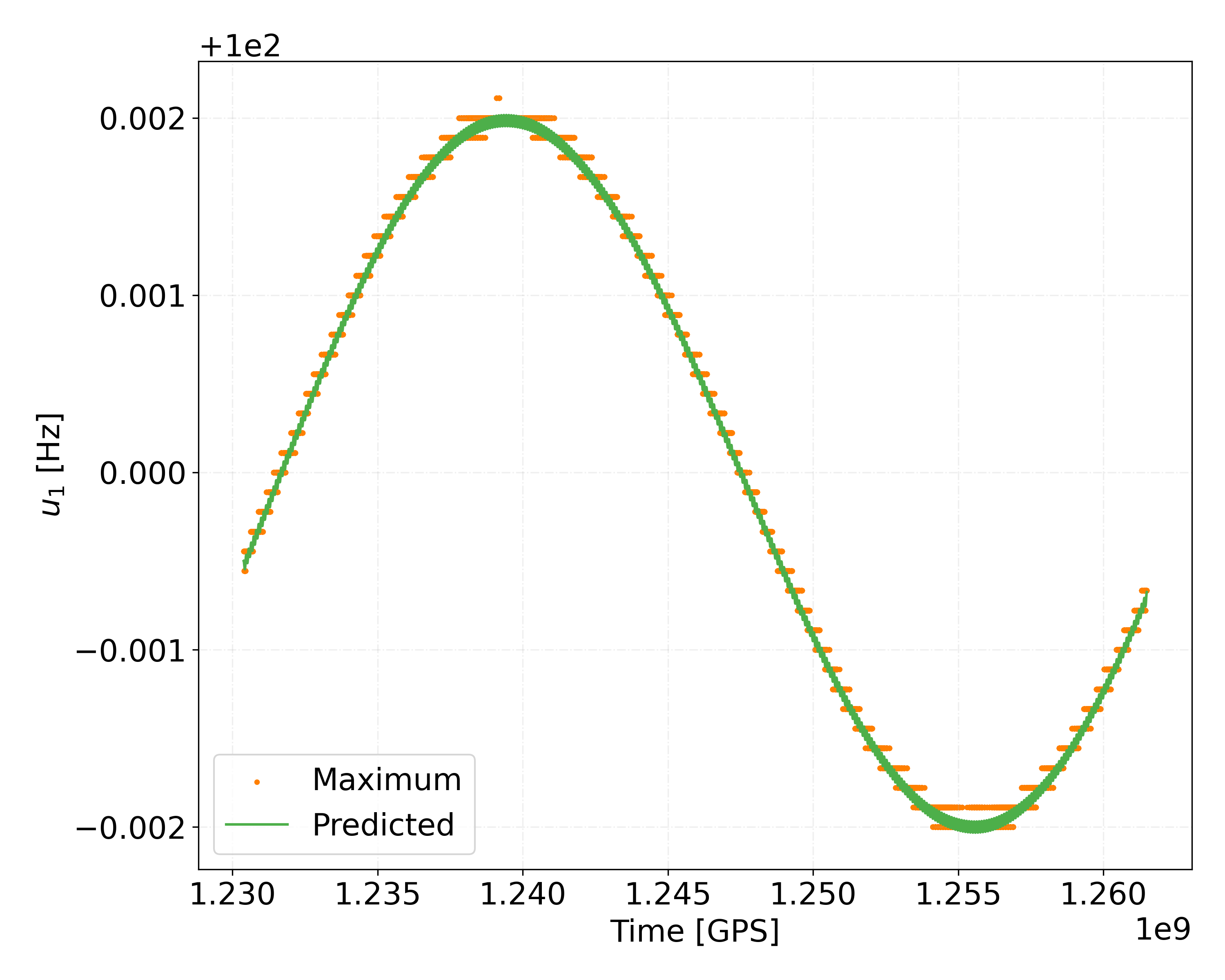
Figure 1: Comparison between the $u_{\mathrm{I}1}$ coordinate per segment given by Eq. (25) (green line) and the $u_{1}$ values per segment that maximize the signal power (orange points). The sky position is offset by $0.3\text{\,}\mathrm{r}\mathrm{a}\mathrm{d}$ in both $\alpha$ and $\delta$ from the signal. This example assumes a single detector (H1) and one year of data, with segments of length $T_{\mathrm{seg}}=$900\text{\,}\mathrm{s}$$, and a constant-frequency signal of $f_{0}=$100\text{\,}\mathrm{H}\mathrm{z}$$ without binary modulation.

The parameter-space bounds for each of the Taylor coordinates are found using Eqs. (25) and (26), by calculating the maximum possible values over the given physical parameter space.

For computational efficiency reasons (namely the look-up table approach used here, see [16]) the first-stage “Hough” semi-coherent summation actually uses the following approximate expressions instead of Eqs. (25) and (26), namely

$$u_{\mathrm{IH}1} =f_{\mathrm{m}}(1-R^{\prime}_{\mathrm{m}})+f_{\mathrm{H}}\,\vec{v}_{\mathrm{m}}\cdot\delta\hat{n},$$ (27)

$$u_{\mathrm{IH}2} =u_{2},$$ (28)

with the “middle” frequency $f_{\mathrm{H}}$ given by

$$f_{\mathrm{H}}\equiv f_{0\mathrm{H}}+f_{1\mathrm{H}}(t_{\mathrm{mid}}-\tau_{\mathrm{ref}})+\ldots,$$ (29)

where the $f_{k\mathrm{H}}$ denote the midpoints in frequency- and spindown-ranges currently being searched over, and $t_{\mathrm{mid}}$ is the mid-time of the full dataset.

III.3 Mismatch

In this subsection we describe and characterize different sources of mismatch for the BinarySkyHou$\mathcal{F}$ pipeline. The mismatch is defined as the relative loss of signal power, namely

$$\mu=1-\frac{\rho_{\mathrm{r}}^{2}}{\rho^{2}},$$ (30)

where $\rho^{2}$ is the full signal power (given by Eq. 20 in [11]) and $\rho_{\mathrm{r}}^{2}$ is the signal power recovered by the search.

The total mismatch of the BinarySkyHou$\mathcal{F}$ pipeline has several contributions, which can be separated in coherent and semi-coherent mismatches. The main contributions to the coherent mismatch are offsets between signal and the closest template in the coherent template grid, and the usage of the (truncated) Taylor coordinates $u_{k}$, while the semi-coherent mismatch is produced by signal-template offsets in the semi-coherent grid and approximations in the interpolation mapping (discussed in the previous section).

III.3.1 Mismatch due to Taylor-coordinate truncation

The usage of a limited number of Taylor coordinates $u_{k}$ incurs an intrinsic mismatch due to the corresponding approximation of the signal waveform. In practice we currently envisage using only $u_{1}$ or at most up to order $u_{2}$, which turns out to be sufficient for currently considered practical all-sky binary searches (similar to the recent search [1] using only $u_{1}$) due to computational constraints. Therefore we quantify the mismatch and corresponding constraints on the maximum coherent segment length $T_{\mathrm{seg}}$ due to truncation to order $u_{1}$ or $u_{2}$.

The mismatch $\mu_{u_{k}}$ due to omission of order $u_{k}$ (and higher) can be estimated as $\mu_{u_{k}}\sim g_{kk}\,u_{k}^{2}$ using the metric $g_{kl}$ in $u_{k}$-space, which is given in Eqs. (56, 57) of [4]. Using this we can express the mismatch due to truncation of $u_{k\geq 2}$ or $u_{k\geq 3}$ as

$$\mu_{u_{2}} \approx g_{22}\,u_{2}^{2}=\frac{\pi^{2}\,T_{\mathrm{seg}}^{4}}{180}\,u_{2}^{2},$$ (31)

$$\mu_{u_{3}} \approx g_{33}\,u_{3}^{2}=\frac{\pi^{2}\,T_{\mathrm{seg}}^{6}}{4032}\,u_{3}^{2}.$$

Using a time-average $\left\langle.\right\rangle$ over segments together with Eq. (16) for $u_{2}$ we obtain $\left\langle u_{2}^{2}\right\rangle\approx\frac{1}{2}f_{0}^{2}a_{\mathrm{p}}^{2}\Omega^{4}+f_{1}^{2}$ (neglecting smaller corrections), and for $u_{3}$ we can use Eq. (58) of [4] as an estimate, which yields $\left\langle u_{3}^{2}\right\rangle\approx\frac{1}{2}f_{0}^{2}a_{\mathrm{p}}^{2}\,\Omega^{6}$, and so we obtain the (segment-averaged) mismatch estimates as

$$\left\langle\mu_{u_{2}}\right\rangle \approx\frac{\pi^{2}\,T_{\mathrm{seg}}^{4}}{360}\,\left(f_{0}^{2}a_{\mathrm{p}}^{2}\Omega^{4}+2f_{1}^{2}\right),$$ (32)

$$\left\langle\mu_{u_{3}}\right\rangle \approx\frac{\pi^{2}\,T_{\mathrm{seg}}^{6}}{8064}\,f_{0}^{2}a_{\mathrm{p}}^{2}\,\Omega^{6}\,,$$ (33)

which illustrate the fact that the segments must be short compared to the orbital period, i.e., $T_{\mathrm{seg}}\,\Omega\ll 1$, in order for the Taylor-coordinates $u_{k}$ to be a good approximation, as discussed in [4].

We can rearrange these equations to obtain a constraint on the maximum coherent time $T_{\mathrm{seg}}$ allowed for a given acceptable mismatch $\left\langle\mu_{u}\right\rangle$ from Taylor truncation, namely when using only $u_{1}$ we find

$$T_{\mathrm{seg}}{}_{,u_{1}} \leq\left(\frac{360\,\left\langle\mu_{u}\right\rangle}{\pi^{2}\left(f_{0}^{2}a_{\mathrm{p}}^{2}\Omega^{4}+2f_{1}^{2}\right)}\right)^{1/4},$$ (34)

and similarly for truncation after $u_{2}$ we obtain the constraint

$$T_{\mathrm{seg}}{}_{,u_{2}} \leq\left(\frac{8064\,\left\langle\mu_{u}\right\rangle}{\pi^{2}f_{0}^{2}a_{\mathrm{p}}^{2}\Omega^{6}}\right)^{1/6}.$$ (35)

These expressions for the maximum coherent time are illustrated in Fig. 2 as a function of frequency for different choices of binary orbital parameters. It can be seen that when $u_{2}$ is also used the maximum coherent time increases by a certain factor.

Figure 3 shows a test of the mismatch predicted by Eq. (32), by generating $1000$ different signals with a frequency of $300\text{\,}\mathrm{H}\mathrm{z}$ and random orbital parameters log-uniformly distributed, with $\Omega\in[0.1,1]\,$\mathrm{d}\mathrm{a}\mathrm{y}\mathrm{s}$$ and $a_{\mathrm{p}}\in[0.01,1]\,$\mathrm{l}\mathrm{s}$$. For each signal we measure the perfectly-matched signal power when using physical coordinates and compare it to the signal power obtained with Taylor coordinates up to order $u_{1}$. The corresponding measured mismatch is then compared to the model prediction of Eq. (32). The figure shows that these equations correctly predict the measured mismatch, in the range where the metric approximation is expected to be accurate (i.e., below mismatches of $\sim 0.3$).

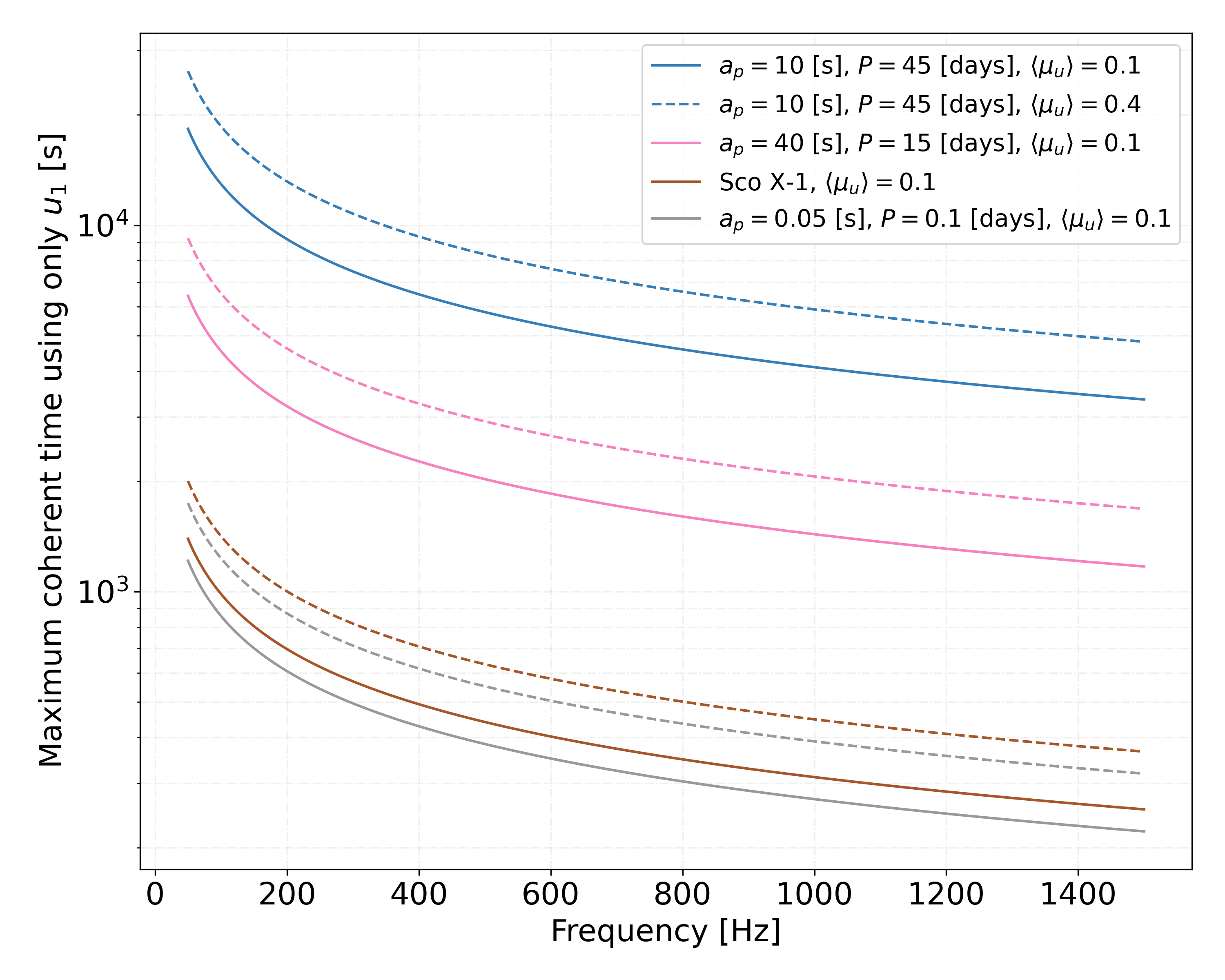
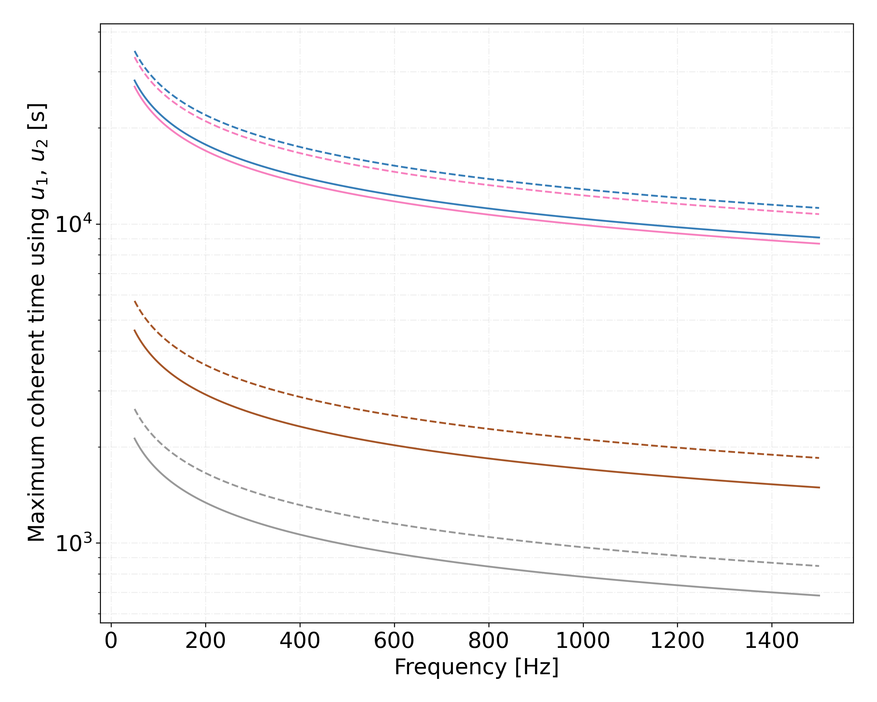
Figure 2: The left plot shows the maximum coherent time $T_{\mathrm{seg}}$ that can be used in a given region of the binary parameter space with a certain mismatch due to the Taylor truncation (assuming zero spindown $f_{1}=0$). The left plot shows the results for $\left\langle mu_{u}\right\rangle=0.1$ (solid lines) and $\left\langle\mu_{u}\right\rangle=0.4$ (dashed lines) in Eq. (34), using only $u_{1}$ Taylor coordinate. The right plot shows the same when using both $u_{1}$ and $u_{2}$ Taylor coordinates.

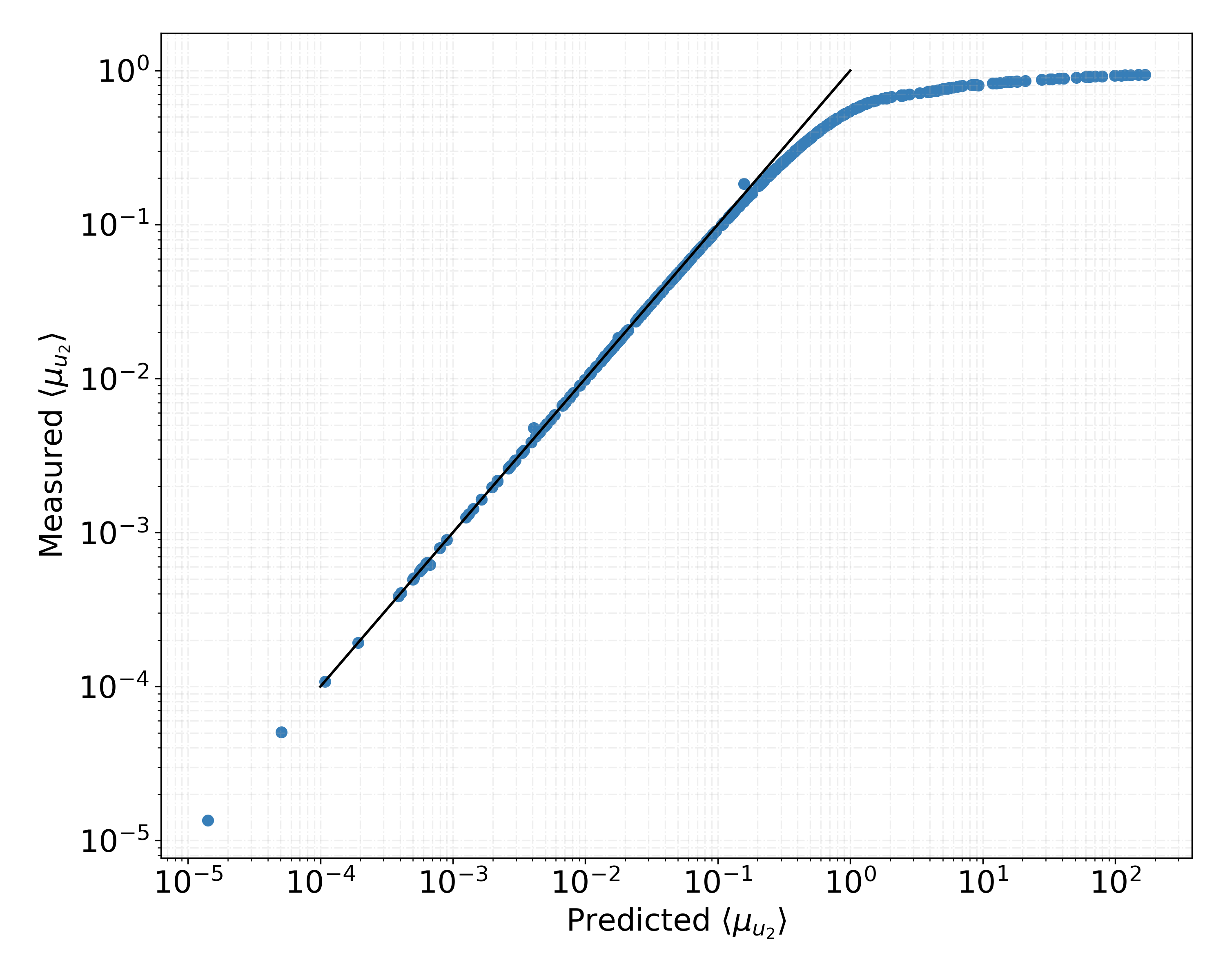
Figure 3: Measured mismatch $\left\langle\mu_{u_{2}}\right\rangle$ (blue points) from Taylor truncation (averaged over segments) against the predicted mismatch (solid line) given by Eq. (32), using $1000$ injections and assuming one year of data from the H1 detector with coherent segments of $T_{\mathrm{seg}}=$900\text{\,}\mathrm{s}$$.

III.3.2 Total mismatch

In the previous subsection we discussed the mismatch contribution due to using a limited set of Taylor coordinates. Additionally there will be template-bank mismatches incurred from the coherent and semi-coherent template grids. If we count the Taylor-truncation mismatch $\mu_{u}$ as part of the coherent mismatch $\mu_{\mathrm{c}}$, then the total average (over the template bank) mismatch $\left\langle\mu\right\rangle$ will be given approximately [7] by the sum of the mean coherent $\left\langle\mu_{\mathrm{c}}\right\rangle$ and mean semi-coherent mismatch $\left\langle\mu_{\mathrm{s}}\right\rangle$, namely

$$\left<\mu\right>\simeq\left\langle\mu_{\mathrm{c}}\right\rangle+\left\langle\mu_{\mathrm{s}}\right\rangle.$$ (36)

From this expression it can be seen that if the mean coherent mismatch is reduced while the semi-coherent mismatch is equal, the total mismatch would decrease.

This is shown in Fig. 4, where the total measured mismatch can be seen for two different cases, which have different $u_{1}$ coherent grids but the same semi-coherent grid (the coherent sky position is the same for both cases, and it is shifted from the signal value). A decrease in the total mismatch can be seen for the case where the coherent $u_{1}$ grid is finer, as predicted by the previous equation. This represents an improvement over the previous pipeline, where the coherent frequency grid was fixed to be equal to the Fourier transform spacing.

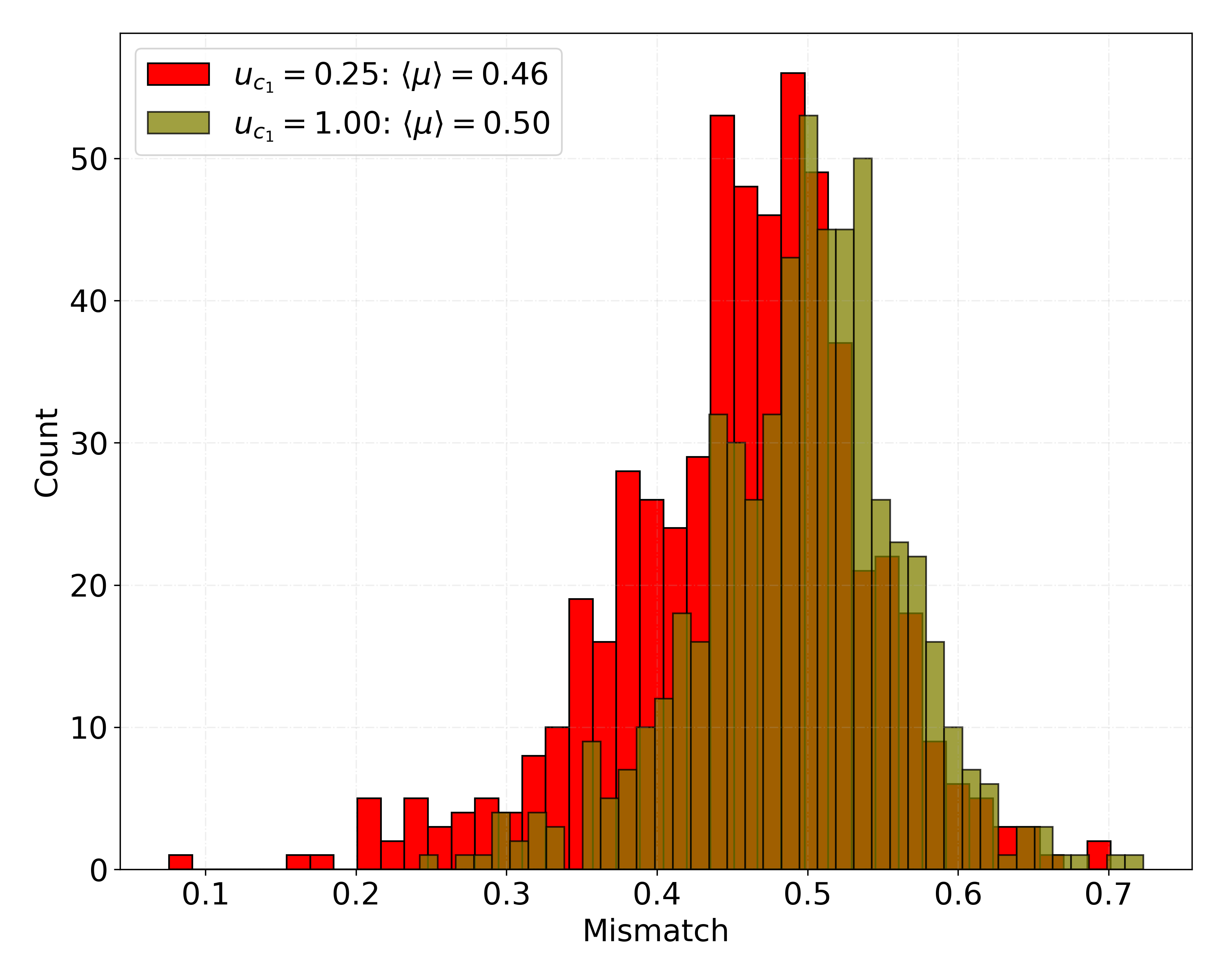
Figure 4: Mismatch histograms for $1000$ injections with random parameters, assuming one year of data from both H1 and L1 detectors and coherent segments of $T_{\mathrm{seg}}=$900\text{\,}\mathrm{s}$$. The olive (right) histogram corresponds to a grid resolution of $\delta u_{1}=1/T_{\mathrm{seg}}$, while the red (left) histogram uses a finer resolution of $\delta u_{1}=0.25/T_{\mathrm{seg}}$. Only $u_{1}$ and a single sky position are searched in the coherent stage. The semi-coherent grids are equal for both cases.

III.3.3 Maximum spindown and eccentricity

Although BinarySkyHou$\mathcal{F}$ is able to search the $f_{1}$ spindown and eccentricity $e$ parameters in the semi-coherent summation, all-sky searches for neutron stars in binary systems are so computationally expensive that one would usually not explicitly search over these parameters at first. For this reason, we want to estimate the value ranges in these omitted parameters to which the pipeline is still sensitive, which will depend on the particular set-up (such as the amount of data and the coherent time).

The maximum covered spindown value $|f_{1}|$ is important for interpreting astrophysical upper limits, since this limits the maximum “mountain height” (NS deformation) or r-mode amplitude that the search can find. The reason for this is that larger deformation (or mode amplitude) would produce a larger spindown $|f_{1}|$ due to the emission of gravitational waves, which would potentially become undetectable by such a search if it was too large.

The semi-coherent grid is constructed by requiring a maximum mismatch $\mu_{\mathrm{M}}$. We can estimate the maximum allowed values by calculating the required resolution for these parameters:

$$|f_{1;\mathrm{max}}|\equiv\delta f_{1} =\sqrt{\frac{\mu_{\mathrm{M}}}{g_{f_{1}f_{1}}}}=\sqrt{\frac{45\mu_{\mathrm{M}}}{4\pi^{2}T_{\mathrm{seg}}^{2}T^{2}_{\mathrm{obs}}}},$$ (37)

$$e_{\mathrm{max}}\equiv\delta e =\sqrt{\frac{\mu_{\mathrm{M}}}{g_{ee}}}=\sqrt{\frac{6\mu_{\mathrm{M}}}{\pi^{2}T_{\mathrm{seg}}^{2}f_{0}^{2}\,\Omega^{2}a_{\mathrm{p}}^{2}}},$$

where $g_{f_{1}f_{1}}$ is obtained from [29] assuming that the refinement factor is equal to $N_{\mathrm{seg}}$ (i.e., there are no gaps), and $g_{ee}$ is found in [4].

It can be seen that for spindown $f_{1}$ the maximum value only depends on the segment length $T_{\mathrm{seg}}$ and total amount of data, while the maximum eccentricity $e$ depends on the frequency $f_{0}$ and orbital parameters $a_{\mathrm{p}}$ and $\Omega$. To obtain a limit, one can take the parameters that produce the most conservative eccentricity, or calculate a mean value over the parameter-space boundaries. The eccentricity equation has the exact same functional form as Eq. (43) in [14], while here we make explicit the dependence on the desired maximum mismatch.

The previous equations quantify the additional mismatch produced by a signal with nonzero spindown $f_{1}$ and eccentricity $e$. However, another potential side-effect would be a shift in the remaining estimated parameters due to correlations between the parameters. However, values exceeding the limits above would not automatically mean such signals are undetectable, only that the resulting mismatch would be larger, thus decreasing the sensitivity of the search.

We can compare the mismatch distribution obtained with the same grid, for four different cases: signals with $f_{1}=0$ and $e=0$; signals with the maximum values; signals with values in between (with log-uniform distributions up to the maximum value); signals with double the maximum value. This is shown in Fig. 5, where it can be seen that signals with parameters at the maximum value (the eccentricity maximum has been calculated using the binary parameters that give the largest eccentricity) increase the mean mismatch by $\sim 0.08$, which would reduce the sensitivity of a search by $\sim 5\%$.

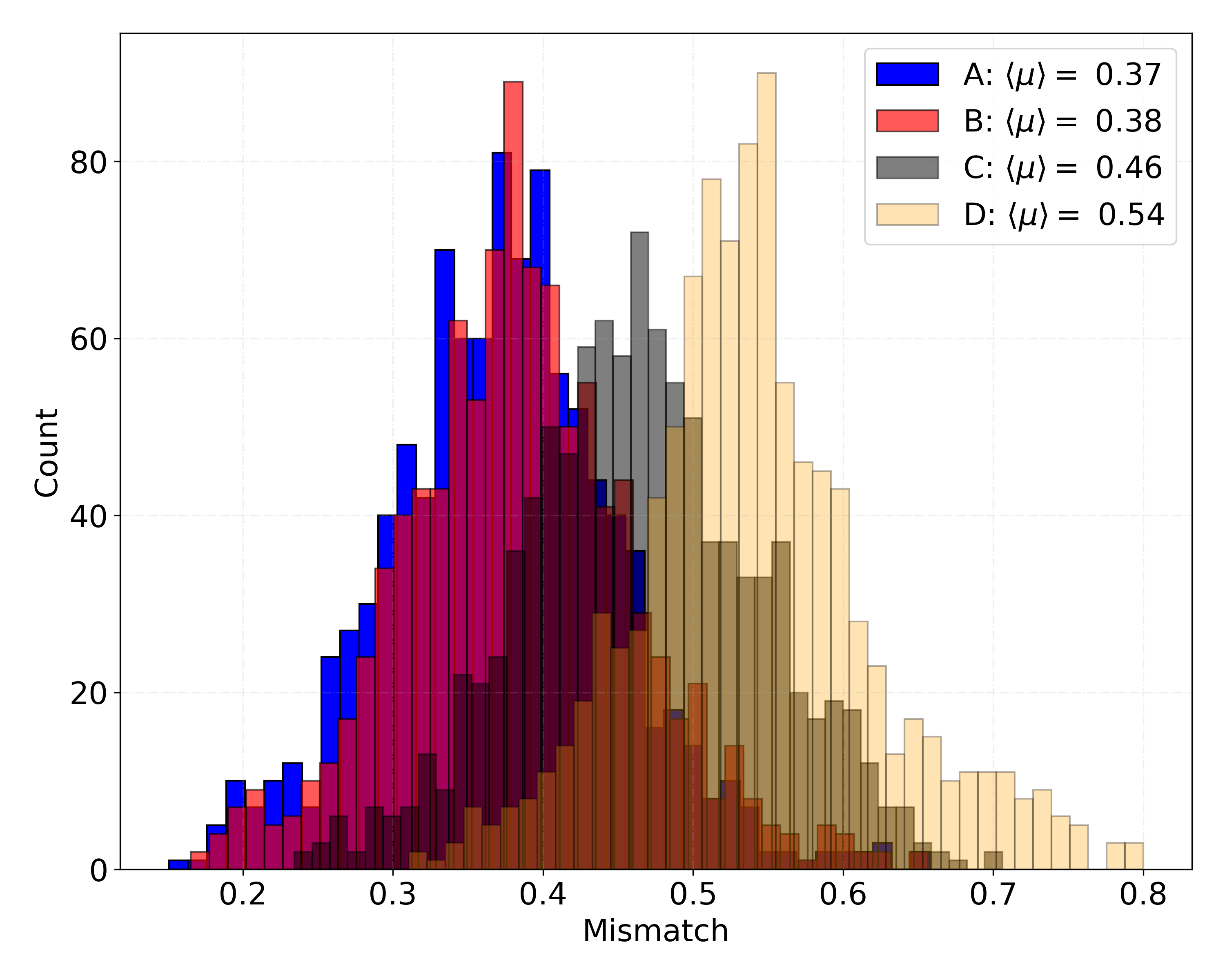
Figure 5: Measured mismatch for $1000$ injections with random parameters, assuming one year of data from the H1 detector and segments of $T_{\mathrm{seg}}=$900\text{\,}\mathrm{s}$$. From left to right, the blue (A) histogram corresponds to signals with zero spindown, $f_{1}=0$, and eccentricity $e=0$; the red (B) histogram uses signals log-uniformly distributed in $f_{1}\in[-4.7\times 10^{-14},-4.7\times 10^{-11}]$ Hz/s and $e\in[0.2\times 10^{-4},0.2\times 10^{-1}]$; the black (C) histogram uses signals with $f_{1}$ and $e$ at their maximum values given by Eq. (37); the yellow (D) histogram is for signals with $f_{1}$ and $e$ given by twice the maximum values.

III.4 Computational model

In this section we explain how the computational cost and Random Access Memory (RAM) of our pipeline scale with different set-up variables, updating and expanding Sec. VF of [14].

III.4.1 Coherent computational cost

Due to the calculation of the $\mathcal{F}$-statistic values, the coherent stage will have an additional computational cost, besides loading the input data and calculating the partial Hough map derivatives. In order to estimate this cost, we summarize the content of [30]. The cost of calculating the $\mathcal{F}$-statistic or its related quantities in segment $\ell$ at a single sky-patch scales with:

$$\tau_{\mathcal{F};\ell} =N_{\mathrm{T;}\ell}\,(N_{u}N_{\mathrm{dterms}}\tau_{\mathrm{core}}+\tau_{\mathrm{buffer}}),$$ (38)

$$N_{\mathrm{T;}\ell} =\sum_{X=1}^{N_{\mathrm{det}}}N_{\mathrm{SFT;}\ell,X},$$ (39)

where $\tau_{\mathrm{core}}$ and $\tau_{\mathrm{buffer}}$ are fundamental timing constants that only depend on the hardware and optimization settings (usually $\tau_{\mathrm{buffer}}$ is approximately one order of magnitude bigger), $2N_{\mathrm{dterms}}+1$ are the number of frequency bins that are used for the calculation of the Dirichlet kernel, $N_{u}$ is the number of coherent $u_{k}$ templates, and $N_{\mathrm{T;}\ell}$ is the total number of SFTs in segment $\ell$.

The total coherent computational cost of a single sky-patch scales with the number of segments:

$$\tau_{\mathcal{F}}=\sum_{\ell=1}^{N_{\mathrm{seg}}}\tau_{\mathcal{F};\ell}=N_{\mathrm{SFT}}(N_{u}N_{\mathrm{dterms}}\tau_{\mathrm{core}}+\tau_{\mathrm{buffer}}).$$ (40)

Since the calculations for each segment are independent from the others, these steps can be easily parallelized. We use an OpenMP loop to take advantage of multi-core CPUs, which can speed-up the calculation by approximately the number of used cores.

The total coherent computational cost will scale linearly with the number of sky-patches.

III.4.2 Semi-coherent computational cost

In the semi-coherent stage the coherent detection statistics are combined for every template that is searched.

The cost of the first stage $\tau_{H;j}$ over a sky-patch $j$ scales as:

$$\tau_{\mathrm{H;}j}=N_{\mathrm{fs}}N_{\mathrm{seg}}\,b(N_{\mathrm{binary}})\,g_{j}(N_{\delta},N_{\alpha},\delta_{u_{1}},\delta_{s})\,h(r)\,\tau_{1},$$ (41)

where $N_{\mathrm{fs}}$ is the number of semi-coherent frequency and spindown templates, $b()$ is a function containing the non-linear dependency on the number of binary templates $N_{\mathrm{binary}}$, $g_{j}()$ is a function describing the effective number of semi-coherent sky points needed (due to the SkyHough algorithm), $N_{\alpha}$ and $N_{\delta}$ are the number of right ascension and declination points in each sky-patch, $\delta_{s}$ is the semi-coherent sky grid resolution, $h()$ is a function that depends on the threshold $r$ set at the coherent stage, and $\tau_{1}$ is a fundamental timing constant. The total semi-coherent cost will scale with the number of sky-patches. In the previous paper [14] it was assumed that $b=N_{\mathrm{binary}}$ and $g_{j}=N_{\delta}N_{\alpha}$, which left some details out.

The function $b()$ depends on the GPU architecture. If we use a CPU, it would simply be equal to $N_{\mathrm{binary}}$, but if we use a GPU it depends non-linearly on parameters such as the occupation of the GPU cores and the usage of shared memory. This can be seen in Fig. 7, where the non-linear scaling with $N_{\mathrm{binary}}$ is clear.

The function $g_{j}()$ is equal or less than $N_{\delta}N_{\alpha}$, and it encodes the SkyHough-type sky interpolation mechanism, which depends on the relation between the size of the annulus produced by the Doppler modulations and the size of the semi-coherent sky grid, as explained in Sec. IVB of [16]. At a given timestamp, the sky-patches with $\hat{n}$ more parallel to $\vec{v}$ have wider annulus, which may contain several semi-coherent sky pixels, thus lowering the number of sky points that need to be taken into account in the semi-coherent loop. This effect will be different at each timestamp, and over a long observing run this will produce an average value between one and $N_{\delta}N_{\alpha}$ for the function $g_{j}()$. This effect gives the SkyHough algorithm a computational advantage.

The function $h$ is different from one for a non-zero threshold $r$, which substitutes coherent values to 0 when below the threshold, thus reducing the computational cost. This function is given by $h=e^{-\frac{r}{\left<r\right>}}$, where $\left<r\right>$ is the expected value of the coherent detection statistic.

We define the average cost $\left\langle\tau_{\mathrm{H}}\right\rangle$ of the first stage over different sky-patches $j$:

$$\left\langle\tau_{\mathrm{H}}\right\rangle=N_{\mathrm{fs}}N_{\mathrm{seg}}\,b(N_{\mathrm{binary}})\left\langle g_{j}(N_{\delta},N_{\alpha},\delta_{u_{1}},\delta_{s})\right\rangle\,h(r)\,\tau_{1}.$$ (42)

The cost $\tau_{\mathrm{R}}$ of the second (i.e., “refinement”) stage scales as:

$$\tau_{\mathrm{R}}=N_{\mathrm{seg}}\,b(N_{\mathrm{cand}})N_{\mathrm{a}}\,\tau_{2},$$ (43)

where $N_{\mathrm{cand}}$ is the number of candidates that are passed to the second stage, $N_{\mathrm{a}}$ is the number of additional points around each candidate that are searched (when using a finer grid), $b()$ is the same function as before, and $\tau_{2}$ is a fundamental timing constant.

The total semi-coherent computational cost is the sum of the first and second stage.

III.4.3 Total computational cost

In order to estimate the total computational cost of a search, we add the coherent and semi-coherent costs (neglecting other costs such as loading the data and writing output to files, since in a realistic scenario they are negligible):

$$\tau=\sum_{l=1}^{N_{\mathrm{F}}}N_{\mathrm{SP;}l}(\tau_{\mathcal{F}}+\left<\tau_{\mathrm{H}}\right>_{l}+\tau_{\mathrm{R;}l}),$$ (44)

where $N_{\mathrm{F}}$ is the number of frequency bands needed to cover a certain frequency range, and $N_{\mathrm{SP;}l}$ is the number of sky-patches at frequency band $l$. The values for $\left<\tau_{\mathrm{H}}\right>_{l}$ and $\tau_{\mathrm{R;}l}$ depend on the frequency band, since $N_{\mathrm{binary}}$, $N_{\delta}$, $N_{\alpha}$, and $N_{\mathrm{cand}}$ scale with frequency.

Figure 6 shows a comparison of the coherent and semi-coherent costs as a function of the number of binary templates. It can be seen that the coherent cost stays constant, but the semi-coherent cost increases, as expected. Past searches using BinarySkyHough and BinarySkyHou$\mathcal{F}$ have used $N_{\mathrm{binary}}$ larger than $10^{5}$, so in such typical scenarios the coherent cost will be a small fraction of the total cost.

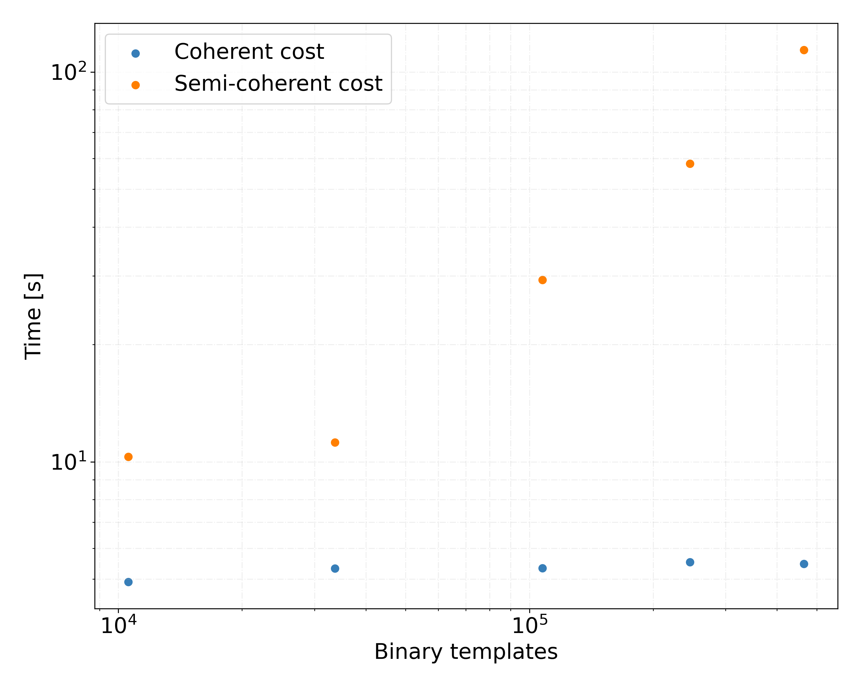
Figure 6: Timing for a single sky-patch of a $0.1\text{\,}\mathrm{H}\mathrm{z}$ frequency band as a function of the number of binary templates. The orange points show the computing time of the semi-coherent stage, while the blue points are for the coherent stage (including the $\mathcal{F}$-statistic computation and generation of partial Hough map derivatives). These timings are obtained on an NVIDIA Tesla V100 and a single core of an Intel(R) Xeon(R) Silver 4215 CPU 2.50 GHz.

If the number of binary templates is small, the coherent computational cost will have a non-negligible impact on the total cost. This also happens for isolated searches, where the search over binary parameters is substituted with a search over $f_{1}$ values, which usually is much less than $10^{5}$. In these two cases, calculating the $\mathcal{F}$-statistic might lower the sensitivity or the span of a search.

When comparing the computational cost to the previous pipeline, it is important to notice that when using the $\mathcal{F}$-statistic as the coherent detection statistic, the total computational cost is reduced compared to using SFT power for multi-detector searches. This is because the semi-coherent summing of the power is done over $\sim N_{\mathrm{seg}}N_{\mathrm{det}}$ values, while the $\mathcal{F}$-statistic generates just $N_{\mathrm{seg}}$ coherent detection statistics. For this reason, in the semi-coherent stage the combination of powers will take roughly $N_{\mathrm{det}}$ times longer than the combination of $\mathcal{F}$-statistic values. If the template grids are the same in both cases, the computational cost of a semi-coherently dominated search using the $\mathcal{F}$-statistic will therefore be reduced. This improvement can be seen in Fig. 7, where the green points show the lowering of the computational cost compared to the orange points.

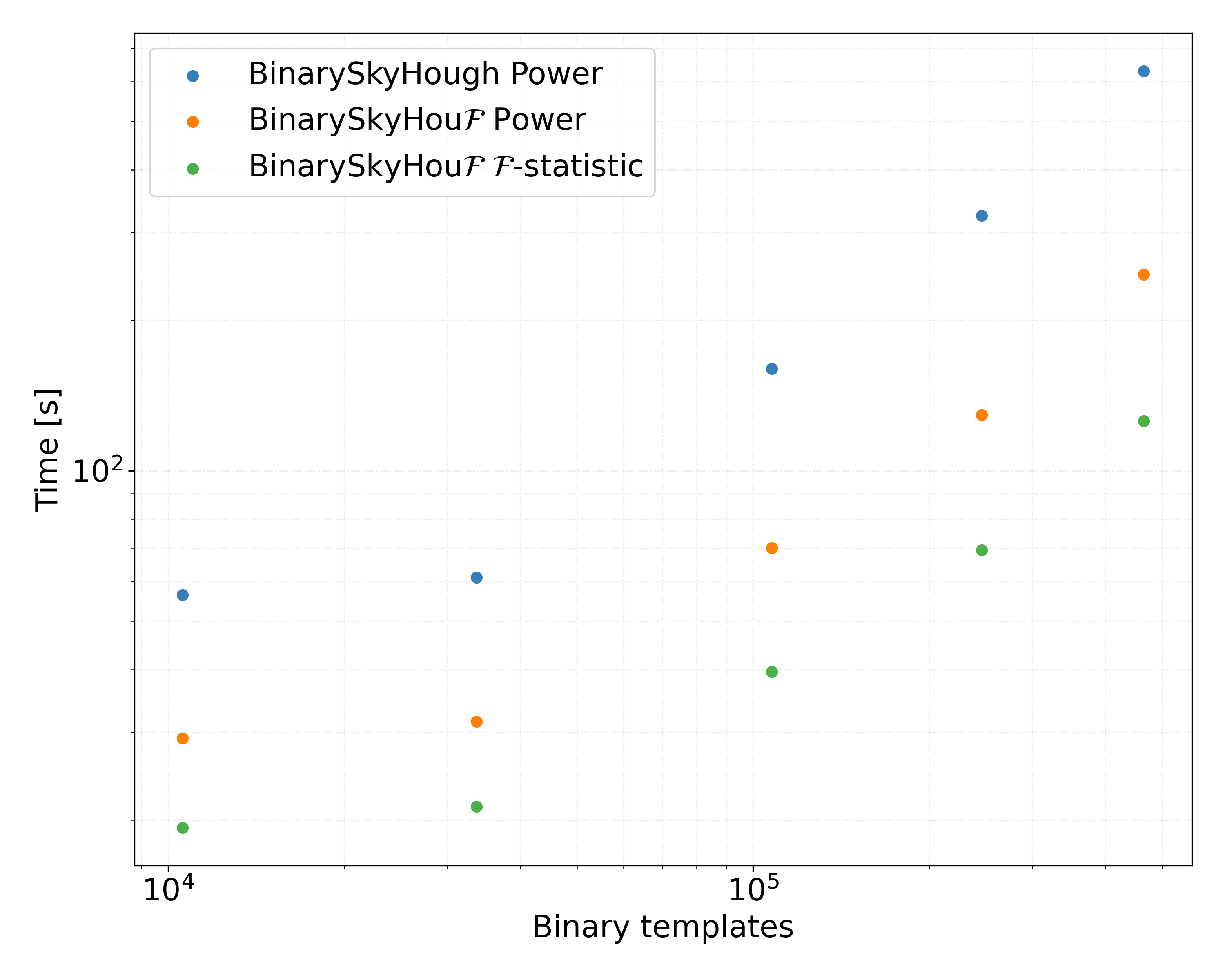
Figure 7: Timing for a single sky-patch of a $0.1\text{\,}\mathrm{H}\mathrm{z}$ frequency band as a function of the number of binary templates. The blue points show the cost of the search for the BinarySkyHough pipeline using SFT power as the coherent detection statistic, the orange points show the cost for the new BinarySkyHou$\mathcal{F}$ pipeline using the power statistic, while the green points refer to using the $\mathcal{F}$-statistic. All three searches use the same number of templates and the same amount of data (Gaussian noise with equal amounts of data from detectors H1 and L1). These timings are obtained on an NVIDIA Tesla V100 and a single core of an Intel(R) Xeon(R) Silver 4215 CPU 2.50 GHz.

Furthermore, the computational efficiency of the code has been improved, mainly by better usage of CUDA’s coalesced global memory access. This can be seen in Fig. 7, comparing the performance of the previous to the new code for the same setup as a function of the number of binary templates (increasing the RAM memory needs). The increased efficiency of the new code corresponds to a lowering of the timing coefficient $\tau_{1}$ in Eq. (41), manifesting as a weaker scaling with the number of binary templates.

III.4.4 RAM

In order to estimate the RAM required by BinarySkyHou$\mathcal{F}$, we find the scaling of the data structures in the code as a function of input parameters such as the maximum mismatch, the coherent time, and the amount of data used.

The biggest data structures in the code are:

• The partial Hough map derivatives, which hold the results from the coherent stage:

  $$S_{\mathrm{P}}=6N_{\mathrm{seg}}N_{u}N_{\mathrm{sky}},$$ (45)

  where $N_{u}$ is the total number of Taylor $u$-coordinate templates, and $N_{\mathrm{sky}}=N_{\delta}N_{\alpha}$ is the number of sky templates.

• The per-frequency bin semi-coherent results:

  $$S_{\mathrm{R}}=8N_{\mathrm{binary}}N_{\mathrm{sky}}.$$ (46)

These structures are orders of magnitude larger than the rest and are therefore enough to give a good estimate of the required RAM.

The main differences with the previous pipeline are:

• The number of frequency bins needed in the partial Hough map derivatives slightly decreases due to the coherent sky demodulation.

• The effective number of “segments” is reduced by the coherent multi-detector combination.

• If more than one Taylor coordinate needs to be used to maintain the mismatch at a certain level, the RAM increases in order to hold the coherent results. This will limit the number of Taylor coordinates that can be used at a certain coherent time.

Another RAM limitation of the code is due to the usage of CUDA’s shared memory in the GPU kernel functions. This limits the size of the sky-patches, which is dependent on the GPU architecture. The shared memory size is given by:

$$S_{\mathrm{S}}=4TN_{\mathrm{sky}},$$ (47)

where $T$ is the number of threads per block in the GPU kernel launch.

IV Sensitivity and parameter estimation

In this section we will estimate the sensitivity of the new pipeline, and compare it to the previous one. In order to do this, we will compare the different detection statistics being used, showing the improvements in sensitivity that are possible due to the usage of demodulated statistics. We are not attempting to estimate a realistic sensitivity that these pipelines would achieve in an actual search, since this also depends on other post-processing procedures, such as clustering or follow-up, which are beyond the scope of the present study.

To estimate the sensitivity, we will follow the same common procedure used in [14]. Namely, for different setups (encompassing the amount of data, detectors and their relative noise levels, maximum mismatch parameters, and coherent time) and detection statistics we generate Gaussian noise and perform a search to obtain the threshold at a certain false alarm probability (in the results shown, we use the top template as the threshold). Next, we add six groups (each with a different gravitational-wave amplitude) of $1000$ randomly distributed signals to the previously generated Gaussian noise, and perform a separate search for each signal. The resulting statistic values are compared to the threshold, and the detection probability is estimated by the fraction of signals detected (i.e., crossing that threshold) out of the total number of signals. This procedure is performed for every different detection statistic.

The injected signals have a random isotropic (NS spin) orientation, a random isotropic sky position, a random frequency $f_{0}$ between $[100,100.1]$ Hz, and a random period $P_{\mathrm{orb}}\in[15,60]$ days and semi-major axis $a_{\mathrm{p}}\in[10,40]$ ls.

The detection statistics that we compare are the original Hough number count (given by Eq. (25) of [14]), the SFT power (given by Eq. (26) of [14]), the $\mathcal{F}$-statistic (given by Eq. (23) of [11]), and the dominant-response statistic (given by Eq. (34) of [11]). For each of these statistics we also compare their weighted versions (discussed in Sec. III.1. Here show the results for a single setup as an illustration, but we have tested various setups with different amounts of data and mismatch distributions and have obtained similar results.

IV.1 Comparison of detection statistics

The left plot of Fig. 8 shows the sensitivity of two unweighted ($\mathcal{F}$ and $\mathcal{F}_{\!{}_{\mathrm{AB}}}$) and three weighted detection statistics (SFT power, $\mathcal{F}$ and $\mathcal{F}_{\!{}_{\mathrm{AB}}}$) for two detectors (H1 and L1), while the right plot shows the same comparison for three detectors (using V1 in addition). In both plots we see that the most sensitive statistic is the weighted dominant-response statistic $\mathcal{F}_{\!{}_{\mathrm{AB}}}$. For the two-detector case, the sensitivities of the SFT power and $\mathcal{F}$-statistic are within the statistical errors of each other, but the right plot shows that for more than two detectors the $\mathcal{F}$-statistic is more sensitive. This is expected from the reduced number of effective segments (as discussed earlier), resulting in reduced $\chi^{2}$ degrees of freedom for the background distribution (e.g., see [11]). We further see that the sensitivity of all statistics improves (on these short segments) when using weights. Overall these results illustrate the sensitivity advantage of the demodulated ($\mathcal{F}$- or $\mathcal{F}_{\!{}_{\mathrm{AB}}}$-) statistics over using SFT power.

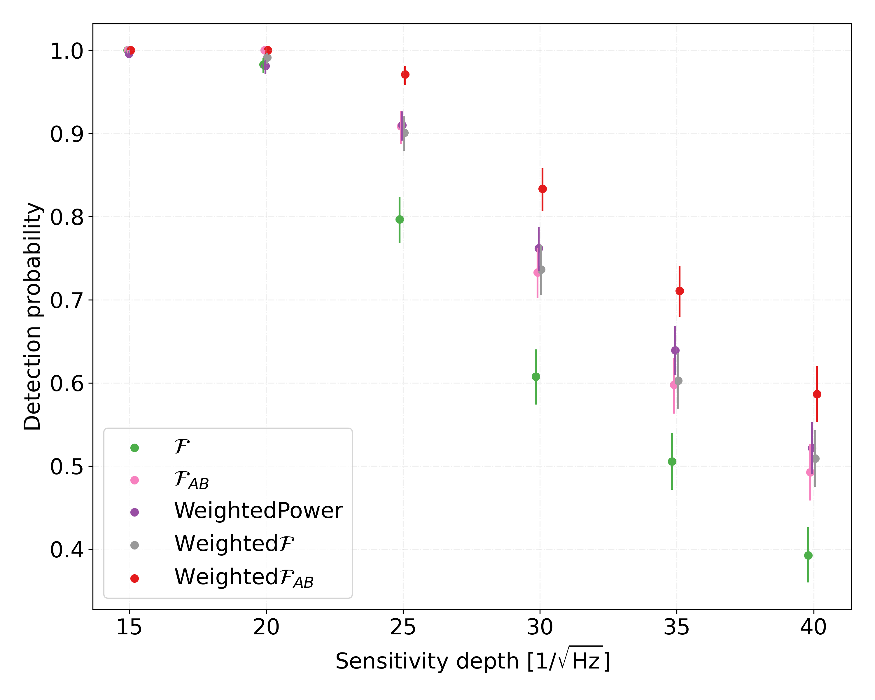
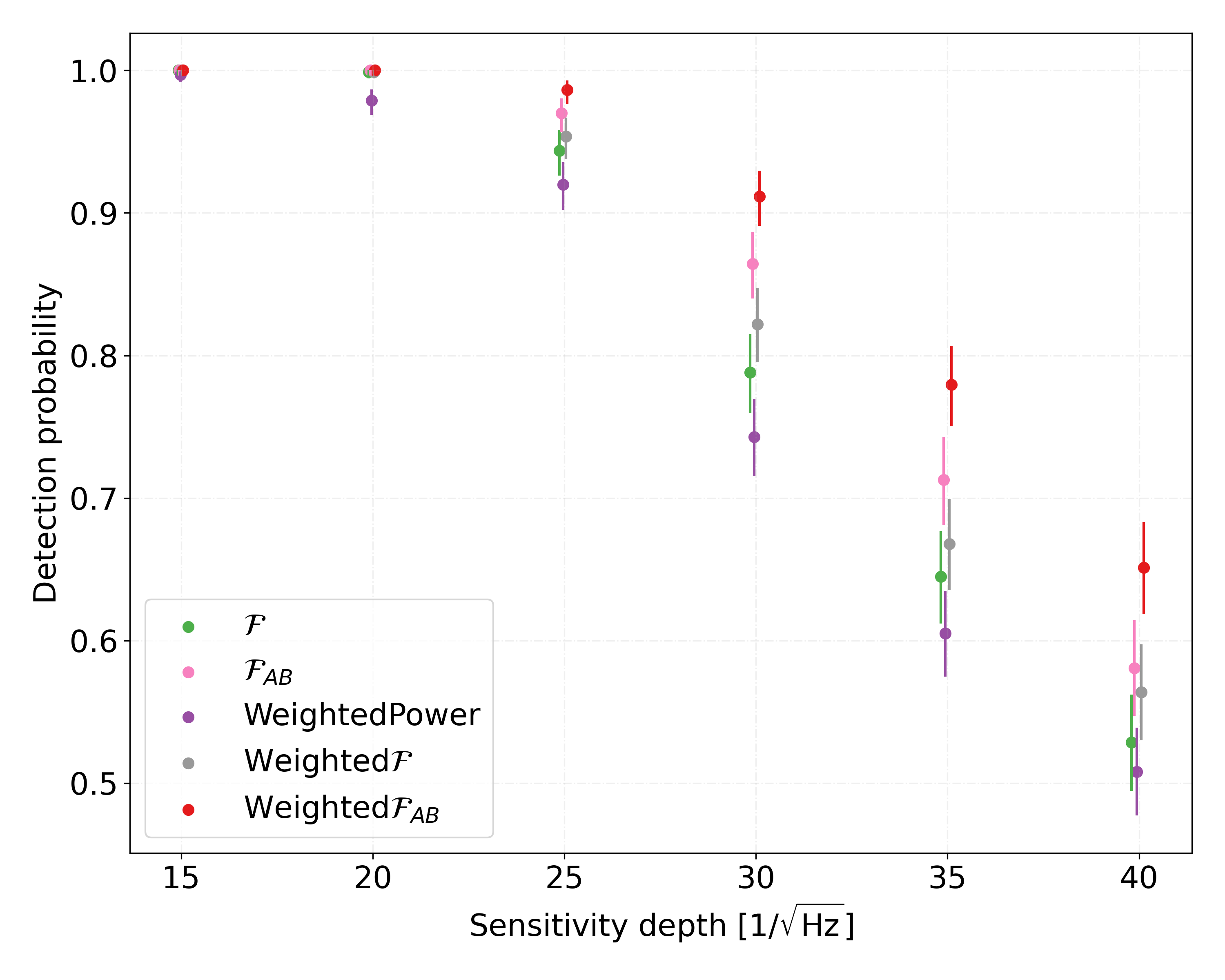
Figure 8: Detection probability as a function of sensitivity depth $\sqrt{S_{\mathrm{n}}}/h_{0}$ for different detection statistics in Gaussian noise. The left plot shows the results for the H1 and L1 detectors, while the right plot additionally includes the V1 detector. The error bars denote the $95\%$ binomial confidence interval. We assume one year of data at the same noise floor from each of the detectors, and a coherent segment length of $T_{\mathrm{seg}}=$900\text{\,}\mathrm{s}$$. (The points have been slightly displaced along the x-axis to ease visibility).

Next we compare the parameter estimation accuracy of the different weighted detection statistics. To do this, we select the template with the highest detection statistic, and compare its parameters with the parameters of the injected signal, if it was detected. The distance between injected signal and recovered “loudest” template is measured in terms of number of grid bins along all six parameter-space dimensions. The results are shown in Fig. 9. It can be seen that the different detection statistics show a very similar behavior, and that for all of them more than $90\%$ of the signals are recovered within one bin.

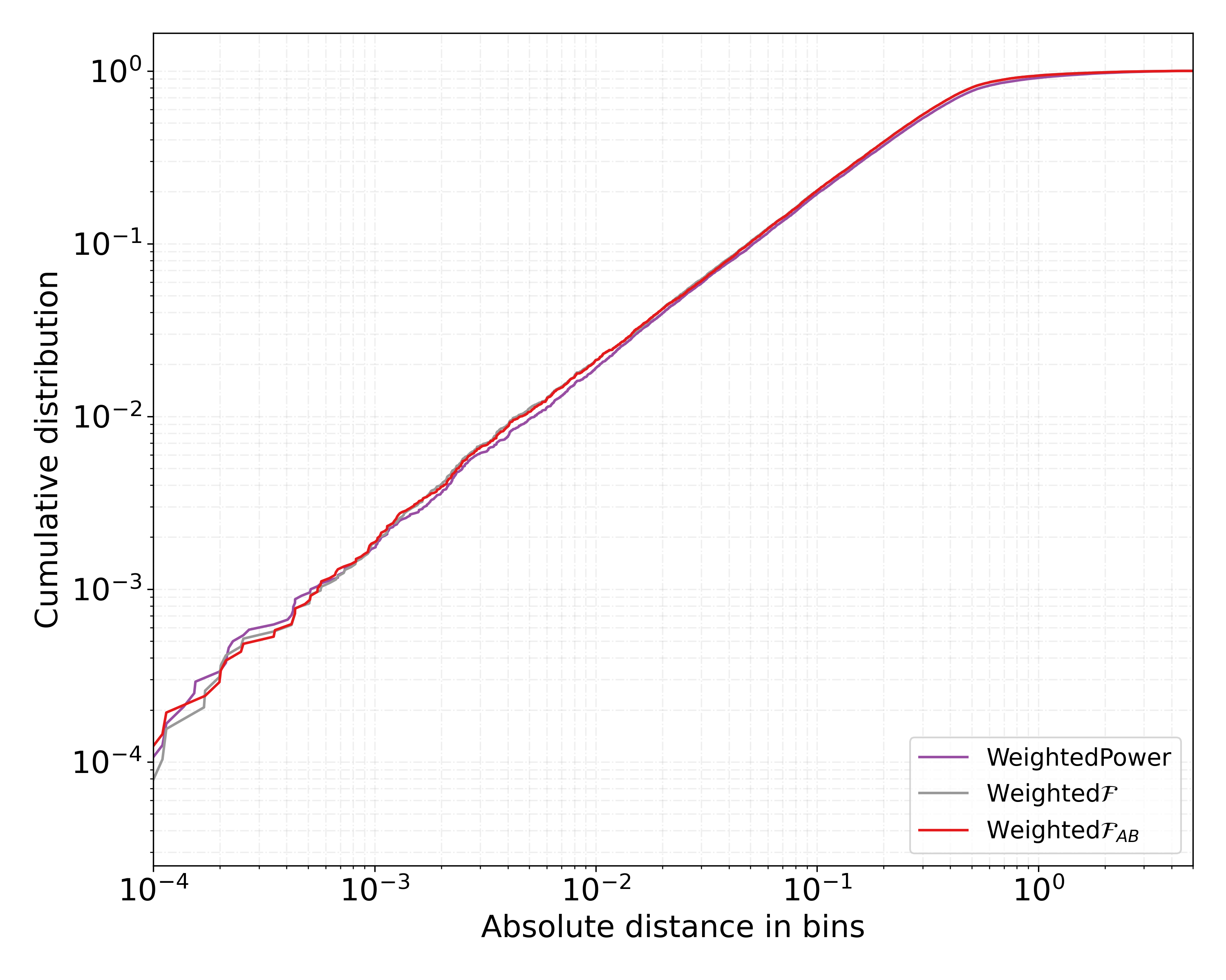
Figure 9: Parameter estimation accuracy for different weighted detection statistics. We plot the cumulative distribution of parameter-space offsets between estimate and injected signal, over the six parameter-space dimensions searched. The plot uses $1000$ injected signals assuming one year of data (with equal Gaussian noise floor) from both the H1 and L1 detectors, and a coherent segment length of $T_{\mathrm{seg}}=$900\text{\,}\mathrm{s}$$.

IV.2 Refinement stage

As discussed in Sec. III.1, the new BinarySkyHou$\mathcal{F}$ pipeline (like the previous BinarySkyHough) consists of two main stages: after the initial search stage, a percentage of templates with the highest detection statistic are reanalyzed with more accurate $u_{\mathrm{I}k}$ interpolation expressions (see Sec. III.2), and possibly with a finer mismatch. The previous BinarySkyHough pipeline also used a more sensitive detection statistic in the second stage, using the weighted power instead of the weighted Hough number count, while now we always use the most sensitive statistic (i.e., weighted $\mathcal{F}_{\!{}_{\mathrm{AB}}}$) in all stages.

The sensitivity of this refinement procedure depends on the percentage of templates that is passed to the second stage. If it is large enough, at a realistically low false alarm probability the sensitivity of the search would be determined by the statistic used in the second stage, thus improving the overall sensitivity. In order to simulate realistic search conditions, for a candidate to count as detected in the second stage we also require its first-stage detection statistic to be higher than the weakest candidate that was passed to the second stage.

Figure 10 shows the comparison of the weighted number count without a second stage with the result when the highest $1\%$ of the candidates are passed to the second stage. We see that the sensitivity of the weighted number count (with the optimal threshold of 3.2) is within the uncertainty errors of the weighted power. This shows that the previous pipeline sensitivity was effectively determined by the second-stage weighted power statistic.

We further see that the sensitivity of the weighted dominant-response $\mathcal{F}_{\!{}_{\mathrm{AB}}}$-statistic is slightly improved in the refinement stage, due to the usage of the more accurate $u_{\mathrm{I}k}$ master equations of Eqs. (25), (26). For more than two detectors, the sensitivities of the demodulated statistics are expected to be even better, similar to what we saw in the right plot of Fig.8.

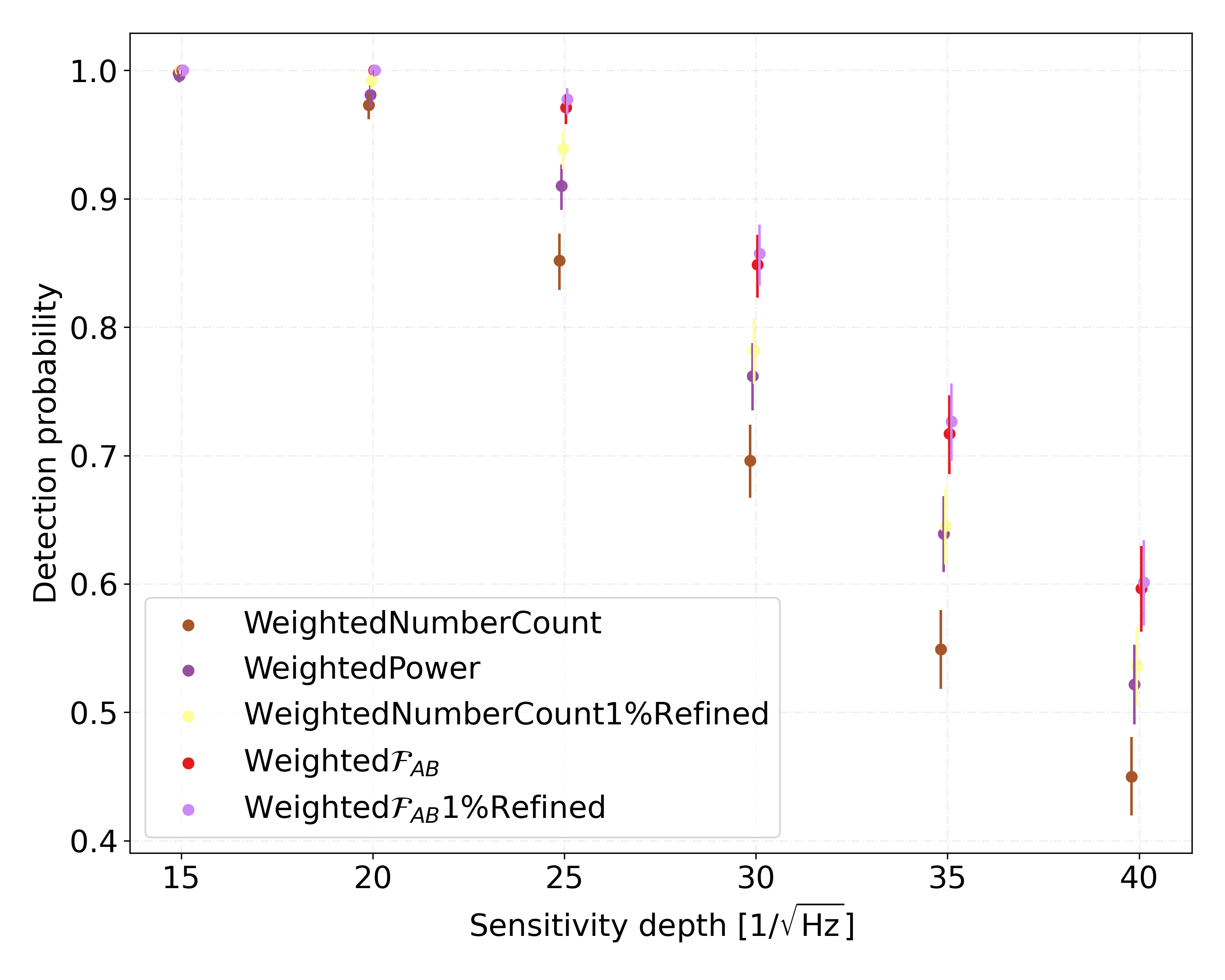
Figure 10: Detection probability as a function of sensitivity depth $\sqrt{S_{\mathrm{n}}}/h_{0}$ for different detection statistics in Gaussian noise. The plot shows the results for the H1 and L1 detectors, assuming one year of data at the same noise floor from each of the detectors, and a coherent segment length of $T_{\mathrm{seg}}=$900\text{\,}\mathrm{s}$$. The error bars denote the $95\%$ binomial confidence interval. (The points have been slightly displaced along the x-axis to ease visibility).

IV.3 Increasing the coherent time

One of the advantages of the new pipeline is the ability to extend the coherent segment time $T_{\mathrm{seg}}$ while maintaining the same mismatch. Using a longer coherent time increases the computational cost, while also increasing the sensitivity of the search. For a large number of segments, the sensitivity of a StackSlide search scales as $N_{\mathrm{seg}}^{-1/4}$ (e.g., [7]), so at fixed false-alarm probability and amount of data, the coherent time would need to be increased by a factor of 16 in order to double the sensitivity of the search.

Here we compare the difference in sensitivity between using a coherent time of $T_{\mathrm{seg}}=$900\text{\,}\mathrm{s}$$ and $T_{\mathrm{seg}}=$3600\text{\,}\mathrm{s}$$, with fixed maximum mismatch parameters.

For this comparison we add random signals from the binary parameter space region of $P_{\mathrm{orb}}\in[0.785,0.8]$ days and $a_{\mathrm{p}}\in[0.5,0.6]$ ls. In this region of the parameter space, several $u_{2}$ templates are needed in order to maintain the same coherent mismatch for the coherent time of $T_{\mathrm{seg}}=$3600\text{\,}\mathrm{s}$$, while the searches with $T_{\mathrm{seg}}=$900\text{\,}\mathrm{s}$$ only need templates in $u_{1}$.

Fig. 11 shows the results by comparing the dominant-response $\mathcal{F}_{\!{}_{\mathrm{AB}}}$-statistic using these two coherent times. The improvement in sensitivity by using a longer coherent time is clear, both for the weighted and unweighted cases. For the unweighted detection statistics, the maximal expected improvement due to the four-times increase in $T_{\mathrm{seg}}$ is around $\sim 1.41$, which agrees approximately with what is seen in the figure.

An interesting point to observe here is that the relative improvement due to weighting of the statistics decreases for longer segment length $T_{\mathrm{seg}}$ (at constant Gaussian-noise floors). This can be understood from the reduced differences in antenna-pattern responses between segments which therefore contribute more similar signal power.

We also show in Fig. 11 a search using the longer $T_{\mathrm{seg}}=$3600\text{\,}\mathrm{s}$$ coherent segments, but without including $u_{2}$ templates. We see that the this decreases its sensitivity, illustrating the need to include $u_{2}$ templates for this setup, as was expected from the mismatch estimates in Sec. III.3.1.

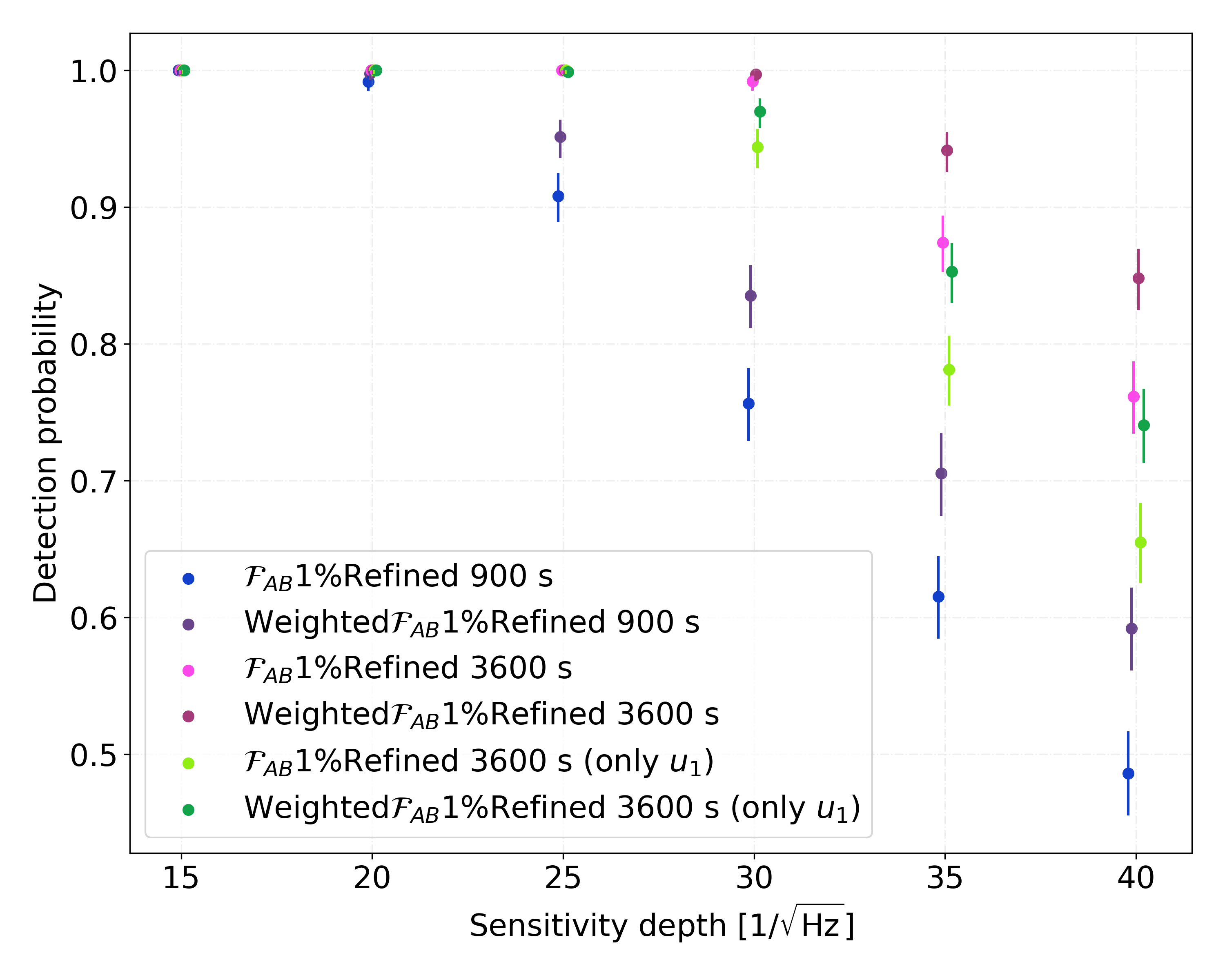
Figure 11: Detection probability as a function of sensitivity depth $\sqrt{S_{\mathrm{n}}}/h_{0}$ for different detection statistics in Gaussian noise, using two different coherent segment lengths, namely $T_{\mathrm{seg}}=$900\text{\,}\mathrm{s}$$ and $T_{\mathrm{seg}}=$3600\text{\,}\mathrm{s}$$. The plot shows the results for the H1 and L1 detectors, assuming one year of data at the same noise floor from each of the detectors. The error bars denote the $95\%$ binomial confidence interval. (The points have been slightly displaced along the x-axis to ease visibility).

V Conclusions

In this paper we have presented a new pipeline, BinarySkyHou$\mathcal{F}$, to search for continuous gravitational waves from unknown neutron stars in binary systems. This new pipeline is a descendant of the previous BinarySkyHough pipeline, improving several different aspects. It can cover the same parameter space at a reduced computational cost, and the usage of demodulated ($\mathcal{F}$- and $\mathcal{F}_{\!{}_{\mathrm{AB}}}$-) statistics allows to use longer coherent segments, which increases sensitivity and gives more flexibility to the pipeline. Furthermore, the per-detector data are combined coherently, thereby reducing the computational cost (by a factor of $\sim N_{\mathrm{det}}$) and further improving sensitivity for searches with more than two detectors.

The new pipeline gives explicit control over the mismatch in the coherent stage, allowing one to perform lower-mismatch searches than before, for example when following up an interesting candidate or targeting a particularly interesting smaller region of parameter space.. One can now explicitly search over binary orbital parameters such as the eccentricity and argument of periapse, or higher-order frequency derivatives. Therefore this pipeline can be used to follow up candidates from different other searches, such as from an all-sky isolated search that only gives constraints on the ranges of possible binary parameters to follow-up.

BinarySkyHou$\mathcal{F}$ also has some limitations. The Taylor coordinates used in the coherent stage only allow searching for orbital periods substantially longer than the coherent segment length, as discussed in Sec. III.3.1. This limits the possibilities to search over the shortest orbital periods with longer coherent times. The corresponding RAM requirements limit the number of Taylor coordinates that can be used, which also limits the maximum coherent time that can be used in certain regions of the parameter space.

However, a number of future improvements to this pipeline can be envisaged. For example, the usage of a non-zero threshold on the coherent statistics before summing, or including only a subset of segments in the first stage depending on their sensitivity. Further enhancements could be achieved by reducing the second-stage mismatch by refining the search grid. It would also be interesting to develop an explicit optimization algorithm for the optimal search setup parameters given a certain amount of data and computational budget, similar to what was done in [7, 31]. We also plan to explore the usage of further demodulated detection statistics, in particular the line-robust statistics of [32], which should help mitigate against non-Gaussian artifacts in the data.

Appendix A Detector-frame Taylor coordinates

In Sec. II we introduced short-segment SSB Taylor coordinates $\{u_{k}\}$, defined by the Taylor expansion of the signal phase in the SSB frame around each segment mid-point. Here we show how similar detector-frame Taylor coordinates $\{u_{k}^{X}\}$ can be expressed for the phase evolution in the frame of detector $X$, which additionally includes the phase modulation due to the detector motion.

In complete analogy to Eq. (10) we can write the Taylor-expansion in detector arrival time $t$ around a mid-time $t_{\mathrm{m}}$:

$$\phi^{X}(t)=\phi_{0}+2\pi\sum_{k=1}^{k_{\max}}\frac{u^{X}_{k}}{k!}\,(t-t_{\mathrm{m}})^{k}\,,$$ (48)

with the detector-frame Taylor coordinates $\{u_{k}^{X}\}_{k=1}^{k_{\max}}$ defined as:

$$u^{X}_{k}\equiv\frac{1}{2\pi}\,\left.\frac{d^{k}\phi^{X}}{dt^{k}}\right|_{t_{\mathrm{m}}}\,,$$ (49)

in terms of the timing relation between source-frame (emission) time $\tau$ and detector-frame (arrival) time $t$, obtained by combining Eqs. (4) and (5):

$$\tau^{X}(t)=\tau(t_{{}_{\mathrm{SSB}}}^{X}(t))=t+\vec{r}^{X}(t)\cdot\hat{n}-R(\tau^{X}).$$ (50)

The expressions Eq. (12) are formally identical, with the SSB derivatives $\tau^{(k)}$ replaced by detector-time derivatives $\tau^{X(k)}\equiv d^{k}\tau^{X}/dt^{k}$, which are found as

$$\dot{\tau}^{X} =\left[1+R^{\prime}\right]^{-1}(1+\dot{\vec{r}}^{X}\cdot\hat{n}),$$ (51)

$$\ddot{\tau}^{X} =\left[1+R^{\prime}\right]^{-1}\left(\ddot{\vec{r}}^{X}\cdot\hat{n}-R^{\prime\prime}\,\dot{\tau}^{X}{}^{2}\right),$$

$$\dddot{\tau}^{X} =\left[1+R^{\prime}\right]^{-1}\left(\dddot{\vec{r}}^{X}\cdot\hat{n}-R^{\prime\prime}\,\dot{\tau}^{X}{}^{3}-3R^{\prime\prime}\,\ddot{\tau}^{X}\dot{\tau}^{X}\right),$$

$$\vdots$$

which generalizes Eq. (14).

We can write the first two orders explicitly as

$$\frac{u^{X}_{1}}{f_{\mathrm{m}}} =\frac{1+\vec{v}_{\mathrm{m}}^{X}\cdot\hat{n}}{1+R^{\prime}_{\mathrm{m}}},$$ (52)

$$u^{X}_{2} =\frac{f_{\mathrm{m}}}{1+R^{\prime}_{\mathrm{m}}}\left(\vec{a}_{\mathrm{m}}^{X}\cdot\hat{n}-R^{\prime\prime}_{\mathrm{m}}\left(\frac{u^{X}_{1}}{f_{\mathrm{m}}}\right)^{2}\right)+f^{\prime}_{\mathrm{m}}\,\left(\frac{u^{X}_{1}}{f_{\mathrm{m}}}\right)^{2},$$

with the definitions of Eqs. (17) and (18) (for small eccentricity and a single spindown), and $\vec{v}^{X}_{\mathrm{m}}\equiv\dot{\vec{r}}^{X}(t_{\mathrm{m}})$, $\vec{a}^{X}_{\mathrm{m}}\equiv\ddot{\vec{r}}^{X}(t_{\mathrm{m}})$ and detector velocity and acceleration at the segment mid-time $t_{\mathrm{m}}$, respectively. Again, these coordinates have units of Hz and $\mathrm{H}\mathrm{z}^{2}$ respectively, but now also depend on the detector $X$ and on the sky position $\hat{n}$ of the signal.

Assuming no spindown $f_{1}=0$, a circular orbit ($e=0$), and a non-relativistic orbital velocity $a_{\mathrm{p}}\Omega\ll 1$, Eq. (52) yields an approximate equation for the frequency-time pattern, namely

$$u_{1}^{X} \approx f_{0}\,(1+\vec{v}^{X}_{\mathrm{m}}\cdot\hat{n})\,(1-a_{\mathrm{p}}\Omega\cos\Psi_{\mathrm{m}})$$ (53)

$$\approx f_{0}+f_{0}\,\vec{v}^{X}_{\mathrm{m}}\cdot\hat{n}-f_{0}\,a_{\mathrm{p}}\Omega\cos\Psi_{\mathrm{m}},$$

which is the same as Eq. (15) of [14], evaluated at segment mid-time $t_{\mathrm{m}}$.

References

- Covas et al. [2022] P. B. Covas, M. A. Papa, R. Prix, and B. J. Owen, Constraints on r-modes and Mountains on Millisecond Neutron Stars in Binary Systems, ApJL 929, L19 (2022).
- Sieniawska and Bejger [2019] M. Sieniawska and M. Bejger, Continuous Gravitational Waves from Neutron Stars: Current Status and Prospects, Universe 5, 217 (2019).
- Riles [2022] K. Riles, Searches for Continuous-Wave Gravitational Radiation (2022), arXiv:2206.06447 [astro-ph].
- Leaci and Prix [2015] P. Leaci and R. Prix, Directed searches for continuous gravitational waves from binary systems: parameter-space metrics and optimal Scorpius X-1 sensitivity, Phys. Rev. D. 91, 102003 (2015).
- Tenorio et al. [2021] R. Tenorio, D. Keitel, and A. M. Sintes, Search Methods for Continuous Gravitational-Wave Signals from Unknown Sources in the Advanced-Detector Era, Universe 7, 474 (2021).
- Brady and Creighton [2000] P. R. Brady and T. Creighton, Searching for periodic sources with LIGO. II. Hierarchical searches, Phys. Rev. D. 61, 082001 (2000).
- Prix and Shaltev [2012] R. Prix and M. Shaltev, Search for Continuous Gravitational Waves: Optimal StackSlide method at fixed computing cost, Phys. Rev. D. 85, 084010 (2012).
- Jaranowski et al. [1998] P. Jaranowski, A. Królak, and B. F. Schutz, Data analysis of gravitational-wave signals from spinning neutron stars: The signal and its detection, Phys. Rev. D. 58, 063001 (1998).
- Cutler and Schutz [2005] C. Cutler and B. F. Schutz, Generalized -statistic: Multiple detectors and multiple gravitational wave pulsars, Phys. Rev. D. 72, 063006 (2005).
- Prix and Krishnan [2009] R. Prix and B. Krishnan, Targeted search for continuous gravitational waves: Bayesian versus maximum-likelihood statistics, Class. Quant. Grav. 26, 204013 (2009).
- Covas and Prix [2022] P. Covas and R. Prix, Improved short-segment detection statistic for continuous gravitational waves, Phys. Rev. D. 105, 124007 (2022).
- Goetz and Riles [2016] E. Goetz and K. Riles, Coherently combining data between detectors for all-sky semi-coherent continuous gravitational wave searches, Class. Quant. Grav. 33, 085007 (2016).
- Goetz and Riles [2011] E. Goetz and K. Riles, An all-sky search algorithm for continuous gravitational waves from spinning neutron stars in binary systems, Class. Quant. Grav. 28, 215006 (2011).
- Covas and Sintes [2019] P. B. Covas and A. M. Sintes, New method to search for continuous gravitational waves from unknown neutron stars in binary systems, Phys. Rev. D. 99, 124019 (2019).
- Aasi et al. [2014] J. Aasi et al. (LIGO Scientific Collaboration; Virgo Collaboration), First all-sky search for continuous gravitational waves from unknown sources in binary systems, Phys. Rev. D. 90, 062010 (2014).
- Krishnan et al. [2004] B. Krishnan, A. M. Sintes, M. A. Papa, B. F. Schutz, S. Frasca, and C. Palomba, Hough transform search for continuous gravitational waves, Phys. Rev. D. 70, 082001 (2004).
- Covas and Sintes [2020] P. Covas and A. M. Sintes, First All-Sky Search for Continuous Gravitational-Wave Signals from Unknown Neutron Stars in Binary Systems Using Advanced LIGO Data, Phys. Rev. Lett. 124, 191102 (2020).
- Abbott et al. [2021] R. Abbott et al., All-sky search in early O3 LIGO data for continuous gravitational-wave signals from unknown neutron stars in binary systems, Phys. Rev. D. 103, 064017 (2021).
- Mendell and Landry [2005] G. Mendell and M. Landry, StackSlide and Hough Search SNR and Statistics, Tech. Rep. LIGO-T05003 (DCC, 2005).
- Manchester et al. [2005] R. N. Manchester, G. B. Hobbs, A. Teoh, and M. Hobbs, The Australia Telescope National Facility Pulsar Catalogue, The Astronomical Journal 129, 1993 (2005).
- Lange et al. [2001] C. Lange, F. Camilo, N. Wex, M. Kramer, D. Backer, A. Lyne, and O. Doroshenko, Precision timing measurements of PSR J1012+5307, MNRAS 326, 274–282 (2001).
- Messenger [2011] C. Messenger, A semi-coherent search strategy for known continuous wave sources in binary systems, Phys. Rev. D. 84, 083003 (2011).
- Nieder et al. [2020] L. Nieder, B. Allen, C. J. Clark, and H. J. Pletsch, Exploiting Orbital Constraints from Optical Data to Detect Binary Gamma-ray Pulsars, ApJ 901, 156 (2020).
- Wikipedia contributors [2022] Wikipedia contributors, Faà di Bruno’s formula — Wikipedia, The Free Encyclopedia (2022), [Online; accessed 24-July-2022].
- Aasi et al. [2013] J. Aasi et al., Einstein@Home all-sky search for periodic gravitational waves in LIGO S5 data, Phys. Rev. D. 87, 042001 (2013).
- Krishnan and Sintes [2007] B. Krishnan and A. M. Sintes, Hough search with improved sensitivity, Tech. Rep. LIGO-T070124 (DCC, 2007).
- Putten et al. [2010] S. v. d. Putten, H. J. Bulten, J. F. J. v. d. Brand, and M. Holtrop, Searching for gravitational waves from pulsars in binary systems: An all-sky search, Journal of Physics: Conference Series 228, 012005 (2010).
- Wette et al. [2018] K. Wette, S. Walsh, R. Prix, and M. A. Papa, Implementing a semicoherent search for continuous gravitational waves using optimally constructed template banks, Phys. Rev. D. 97, 123016 (2018).
- Pletsch [2010] H. J. Pletsch, Parameter-space metric of semicoherent searches for continuous gravitational waves, Phys. Rev. D. 82, 042002 (2010).
- Prix [2017] R. Prix, Characterizing timing and memory-requirements of the -statistic implementations in LALSuite, Tech. Rep. LIGO-T1600531 (DCC, 2017).
- Ming et al. [2018] J. Ming, M. A. Papa, B. Krishnan, R. Prix, C. Beer, S. J. Zhu, H.-B. Eggenstein, O. Bock, and B. Machenschalk, Optimally setting up directed searches for continuous gravitational waves in Advanced LIGO O1 data, Physical Review D 97, 024051 (2018), aDS Bibcode: 2018PhRvD..97b4051M.
- Keitel et al. [2014] D. Keitel, R. Prix, M. A. Papa, P. Leaci, and M. Siddiqi, Search for continuous gravitational waves: Improving robustness versus instrumental artifacts, Phys. Rev. D. 89, 064023 (2014).