Large Deviations Principle for the tagged empirical field of a general interacting gas

Abstract

This paper deals with rare events in a general interacting gas at high temperature, by means of Large Deviations Principles. The main result is an LDP for the tagged empirical field, which features the competition of an energy term and an entropy term. The approach to proving this Large Deviations Principle is to first deduce one for the tagged empirical field of non-interacting particles at high temperature, and upgrade that result to interacting particle systems.

1 Introduction and motivation

Consider $N$ particles in a manifold $M$ that interact via a pair-wise interaction and are confined by an external potential. In this paper, we will only consider the cases $M=\mathbb{R}^{d}$, or $M=\mathbb{T}^{d}$, where $\mathbb{T}^{d}$ is the $d-$dimensional torus of length $T$. We will concentrate on the latter. The case $M=\mathbb{R}^{d}$ will be mentioned only in the introduction, and in the Appendix (section 10).

This is modeled by the Hamiltonian

$$\mathcal{H}_{N}(X_{N})=\sum_{i\neq j}g(x_{i}-x_{j})+N\sum_{i=1}^{N}V(x_{i}),$$ (1)

where $X_{N}\in M^{N},$ with $X_{N}=(x_{1},...x_{N})$, $V:M\to\mathbb{R}$ is the confining potential, and $g:M\to\mathbb{R}$ is the pair-wise interaction.

Consider the Gibbs measure $\mathbf{P}_{N,\beta}$ associated to $\mathcal{H}_{N}:$

$$\mathrm{d}\mathbf{P}_{N,\beta}(X_{N})=\frac{1}{Z_{N,\beta}}\exp\left(-\beta\mathcal{H}_{N}(X_{N})\right)\,\mathrm{d}X_{N},$$ (2)

where $\beta=\beta(N)$ is the inverse temperature, and

$$Z_{N,\beta}=\int_{M^{N}}\exp\left(-\beta\mathcal{H}_{N}(X_{N})\right)\,\mathrm{d}X_{N}$$ (3)

is the partition function. A system governed by (2) will be called a general interacting gas, or particle system.

A very frequent form of the pair-wise interaction $g$ in the setting $M=\mathbb{R}^{d}$ is given by

$$\begin{cases}g(x)=\frac{1}{|x|^{d-2}}\text{ if }d\geq 3\\ g(x)=-\log(|x|)\text{ if }d=1,2\end{cases}$$ (4)

We will refer to this setting as the Coulomb case for $d\geq 2$, and log case for $d=1$. Another frequent form of $g$ in the setting $M=\mathbb{R}^{d}$ is given by

$$g(x)=\frac{1}{|x|^{d-2s}},$$ (5)

with $s\in\left(0,\min\left\{1,\frac{d}{2}\right\}\right)$. We will refer to this setting as the Riesz case.

Coulomb and Riesz gases are a classical field with applications in spherical packing [39, 12, 30], Statistical Mechanics [1, 20, 36, 17, 38], Random Matrix Theory [21, 8, 9, 10, 22, 19, 24], and Mathematical Physics [6, 33], among other fields.

The study of a general interacting gas goes back decades [16, 34, 35], and continues to attract attention [14, 23, 11, 15].

Given that there are $N$ particles in space, and that typically they are confined to a compact set by the potential, the distance between the particles is of order $N^{-\frac{1}{d}}$. This means that the scale $N^{\frac{1}{d}}$ is special and will be called the microscopic scale. We will call the original length scale macroscopic. Any length scale which is between these two will be called mesoscopic.

At a macroscopic scale, the system is well-described by the empirical measure. Given $X_{N}=(x_{1},...x_{N}),$ the empirical measure is defined as

$${\rm emp}_{N}(X_{N}):=\frac{1}{N}\sum_{i=1}^{N}\delta_{x_{i}}.$$ (6)

The behavior of systems governed by (2) can be significantly different depending on the order of magnitude of $\beta$. We will call the regime $\beta=\frac{\theta}{N}$ (with $\theta$ constant) the high-temperature regime. In the regime $\frac{1}{N}\ll\beta$, the empirical measure converges (a.s. under the Gibbs measure) to a measure that typically has compact support, and is characterized by minimizing the mean-field limit of the Hamiltonian. In the high-temperature regime, however, this does not happen. Instead, the empirical measure converges (a.s. under the Gibbs measure) to a measure that is everywhere positive. In the Coulomb or Riesz setting, we will call the regime $\beta=\theta N^{\frac{2s-d}{d}}$ the low temperature regime. The reason for identifying this temperature scaling is that in the low-temperature regime, we observe structure at the microscopic level, whereas at higher temperatures we don’t (see [26]), in the sense that the particles resemble a Poisson process.

At a microscopic scale, the system is well-described by the empirical field, which is defined (given a fixed $x\in M$) as

$$\sum_{i=1}^{N}\delta_{N^{\frac{1}{d}}(x_{i}-x)}.$$ (7)

This object is a positive, discrete measure of mass $N$ on $\mathbb{R}^{d}$. Alternatively, the empirical field may be thought of as an element of $\mathbb{R}^{d\times N}$, defined as $N^{\frac{1}{d}}\theta_{x}X_{N}$, where $\theta_{x}$ denotes the element-wise translation by the vector $x$. This object is often hard to study analytically (even in the non-interacting case), so we may define a less fine observable by averaging the empirical field over a compact subset $\Omega\subset M$:

$$\int_{\Omega}\delta_{\left(N^{\frac{1}{d}}\theta_{x}X_{N}\right)}\,\mathrm{d}x.$$ (8)

This last object is a probability measure on the space of point configurations. A more precise observable, which is still not as precise as the empirical field, is the tagged empirical field. It is given by averaging the empirical field while keeping track of the blow-up point. The tagged empirical field is defined as

$$\int_{\Omega}\delta_{\left(x,N^{\frac{1}{d}}\theta_{x}X_{N}\right)}\,\mathrm{d}x.$$ (9)

The tagged empirical field yields a measure on the cross product of $\Omega$ and the space of point configurations. The first marginal of this measure is the Lebesgue measure on $\Omega$, and the second marginal is the averaged non-tagged empirical field, given by equation (8).

The main goal of this paper is to derive a Large Deviations Principle (LDP) for the tagged empirical field at high temperature ($\beta=\frac{1}{N}$) in the setting of a general interaction. This problem is motivated from several angles:

• It was proved in [23] that the empirical field converges to a Poisson process in the high-temperature regime for a very general class of interactions. A natural question is then to quantify this convergence by means of an LDP. Ideally, this would be quantified by an LDP for the empirical field. Still, as mentioned before, this is a very complicated problem, so we can quantify this convergence with an LDP for the tagged empirical field.

• In, [26] the authors treat the Riesz and Coulomb cases at low temperature ($\beta=\theta N^{\frac{2s-d}{d}}$) . They prove that, in this regime, the tagged empirical field satisfies an LDP in $\mathcal{P}(\mathbb{T}^{d}\times{\rm Config})$ at speed $N$ with rate function

  $$\mathcal{F}(\overline{\mathbf{P}})=\begin{cases}\mathcal{G}(\overline{\mathbf{P}})-\inf_{\overline{\mathbf{P}}^{*}}\mathcal{G}(\overline{\mathbf{P}}^{*})\ \ \ \textrm{if}\ \ \ \overline{\mathbf{P}}\in\mathcal{P}_{s,1}(\mathbb{T}^{d}\times{\rm Config})\\ \infty\ \ \ \ \ \ \ \ \ \ \ \ \ \ \ \ \ \ \ \ \ \ \ \ \ \ \textrm{if}\ \ \ \overline{\mathbf{P}}\in\mathcal{P}_{s,1}(\mathbb{T}^{d}\times{\rm Config})\end{cases}$$ (10)

  with

  $$\mathcal{G}(\overline{\mathbf{P}})=\theta\overline{\mathbb{W}}(\overline{\mathbf{P}},\mu_{V})+\overline{\rm Ent}[\overline{\mathbf{P}}|\overline{\mathbf{\Pi}}^{1}].$$ (11)

  The term $\overline{\mathbb{W}}$ is energy-derived and corresponds to the renormalized energy of point processes, see [26] for an exact definition. The term $\overline{\rm Ent}$ is entropy derived, see Section 5 for an exact definition. A natural question is then to understand the behavior of the system in the limit as $\theta$ tends to $0$. We solve this question for general interactions in the regime $\beta=\frac{1}{N}$, and also for Riesz interactions in the regime $\frac{1}{N}\ll\beta\ll N^{\frac{2s-d}{d}}$. A natural expectation is that the rate function consists of dropping the energy term and keeping only the entropy term. This expectation turns out to be close to correct in the regime $\frac{1}{N}\ll\beta\ll N^{\frac{2s-d}{d}}$ for Riesz interactions, but completely wrong for the regime $\beta=\frac{1}{N}$ and general interactions.

• There has been considerable interest in LDPs for particle systems: [5, 31, 11, 14] derive an LDP for the empirical measure, at various temperature regimes. [26, 25, 3] derive an LDP for the tagged empirical field in the small temperature regimes. However, an LDP for the tagged empirical field outside the small temperature regimes has been absent from the literature. This paper fills this gap.

Remark 1.

Throughout the paper, we will commit the abuse of notation by not distinguishing between a measure and its density.

2 Setting and main definitions

This section will introduce the objects that the main theorem deals with. Most of the section discusses the tagged empirical field and related objects. Starting with this section, and until the Appendix (section 10), we will work exclusively in the case of the torus, i.e. $M=\mathbb{T}^{d}$.

We start with definitions related to energy.

Definition 2.1.

We denote the electric self-interaction of a measure $\mu$ by $\mathcal{E}(\mu)$:

$$\mathcal{E}(\mu)=\int_{\mathbb{T}^{d}\times\mathbb{T}^{d}}g(x-y)\,\mathrm{d}\mu\otimes\mu(x,y).$$ (12)

We denote the mean field limit of $\mathcal{H}_{N},$ by $\mathcal{E}_{V}:$

$$\mathcal{E}_{V}(\mu)=\mathcal{E}(\mu)+\int_{\mathbb{T}^{d}}V\,\mathrm{d}\mu.$$ (13)

We also introduce the thermal energy $\mathcal{E}_{V}^{\theta}:$

$$\mathcal{E}_{V}^{\theta}(\mu)=\mathcal{E}_{V}(\mu)+\frac{1}{\theta}{\rm ent}[\mu],$$ (14)

with

$${\rm ent}[\mu]=\begin{cases}\int_{\mathbb{T}^{d}}\log({\mathrm{d}\mu})\,\mathrm{d}{\mu}\quad\text{ if }\mu\text{ is absolutely continuous w.r.t. Lebesgue measure}\\ \infty\quad\text{ o.w.}\end{cases}$$ (15)

Definition 2.2.

We denote by $\mathcal{P}(\mathbb{T}^{d})$ the set of probability measures on $\mathbb{T}^{d}$.

We denote by $\mu_{\theta}$ the minimizer of $\mathcal{E}_{V}^{\theta}$ in $\mathcal{P}(\mathbb{T}^{d})$:

$$\mu_{\theta}:={\rm argmin}_{\mu\in\mathcal{P}(\mathbb{T}^{d})}\mathcal{E}_{V}^{\theta}(\mu).$$ (16)

We will refer to $\mu_{\theta}$ as the thermal equilibrium measure, see section 5.2 for existence, uniqueness, and basic properties.

We now introduce a few basic operations and sets on the manifold $\mathbb{T}^{d}$.

Definition 2.3.

Throughout this section and throughout the paper, we will use the notation $\theta_{\tau}$ for the translation by $\tau$:

$$\theta_{\tau}(x)=x+\tau.$$ (17)

We will also use the notation $\square_{R}(x)$ for the square of side $R$ and center $x$:

$$\square_{R}(x)=\left[x-\frac{R}{2},x+\frac{R}{2}\right]^{d}.$$ (18)

We will use the notation

$$\square_{R}=\square_{R}(0).$$ (19)

We define the dilation by $\lambda$ as a map from $\mathbb{T}^{d}$ to $\lambda\mathbb{T}^{d}$ (the torus of length $\lambda T$), defined as $x\to\lambda x$.

We now introduce the main object that this paper deals with: the tagged empirical field.

Definition 2.4.

Given a bounded open set $\Omega\subset\mathbb{T}^{d},$ and $X_{N}\in\mathbb{T}^{d\times N}$, we define the tagged empirical field

$$\overline{\mathbf{P}}_{N}(X_{N})=\frac{1}{|\Omega|}\int_{\Omega}\delta_{\left(x,\theta_{N^{\frac{1}{d}}x}\cdot X_{N}^{\prime}\right)}\,\mathrm{d}x,$$ (20)

where $X_{N}^{\prime}=N^{\frac{1}{d}}X_{N}$, $\theta_{\tau}$ denotes the element-wise translation by $\tau$, and $|\Omega|$ denotes the Lebesgue measure of $\Omega$.

Having defined the tagged empirical field, we identify some topological spaces of interest and state a few foundational results. This is needed in order to identify the topology of the LDP.

Definition 2.5.

Given an open set $A\subset\mathbb{T}^{d}$, we define ${\rm Config}(A)$ to be the set of locally finite points configurations on $A$. Equivalently, ${\rm Config}(A)$ can be thought of as the set of non-negative, purely atomic Radon measures on $A$ giving an integer mass to singletons. Given a measurable set $B\subset A$, and $\mathcal{C}\in{\rm Config}(A)$ we denote by $|\mathcal{C}|(B)$ the number of points of $\mathcal{C}$ in $B$.

We denote ${\rm Config}:={\rm Config}(\mathbb{T}^{d})$.

We endow ${\rm Config}$ with the topology induced by the topology of weak convergence of Radon measures.

We define the following distance on ${\rm Config}$:

$$d_{\rm Config}(\mathcal{C}_{1},C_{2})=\sum_{k=1}^{\infty}\frac{1}{2^{k}}\sup_{f\in{\rm Lip}_{1}(\mathbb{T}^{d})}\frac{\int_{\square_{K}}f\,\mathrm{d}\left(\mathcal{C}_{1}-\mathcal{C}_{2}\right)}{|\mathcal{C}_{1}|(\square_{k})+|\mathcal{C}_{2}|(\square_{k})},$$ (21)

where ${\rm Lip}_{1}(\mathbb{T}^{d})$ denotes the set of Lipschitz functions on $\mathbb{T}^{d}$ with Lipschitz constant $1$ and such that ${\rm esssup}\{|f|\}\leq 1$. If $k>T$, we think of $\mathbb{T}^{d}$ as a subset of $\square_{k}$.

The following Lemma establishes some basic properties about ${\rm Config}$.

Lemma 2.6.

• The topological space ${\rm Config}$ is Polish.

• The distance $d_{\rm Config}$ is compatible with the topology induced by the topology of weak convergence of Radon measures.

Proof.

See for example [26], Lemma 2.1. ∎

Definition 2.7.

Given a set $\Omega\subset\mathbb{T}^{d}$, we denote by $\mathcal{P}({\rm Config})$ the set of probability measures on ${\rm Config}$, and by $\mathcal{P}(\Omega\times{\rm Config})$ the set of probability measures on $\Omega\times{\rm Config}$. An element of $\mathcal{P}(\Omega\times{\rm Config})$ will be called a tagged point process. We endow $\mathcal{P}(\Omega\times{\rm Config})$ with the distance

$$d_{\mathcal{P}(\Omega\times{\rm Config})}(\overline{\mathbf{P}}_{1},\overline{\mathbf{P}}_{2})=\sup_{F\in{\rm Lip}_{1}(\Omega\times{\rm Config})}\int F\,\mathrm{d}(\overline{\mathbf{P}}_{1}-\overline{\mathbf{P}}_{2}),$$ (22)

where ${\rm Lip}_{1}(\Omega\times{\rm Config})$ denotes the space of Lipschitz functions on the space $(\Omega\times{\rm Config})$ with Lipschitz constant $1$ and such that ${\rm esssup}\{|F|\}\leq 1$. The distance (22) metrizes the topology of weak convergence on $\mathcal{P}(\Omega\times{\rm Config})$ (see [26]).

Now that we have defined the object that the main theorem deals with, and that we have defined a topology on the subspace in which it lives, we turn to define important quantities associated with tagged empirical fields. These are necessary for defining the rate function, and the space on which the LDP is proved.

Definition 2.8.

Given $\overline{\mathbf{P}}\in\mathcal{P}(\Omega\times{\rm Config})$, we define the disintegration measure $\overline{\mathbf{P}}^{x}$, which for each $x\in\Omega$ is an element of $\mathcal{P}({\rm Config})$, characterized by the requirement that for any $F\in C^{0}(\Omega\times{\rm Config})$ we have

$$\mathbf{E}_{\overline{\mathbf{P}}}[F]=\frac{1}{|\Omega|}\int_{\Omega}\mathbf{E}_{\overline{\mathbf{P}}^{x}}[F(x,\cdot)]\,\mathrm{d}x.$$ (23)

See [2] for the existence and uniqueness of the disintegration measure.

Definition 2.9.

Given an open subset $A\subset\mathbb{T}^{d}$, we define the Poisson Point Process of intensity $\lambda$ on $A$ as $\mathbf{\Pi}^{\lambda}\in\mathcal{P}({\rm Config}(A))$ characterized by the requirement that for any Borel set $B\subset A$,

$$\mathbf{\Pi}^{\lambda}\left\{|C|(B)=n\right\}=\frac{(\lambda|B|)^{n}}{n!}\exp\left(-\lambda|B|\right).$$ (24)

Definition 2.10.

Given a set $\Omega\subset\mathbb{T}^{d}$ and a function $\lambda:\Omega\to\mathbb{R}^{+}$, we define the tagged Poisson Point Process $\overline{\mathbf{\Pi}}^{\lambda}\in\mathcal{P}(\Omega\times{\rm Config})$ as the unique tagged point process such that the disintegration measure satisfies that for each $x\in\Omega$,

$$(\overline{\mathbf{\Pi}}^{\lambda})^{x}=\mathbf{\Pi}^{\lambda(x)}.$$ (25)

Definition 2.11.

A point process ${\mathbf{P}}\in\mathcal{P}({\rm Config})$ is called stationary if for any set $A\subset{\rm Config}$ and any vector $\tau\in\mathbb{T}^{d}$,

$$\mathbf{P}(A)=\mathbf{P}(\theta_{\tau}A).$$ (26)

The set of stationary point processes is denoted by $\mathcal{P}_{s}({\rm Config})$.

A tagged point process $\overline{\mathbf{P}}\in\mathcal{P}(\Omega\times{\rm Config})$ is called stationary if $\overline{\mathbf{P}}^{x}$ is stationary for all $x\in\Omega$.

Definition 2.12.

We define the intensity of a point process ${\mathbf{P}}\in\mathcal{P}({\rm Config})$ as

$${\rm int}[\mathbf{P}]:=\mathbf{E}_{\mathbf{P}}[|C|\square_{1}].$$ (27)

Note that, according to this definition, the “Poisson process of intensity $\lambda$” has intensity $\lambda$. Note also that if $\mathbf{P}$ is stationary, then the intensity is equal to

$$\frac{1}{k^{d}}\mathbf{E}_{\mathbf{P}}[|C|\square_{k}]$$ (28)

for any $k>0$.

Definition 2.13.

We say that a tagged point process $\overline{\mathbf{P}}\in\mathcal{P}(\Omega\times{\rm Config})$ has intensity $1$ if

$$\int_{\Omega}{\rm int}[\overline{\mathbf{P}}^{x}]\,\mathrm{d}x=1.$$ (29)

The set of stationary tagged point processes of intensity $1$ is denoted by $\mathcal{P}_{s,1}(\Omega\times{\rm Config})$.

Definition 2.14.

Given two point processes on a compact set $\Omega$, $\mathbf{P}_{1},\mathbf{P}_{2}\in\mathcal{P}({\rm Config}(\Omega))$, we define the relative entropy of $\mathbf{P}_{1}$ with respect to $\mathbf{P}_{2}$ as

$${\rm Ent}[\mathbf{P}_{1}|\mathbf{P}_{2}]=\begin{cases}\int\frac{\mathrm{d}\mathbf{P}_{1}}{\mathrm{d}\mathbf{P}_{2}}\log\left(\frac{\mathrm{d}\mathbf{P}_{1}}{\mathrm{d}\mathbf{P}_{2}}\right)\,\mathrm{d}\mathbf{P}_{2}\ {\rm if}\ \mathbf{P}_{1}\ll\mathbf{P}_{2}\\ \infty\ {\rm o.w,}\end{cases}$$ (30)

where $\frac{d\mathbf{P}_{1}}{d\mathbf{P}_{2}}$ is the Radon–Nikodym derivative.

Given a stationary point process $\mathbf{P}\in\mathcal{P}_{s}({\rm Config})$, and $\lambda>0$ we define the specific relative entropy of $\mathbf{P}_{1}$ with respect to $\mathbf{\Pi}^{\lambda}$ as

$${\rm Ent}[\mathbf{P}|\mathbf{\Pi}^{\lambda}]=\lim_{R\to\infty}\frac{1}{R^{d}}{\rm Ent}[\mathbf{P}|_{\square_{R}}|\mathbf{\Pi}^{\lambda}|_{\square_{R}}],$$ (31)

where $\mathbf{\Pi}^{\lambda}|_{\square_{R}}$ and $\mathbf{P}|_{\square_{R}}$ denote the restrictions of $\mathbf{\Pi}^{\lambda}$ and $\mathbf{P}$ to the set $\square_{R}$, respectively .

Given a tagged point processes $\overline{\mathbf{P}}\in\mathcal{P}_{s}(\Omega\times{\rm Config})$, and a function $\lambda:\Omega\to\mathbb{R}^{+}$, we define the specific relative entropy of $\overline{\mathbf{P}}$ with respect to $\overline{\mathbf{\Pi}}^{\lambda}$ as

$$\overline{\rm Ent}[\overline{\mathbf{P}}|\overline{\mathbf{\Pi}}^{\lambda}]=\int_{\Omega}{\rm Ent}[\overline{\mathbf{P}}^{x}|\mathbf{\Pi}^{\lambda(x)}]\,\mathrm{d}x.$$ (32)

Note that the specific relative entropy with respect to $\overline{\mathbf{\Pi}}^{\lambda}$ is not a function of the disintegration measure alone, since it depends on the configuration of points well as their density.

The following lemma is classical (see, for example, [26]) and establishes some basic properties about the entropy functional.

Lemma 2.15.

For any $\lambda>0$, there holds:

• The limit in equation (31) exists if ${\mathbf{P}}$ is stationary.

• The map $\mathbf{P}\mapsto{\rm Ent}[\mathbf{P}|\mathbf{\Pi}^{\lambda}]$ is affine and lower semi-continuous on $\mathcal{P}_{s}({\rm Config})$.

• The sub-level sets of ${\rm Ent}[\cdot|\mathbf{\Pi}^{\lambda}]$ are compact in $\mathcal{P}_{s}({\rm Config})$ (it is a good rate function).

• We have ${\rm Ent}[\mathbf{P}|\mathbf{\Pi}^{\lambda}]\geq 0$, and it vanishes only if $\mathbf{P}=\mathbf{\Pi}^{\lambda}$.

Lastly, we recall the definitions of rate functions and of Large Deviations Principle.

Definition 2.16 (Rate function).

Let $X$ be a metric space (or a topological space). A rate function is an l.s.c. function $I:X\to[0,\infty]$, it is called a good rate function if its sublevel sets are compact.

Definition 2.17 (LDP).

Let $P_{N}$ be a sequence of Borel probability measures on $X$ and $a_{N}$ a sequence of positive reals such that $a_{N}\to\infty.$ Let $I$ be a good rate function on $X.$ The sequence $P_{N}$ is said to satisfy a Large Deviations Principle (LDP) at speed $a_{N}$ with (good) rate function $I$ if for every Borel set $E\subset X$ the following inequalities hold:

$$-\inf_{E^{\mathrm{o}}}I\leq\liminf_{N\to\infty}\frac{1}{a_{N}}\log\left(P_{N}(E)\right)\leq\limsup_{N\to\infty}\frac{1}{a_{N}}\log\left(P_{N}(E)\right)\leq-\inf_{\overline{E}}I,$$ (33)

where $E^{\mathrm{o}}$ and $\overline{E}$ denote respectively the interior and the closure of a set $E.$ Formally, this means that $P_{N}(E)\simeq\exp(-a_{N}\inf_{{E}}I).$

We have now defined all objects needed for the statement of the main theorem, which we now introduce.

3 Main results

The main result of this paper is the following theorem:

Theorem 3.1.

Assume that $\beta=\frac{\theta}{N}$ and $g:\mathbb{T}^{d}\to\mathbb{R}$ satisfies:

• Symmetry.

  $$g(x)=g(-x).$$ (34)

• Integrability.

  $$g\in L^{1}(\mathbb{T}^{d}).$$ (35)

• Uniform continuity. For any $\epsilon>0,$ we have that $g$ is uniformly continuous on $\mathbb{T}^{d}\setminus B(0,\epsilon)$.

• Weak positive definiteness. If $\mu\in TV(\mathbb{T}^{d})$ is such that

  $$\int_{\mathbb{T}^{d}}\,\mathrm{d}\mu=0,$$ (36)

  then

  $$\mathcal{E}(\mu)\geq 0,$$ (37)

  where $TV(\mathbb{T}^{d})$ denotes the space of signed measures of bounded variation.

• For any $\mu\in\mathcal{P}(\mathbb{T}^{d})$,

  $$\mathcal{E}(\mu)>-\infty.$$ (38)

Assume that the confining potential $V$ satisfies:

• $V$ is lower-semi-continuous.

• $V\in L^{1}(\mathbb{T}^{d})$.

Define $\overline{\mathbf{P}}_{N}$ by Definition 2.4 with $\Omega=\mathbb{T}^{d}$ and $\mu_{\theta}$ by (16). Then the pushforward of the Gibbs measure $\mathbf{P}_{N,\beta}$ (equation (2)) by $\overline{\mathbf{P}}_{N}$ satisfies an LDP in $\mathcal{P}(\mathbb{T}^{d}\times{\rm Config})$ at speed $N$ with rate function

$$\mathcal{F}(\overline{\mathbf{P}})=\begin{cases}\theta\mathcal{E}(\rho-\mu_{\theta})+\overline{{\rm Ent}}[\overline{\mathbf{P}}|\overline{\mathbf{\Pi}}^{\mu_{\theta}}]\ \ \ \textrm{if}\ \ \ \overline{\mathbf{P}}\in\mathcal{P}_{s,1}(\mathbb{T}^{d}\times{\rm Config}),\\ \infty\ \ \ \ \ \ \ \ \ \ \ \ \ \ \ \ \ \ \ \ \ \ \ \ \ \ \ \ \ \ \ \textrm{if}\ \ \ \overline{\mathbf{P}}\notin\mathcal{P}_{s,1}(\mathbb{T}^{d}\times{\rm Config}),\end{cases}$$ (39)

where $\rho$ is the probability measure with density ${\rm int}[\overline{\mathbf{P}}^{x}]$.

The way to prove Theorem 3.1 will be to first consider the case of non-interacting particles, and then generalize the statement to interacting particles. The statement for non-interacting particles is the following proposition, which is a new technical ingredient in this paper.

Proposition 3.2 (LDP for non-interacting particles at high temperature).

Assume that $g=0$, $\beta=\frac{\theta}{N}$, and $V$ satisfies items $1-3$ of Theorem 3.1. Define $\mu_{\theta}$ by (16). Define $\overline{\mathbf{P}}_{N}$ by Definition 2.4 with $\Omega=\mathbb{T}^{d}$. Then the pushforward of $\mathbf{P}_{N,\beta}$ (equation (2)) by $\overline{\mathbf{P}}_{N}$ satisfies an $LDP$ in $\mathcal{P}(\mathbb{T}^{d}\times{\rm Config})$ at speed $N$ and rate function

$$\mathcal{F}(\overline{\mathbf{P}})=\begin{cases}\overline{{\rm Ent}}[\overline{\mathbf{P}}|\overline{\mathbf{\Pi}}^{\mu_{\theta}}]\ \ \ \ \ \ \ \ \ \ \ \ \ \ \ \ \ \ \,\ \textrm{if}\ \ \ \overline{\mathbf{P}}\in\mathcal{P}_{s,1}(\mathbb{T}^{d}\times{\rm Config}),\\ \infty\ \ \ \ \ \ \ \ \ \ \ \ \ \ \ \ \ \ \ \ \ \ \ \ \ \ \ \ \ \ \ \textrm{if}\ \ \ \overline{\mathbf{P}}\notin\mathcal{P}_{s,1}(\mathbb{T}^{d}\times{\rm Config}),\end{cases}$$ (40)

Remark 2.

It is easy to see that in the setting of Proposition 3.2,

$$\mu_{\theta}(x)=\frac{1}{z}\exp\left(-\theta{V(x)}\right),$$ (41)

where

$$z=\int_{\mathbb{T}^{d}}\exp\left(-\theta{V(x)}\right)\,\mathrm{d}x.$$ (42)

We also have that

$$\mathrm{d}{\mathbf{P}}_{N,\beta}=\mu_{\theta}^{\otimes N}\mathrm{d}X_{N}$$ (43)

and

$${Z}_{N,\beta}=z^{N}.$$ (44)

The strategy to prove Theorem 3.1 consists of 3 parts:

• A splitting formula, that allows us to factorize the energy around the thermal equilibrium measure (limiting macroscopic density).

• An LDP for a system of non-interacting particles (Proposition 3.2).

• A study of the mean-field energy functional, that allows us to derive the full LDP from the non-interacting case.

[14] uses a remarkably natural and general strategy to prove an LDP for the empirical measure in general interactions. However, when dealing with the tagged empirical field, a different approach is needed. The remarkable paper [26] introduced several new technical ingredients, and this proof relies on them. However, it is still necessary to introduce new ingredients when dealing with a larger temperature regime and general interactions.

4 Literature review

Rare events at the macroscopic scale were treated in [14] and [11] in the context of general interactions. The observable that allows us to analyze the macroscopic scale is the empirical measure (equation (6)). In our setting, their main results are that the pushforward of the Gibbs measure (equation (2)) by the empirical measure (equation (6)) satisfies an LDP in $\mathcal{P}(\mathbb{T}^{d})$ at speed $N$ with a rate function given by

$$\mathcal{E}_{V}(\cdot)-\min_{\mu}\mathcal{E}_{V}(\mu)$$ (45)

if $\frac{1}{N}\ll\beta$, and

$$\mathcal{E}_{V}^{\theta}(\cdot)-\min_{\mu}\mathcal{E}_{V}^{\theta}(\mu)$$ (46)

if $\beta=\frac{\theta}{N}$. The reference [14] is even more general since it treats many particle systems in general compact manifolds, and with an interaction that is given by a many body formula. This paper continues the investigation of [14] by analyzing rare events in the high-temperature regime for general interactions at the microscopic scale.

The microscopic behavior of a general interacting gas in the high-temperature regime is also the subject of [23]. In this case, the author deals with the observable

$$\sum_{i=1}^{N}\delta_{N^{\frac{1}{d}}(x_{i}-x_{0})},$$ (47)

and shows that it converges to a Poisson Point Process, with density given by the thermal equilibrium measure at the point $x_{0}$. Even though the subject of this paper is also the microscopic behavior of a general interacting gas in the high-temperature regime, our results are to a large extent independent. Neither result implies the other, and the techniques used are quite different. Indeed, even though the LDP proved in Theorem 3.1 implies that the tagged empirical field converges to a tagged Poisson Point Process, it does not imply that $\sum_{i=1}^{N}\delta_{N^{\frac{1}{d}}(x_{i}-x_{0})}$ converges to a Poisson process. Conversely, one cannot derive an LDP from the convergence result proved in [23].

As mentioned in the introduction, in [26] the authors treat the Riesz and Coulomb cases at low temperature ($\beta=\theta N^{\frac{2s-d}{d}}$). The main result of [26] was later extended to hyper-singular Riesz gases [18], two-component plasmas [27], and the local empirical field of a one-component plasma [25, 3]. The main result in [26] has a similar flavor to ours because the rate function involves the competition of two terms: one derived from the energy and one derived from the entropy. In contrast, in the case of a Riesz gas at an intermediate temperature regime, there is no competition between the terms: the energy imposes a constraint at the leading order, and the entropy appears at the next order. Unlike [26], the energy-derived term that appears in the rate function of Theorem 3.1 is not the renormalized energy, but rather a mean-field jellium-type energy. Indeed, it is not even clear what “renormalized energy” means in the context of general interactions. The object of our LDP is basically the tagged empirical field as defined in [26]. The main difference (in the definition of the observable) is that in our case, the domain of averaging is the entire space and not the support of the equilibrium measure. This is due to the fact that, unlike the equilibrium measure, the thermal equilibrium measure does not have compact support and is everywhere positive (even in Euclidean space). It is for this reason that we chose to work on the torus, and not in Euclidean space. The definition of the tagged empirical field would be trivial if the domain of averaging were the whole Euclidean space. Extending quantities to infinite space is a classical problem in statistical mechanics (see, for example, chapter 6 of [13] for a discussion of the “energy density”), but the intrinsically long-range range nature of the interaction makes it non-trivial to adapt this general setting to our problem. A feature that our LDP has in common with [26] is the presence of the tagged specific relative entropy in the rate function. Unlike [26], however, in our case, the entropy is taken with respect to an inhomogeneous Poisson Point Process.

Apart from the microscopic and macroscopic scales, it is also possible to analyze rare events at a mesoscopic scale. In the Coulomb setting, this is the subject of [29]. In this case, the observable to analyze is the local empirical field, defined as

$$\frac{1}{N^{1-\lambda d}}\sum_{i=1}^{N}\delta_{N^{\lambda}x_{i}}|_{\square_{R}},$$ (48)

for $\lambda\in\left(0,\frac{1}{d}\right)$. In this case, the typical event is that the local empirical field approximates a uniform measure of density $\mu_{V}(0)$. The rare events are governed by an LDP in which the rate function contains either an entropy-derived term or an energy-derived term, depending on the magnitude of the temperature.

5 Preliminaries

Before starting the proof of Proposition 3.2 and Theorem 3.1, we state some general preliminary results, and introduce additional notation and definitions.

5.1 Additional notation and definitions

We start by giving a few additional definitions and introducing additional notation.

Definition 5.1.

We introduce the notation

$$\begin{split}\mathcal{G}(\mu,\nu)&=\int_{\mathbb{T}^{d}\times\mathbb{T}^{d}}g(x-y)\,\mathrm{d}\mu_{x}\,\mathrm{d}\nu_{y}\\ \mathcal{G}^{\neq}(\mu,\nu)&=\int_{\mathbb{T}^{d}\times\mathbb{T}^{d}\setminus\Delta}g(x-y)\,\mathrm{d}\mu_{x}\,\mathrm{d}\nu_{y},\end{split}$$ (49)

where $\Delta=\{x,x\}\in\mathbb{T}^{d}\times\mathbb{T}^{d}$.

Given a measure $\mu$ on $\mathbb{T}^{d}$, we define

$$h^{\mu}=g\ast\mu.$$ (50)

Given a measure $\mu$ on $\mathbb{T}^{d}$, and $X_{N}\in\mathbb{T}^{d\times N}$, we define

$${\rm F}_{N}(X_{N},\mu)=\frac{1}{N^{2}}\sum_{i\neq j}g(x_{i}-x_{j})+\mathcal{E}(\mu)-2\mathcal{G}({\rm emp}_{N},\mu).$$ (51)

Definition 5.2.

Given an open subset $A\subset\mathbb{T}^{d}$, and a positive measurable function $\mu:A\to\mathbb{R}^{+}$, we define the inhomogeneous Poisson Point Process of intensity $\mu$ on $A$ as $\mathbf{\Pi}^{\mu}\in\mathcal{P}({\rm Config}(A))$ characterized by the requirement that for any Borel set $B\subset A$,

$$\mathbf{\Pi}^{\mu}\left\{|C|(B)=n\right\}=\frac{(m(B))^{n}}{n!}\exp\left(-\lambda|B|\right),$$ (52)

where

$$m(B)=\int_{B}\mu(x)\,\mathrm{d}x.$$ (53)

Definition 5.3.

Given two probability measures $\mu,\nu\in\mathcal{P}(\mathbb{T}^{d})$, we define the relative entropy of $\mu$ with respect to $\nu$ as

$$\begin{cases}{\rm ent}[\mu|\nu]=\int\frac{\mathrm{d}\mu}{\mathrm{d}\nu}\log\left(\frac{\mathrm{d}\mu}{\mathrm{d}\nu}\right)\,\mathrm{d}\nu\ {\rm if}\ \mu\ll\nu\\ {\rm ent}[\mu|\nu]=\infty\ {\rm if}\ {\rm not,}\end{cases}$$ (54)

where $\frac{\mathrm{d}\mu}{\mathrm{d}\nu}$ is the Radon–Nikodym derivative.

5.2 The thermal equilibrium measure

In this section, we prove the existence, uniqueness, and some other basic properties of the thermal equilibrium measure. We also use the thermal equilibrium measure to derive a splitting formula for the energy.

Proposition 5.4 (Existence, uniqueness, characterization).

Assume that the confining potential $V$ satisfies:

• $V$ is lower-semi-continuous.

• $V\in L^{1}(\mathbb{T}^{d})$.

Assume also that $g$ satisfies:

• Integrability.

  $$g\in L^{1}(\mathbb{T}^{d}).$$ (55)

• Weak positive definiteness. If $\mu\in TV(\mathbb{T}^{d})$ is such that

  $$\int_{\mathbb{T}^{d}}\,\mathrm{d}\mu=0,$$ (56)

  then

  $$\mathcal{E}(\mu)\geq 0,$$ (57)

  where $TV(\mathbb{T}^{d})$ denotes the space of measures of bounded variation.

• For any $\mu\in\mathcal{P}(\mathbb{T}^{d})$,

  $$\mathcal{E}(\mu)>-\infty.$$ (58)

Then the functional (14) has a unique minimizer in the set $\mathcal{P}(\mathbb{T}^{d})$, which we denote $\mu_{\theta}.$ Additionally, $\mu_{\theta}$ satisfies $\mu_{\theta}>0$ a.e. and the Euler-Lagrange equation

$$2h^{\mu_{\theta}}+V+\frac{1}{\theta}\log\mu_{\theta}=c,$$ (59)

for some $c\in\mathbb{R}.$

Proof.

Step 1[Existence and uniqueness]

Existence is a simple consequence of the direct method: Let $\mu_{n}$ be a sequence such that

$$\lim_{n\to\infty}\mathcal{E}^{\theta}_{V}(\mu_{n})=\inf_{\mu\in\mathcal{P}(\mathbb{T}^{d})}\mathcal{E}^{\theta}_{V}(\mu).$$ (60)

Then, modulo a subsequence, $\mu_{n}$ converges weakly to a measure $\mu$. By properties $1$ and $2$ of $V$, and $1$ and $2$ of $g$, we have that $\mathcal{E}_{V}$ is lower semi-continuous with respect to weak convergence and therefore

$$\mathcal{E}_{V}(\mu)\leq\liminf_{n\to\infty}\mathcal{E}_{V}(\mu_{n}).$$ (61)

It is well-known that the entropy functional is lower semi-continuous, and hence

$${\rm ent}[\mu]\leq\liminf_{n\to\infty}{\rm ent}[\mu_{n}].$$ (62)

This implies that $\mu$ is a minimizer of $\mathcal{E}^{\theta}_{V}$ in $\mathcal{P}(\mathbb{T}^{d})$.

Uniqueness is a consequence of the strict convexity of

$$\mu\to{\rm ent}[\mu],$$ (63)

and property $3$ of $g$: Let $\mu_{1},\mu_{2}$ be minimizers of $\mathcal{E}^{\theta}_{V}$ in $\mathcal{P}(\mathbb{T}^{d})$. If $\mu_{1}\neq\mu_{2}$, then

$$\begin{split}\mathcal{E}^{\theta}_{V}\left(\frac{\mu_{1}+\mu_{2}}{2}\right)&<\frac{1}{2}\left(\mathcal{E}^{\theta}_{V}(\mu_{1})+\mathcal{E}^{\theta}_{V}(\mu_{2})\right)\\ &=\inf_{\mu\in\mathcal{P}(\mathbb{T}^{d})}\mathcal{E}^{\theta}_{V}(\mu).\end{split}$$ (64)

This is a contradiction and therefore the minimizer is unique.

Step 2[Positivity]

The proof is standard, see for example [4, 28, 32].

We proceed by contrapositive, and assume that there is a bounded set $X\subset\mathbb{R}^{d}$ such that $\mu_{\theta}(x)=0$ for all $x\in X$. Now consider

$${\mu}_{\theta}^{\epsilon}=\frac{\mu_{\theta}+\epsilon\mathbf{1}_{X}}{1+\epsilon|X|}.$$ (65)

Doing a Taylor expansion of $\mathcal{E}_{\theta}({\mu}_{\theta}^{\epsilon})$, we get that

$$\mathcal{E}_{V}^{\theta}({\mu}_{\theta}^{\epsilon})=\mathcal{E}_{V}^{\theta}(\mu_{\theta})-\epsilon|X|\left(\mathcal{E}_{V}^{\theta}(\mu_{\theta})\right)+\epsilon\int_{X}h^{\mu_{\theta}}(x)+V(x)\,\mathrm{d}x+\frac{1}{\theta}|X|\epsilon\log\epsilon+O(\epsilon^{2}).$$ (66)

Note that

$$\int_{X}h^{\mu_{\theta}}(x)+V(x)\,\mathrm{d}x<\infty,$$ (67)

since $X$ is bounded, $g$ satisfies item $1$, $V$ satisfies item $2$, and $\int_{\mathbb{T}^{d}}\mu_{\theta}\,\mathrm{d}x=1$. We then get that

$$\mathcal{E}_{V}^{\theta}({\mu}_{\theta}^{\epsilon})=\mathcal{E}_{V}^{\theta}(\mu_{\theta})+\epsilon C+\frac{1}{\theta}|X|\epsilon\log\epsilon+O(\epsilon^{2}),$$ (68)

where $C$ depends on $X$.

If $|X|\neq 0$, this would imply that

$$\mathcal{E}_{V}^{\theta}({\mu}_{\theta}^{\epsilon})<\mathcal{E}_{V}^{\theta}(\mu_{\theta})$$ (69)

for $\epsilon>0$ small enough.

This would be a contradiction and therefore $\mu_{\theta}$ is positive a.e.

Step 3[Euler-Lagrange equation]

Let $f$ be a smooth, compactly supported function such that $\int_{\mathbb{T}^{d}}f\mu_{\theta}(x)\,\mathrm{d}x=0$. Note that $(1+tf)\mu_{\theta}$ is a probability measure for small enough $|t|$. Since $\mu_{\theta}$ is a minimizer, we obtain that

$$\mathcal{E}_{V}^{\theta}(\mu_{\theta})\leq\mathcal{E}_{V}^{\theta}((1+tf)\mu_{\theta}),$$ (70)

which implies, taking the derivative at $t=0$, that

$$\int_{\mathbb{T}^{d}}(2h^{\mu_{\theta}}+V+\frac{1}{\theta}\log\mu_{\theta})f\mu_{\theta}\,\mathrm{d}x=0.$$ (71)

Since $\mu_{\theta}\neq 0$ a.e. we infer that

$$\int_{\mathbb{T}^{d}}(2h^{\mu_{\theta}}+V+\frac{1}{\theta}\log\mu_{\theta})g\,\mathrm{d}x=0.$$ (72)

for all $g$ such that $\int_{\mathbb{T}^{d}}g(x)\,\mathrm{d}x=0$, which implies

$$2h^{\mu_{\theta}}+V+\frac{1}{\theta}\log\mu_{\theta}=c$$ (73)

for some $c$.

∎

Now that we have proved the existence, uniqueness, and some basic properties of the thermal equilibrium measure; we will use it to derive a splitting formula for the Hamiltonian. This formula appeared in the Coulomb case in [3].

Proposition 5.5 (Thermal splitting formula).

Let $\theta>0$. We introduce the notation

$$\zeta_{\theta}=-\frac{1}{\theta}\log(\mu_{\theta}).$$ (74)

Then for any point configuration $X_{N}$ the Hamiltonian $\mathcal{H}_{N}$ can be rewritten (split) as

$$\mathcal{H}_{N}(X_{N})=N^{2}\left(\mathcal{E}_{V}^{\theta}(\mu_{\theta})+{\rm F}_{N}(X_{N},\mu_{\theta})+\int_{\mathbb{T}^{d}}\zeta_{\theta}\,\mathrm{d}{\rm emp}_{N}\right).$$ (75)

Proof.

It suffices to write

$$\begin{split}\mathcal{H}_{N}(X_{N})&=N^{2}\left(\frac{1}{N^{2}}\sum_{i\neq j}g(x_{i}-x_{j})+\int_{\mathbb{T}^{d}}V\,\mathrm{d}{\rm emp}_{N}\right)\\ &=N^{2}\left(\mathcal{E}(\mu_{\theta})+2\mathcal{G}(\mu_{\theta},{\rm emp}_{N}-\mu_{\theta})+{\rm F}_{N}({\rm emp}_{N},\mu_{\theta})+\int_{\mathbb{T}^{d}}V\,\mathrm{d}{\rm emp}_{N}\right)\end{split}$$ (76)

and then use the Euler-Langrange equation for $\mu_{\theta}$. ∎

5.3 Next order partition function

In analogy with previous work in the field [3, 26], we define a next-order partition function; which will in practice be a negligible error term in the rest of the paper.

Definition 5.6.

We define the next order partition function $K_{N,\beta}$ as

$$K_{N,\beta}=\frac{Z_{N,\beta}}{\exp\left(-N^{2}\beta\mathcal{E}_{V}^{\theta}(\mu_{\theta})\right)},$$ (77)

with $\theta=N\beta$.

Proposition 5.7.

Assume that $\beta=\frac{\theta}{N}$ for a fixed $\theta\in\mathbb{R}^{+}$. Then

$$\lim_{N\to\infty}\frac{\log\left(K_{N,\beta}\right)}{N}=0.$$ (78)

Proof.

The strategy of the proof will be to use the Laplace Principle proved in [14].

Consider the probability measure $\pi,$ defined as

$$\mathrm{d}\pi(y)=\frac{1}{{z}^{*}}\exp\left(-V(y)\right)\,\mathrm{d}x,$$ (79)

where

$${z}^{*}=\int_{\mathbb{T}^{d}}\exp\left(-V(x)\right)\,\mathrm{d}x.$$ (80)

Consider also the Hamiltonian

$$\mathcal{H}^{*}_{N}(X_{N})=\sum_{i\neq j}g(x_{i}-x_{j}),$$ (81)

with mean field limit

$$\mathcal{E}^{*}(\mu)=\int_{\mathbb{T}^{d}\times\mathbb{T}^{d}}g(x-y)\mathrm{d}\mu_{x}\mathrm{d}\mu_{y}.$$ (82)

Then by [14], we have that the following Laplace principle holds: for every bounded and continuous function $f:\mathcal{P}(\mathbb{T}^{d})\to\mathbb{R}$

$$\lim_{N\to\infty}\frac{1}{N\theta}\log\left(\int_{\mathbb{T}^{d\times N}}\exp\left(-N\theta f({\rm emp}_{N})\right)\,\mathrm{d}\gamma_{N}\right)=\inf_{\mu\in\mathcal{P}(\mathbb{T}^{d})}\{f(\mu)+F(\mu)\},$$ (83)

where the probability measure $\gamma_{N}$ is defined as

$$\mathrm{d}\gamma_{N}=\exp\left(-\beta\mathcal{H}^{*}_{N}\right)\mathrm{d}\pi^{\otimes N},$$ (84)

and $F$ is defined as

$$F(\mu)=\mathcal{E}^{*}(\mu)+\frac{1}{\theta}{\rm ent}[\mu|\pi].$$ (85)

In particular, taking $f=0,$ we have that

$$\lim_{N\to\infty}\frac{1}{N\theta}\log\left(\int_{\mathbb{T}^{d\times N}}\exp\left(-\beta\mathcal{H}^{*}_{N}\right)\,\mathrm{d}\pi^{\otimes N}\right)=\inf_{\mu\in\mathcal{P}(\mathbb{T}^{d})}\{\mathcal{E}^{*}(\mu)+\frac{1}{\theta}{\rm ent}[\mu|\pi]\}.$$ (86)

Note that for any $\mu\in\mathcal{P}(\mathbb{T}^{d})$ we have that

$$\mathcal{E}^{*}(\mu)+\frac{1}{\theta}{\rm ent}[\mu|\pi]=\mathcal{E}_{V}(\mu)+\frac{1}{\theta}\left({\rm ent}[\mu]-\log z^{*}\right).$$ (87)

On the other hand, for any $\mu\in\mathcal{P}(\mathbb{T}^{d})$ we have that

$$\frac{1}{N\theta}\log\left(\int_{\mathbb{T}^{d\times N}}\exp\left(-\beta\mathcal{H}^{*}_{N}\right)\,\mathrm{d}\pi^{\otimes N}\right)=\frac{1}{N\theta}\log\left(\int_{\mathbb{T}^{d\times N}}\exp\left(-\beta\mathcal{H}_{N}\right)\,\mathrm{d}X_{N}\right)-\frac{\log z^{*}}{\theta}.$$ (88)

Therefore

$$\lim_{N\to\infty}\frac{1}{N\theta}\log\left(\int_{\mathbb{T}^{d\times N}}\exp\left(-\beta\mathcal{H}_{N}\right)\,\mathrm{d}X_{N}\right)=\inf_{\mu\in\mathcal{P}(\mathbb{T}^{d})}\{\mathcal{E}_{V}(\mu)+\frac{1}{\theta}\left({\rm ent}[\mu]\right)\},$$ (89)

which implies that

$$\lim_{N\to\infty}\frac{\log\left(K_{N,\beta}\right)}{N}=0.$$ (90)

∎

Remark 3.

It is possible to give a simpler proof of this result, without introducing $\pi$, $\mathcal{H}^{*}_{N}$, or $\mathcal{E}^{*}$. However, we present this proof because it can be generalized to other manifolds, including $\mathbb{R}^{d}$.

5.4 Mean-field compatibility, compactness, and lower semi-continuity

We now derive fundamental tools about the energy functional: mean-field compatibility, compactness, and l.s.c.

Lemma 5.8 (Mean field compatibility).

For any $V:\mathbb{T}^{d}\to\mathbb{R}$ that satisfies items $1-3$ of Theorem 3.1, and any $g$ satisfying items $1-5$ of Theorem 3.1, we have that

$$\min_{\mu\in\mathcal{P}(\mathbb{T}^{d})}\mathcal{E}_{V}(\mu)=\lim_{N\to\infty}\min_{X_{N}\in\mathbb{T}^{d\times N}}\left(\frac{1}{N^{2}}\mathcal{H}_{N}(X_{N})\right),$$ (91)

where $\mathcal{H}_{N}$ is given by (1) and $\mathcal{E}_{V}$ is given by (13).

Proof.

See [7], Theorem 4.2.2. ∎

Remark 4.

We thank Ed Saff for introducing us to this result.

Lemma 5.9.

Let $X_{N}\in\mathbb{T}^{d\times N}$, and let ${\rm emp}_{N}$ and $\overline{\mathbf{P}}_{N}$ be as in (6) and 2.4 with $\Omega=\mathbb{T}^{d}$, respectively. Then a subsequence (not relabelled) satisfies that

$${\rm emp}_{N}\rightharpoonup\rho,$$ (92)

weakly in the sense of probability measures for some $\rho\in\mathcal{P}(\mathbb{T}^{d})$, and

$$\overline{\mathbf{P}}_{N}(X_{N})\to\overline{\mathbf{P}},$$ (93)

for some $\overline{\mathbf{P}}\in\mathcal{P}_{s,1}(\mathbb{T}^{d}\times{\rm Config})$. Furthermore,

$$\rho={\rm int}[\overline{\mathbf{P}}^{x}].$$ (94)

Proof.

Since $\mathbb{T}^{d}$ is a compact space, by Proposition 3.5 of [18], we have that a subsequence (not relabelled) satisfies that

$${\rm emp}_{N}\rightharpoonup\rho,$$ (95)

weakly in the sense of probability measures for some $\rho\in\mathcal{P}(\mathbb{T}^{d})$, and

$$\overline{\mathbf{P}}_{N}(X_{N})\to\overline{\mathbf{P}},$$ (96)

for some $\overline{\mathbf{P}}\in\mathcal{P}_{s}(\mathbb{T}^{d}\times{\rm Config})$. We will now prove that

$$\rho={\rm int}[\overline{\mathbf{P}}^{x}],$$ (97)

which implies that $\overline{\mathbf{P}}\in\mathcal{P}_{s,1}(\mathbb{T}^{d}\times{\rm Config})$. To see this, note that for any measurable set $\Omega\subset\mathbb{T}^{d}$

$$\begin{split}\int_{\Omega}\mathbf{E}_{\overline{\mathbf{P}}_{N}^{x}}[{\rm Num}(\square_{1})]\,\mathrm{d}x&=\int_{\Omega}\left|\theta_{N^{\frac{1}{d}}x}X_{N}^{\prime}\big{|}_{\square_{1}}\right|\,\mathrm{d}x\\ &\geq\int_{\Omega}{\rm emp}_{N}\,\mathrm{d}x.\end{split}$$ (98)

Letting $N$ tend to $\infty$ and using the definition of intensity and weak convergence, we have that for any $\Omega\subset\mathbb{T}^{d}$,

$$\int_{\Omega}\rho\leq\int_{\Omega}{\rm int}[\overline{\mathbf{P}}^{x}]\,\mathrm{d}x.$$ (99)

On the other hand,

$$\begin{split}\int_{\mathbb{T}^{d}}\rho(x)\,\mathrm{d}x&=\int_{\mathbb{T}^{d}}{\rm int}[\overline{\mathbf{P}}^{x}]\,\mathrm{d}x\\ &=1.\end{split}$$ (100)

which implies that

$$\rho={\rm int}[\overline{\mathbf{P}}^{x}].$$ (101)

∎

Having proved compactness, we now turn to prove l.s.c.

Lemma 5.10.

Let $X_{N}\in\mathbb{R}^{d}$ be such that

$${\rm emp}_{N}\rightharpoonup\mu$$ (102)

weakly in the sense of probability measures. Then for any $\nu\in\mathcal{P}(\mathbb{T}^{d})$, we have that

$$\mathcal{E}(\mu-\nu)\leq\liminf_{N\to\infty}{\rm F}_{N}({\rm emp}_{N},\nu).$$ (103)

Proof.

Step 1[Case $\mu=\nu$]

If $\mu=\nu$, then using mean field compatibility (Lemma 5.8) with $V(x)=h^{\nu}(x)+\mathcal{E}(\nu)$, we have that

$$\begin{split}\liminf_{N\to\infty}{\rm F}_{N}({\rm emp}_{N}(X_{N}),\nu)&\geq\liminf_{N\to\infty}\min_{Y_{N}\in\mathbb{T}^{d\times N}}{\rm F}_{N}({\rm emp}_{N}(Y_{N}),\nu)\\ &\geq\min_{\rho\in\mathcal{P}(\mathbb{T}^{d})}\mathcal{E}(\rho-\nu)\\ &=0\\ &=\mathcal{E}(\mu-\nu).\end{split}$$ (104)

Step 2[General case]

For the general case, we write

$${\rm F}_{N}({\rm emp}_{N}(X_{N}),\nu)={\rm F}_{N}({\rm emp}_{N}(X_{N}),\mu)+2\mathcal{G}({\rm emp}_{N}(X_{N})-\mu,\mu-\nu)+\mathcal{E}(\mu-\nu).$$ (105)

By Step 1, we have that

$$\liminf{\rm F}_{N}({\rm emp}_{N}(X_{N}),\mu)\geq 0.$$ (106)

On the other hand, by definition of weak convergence, we have that

$$\lim\mathcal{G}({\rm emp}_{N}(X_{N})-\mu,\mu-\nu)=0.$$ (107)

∎

6 Proof of Proposition 3.2

We now turn to prove Proposition 3.2, which is a particular case of Theorem 3.1. This proposition will be a necessary step in the proof of Theorem 3.1.

The starting point of the proof is a Proposition found in [26], which states an LDP for particles distributed according to a homogeneous Poisson process of intensity $1$. Most of the proof will be about extending this result to a general in-homogeneous Poisson Point Process. More specifically, this proof will require two results, which can be found in [26].

The first result allows us to focus only on the local behaviour of a point process, by approximating an arbitrary point configuration, by its restriction to a compact set.

Lemma 6.1.

For any $\delta>0$ there exists an $R>0$ such that

$$\sup_{F\in{\rm Lip}_{1}({\rm Config})}\sup_{C\in{\rm Config}}\left|F(C)-F(C\cap\square_{R})\right|<\delta.$$ (108)

Proof.

See [26], Lemma 2.1. ∎

It is clear that, given $C\in{\rm Config}$, we can find $R$ satisfying equation (108). The point of Lemma 6.1 is that is shows that there exists an $R$ such that equation (108) holds for all $C\in{\rm Config}$.

Lemma 6.2.

Let $\Lambda$ be a compact set of $\mathbb{R}^{d}$ with $C^{1}$ boundary and non-empty interior, let $\Lambda_{N}=N^{\frac{1}{d}}\Lambda$, and let $\widehat{\mathfrak{R}}_{N}$ be the pushforward of $\mathbf{\Pi}^{1}$ by the map

$$C\mapsto\frac{1}{|\Lambda_{N}|}\int_{\Lambda_{N}}\delta_{\left(x,\theta_{x}\cdot C\right)}\,\mathrm{d}x.$$ (109)

Then $\widehat{\mathfrak{R}}_{N}$ satisfies a Large Deviations Principle at speed $N$ with rate function

$$\overline{\rm Ent}[\overline{\mathbf{P}}|\overline{\mathbf{\Pi}}^{1}].$$ (110)

Proof.

See [26] Lemma 7.7. ∎

Having these two results, we embark on the proof of Proposition 3.2, which we restate here for convenience.

Proposition 6.3 (LDP for non-interacting particles at high temperature).

Assume that $g=0$, $\beta=\frac{\theta}{N}$, and $V$ satisfies items $1-3$ of Theorem 3.1. Define $\mu_{\theta}$ by (16). Define $\overline{\mathbf{P}}_{N}$ by Definition 2.4 with $\Omega=\mathbb{T}^{d}$. Then the pushforward of $\mathbf{P}_{N,\beta}$ (equation (2)) by $\overline{\mathbf{P}}_{N}$ satisfies an $LDP$ in $\mathcal{P}(\mathbb{T}^{d}\times{\rm Config})$ at speed $N$ and rate function

$$\mathcal{F}(\overline{\mathbf{P}})=\begin{cases}\overline{{\rm Ent}}[\overline{\mathbf{P}}|\overline{\mathbf{\Pi}}^{\mu_{\theta}}]\ \ \ \ \ \ \ \ \ \ \ \ \ \ \ \ \ \ \,\ \textrm{if}\ \ \ \overline{\mathbf{P}}\in\mathcal{P}_{s,1}(\mathbb{T}^{d}\times{\rm Config}),\\ \infty\ \ \ \ \ \ \ \ \ \ \ \ \ \ \ \ \ \ \ \ \ \ \ \ \ \ \ \ \ \ \ \textrm{if}\ \ \ \overline{\mathbf{P}}\notin\mathcal{P}_{s,1}(\mathbb{T}^{d}\times{\rm Config}),\end{cases}$$ (111)

The proof will consist in extending Lemma 6.2 in two directions: First, considering points distributed according to an in-homogeneous Poisson Point Process, instead of a homogeneous Poisson Point Process. Second, considering point distributed according to the Gibbs measure of a Hamiltoninan with no repulsive interaction, instead of an in-homogeneous Poisson Point Process.

Proof.

Step 1[LDP for tagged empirical field, general constant intensity]

Let $\Lambda$ be a compact set of $\mathbb{T}^{d}$ with $C^{1}$ boundary and non-empty interior, let $\Lambda_{N}=N^{\frac{1}{d}}\Lambda$ and let $\mathfrak{R}_{N}$ be the pushforward of $\mathbf{\Pi}^{m}$ by the map

$$C\mapsto\frac{1}{|\Lambda_{N}|}\int_{\Lambda_{N}}\delta_{\left(x,\theta_{x}\cdot C\right)}\,\mathrm{d}x,$$ (112)

then we claim that $\mathfrak{R}_{N}$ satisfies an LDP in $\mathcal{P}(\Lambda\times{\rm Config})$ at speed $N$ with rate function

$$\mathcal{F}(\overline{\mathbf{P}})=\begin{cases}\overline{{\rm Ent}}[\overline{\mathbf{P}}|\overline{\mathbf{\Pi}}^{m}]\ \ \text{if}\ \ \overline{\mathbf{P}}\in\mathcal{P}_{s}(\Lambda\times{\rm Config})\\ \infty\ \ \ \ \ \ \ \ \ \ \ \ \ \,\text{if}\ \ \overline{\mathbf{P}}\notin\mathcal{P}_{s}(\Lambda\times{\rm Config}).\end{cases}$$ (113)

Here comes the proof: for fixed $m>0$, let $\sigma_{m}:\mathbb{T}^{d}\to m^{\frac{1}{d}}\mathbb{T}^{d}$ be a dilation by a factor of $m^{\frac{1}{d}}$.

Given $\mathbf{P}\in\mathcal{P}({\rm Config})$, we define $\sigma_{m}P$ to be the pushforward of $\mathbf{P}$ by $m$, and given $\overline{\mathbf{P}}\in\mathcal{P}({\Omega}\times{\rm Config})$, we define $\sigma_{m}\overline{\mathbf{P}}$ to be the pushforward of $\overline{\mathbf{P}}$ by $m$. Note that $\sigma_{m}\overline{\mathbf{P}}\in\mathcal{P}({\sigma_{m}\Omega}\times{\rm Config})$ satisfies

$$(\sigma_{m}\overline{\mathbf{P}})^{\sigma_{m}x}=\sigma_{m}\overline{\mathbf{P}}^{x}.$$ (114)

On the other hand, by a change of variables, we have that for any $\mathbf{P}\in\mathcal{P}_{s}({\rm Config})$,

$${\rm Ent}[\mathbf{P}|\mathbf{\Pi}^{m}]=m{\rm Ent}[\sigma_{m}\mathbf{P}|\mathbf{\Pi}^{1}].$$ (115)

Let $\widehat{\mathfrak{R}}_{N}$ be as in Lemma 6.2, then for any $\overline{\mathbf{P}}\in\mathcal{P}(\mathbb{T}^{d}\times{\rm Config})$ we have

$$\begin{split}\lim_{\delta\to 0}\lim_{N\to\infty}\frac{1}{N}\log\left(\mathfrak{R}_{N}(\overline{\mathbf{P}},\delta)\right)&=\lim_{\delta\to 0}\lim_{N\to\infty}\frac{1}{N}\log\left(\widehat{\mathfrak{R}}_{N}\left(\sigma_{m}\overline{\mathbf{P}},\delta\right)\right)\\ &=-\overline{\rm Ent}[\sigma_{m}\overline{\mathbf{P}}|\overline{\mathbf{\Pi}}^{1}]\\ &=-\overline{\rm Ent}[\overline{\mathbf{P}}|\overline{\mathbf{\Pi}}^{m}],\end{split}$$ (116)

which implies the desired LDP.

Step 2[LDP for tagged empirical field, variable intensity]

Let $\Lambda_{N}=N^{\frac{1}{d}}[-\frac{T}{2},\frac{T}{2}]^{d}$ and let $\phi$ be a positive measurable function on $[-\frac{T}{2},\frac{T}{2}]^{d}$. Let $\mathbf{\Pi}_{N}$ be a Poisson Point Process on $\Lambda_{N}$ with intensity $\phi(N^{-\frac{1}{d}}x)$. Let $\overline{\mathbf{F}}_{N}$ be defined as

$$\overline{\mathbf{F}}_{N}(C)=\frac{1}{|T^{d}|}\int_{[-T,T]^{d}}\delta_{\left(x,\theta_{N^{\frac{1}{d}}x}\cdot C\right)}\,\mathrm{d}x,$$ (117)

Let $\mathfrak{R}_{N}$ be the pushforward of $\mathbf{\Pi}_{N}$ by $\overline{\mathbf{F}}_{N}$. Then we claim that $\mathfrak{R}_{N}$ satisfies an LDP in $\mathcal{P}_{s}(\mathbb{T}^{d}\times{\rm Config})$ in $\mathcal{P}(\Lambda\times{\rm Config})$ at speed $N$ with rate function

$$\mathcal{F}(\overline{\mathbf{P}})=\begin{cases}\overline{\rm Ent}[\overline{\mathbf{P}}|\overline{\mathbf{\Pi}}^{\phi}]\ \ \text{if}\ \ \overline{\mathbf{P}}\in\mathcal{P}_{s}(\Lambda\times{\rm Config})\\ \infty\ \ \ \ \ \ \ \ \ \ \ \ \ \,\text{if}\ \ \overline{\mathbf{P}}\notin\mathcal{P}_{s}(\Lambda\times{\rm Config}).\end{cases}$$ (118)

We now prove the claim. Using a density argument, we may assume that $\phi$ is piecewise constant on squares $K_{i}$, i.e. that $\phi$ takes the form

$$\sum_{i}\phi_{i}\mathbf{1}_{K_{i}},$$ (119)

for $\phi_{i}\in\mathbb{R}^{+}$.

We now define a few objects which will be used in the proof. Let $R>0$ and let $\overline{\mathbf{F}}_{R,N}:{\rm Config}\to\mathcal{P}(\mathbb{T}^{d}\times{\rm Config})$ be defined as

$$\overline{\mathbf{F}}_{R,N}(C)=\frac{1}{T^{d}}\int_{\mathbb{T}^{d}}\delta_{\left(x,\left(\theta_{N^{\frac{1}{d}}x}C\right)\bigg{|}_{\square_{R}}\right)}\,\mathrm{d}x.$$ (120)

Let $\overline{\mathbf{F}}_{R,N}^{i}:{\rm Config}\to\mathcal{P}(K_{i}\times{\rm Config})$ be defined as

$$\overline{\mathbf{F}}_{R,N}^{i}(C)=\frac{1}{|K_{i}|}\int_{K_{i}}\delta_{\left(x,\left(\theta_{N^{\frac{1}{d}}x}C\right)\bigg{|}_{\square_{R}}\right)}\,\mathrm{d}x,$$ (121)

and $\overline{\mathbf{F}}_{N}^{i}:{\rm Config}\to\mathcal{P}(K_{i}\times{\rm Config})$ be defined as

$$\overline{\mathbf{F}}_{N}^{i}(C)=\frac{1}{|K_{i}|}\int_{K_{i}}\delta_{\left(x,\theta_{N^{\frac{1}{d}}x}C\right)}\,\mathrm{d}x.$$ (122)

Given a tagged point processes $\overline{\mathbf{P}}_{i}$ on $\mathcal{P}(K_{i}\times{\rm Config})$, we define the operation $I:(\mathcal{P}(K_{i}\times{\rm Config}))^{\otimes_{i}}\to\mathcal{P}(\mathbb{T}^{d}\times{\rm Config})$ as $\overline{\mathbf{P}}:=I(\overline{\mathbf{P}}_{1},\overline{\mathbf{P}}_{2},...)$ is the only process which satisfies

$$\overline{\mathbf{P}}|_{K_{i}\times{\rm Config}}=\overline{\mathbf{P}}_{i}.$$ (123)

Let $\mathbf{\Pi}^{i}_{N}$ be the Poisson Point Process on $N^{\frac{1}{d}}K_{i}$ with intensity $\phi_{i}$.

Let $\mathfrak{R}_{N}^{R}$ be the pushforward of $\mathbf{\Pi}_{N}$ by the map

$$C\to\mathbf{\overline{F}}_{R,N}(C).$$ (124)

Let $\mathfrak{Q}_{N}$ be the pushforward of $\left(\mathbf{\Pi}^{i}_{N}\right)^{\otimes_{i}}$ by the map

$$(C_{1},C_{2},...)\to I(\overline{\mathbf{F}}^{1}_{N}(C_{1}),\overline{\mathbf{F}}^{2}_{N}(C_{2}),...),$$ (125)

and $\mathfrak{Q}_{N}^{R}$ be the pushforward of $\left(\mathbf{\Pi}^{i}_{N}\right)^{\otimes_{i}}$ by the map

$$(C_{1},C_{2},...)\to I(\overline{\mathbf{F}}^{1}_{R,N}(C_{1}),\overline{\mathbf{F}}^{2}_{R,N}(C_{2}),...).$$ (126)

By Lemma 6.1, for all $\epsilon>0$ there exists $R>0$ such that

$$\sup_{F\in{\rm Lip}_{1}({\rm Config})}\sup_{C\in{\rm Config}}\left|F(C)-F(C\cap\square_{R})\right|<\epsilon T^{-d}.$$ (127)

Note that equation (127) implies that

$$\begin{split}d_{\mathcal{P}(K_{i}\times{\rm Config})}(\overline{\mathbf{F}}_{R,N}^{i}(C),\overline{\mathbf{F}}^{i}_{N}(C))&=\sup_{F\in{\rm Lip}_{1}(K_{i}\times{\rm Config})}\int F\,\mathrm{d}(\overline{\mathbf{F}}_{R}^{i}(C)-\overline{\mathbf{F}}^{i}(C))\\ &\leq\int_{K_{1}}\sup_{f\in{\rm Lip}_{1}({\rm Config})}\sup_{C\in{\rm Config}}\left|f(C)-f(C\cap\square_{R})\right|\\ &\leq\epsilon|K_{i}|T^{-d}.\end{split}$$ (128)

Similarly, we have that

$$d_{\mathcal{P}(\mathbb{T}^{d}\times{\rm Config})}(F_{R}(C),F(C))\leq\epsilon.$$ (129)

Note also that for all $x\in\mathbb{T}^{d}$, such that $d(x,\partial K_{i})>RN^{-\frac{1}{d}}$ the distribution of $\left(\theta_{N^{\frac{1}{d}}x}C\right)\bigg{|}_{\square_{R}}$ is the same if $C$ is distributed with law $\mathbf{\Pi}_{N}$ or $\mathbf{\Pi}_{N}^{i}$. This implies that for $\overline{\mathbf{P}}\in\mathcal{P}(\mathbb{T}^{d}\times{\rm Config})$ and $\delta>0$,

$$\lim_{N\to\infty}\frac{1}{N}\log\left(\mathfrak{Q}^{R}_{N}(B(\overline{\mathbf{P}},\delta))\right)=\lim_{N\to\infty}\frac{1}{N}\log\left(\mathfrak{R}^{R}_{N}(B(\overline{\mathbf{P}},\delta))\right).$$ (130)

We then have that for all $\epsilon>0$ small enough,

$$\begin{split}\lim_{N\to\infty}\frac{1}{N}\log\left(\mathfrak{R}_{N}(B(\overline{\mathbf{P}},\delta))\right)&\geq\lim_{N\to\infty}\frac{1}{N}\log\left(\mathfrak{R}_{N}^{R}(B(\overline{\mathbf{P}},\delta-\epsilon))\right)\\ &=\lim_{N\to\infty}\frac{1}{N}\log\left(\mathfrak{Q}_{N}^{R}(B(\overline{\mathbf{P}},\delta-\epsilon))\right)\\ &\geq\lim_{N\to\infty}\frac{1}{N}\log\left(\mathfrak{Q}_{N}(B(\overline{\mathbf{P}},\delta-2\epsilon))\right).\end{split}$$ (131)

Similarly, we have that

$$\lim_{N\to\infty}\frac{1}{N}\log\left(\mathfrak{R}_{N}(B(\overline{\mathbf{P}},\delta))\right)\leq\lim_{N\to\infty}\frac{1}{N}\log\left(\mathfrak{Q}_{N}(B(\overline{\mathbf{P}},\delta+2\epsilon))\right).$$ (132)

Letting $\epsilon$ tend to $0$, we have that

$$\lim_{N\to\infty}\frac{1}{N}\log\left(\mathfrak{R}_{N}(B(\overline{\mathbf{P}},\delta))\right)=\lim_{N\to\infty}\frac{1}{N}\log\left(\mathfrak{Q}_{N}(B(\overline{\mathbf{P}},\delta))\right).$$ (133)

Using Step 2, and the definition of $\mathfrak{Q}_{N}$, we have that

$$\lim_{\delta\to 0}\lim_{N\to\infty}\frac{1}{N}\log\left(\mathfrak{Q}_{N}(B(\overline{\mathbf{P}},\delta))\right)=-\overline{{\rm Ent}}[\overline{\mathbf{P}}|\overline{\mathbf{\Pi}}^{\phi}].$$ (134)

Step 3[Conclusion: from Poisson to Bernoulli]

We now prove the statement of the Theorem. Let $\mu_{\theta}$ be as defined by (16). Let $\mathbf{\Pi}_{N}$ be a Poisson process on $N^{\frac{1}{d}}[-\frac{T}{2},\frac{T}{2}]^{d}$ with intensity $\mu_{\theta}(N^{-\frac{1}{d}}x)$. Note that we have, for any $\overline{\mathbf{P}}\in\mathcal{P}(\mathbb{T}^{d}\times{\rm Config})$ and $\delta>0$,

$$\mathbf{P}_{N,\beta}\left(\overline{\mathbf{P}}_{N}(X_{N})\in B(\overline{\mathbf{P}},\delta)\right)=\mathbf{\Pi}_{N}\left(\overline{\mathbf{F}}_{N}(C)\in B(\overline{\mathbf{P}},\delta)\Big{|}|C|=N\right).$$ (135)

Now let $\overline{\mathbf{P}}\in\mathcal{P}_{s}(\mathbb{T}^{d}\times{\rm Config})$ be such that

$$\int_{\mathbb{T}^{d}}{\rm int}\left[\overline{\mathbf{P}}^{x}\right]\mathrm{d}x=1.$$ (136)

Note that for any sequence $C_{N,\delta}\in{\rm Config}$ such that $\overline{\mathbf{F}}_{N}(C_{N,\delta})\in B(\overline{\mathbf{P}},\delta)$, we have

$$\lim_{\delta\to 0}\lim_{N\to\infty}\frac{|C_{N,\delta}|}{N}=1.$$ (137)

We then have that

$$\begin{split}\mathbf{\Pi}_{N}\left(\overline{\mathbf{F}}_{N}(C)\in B(\overline{\mathbf{P}},\delta)\right)&=\sum_{j=1}^{\infty}\mathbf{\Pi}_{N}\left(\overline{\mathbf{F}}_{N}(C)\in B(\overline{\mathbf{P}},\delta)\Big{|}|C|=j\right)\mathbf{\Pi}_{N}\left(|C|=j\right)\\ &=\sum_{j=(1-\epsilon)N}^{(1+\epsilon)N}\mathbf{\Pi}_{N}\left(\overline{\mathbf{F}}_{N}(C)\in B(\overline{\mathbf{P}},\delta)\Big{|}|C|=j\right)\mathbf{\Pi}_{N}\left(|C|=j\right),\end{split}$$ (138)

for some function $\epsilon$ such that $\lim_{\delta\to 0}\lim_{N\to\infty}\epsilon=0$.

Therefore

$$\begin{split}&\mathbf{\Pi}_{N}\left(\overline{\mathbf{F}}_{N}(C)\in B(\overline{\mathbf{\mathbf{P}}},\delta)\right)\\ \leq&\mathbf{\Pi}_{N}\left(\frac{|C|}{N}\in(1-\epsilon,1+\epsilon)\right)\max_{\frac{j}{N}\in(1-\epsilon,1+\epsilon)}\mathbf{\Pi}_{N}\left(\overline{\mathbf{F}}_{N}(C)\in B(\overline{\mathbf{P}},\delta)\Big{|}|C|=j\right),\end{split}$$ (139)

and similarly,

$$\begin{split}&\mathbf{\Pi}_{N}\left(\overline{\mathbf{F}}_{N}(C)\in B(\overline{\mathbf{P}},\delta)\right)\\ \geq&\mathbf{\Pi}_{N}\left(\frac{|C|}{N}\in(1-\epsilon,1+\epsilon)\right)\min_{\frac{j}{N}\in(1-\epsilon,1+\epsilon)}\mathbf{\Pi}_{N}\left(\overline{\mathbf{F}}_{N}(C)\in B(\overline{\mathbf{P}},\delta)\Big{|}|C|=j\right).\end{split}$$ (140)

Note that

$$\begin{split}\mathbf{\Pi}_{N}(|C|=N)&\leq\mathbf{\Pi}_{N}\left(\frac{|C|}{N}\in(1-\epsilon,1+\epsilon)\right)\\ &\leq N\mathbf{\Pi}_{N}(|C|=N).\end{split}$$ (141)

We recall Stirling’s approximation:

$$\log(N!)=N\log(N)-N+O(\log(N)).$$ (142)

Using equation (142), and the definition of a Poisson process (equation (24)), we have that

$$\lim_{N\to\infty}\frac{1}{N}\log\left(\mathbf{\Pi}_{N}(|C|=N)\right)=0,$$ (143)

which implies that

$$\lim_{\delta\to 0}\lim_{N\to\infty}\frac{1}{N}\log\left(\mathbf{\Pi}_{N}\left(\frac{|C|}{N}\in(1-\epsilon,1+\epsilon)\right)\right)=0.$$ (144)

On the other hand,

$$\begin{split}&\lim_{\epsilon\to 0}\max_{\frac{j}{N}\in(1-\epsilon,1+\epsilon)}\mathbf{\Pi}_{N}\left(\overline{\mathbf{F}}_{N}(C)\in B(\overline{\mathbf{P}},\delta)\Big{|}|C|=j\right)\\ =&\lim_{\epsilon\to 0}\min_{\frac{j}{N}\in(1-\epsilon,1+\epsilon)}\mathbf{\Pi}_{N}\left(\overline{\mathbf{F}}_{N}(C)\in B(\overline{\mathbf{P}},\delta)\Big{|}|C|=j\right)\\ =&\mathbf{\Pi}_{N}\left(\overline{\mathbf{F}}_{N}(C)\in B(\overline{\mathbf{P}},\delta)\Big{|}|C|=N\right).\end{split}$$ (145)

Therefore

$$\begin{split}\lim_{\delta\to 0}\lim_{N\to\infty}\frac{1}{N}\log\left(\mathbf{P}_{N,\beta}\left(\overline{\mathbf{P}}_{N}(X_{N})\in B(\overline{\mathbf{P}},\delta)\right)\right)&=\lim_{\delta\to 0}\lim_{N\to\infty}\frac{1}{N}\log\left(\mathbf{\Pi}_{N}\left(\overline{\mathbf{F}}_{N}(C)\in B(\overline{\mathbf{P}},\delta)\right)\right)\\ &=-\overline{\rm Ent}[\overline{\mathbf{P}}|\overline{\mathbf{\Pi}}^{\mu_{\theta}}].\end{split}$$ (146)

∎

7 Proof of Theorem 3.1, upper bound

We now turn to the proof of the upper bound of Theorem 3.1. The proof is basically a consequence of the compactness and lower semi-continuity results in section 5.4, and Proposition 3.2.

Proof of Theorem 3.1, upper bound.

We will prove the upper bound of a weak LDP. It is standard (see, for example, [26]) that this result, along with a lower bound (and exponential tightness, which is easy consequence of the fact that the total number of particles is bounded by $N$), implies the full LDP. We thus need to show that for any $\overline{\mathbf{P}}\in\mathcal{P}(\mathbb{T}^{d}\times{\rm Config})$ we have

$$\lim_{\delta\to 0}\lim_{N\to\infty}\left(\frac{1}{N}\log\left(\mathbf{P}_{N,\beta}\left(\overline{\mathbf{P}}_{N}\in B(\overline{\mathbf{P}},\delta)\right)\right)\right)\leq-\theta\mathcal{E}(\rho-\mu_{\theta})-\overline{\rm Ent}[\overline{\mathbf{P}}|\overline{\mathbf{\Pi}}^{\mu_{\theta}}],$$ (147)

where $\rho(x)={\rm int}[\overline{\mathbf{P}}^{x}]$.

Here comes the argument: using the thermal splitting formula (equation (75)) and bounding the integral by its maximum value, we have that

$$\begin{split}&\mathbf{P}_{N,\beta}\left(\overline{\mathbf{P}}_{N}\in B(\overline{\mathbf{P}},\delta)\right)\\ =&\int_{\overline{\mathbf{P}}_{N}\in B(\overline{\mathbf{P}},\delta)}\frac{1}{Z_{N,\beta}}\exp\left(-\beta\mathcal{H}_{N}(X_{N})\right)\,\mathrm{d}X_{N}\\ \leq&\frac{1}{K_{N,\beta}}\inf_{\overline{\mathbf{P}}_{N}\in B(\overline{\mathbf{P}},\delta)}\left\{\exp\left(-N\theta{\rm F}_{N}({\rm emp}_{N},\mu_{\theta})\right)\right\}\int_{\overline{\mathbf{P}}_{N}\in B(\overline{\mathbf{P}},\delta)}\Pi_{i=1}^{N}\mu_{\theta}(x_{i})\,\mathrm{d}x_{i}.\end{split}$$ (148)

We recall that, by Lemma 5.7,

$$\lim_{N\to\infty}\frac{\log\left(K_{N,\beta}\right)}{N}=0.$$ (149)

Also, by Proposition 3.2

$$\lim_{\delta\to 0}\lim_{N\to\infty}\frac{1}{N}\log\left(\int_{\overline{\mathbf{P}}_{N}\in B(\overline{\mathbf{P}},\delta)}\Pi_{i=1}^{N}\mu_{\theta}(x_{i})\,\mathrm{d}x_{i}\right)\leq-\overline{{\rm Ent}}[\overline{\mathbf{P}}|\overline{\mathbf{\Pi}}^{\mu_{\theta}}].$$ (150)

For the remaining term, let $X_{N}^{\delta}$ be defined as

$$X_{N}^{\delta}={\rm argmin}_{\overline{\mathbf{P}}_{N}\in B(\overline{\mathbf{P}},\delta)}{\rm F}_{N}(X_{N},\mu_{\theta}).$$ (151)

We assume for simplicity that the minimum is achieved. Otherwise, we would repeat the argument up to an arbitrarily small error. We also define

$${\rm emp}_{N}^{\delta}={\rm emp}_{N}(X_{N}^{\delta}).$$ (152)

Then, as $N\to\infty,$ we have that

$${\rm emp}_{N}^{\delta}\to\mu_{\delta}$$ (153)

weakly in the sense of probability measures for some $\mu_{\delta}$. By Lemma 5.10, we have that

$$\mathcal{E}(\mu_{\delta}-\mu_{\theta})\leq\liminf_{N\to\infty}{\rm F}_{N}({\rm emp}_{N},\mu_{\theta}).$$ (154)

Furthermore, as $\delta\to 0,$ we have by Lemma 5.9 that $\mu_{\delta}\to\rho$ weakly in the sense of probability measures. Note that weak positive definiteness implies that $\mathcal{E}(\mu)$ is l.s.c. Therefore

$$\mathcal{E}(\rho-\mu_{\theta})\leq\liminf_{\delta\to 0}\mathcal{E}(\mu_{\delta}-\mu_{\theta}).$$ (155)

Putting everything together, we have that

$$\lim_{\delta\to 0}\lim_{N\to\infty}\left(\frac{1}{N}\log\left(\mathbf{P}_{N,\beta}\left(\overline{\mathbf{P}}_{N}\in B(\overline{\mathbf{P}},\delta)\right)\right)\right)\leq-\theta\mathcal{E}(\rho-\mu_{\theta})-\overline{\rm Ent}[\overline{\mathbf{P}}|\overline{\mathbf{\Pi}}^{\mu_{\theta}}].$$ (156)

∎

8 Proof of Theorem 3.1, lower bound

Having proved the upper bound of Theorem 3.1, we turn to prove the lower bound. The proof has the same spirit as the proofs of [26, 27, 25, 18, 3]. Namely, we will construct a family of configurations with the right energy and enough volume. But unlike the references just mentioned, we need to deal with the mean-field energy of a general interaction and not the renormalized energy of a Riesz interaction. The crucial ingredient in the proof is the following proposition:

Proposition 8.1.

Assume that $\beta=\frac{\theta}{N}$, that $g:\mathbb{T}^{d}\to\mathbb{R}$ satisfies items $1-6$ of Theorem 3.1, and that $V$ satisfies items $1-3$ of Theorem 3.1. Define $\overline{\mathbf{P}}_{N}$ by Definition 2.4 with $\Omega=\mathbb{T}^{d}$ and $\mu_{\theta}$ by (16). Let $\overline{\mathbf{P}}\in\mathcal{P}(\mathbb{T}^{d}\times{\rm Config})$ be such that ${\rm int}[\overline{\mathbf{P}}^{x}]\in L^{\infty}$. Assume that $\mu_{\theta}\in L^{\infty}$. Then for any ${\rm err},\delta>0$, there exists a family of configurations $\Lambda_{N}\subset\mathbb{T}^{d\times N}$ (depending on the previous parameters) such that:

• $$\sup_{X_{N}\in\Lambda_{N}}d_{\mathcal{P}(\mathbb{T}^{d}\times{\rm Config})}(\overline{\mathbf{P}}_{N}(X_{N}),\overline{\mathbf{P}})\leq\delta.$$ (157)

• For any $\delta>0$,

  $$\lim_{N\to\infty}\frac{1}{N}\log\left(\mu_{\theta}^{\otimes N}(\Lambda_{N})\right)\geq-\overline{\rm Ent}[\overline{\mathbf{P}}|\overline{\mathbf{\Pi}}^{\mu_{\theta}}]-{\rm err}.$$ (158)

• $$\lim_{\delta\to 0}\lim_{N\to\infty}\left|{\rm F}_{N}({\rm emp}_{N},\mu_{\theta})-\mathcal{E}(\rho-\mu_{\theta})\right|=0,$$ (159)

  uniformly for any $X_{N}\in\Lambda_{N}$ where $\rho\in\mathcal{P}(\mathbb{T}^{d})$ is such that $\rho(x)={\rm int}[\overline{\mathbf{P}}^{x}]$.

The proof of Proposition 8.1 is found in section 9. We will now prove the lower bound of Theorem 3.1 using Proposition 8.1.

Proof of Theorem 3.1, lower bound.

With the help of Proposition 8.1, we will prove a weak LDP, namely, we will prove that for any $\overline{\mathbf{P}}\in\mathcal{P}(\mathbb{T}^{d}\times{\rm Config})$ such that ${\rm int}[\overline{\mathbf{P}}]^{x}\in L^{\infty}$ there holds,

$$\lim_{\delta\to 0}\lim_{N\to\infty}\frac{1}{N}\log\left(\mathbf{P}_{N,\beta}(\overline{\mathbf{P}}_{N}\in B(\overline{\mathbf{P}},\delta))\right)\geq-\theta\mathcal{E}(\rho-\mu_{\theta})-\overline{\rm Ent}[\overline{\mathbf{P}}|\overline{\mathbf{\Pi}}^{\mu_{\theta}}].$$ (160)

To this end, let ${\rm err},\delta>0$ and let $\Lambda_{N}$ be as in Proposition 8.1, with

$$\sup_{X_{N}\in\Lambda_{N}}d_{\mathcal{P}(\mathbb{T}^{d}\times{\rm Config})}(\overline{\mathbf{P}}_{N}(X_{N}),\overline{\mathbf{P}})\leq\delta.$$ (161)

and

$$\lim_{N\to\infty}\frac{1}{N}\log\left(\mu_{\theta}^{\otimes N}(\Lambda_{N})\right)\geq-\overline{\rm Ent}[\overline{\mathbf{P}}|\overline{\mathbf{\Pi}}^{\mu_{\theta}}]-{\rm err}.$$ (162)

Then

$$\begin{split}\mathbf{P}_{N,\beta}(\overline{\mathbf{P}}_{N}\in B(\overline{\mathbf{P}},\delta))&\geq\frac{1}{K_{N,\beta}}\int_{\Lambda_{N}}\exp\left(-N^{2}\beta\left[{\rm F}_{N}({\rm emp}_{N},\mu_{\theta})\right]\right)\,\mathrm{d}\mu_{\theta}^{\otimes N}\\ &\geq\frac{1}{K_{N,\beta}}\mu_{\theta}^{\otimes N}(\Lambda_{N})\exp\left(-N^{2}\beta\sup_{X_{N}\in\Lambda_{N}}\left[{\rm F}_{N}({\rm emp}_{N},\mu_{\theta})\right]\right).\end{split}$$ (163)

Therefore for any ${\rm err},\delta>0$, we have that

$$\lim_{N\to\infty}\frac{1}{N}\log\left(\mathbf{P}_{N,\beta}(\overline{\mathbf{P}}_{N}\in B(\overline{\mathbf{P}},\delta))\right)\geq-\theta\mathcal{E}(\rho-\mu_{\theta})-\overline{\rm Ent}[\overline{\mathbf{P}}|\overline{\mathbf{\Pi}}^{\mu_{\theta}}]-{\rm err}.$$ (164)

Since ${\rm err}$ is arbitrary, we can conclude that

$$\lim_{N\to\infty}\frac{1}{N}\log\left(\mathbf{P}_{N,\beta}(\overline{\mathbf{P}}_{N}\in B(\overline{\mathbf{P}},\delta))\right)\geq-\theta\mathcal{E}(\rho-\mu_{\theta})-\overline{\rm Ent}[\overline{\mathbf{P}}|\overline{\mathbf{\Pi}}^{\mu_{\theta}}],$$ (165)

which implies the desired result.

∎

9 Proof of Proposition 8.1

This section is devoted to proving Proposition 8.1.

Proof.

The construction is basically the same as the one found in [26, 18], but the energy estimate is essentially different since we are dealing with the mean-field energy of a general interaction, not the renormalized energy of a Riesz interaction.

Step 1[Generating microstates]

Consider $N^{\frac{1}{d}}\mathbb{T}^{d}$, and divide it into hypercubes $\{K_{i}\}_{i\in I}$ of sidelength $R$, for some $R>0$ to be determined later. The following statement is a close adaptation of Step 1 in the proof of Proposition 4.4 of [18]:

We claim that for any $\delta>0$ and $S,R>0$, and $N>1$ there exists a family $\mathcal{A}=\mathcal{A}(\delta,S,R,N)$ of point configurations $C$ such that:

• $$C=\sum_{i\in I}C_{i},$$ (166)

  where $C_{i}$ is a point configuration on $K_{i}$.

• $|C|=N$.

• The associated tagged empirical field is close to $\overline{\mathbf{P}}$:

  $$\overline{\mathbf{P}}_{N}(C)\in B(\overline{\mathbf{P}},\delta),$$ (167)

  where

  $$\overline{\mathbf{P}}_{N}(C)=\frac{1}{T^{d}}\int_{\mathbb{T}^{d}}\delta_{\left(x,\theta_{N^{\frac{1}{d}}x}C\right)}\,\mathrm{d}x.$$ (168)

• The volume of $\mathcal{A}$ satisfies, for any $\delta>0$,

  $$\liminf_{S\to\infty}\liminf_{R\to\infty}\lim_{N\to\infty}\frac{1}{N}\log\left(\mu_{\theta}^{\otimes N}(\alpha_{N^{-\frac{1}{d}}}\mathcal{A})\right)\geq-\overline{\rm Ent}[\overline{\mathbf{P}}|\overline{\mathbf{\Pi}}^{\mu_{\theta}}],$$ (169)

  where, $\alpha_{\lambda}:{\rm Config}\to{\rm Config}$ is a dilation by $\lambda$.

• For each $i\in I$ we have

  $$|C_{i}|\leq 2\|\mu_{\theta}\|_{L^{\infty}}SR^{d}.$$ (170)

We have omitted item $4$ in the analogous statement in [18] since it is not relevant for our purpose. Other than that, the only difference with respect to [18] is that in items $4$ and $5$ (or rather, their analogue in [18]) the reference measure is the uniform measure; i.e. in our notation, items $4$ and $5$ in [18] are stated as follows:

• The volume of $\mathcal{A}$ satisfies, for any $\delta>0$,

  $$\liminf_{S\to\infty}\liminf_{R\to\infty}\lim_{N\to\infty}\frac{1}{N}\log\left(\mu^{\otimes N}(\alpha_{N^{-\frac{1}{d}}}\mathcal{A})\right)\geq-\overline{\rm Ent}[\overline{\mathbf{P}}|\overline{\mathbf{\Pi}}^{\mu}],$$ (171)

  where $\mu$ denotes the uniform probability measure on $\mathbb{T}^{d}$.

• For each $i\in I$ we have

  $$|C_{i}|\leq\frac{2SR^{d}}{T}.$$ (172)

The proof of our statement is basically the same as the proof of the analogous statement in [18], which is basically the same as the proof of Lemma 6.3 in [26], which is by construction. Hence, we will not give a full proof, but rather a sketch, and indicate the differences with respect to the proof of Lemma 6.3 in [26]. The idea of the construction in the proof of of Lemma 6.3 in [26] is to draw points from a Poisson Point Process of uniform intensity, and keep the ones that satisfy item $3$ Proposition 4.1 in [26] (which is a particular case of Theorem 3.2 for a Poisson Point Process of constant intensity) then implies that the volume of this family of point configurations satisfies item $4$. The authors then modify the point configurations so that they satisfy items $1,2$, and $5$, without changing the volume of this family too much. The proof in our case is basically the same, the only difference in our case is that, for each $i$, we draw the point configuration in $K_{i}$ from an in-homogeneous Poisson Point Process of intensity $\mu_{\theta}(\cdot N^{-\frac{1}{d}})|_{K_{i}}$, and Theorem 3.2 then implies that the volume of this family satisfies item $4$. The rest of the proof is the same.

Step 2[Regularization]

We then apply the regularization procedure described in [26] Lemma 5.11 and [18] Proposition 4.4. As in step 1, we will not give a full proof, but rather indicate the main steps, since this is essentially the same construction as in [26]. The goal of the regularization procedure is to modify the configurations so that no two points are too close together, while not changing the volume of the point configurations or the associated tagged empirical field too much. The regularization procedure is defined as follows:

• We partition $N^{\frac{1}{d}}\mathbb{T}^{d}$ into small hypercubes of side length $6\tau$, for $\tau$ to be determined later.

• If one of these hypercubes $\mathcal{K}$ contains more than one point or if it contains a point and one of the adjacent hypercubes also contains a point, we replace the point configuration in $\mathcal{K}$ by one with the same number of points but confined in the central, smaller hypercube $\mathcal{K}^{\prime}\subset\mathcal{K}$ of side length $3\tau$ and that lives on a lattice (the spacing of the lattice depends on the initial number of points in $\mathcal{K}$).

Figure 1 shows the effect of the regularization procedure on a point configuration.

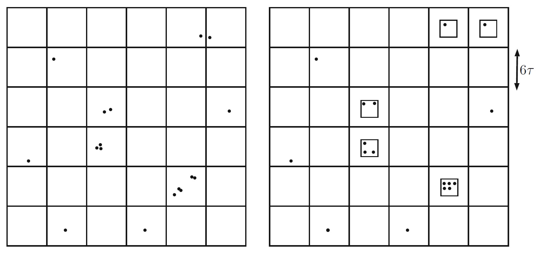
Figure 1: An unregularized configuration (left) and the regularization procedure applied to it (right). Taken from [26].

The set $\Lambda_{N}$ is now defined as $\Lambda_{N}=\alpha_{N^{-\frac{1}{d}}}\mathcal{R}\mathcal{A}$, where the family of point configurations $\mathcal{R}\mathcal{A}$ consists of the regularization procedure applied to each point configuration in $\mathcal{A}$.

By Lemma 5.9 of [26], we have that for any $i\in I$,

$$\lim_{\tau\to 0}\sup_{C\in{\rm Config}(K_{i})}d_{\rm Config}(C,\mathcal{R}C)=0.$$ (173)

On the other hand, by Claim 6.8 of [26] we have that

$$\limsup_{\tau\to 0,R\to\infty,N\to\infty}\sup_{C\in\mathcal{A}}d_{\mathcal{P}(\Omega\times{\rm Config})}(\overline{\mathbf{P}}_{N}(C),\overline{\mathbf{P}}_{N}(\mathcal{R}C))-\frac{1}{|I|}\sum_{i\in I}d_{\rm Config}(\theta_{x_{i}}\cdot C,\theta_{x_{i}}\cdot\mathcal{R}C)=0,$$ (174)

where $x_{i}$ is the center of the hypercube $K_{i}$. Putting together equations (173) and (174), we have that

$$\limsup_{\tau\to 0,R\to\infty,S\to\infty}\sup_{C\in\Lambda_{N}}d_{\mathcal{P}(\Omega\times{\rm Config})}(\overline{\mathbf{P}}_{N}(C),\overline{\mathbf{P}})\leq\delta.$$ (175)

Using Lemmas 6.10-6.16 in [26], we have that

$$\begin{split}\lim_{\tau\to 0}\liminf_{S\to\infty}\liminf_{R\to\infty}\lim_{N\to\infty}\frac{1}{N}\log\left(\mu_{\theta}^{\otimes N}(\Lambda_{N})\right)&\geq\liminf_{S\to\infty}\liminf_{R\to\infty}\lim_{N\to\infty}\frac{1}{N}\log\left(\mu_{\theta}^{\otimes N}(\alpha_{N^{-\frac{1}{d}}}\mathcal{A})\right)\\ &\geq-\overline{\rm Ent}[\overline{\mathbf{P}}|\overline{\mathbf{\Pi}}^{\mu_{\theta}}].\end{split}$$ (176)

Hence, for any ${\rm err}>0$, we can find $R,S,\tau$ such that

$$\lim_{N\to\infty}\frac{1}{N}\log\left(\mu_{\theta}^{\otimes N}(\Lambda_{N})\right)\geq-\overline{\rm Ent}[\overline{\mathbf{P}}|\overline{\mathbf{\Pi}}^{\mu_{\theta}}]-{\rm err}.$$ (177)

Items $1$ and $2$ are now proved, we move to the item $3$, which requires us to estimate the energy of such configurations.

Step 3[Energy estimate]

Throughout the proof, we will use the notation $\delta_{x}^{\epsilon}$ for the uniform probability measure on $B(x,\epsilon)$, and we will also use the notation $\delta_{\epsilon}=\delta_{0}^{\epsilon}$.

Substep 3.1

Let ${\rm emp}_{N}^{\epsilon}={\rm emp}_{N}\ast\delta_{\epsilon}$, for $\epsilon>0$ to be determined later. We will first derive an estimate for

$$\left|{\rm F}_{N}\left({\rm emp}_{N},\mu_{\theta}\right)-\mathcal{E}\left({\rm emp}_{N}^{\epsilon}-\mu_{\theta}\right)\right|.$$ (178)

For this, we write

$$\begin{split}&\left|{\rm F}_{N}\left({\rm emp}_{N},\mu_{\theta}\right)-\mathcal{E}\left({\rm emp}_{N}^{\epsilon}-\mu_{\theta}\right)\right|\\ =&\left|{\rm F}_{N}\left({\rm emp}_{N}\right),\mathcal{E}\left({\rm emp}_{N}^{\epsilon}\right)+2\mathcal{G}\left({\rm emp}_{N}-{\rm emp}_{N}^{\epsilon},\mu_{\theta}\right)\right|\\ \leq&2\left|\mathcal{G}\left({\rm emp}_{N}-{\rm emp}_{N}^{\epsilon},\mu_{\theta}\right)\right|+\left|\mathcal{G}^{\neq}\left({\rm emp}_{N}-{\rm emp}_{N}^{\epsilon},{\rm emp}_{N}\right)\right|+\left|\mathcal{G}\left({\rm emp}_{N}-{\rm emp}_{N}^{\epsilon},{\rm emp}_{N}^{\epsilon}\right)\right|\\ &\ \ \ \ \ +2\left|\mathcal{G}\left({\rm emp}_{N}-{\rm emp}_{N}^{\epsilon},\mu_{\theta}\right)\right|+\left|\sum_{i\neq j}\int h^{\delta_{x_{i}}-\delta_{x_{i}}^{\epsilon}}\delta_{x_{j}}\right|+\left|\sum_{i\neq j}\int h^{\delta_{x_{i}}-\delta_{x_{i}}^{\epsilon}}\delta_{x_{j}}^{\epsilon}\right|+\frac{1}{N}\mathcal{E}(\delta^{\epsilon})\end{split}$$ (179)

First we deal with the term $\left|\mathcal{G}\left({\rm emp}_{N}-{\rm emp}_{N}^{\epsilon},\mu_{\theta}\right)\right|$. Note that in order to show that
$\left|\mathcal{G}\left({\rm emp}_{N}-{\rm emp}_{N}^{\epsilon},\mu_{\theta}\right)\right|\to 0$, it suffices to show that $\left|\mathcal{G}\left(\delta_{x}-\delta_{x}^{\epsilon},\mu_{\theta}\right)\right|\to 0$ uniformly in $x$. To this end, take any $r>0$ and write

$$\mathcal{G}\left(\delta_{x}-\delta_{x}^{\epsilon},\mu_{\theta}\right)=\int_{|y-x|\leq r}h^{\delta_{x}-\delta_{x}^{\epsilon}}\mu_{\theta}(y)\,\mathrm{d}y+\int_{|y-x|\geq r}h^{\delta_{x}-\delta_{x}^{\epsilon}}\mu_{\theta}(y)\,\mathrm{d}y.$$ (180)

Note that

$$\left|\int_{|y-x|\leq r}h^{\delta_{x}-\delta_{x}^{\epsilon}}\mu_{\theta}(y)\,\mathrm{d}y\right|\leq 2\|\mu_{\theta}\|_{L^{\infty}}\int_{|y-x|\leq r+\epsilon}g(y)\,\mathrm{d}y.$$ (181)

For the remainder of the proof, we will use the notation

$$I(\epsilon)=\int_{\square_{\epsilon}}g(x)\,\mathrm{d}x,$$ (182)

and also the function

$$\Psi(\alpha,\beta)=\sup_{|x-y|<\beta,|x|>\alpha,|y|>\alpha}\left|g(x)-g(y)\right|.$$ (183)

Note that $\Psi(\alpha,\beta)$ is decreasing in $\alpha$, increasing in $\beta$, and for every $\alpha$, $\Psi(\alpha,\beta)\to 0$ as $\beta\to 0$ by uniform continuity (Property $3$ of $g$). We then have that

$$\left|\int_{|y-x|\geq r}h^{\delta_{x}-\delta_{x}^{\epsilon}}\mu_{\theta}(y)\,\mathrm{d}y\right|\leq\|\mu_{\theta}\|_{L^{1}}\Psi(r-\epsilon,\epsilon),$$ (184)

since for any $y$ such that $|x-y|>r$, we have that

$$\left|h^{\delta_{x}-\delta_{x}^{\epsilon}}(y)\right|\leq\Psi(r-\epsilon,\epsilon).$$ (185)

Putting together equations (181) and (184), we have that

$$\left|\mathcal{G}\left(\delta_{x}-\delta_{x}^{\epsilon},\mu_{\theta}\right)\right|\leq\|\mu_{\theta}\|_{L^{1}}\Psi(r-\epsilon,\epsilon)+\|\mu_{\theta}\|_{L^{\infty}}I(r+\epsilon).$$ (186)

We will now deal with the term $\mathcal{G}^{\neq}\left({\rm emp}_{N}-{\rm emp}_{N}^{\epsilon},{\rm emp}_{N}\right)$. The procedure is similar. Note that it suffices to show that $\mathcal{G}^{\neq}\left({\rm emp}_{N}-{\rm emp}_{N}^{\epsilon},x\right)\to 0$ uniformly for any $x$. For arbitrary $r>0$, we write

$$\mathcal{G}^{\neq}\left(\delta_{x}-\delta_{x}^{\epsilon},{\rm emp}_{N}\right)=\int_{y:0<|y-x|\leq r}h^{\delta_{x}-\delta_{x}^{\epsilon}}\,\mathrm{d}{\rm emp}_{N}(y)+\int_{y:|y-x|\geq r}h^{\delta_{x}-\delta_{x}^{\epsilon}}\,\mathrm{d}{\rm emp}_{N}(y),$$ (187)

and we have

$$\int_{y:|y-x|\geq r}h^{\delta_{x}-\delta_{x}^{\epsilon}}\,\mathrm{d}{\rm emp}_{N}(y)\leq\Psi(r-\epsilon,\epsilon).$$ (188)

On the other hand, it is not hard to prove that our construction (as a consequence of the regularization procedure) satisfies that for any $x$ and any $r>\tau N^{-\frac{1}{d}}$

$$\int_{B(x,\overline{r})}\,\mathrm{d}{\rm emp}_{N}\leq C_{S,R,\tau}r^{d},$$ (189)

where $C_{S,R,\tau}$ is a constant that depends only on $S,R,\tau$. In other words, the local density of points is uniformly bounded.

Therefore

$$\int_{y:0<|y-x|\leq r}h^{\delta_{x}-\delta_{x}^{\epsilon}}\,\mathrm{d}{\rm emp}_{N}(y)\leq C_{S,R,\tau}I(r+\epsilon).$$ (190)

Putting everything together, we have that

$$\mathcal{G}^{\neq}\left(\delta_{x}-\delta_{x}^{\epsilon},{\rm emp}_{N}\right)\leq C_{S,R,\tau}I(r+\epsilon)+\Psi(r-\epsilon,\epsilon).$$ (191)

Similarly, we have that

$$\left|\sum_{i\neq j}\int h^{\delta_{x_{i}}-\delta_{x_{i}}^{\epsilon}}\delta_{x_{j}}^{\epsilon}\right|\leq C_{S,R,\tau}I(r+\epsilon)+\Psi(r-\epsilon,\epsilon),$$ (192)

where $C_{S,R,\tau}$ depends on $S,R,\tau$.

Adding the errors we have that for any $r>0$,

$$\left|{\rm F}_{N}\left({\rm emp}_{N},\mu_{\theta}\right)-\mathcal{E}\left({\rm emp}_{N}^{\epsilon}-\mu_{\theta}\right)\right|\leq C_{S,R,\tau}I(r+\epsilon)+C\Psi(r-\epsilon,\epsilon)+\frac{1}{N}\mathcal{E}(\delta^{\epsilon}),$$ (193)

where $C$ is a constant that depends on $\mu_{\theta}$ and $C_{S,R,\tau}$ is a constant that depends, additionally. on $S,R,$ and $\tau$.

Substep 3.2

We now get an estimate for

$$\mathcal{E}\left({\rm emp}_{N}^{\epsilon}-\rho^{\epsilon}\right),$$ (194)

where

$$\rho^{\epsilon}=\rho\ast\delta^{\epsilon}.$$ (195)

For this, let $\eta>0$ to be determined later, and let $K_{i}$ be hypercubes of length $\eta$ which cover $\mathbb{T}^{d}$, and which are pairwise disjoint except for a set of measure $0$. Let $x\in\mathbb{T}^{d}$, with $x\in K_{j}$. Note that we can write

$$h^{{\rm emp}_{N}^{\epsilon}-\rho^{\epsilon}}=\int_{K_{j}}g^{\epsilon}(x-y)\,\mathrm{d}({\rm emp}_{N}-\rho)(y)+\sum_{i\neq j}\int_{K_{i}}g^{\epsilon}(x-y)\,\mathrm{d}({\rm emp}_{N}-\rho)(y),$$ (196)

where

$$g^{\epsilon}=g\ast\delta^{\epsilon}.$$ (197)

We will now get an estimate for each of the terms in the RHS of equation (196). Assume W.L.O.G. that

$${\rm emp}_{N}(K_{i})\leq\rho(K_{i}).$$ (198)

Then we have that

$$\begin{split}&\sum_{i\neq j}\left|\int_{K_{i}}g^{\epsilon}(x-y)\,\mathrm{d}({\rm emp}_{N}-\rho)(y)\right|\\ \leq&\sum_{i\neq j}\left|{\rm emp}_{N}(K_{i})\min_{y\in K_{i}}g^{\epsilon}(x-y)-\rho(K_{i})\max_{y\in K_{i}}g^{\epsilon}(x-y)\right|\\ \leq&\sum_{i\neq j}\left|\left[{\rm emp}_{N}(K_{i})-\rho(K_{i})\right]\max_{y\in K_{i}}g^{\epsilon}(x-y)\right|+\sum_{i\neq j}\left|\rho(K_{i})\left[\max_{y\in K_{i}}g^{\epsilon}(x-y)-\min_{y\in K_{i}}g^{\epsilon}(x-y)\right]\right|.\end{split}$$ (199)

We now introduce the function ${\rm Disc}(\eta,\delta,N)$, defined as

$${\rm Disc}(\eta,\delta,N)=\max_{X_{N}\in\Lambda_{N}}\max_{i}\left|{\rm emp}_{N}(K_{i})-\rho(K_{i})\right|.$$ (200)

Note that for any fixed $\eta>0$, we have that

$$\lim_{\delta\to 0}\lim_{N\to\infty}{\rm Disc}(\eta,\delta,N)=0,$$ (201)

since ${\rm emp}_{N}$ converges to $\rho$ weakly in the sense of probability measures. On the other hand,

$$\begin{split}\sum_{i\neq j}\left|\left[{\rm emp}_{N}(K_{i})-\rho(K_{i})\right]\max_{y\in K_{i}}g^{\epsilon}(x-y)\right|&\leq{\rm Disc}(\eta,\delta,N)\sum_{i\neq j}\left|\max_{y\in K_{i}}g^{\epsilon}(x-y)\right|\\ &\leq\frac{c_{g,\epsilon}}{\eta^{d}}{\rm Disc}(\eta,\delta,N),\end{split}$$ (202)

where $c_{g,\epsilon}$ is defined as

$$c_{g,\epsilon}=\max_{y\in\mathbb{T}^{d}}\left|g^{\epsilon}(y)\right|<\infty.$$ (203)

We now turn to the second term in the last line of (199). For this, let $r_{1}>0$ be big enough compared to $\eta$. Then we have that

$$\begin{split}&\sum_{i\neq j}\left|\rho(K_{i})\left[\max_{y\in K_{i}}g^{\epsilon}(x-y)-\min_{y\in K_{i}}g^{\epsilon}(x-y)\right]\right|\\ \leq&\sum_{i\neq j}\left|\|\rho\|_{L^{\infty}}\eta^{d}\left[\max_{y\in K_{i}}g^{\epsilon}(x-y)-\min_{y\in K_{i}}g^{\epsilon}(x-y)\right]\right|\\ =&\sum_{i\neq j,K_{i}\subset B(x,r_{1})}\left|\|\rho\|_{L^{\infty}}\eta^{d}\left[\max_{y\in K_{i}}g^{\epsilon}(x-y)-\min_{y\in K_{i}}g^{\epsilon}(x-y)\right]\right|\\ &\ \ \ \ \ \ \ \ +\sum_{i\neq j,K_{i}\cap(\mathbb{T}^{d}\setminus B(x,r_{1}))\neq\phi}\left|\|\rho\|_{L^{\infty}}\eta^{d}\left[\max_{y\in K_{i}}g^{\epsilon}(x-y)-\min_{y\in K_{i}}g^{\epsilon}(x-y)\right]\right|.\end{split}$$ (204)

Proceeding as in step 3.1, we have that

$$\begin{split}\sum_{i\neq j,K_{i}\subset B(x,r_{1})}\left|\|\rho\|_{L^{\infty}}\eta^{d}\left[\max_{y\in K_{i}}g^{\epsilon}(x-y)-\min_{y\in K_{i}}g^{\epsilon}(x-y)\right]\right|\leq 2\|\rho\|_{L^{\infty}}I(r_{1}+\epsilon),\\ \sum_{i\neq j,K_{i}\cap(\mathbb{T}^{d}\setminus B(x,r_{1}))\neq\phi}\left|\|\rho\|_{L^{\infty}}\eta^{d}\left[\max_{y\in K_{i}}g^{\epsilon}(x-y)-\min_{y\in K_{i}}g^{\epsilon}(x-y)\right]\right|\leq\|\rho\|_{L^{\infty}}\Psi(r_{1}-\eta,\eta).\end{split}$$ (205)

We now estimate the last term in equation (196), namely

$$\int_{K_{j}}g(x-y)\,\mathrm{d}({\rm emp}_{N}^{\epsilon}-\rho)(y).$$ (206)

Proceeding again as in step 3.1, we have that

$$\left|\int_{K_{j}}g(x-y)\,\mathrm{d}({\rm emp}_{N}^{\epsilon}-\rho)(y)\right|\leq(1+C_{S,R,\tau})I(\eta).$$ (207)

Putting everything together, we have that

$$h^{{\rm emp}_{N}^{\epsilon}-\rho^{\epsilon}}\leq\frac{c_{g,\epsilon}}{\eta^{d}}{\rm Disc}(\eta,\delta,N)+\|\rho\|_{L^{\infty}}\Psi(r_{1}-\eta,\eta)+\|\rho\|_{L^{\infty}}I(r_{1}+\epsilon)+(1+C_{S,R,\tau})I(\eta).$$ (208)

Substep 3.3[Conclusion of the energy estimate]

By adding and subtracting terms, we have that for any $\epsilon>0$,

$$\begin{split}&\left|{\rm F}_{N}({\rm emp}_{N},\mu_{\theta})-\mathcal{E}(\rho-\mu_{\theta})\right|\\ \leq&\left|{\rm F}_{N}({\rm emp}_{N},\mu_{\theta})-\mathcal{E}({\rm emp}_{N}^{\epsilon}-\mu_{\theta})\right|+\left|\mathcal{E}({\rm emp}_{N}^{\epsilon}-\mu_{\theta})-\mathcal{E}(\rho-\mu_{\theta})\right|\\ \leq&\left|{\rm F}_{N}({\rm emp}_{N},\mu_{\theta})-\mathcal{E}({\rm emp}_{N}^{\epsilon}-\mu_{\theta})\right|+\left|\mathcal{E}({\rm emp}_{N}^{\epsilon}-\mu_{\theta})-\mathcal{E}(\rho^{\epsilon}-\mu_{\theta})\right|\\ &\ \ \ \ \ \ \ +\left|\mathcal{E}(\rho-\mu_{\theta})-\mathcal{E}(\rho^{\epsilon}-\mu_{\theta})\right|.\end{split}$$ (209)

Using polar factorization for the quadratic form $\mu\to\mathcal{E}(\mu)$, we have

$$\begin{split}\left|\mathcal{E}({\rm emp}_{N}^{\epsilon}-\mu_{\theta})-\mathcal{E}(\rho^{\epsilon}-\mu_{\theta})\right|&=\left|\mathcal{G}\left({\rm emp}_{N}^{\epsilon}+\rho^{\epsilon}-2\mu_{\theta},{\rm emp}_{N}^{\epsilon}-\rho^{\epsilon}\right)\right|\\ &\leq 4\|h^{{\rm emp}_{N}^{\epsilon}-\rho^{\epsilon}}\|_{L^{\infty}}.\end{split}$$ (210)

Putting together all the previous estimates, we have that, for any $\epsilon,\eta,r,r_{1}>0$,

$$\begin{split}&\lim_{\delta\to 0}\lim_{N\to\infty}\left|{\rm F}_{N}({\rm emp}_{N},\mu_{\theta})-\mathcal{E}(\rho-\mu_{\theta})\right|\\ \leq&C_{S,R,\tau}I(r+\epsilon)+C\Psi(r-\epsilon,\epsilon)+\|\rho\|_{L^{\infty}}\Psi(r_{1}-\eta,\eta)+\|\rho\|_{L^{\infty}}I(r_{1}+\epsilon)+\\ &\ \ \ \ \ \ (1+C_{S,R,\tau})I(\eta)+\left|\mathcal{E}(\rho-\mu_{\theta})-\mathcal{E}(\rho^{\epsilon}-\mu_{\theta})\right|.\end{split}$$ (211)

Taking the limit $\epsilon\to 0$, then $\eta\to 0$, then $r,r_{1}\to 0$, we have that

$$\lim_{\delta\to 0}\lim_{N\to\infty}\left|{\rm F}_{N}({\rm emp}_{N},\mu_{\theta})-\mathcal{E}(\rho-\mu_{\theta})\right|=0.$$ (212)

Since the estimates are valid for any $X_{N}\in\Lambda_{N}$, we have that convergence is uniform.

This concludes the proof of Proposition 8.1.

∎

10 Appendix: Riesz and log gases at mid temperature

So far, we have discussed only general interactions at high temperature. It is natural to ask if it is possible to obtain a result valid in a more general temperature regime if we assume additional hypotheses on the interactions. If we specialize in Riesz interactions, then we can indeed obtain such a result. The results obtained in this section are not used in the rest of the paper, but we include them out of independent interest. For this section, we will work on $\mathbb{R}^{d}$, and not on $\mathbb{T}^{d}$. We start by recalling some well-known facts about Riesz gasses.

Lemma 10.1 (Equilibrium measure).

Let $g:\mathbb{R}^{d}\to\mathbb{R}$ be given by equations (4) and (5).

Assume that $V$ satisfies:

• $V$ is l.s.c. and bounded below.

• $$\lim_{x\to\infty}\frac{V(x)}{2}+g(x)=\infty.$$ (213)

• $V$ is finite on a set of positive measure.

Then $\mathcal{E}_{V}$ (given by equation (13)) has a unique minimizer in the set of probability measures, which we denote $\mu_{V}$. Furthermore, $\mu_{V}$ has compact support, which we denote $\Sigma$, and satisfies

$$\begin{cases}h^{\mu_{V}}+\frac{V}{2}+c\geq 0\\ h^{\mu_{V}}(x)+\frac{V}{2}(x)+c=0\ {\rm for}\ x\in\Sigma\end{cases}$$ (214)

for some $c\in\mathbb{R}$.

Proof.

See, for example, [37]. ∎

Lemma 10.2 (Splitting formula).

Assume that $g$ is given by equations (4) and (5), and that $V$ satisfies items $1-3$ of Lemma 10.1. Then for any point configuration $X_{N}$, the Hamiltonian can be rewritten (split) as

$$\mathcal{H}_{N}(X_{N})=N^{2}\mathcal{E}_{V}(\mu_{V})+2N\sum_{i=1}^{N}\zeta(x_{i})+N^{2}{\rm F}_{N}(X_{N},\mu_{V}),$$ (215)

where

$$\zeta(x)=h^{\mu_{V}}+\frac{V}{2}+c.$$ (216)

Proof.

See, for example, [37]. ∎

Definition 10.3 (Next-order partition function).

We define the mean-field next-order partition function $\widetilde{K}_{N,\beta}$ as

$$\widetilde{K}_{N,\beta}=\frac{Z_{N,\beta}}{\exp\left(-N^{2}\beta\mathcal{E}_{V}(\mu_{V})\right)}.$$ (217)

Now that we have recalled some well-known results, we state the main new result of this section.

Proposition 10.4.

Let $g$ be given by equations (4) and (5). Let $\overline{\mathbf{P}}_{N}$ be as in Definition 2.4, with $\Omega=\Sigma$. Assume that $\beta=N^{-\gamma}$, with $\gamma\in\left(\frac{d-2s}{d},1\right)$ (in the case of equation (4) we take $s=1$ for $d\geq 2$ and $s=\frac{1}{2}$ for $d=1$). Assume hypotheses (H1)-(H5) of [26]. Then the pushforward of $\mathbf{P}_{N,\beta}$ by $\overline{\mathbf{P}}_{N}$ satisfies an LDP in $\mathcal{P}(\mathbb{T}^{d}\times{\rm Config})$ at speed $N$ with rate function given by

$$\mathcal{F}(\overline{\mathbf{P}})=\begin{cases}\overline{\rm Ent}[\overline{\mathbf{P}}|\overline{\mathbf{\Pi}^{1}}]-\left({\rm ent}[\mu_{V}]-1+|\Sigma|\right)\ \ \textrm{if}\ \ \overline{\mathbf{P}}\in\mathcal{P}_{s,1}(\mathbb{T}^{d}\times{\rm Config})\\ \infty\ \ \ \ \ \ \ \ \ \ \ \ \ \ \ \ \ \ \ \ \ \ \ \ \ \ \ \ \ \ \ \ \ \ \ \ \ \ \ \textrm{if}\ \ \overline{\mathbf{P}}\notin\mathcal{P}_{s,1}(\mathbb{T}^{d}\times{\rm Config})\end{cases}$$ (218)

where

$$\mathcal{G}(\overline{\mathbf{P}})=\begin{cases}\overline{\rm Ent}[\overline{\mathbf{P}}|\overline{\mathbf{\Pi}^{1}}]\ \ \textrm{if}\ \ {\rm int}[\overline{\mathbf{P}}^{x}]=\mu_{V}(x)\ {\rm a.e.}\\ \infty\ \ \ \ \ \ \ \ \ \ \ \ \textrm{if not.}\end{cases}$$ (219)

Furthermore, $\widetilde{K}_{N,\beta}$ satisfies

$$\lim_{N\to\infty}\frac{\log\widetilde{K}_{N,\beta}}{N}\to-{\rm ent}[\mu_{V}].$$ (220)

Proof.

We introduce the constant

$$\omega_{N}=\int_{\mathbb{R}^{d}}\exp\left(-2N\beta\zeta(x)\right)\,\mathrm{d}x,$$ (221)

and also the probability measure

$$\rho_{N}(x)=\frac{1}{\omega_{N}}\exp\left(-2N\beta\zeta(x)\right).$$ (222)

Note that the Gibbs measure may be rewritten, for any point configuration $X_{N}$ as

$$\mathrm{d}\mathbf{P}_{N,\beta}(X_{N})=\frac{1}{\widetilde{K}_{N,\beta}}\exp\left(-N^{2}\beta{\rm F}_{N}(X_{N},\mu_{V})+N\log\omega_{N}\right)\Pi_{i=1}^{N}\rho_{N}(x_{i})\mathrm{d}X_{N}.$$ (223)

We also introduce the constant

$$c_{\omega,\Sigma}=\log|\omega|-|\Sigma|+1,$$ (224)

where

$$\omega:=\{x\in\mathbb{R}^{d}|\zeta(x)=0\}.$$ (225)

Note that if $\overline{\mathbf{P}}_{N}\to\overline{\mathbf{P}}$ and ${\rm int}[\overline{\mathbf{P}}^{x}]=\mu_{V}$ a.e. does not hold, then

$$\liminf_{N\to\infty}{\rm F}_{N}(X_{N},\mu_{V})>0,$$ (226)

see Subsection 5.4.

On the other hand, if ${\rm int}[\overline{\mathbf{P}}^{x}]=\mu_{V}$ a.e. then by [26] we have that, in the $1d$ log case

$$\liminf_{N\to\infty}N{\rm F}_{N}(X_{N},\mu_{V})+{\log N}\geq\overline{\mathbb{W}}(\overline{\mathbf{P}},\mu_{V}),$$ (227)

in the $2d$ log case

$$\liminf_{N\to\infty}N{\rm F}_{N}(X_{N},\mu_{V})+\frac{\log N}{2}\geq\overline{\mathbb{W}}(\overline{\mathbf{P}},\mu_{V}),$$ (228)

and in all other cases

$$\liminf_{N\to\infty}N^{\frac{2s}{d}}{\rm F}_{N}(X_{N},\mu_{V})\geq\overline{\mathbb{W}}(\overline{\mathbf{P}},\mu_{V}).$$ (229)

See [26] for a definition of $\overline{\mathbb{W}}$.

Furthermore, by Proposition 4.1 of [26],

$$\lim_{\epsilon\to 0}\lim_{N\to\infty}\frac{1}{N}\log\left(\rho_{N}^{\otimes N}\left(\overline{\mathbf{P}}_{N}\in B(\overline{\mathbf{P}},\epsilon)\right)\right)=-\overline{\rm Ent}[\overline{\mathbf{P}}|\overline{\mathbf{\Pi}}^{1}]-c_{\omega,\Sigma}.$$ (230)

Therefore, as long as $\overline{\mathbb{W}}(\overline{\mathbf{P}},\mu_{V})<\infty$ we have

$$\begin{split}&\lim_{\epsilon\to 0}\lim_{N\to\infty}\frac{1}{N}\log\left(\mathbf{P}_{N,\beta}\left(\overline{\mathbf{P}}_{N}\in B(\overline{\mathbf{P}},\epsilon)\right)\right)\\ \leq&\lim_{\epsilon\to 0}\lim_{N\to\infty}-\frac{1}{N}\log\left(\widetilde{K}_{N,\beta}\right)-N\beta\inf_{X_{N}:\overline{\mathbf{P}}_{N}\in B(\overline{\mathbf{P}},\epsilon)}{\rm F}_{N}(X_{N},\mu_{V})\\ &\ \ \ \ \ \ \ \ \ +\log\omega_{N}+\frac{1}{N}\log\left(\rho_{N}^{\otimes N}\left(\overline{\mathbf{P}}_{N}\in B(\overline{\mathbf{P}},\epsilon)\right)\right)\\ \leq&\lim_{N\to\infty}-\frac{1}{N}\log\left(\widetilde{K}_{N,\beta}\right)-\mathcal{G}(\overline{\mathbf{P}})+|\Sigma|-1,\end{split}$$ (231)

where we have used that if $N\beta\to\infty$ then

$$\lim_{N\to\infty}\log\omega_{N}=\log|\omega|$$ (232)

by Dominated Convergence Theorem. Similarly, if $\overline{\mathbb{W}}(\overline{\mathbf{P}},\mu_{V})<\infty$ then by Proposition 4.2 of [26], we have that

$$\lim_{\epsilon\to 0}\lim_{N\to\infty}\frac{1}{N}\log\left(\mathbf{P}_{N,\beta}\left(\overline{\mathbf{P}}_{N}\in B(\overline{\mathbf{P}},\epsilon)\right)\right)\geq\lim_{N\to\infty}-\frac{1}{N}\log\left(\widetilde{K}_{N,\beta}\right)-\mathcal{G}(\overline{\mathbf{P}})+|\Sigma|-1.$$ (233)

From this, we conclude that the pushforward of $\mathbf{P}_{N,\beta}$ by $\overline{\mathbf{P}}_{N}$ satisfies an LDP at speed $N$ with (the non-trivial part of the) rate function given by

$$\mathcal{F}(\overline{\mathbf{P}})=\mathcal{G}(\overline{\mathbf{P}})-\inf_{\overline{\mathbf{P}}^{*}\in\mathcal{P}_{s,1}(\Sigma\times{\rm Config})}\mathcal{G}(\overline{\mathbf{P}}^{*}),$$ (234)

and that $\widetilde{K}_{N,\beta}$ satisfies

$$\lim_{N\to\infty}\frac{\log\widetilde{K}_{N,\beta}}{N}\to|\Sigma|-1-\inf_{\overline{\mathbf{P}}^{*}\in\mathcal{P}_{s,1}(\Sigma\times{\rm Config})}\mathcal{G}(\overline{\mathbf{P}}^{*}).$$ (235)

In order to conclude, we note that the minimum of $\mathcal{G}(\overline{\mathbf{P}})$ is achieved at $\overline{\mathbf{P}}=\overline{\mathbf{\Pi}}^{\mu_{V}}$. By [26], Lemma 4.4, we have that the minimum is given by

$$\begin{split}\inf_{\overline{\mathbf{P}}^{*}\in\mathcal{P}_{s,1}(\Sigma\times{\rm Config})}\mathcal{G}(\overline{\mathbf{P}}^{*})&=\overline{\rm Ent}[\overline{\mathbf{\Pi}}^{\mu_{V}}|\overline{\mathbf{\Pi}}^{1}]\\ &=\int_{\Sigma}\mu_{V}(x)\log(\mu_{V}(x))-(\mu_{V}(x)-1)\,\mathrm{d}x\\ &={\rm ent}[\mu_{V}]-1+|\Sigma|.\end{split}$$ (236)

∎

Remark 5.

As mentioned before, it is not possible to guess the right rate function by starting from the LDP in [26] and simply dropping the energy term. However, $\mathcal{G}$ is the pointwise limit of the rate functions as $\theta\to 0$. As mentioned before, $\overline{\mathbb{W}}(\overline{\mathbf{P}},\mu_{V})=\infty$ if it is not true that ${\rm int}[\overline{\mathbf{P}}^{x}]=\mu_{V}(x)$ a.e. This implies that

$$\lim_{\theta\to 0}\theta\overline{\mathbb{W}}(\overline{\mathbf{P}},\mu_{V})+\overline{\rm Ent}[\overline{\mathbf{P}}|\overline{\mathbf{\Pi}}^{1}]=\mathcal{G}(\overline{\mathbf{P}})$$ (237)

for all $\overline{\mathbf{P}}\in\mathcal{P}_{s}(\Sigma\times{\rm Config})$.

11 Acknowledgements

DPG acknowledges support by the German Research Foundation (DFG) via the research unit FOR 3013 “Vector- and tensor-valued surface PDEs” (grant no. NE2138/3-1). We thank Sylvia Serfaty, Ed Saff, and particularly Gaultier Lambert for useful conversations.

References

- [1] A Alastuey and B Jancovici. On the classical two-dimensional one-component coulomb plasma. Journal de Physique, 42(1):1–12, 1981.
- [2] Luigi Ambrosio, Nicola Gigli, and Giuseppe Savare. Gradient flows in metric spaces and in the wasserstein space of probability measures. Lectures in Mathematics, ETH Zurich, Birkhäuser, 2005.
- [3] Scott Armstrong and Sylvia Serfaty. Local laws and rigidity for coulomb gases at any temperature. The Annals of Probability, 49(1):46–121, 2021.
- [4] Scott Armstrong and Sylvia Serfaty. Thermal approximation of the equilibrium measure and obstacle problem. In Annales de la Faculté des sciences de Toulouse: Mathématiques, volume 31, pages 1085–1110, 2022.
- [5] G Ben Arous and Alice Guionnet. Large deviations for wigner’s law and voiculescu’s non-commutative entropy. Probability theory and related fields, 108(4):517–542, 1997.
- [6] Robert J Berman. Determinantal point processes and fermions on complex manifolds: large deviations and bosonization. Communications in Mathematical Physics, 327(1):1–47, 2014.
- [7] Sergiy V Borodachov, Douglas P Hardin, and Edward B Saff. Discrete energy on rectifiable sets. Springer, 2019.
- [8] Paul Bourgade, László Erdős, and Horng-Tzer Yau. Bulk universality of general -ensembles with non-convex potential. Journal of mathematical physics, 53(9):095221, 2012.
- [9] Paul Bourgade, László Erdős, and Horng-Tzer Yau. Universality of general -ensembles. Duke Mathematical Journal, 163(6):1127–1190, 2014.
- [10] Paul Bourgade, Horng-Tzer Yau, and Jun Yin. Local circular law for random matrices. Probability Theory and Related Fields, 159(3):545–595, 2014.
- [11] Djalil Chafaï, Nathael Gozlan, and Pierre-André Zitt. First-order global asymptotics for confined particles with singular pair repulsion. The Annals of Applied Probability, 24(6):2371–2413, 2014.
- [12] Henry Cohn and Abhinav Kumar. Universally optimal distribution of points on spheres. Journal of the American Mathematical Society, 20(1):99–148, 2007.
- [13] Sacha Friedli and Yvan Velenik. Statistical mechanics of lattice systems: a concrete mathematical introduction. Cambridge University Press, 2017.
- [14] David García-Zelada. A large deviation principle for empirical measures on polish spaces: Application to singular gibbs measures on manifolds. In Annales de l’Institut Henri Poincaré, Probabilités et Statistiques, volume 55, pages 1377–1401. Institut Henri Poincaré, 2019.
- [15] David García-Zelada and David Padilla-Garza. Generalized transport inequalities and concentration bounds for riesz-type gases. arXiv preprint arXiv:2209.00587, 2022.
- [16] Hans-Otto Georgii. Gibbs measures and phase transitions. In Gibbs Measures and Phase Transitions. de Gruyter, 2011.
- [17] Steven M Girvin. Introduction to the fractional quantum hall effect. In The Quantum Hall Effect, pages 133–162. Springer, 2005.
- [18] Douglas P Hardin, Thomas Leblé, Edward B Saff, and Sylvia Serfaty. Large deviation principles for hypersingular riesz gases. Constructive Approximation, 48(1):61–100, 2018.
- [19] Adrien Hardy and Gaultier Lambert. Clt for circular beta-ensembles at high temperature. Journal of Functional Analysis, 280(7):108869, 2021.
- [20] B Jancovici, Joel L Lebowitz, and G Manificat. Large charge fluctuations in classical coulomb systems. Journal of statistical physics, 72(3):773–787, 1993.
- [21] Kurt Johansson. On fluctuations of eigenvalues of random hermitian matrices. Duke mathematical journal, 91(1):151–204, 1998.
- [22] Gaultier Lambert. Mesoscopic central limit theorem for the circular -ensembles and applications. Electronic Journal of Probability, 26:1–33, 2021.
- [23] Gaultier Lambert. Poisson statistics for gibbs measures at high temperature. In Annales de l’Institut Henri Poincaré, Probabilités et Statistiques, volume 57, pages 326–350. Institut Henri Poincaré, 2021.
- [24] Gaultier Lambert, Michel Ledoux, and Christian Webb. Quantitative normal approximation of linear statistics of -ensembles. The Annals of Probability, 47(5):2619–2685, 2019.
- [25] Thomas Leblé. Local microscopic behavior for 2d coulomb gases. Probability Theory and Related Fields, 169(3):931–976, 2017.
- [26] Thomas Leblé and Sylvia Serfaty. Large deviation principle for empirical fields of log and riesz gases. Inventiones mathematicae, 210(3):645–757, 2017.
- [27] Thomas Leblé, Sylvia Serfaty, and Ofer Zeitouni. Large deviations for the two-dimensional two-component plasma. Communications in Mathematical Physics, 350(1):301–360, 2017.
- [28] Cassio Neri. Statistical mechanics of the n-point vortex system with random intensities on a bounded domain. Annales de l’Institut Henri Poincaré C, 21(3):381–399, 2004.
- [29] David Padilla-Garza. Large deviation principle for local empirical measure of coulomb gases at intermediate temperature regime. arXiv preprint arXiv:2011.00480, 2020.
- [30] Mircea Petrache and Sylvia Serfaty. Crystallization for coulomb and riesz interactions as a consequence of the cohn-kumar conjecture. Proceedings of the American Mathematical Society, 148(7):3047–3057, 2020.
- [31] Dénes Petz and Fumio Hiai. Logarithmic energy as an entropy functional. Contemporary Mathematics, 217:205–221, 1998.
- [32] Nicolas Rougerie, Sylvia Serfaty, and Jakob Yngvason. Quantum hall phases and plasma analogy in rotating trapped bose gases. Journal of Statistical Physics, 154(1):2–50, 2014.
- [33] Nicolas Rougerie and Jakob Yngvason. Incompressibility estimates for the laughlin phase. Communications in Mathematical Physics, 336(3):1109–1140, 2015.
- [34] David Ruelle. A variational formulation of equilibrium statistical mechanics and the gibbs phase rule. Communications in Mathematical Physics, 5:324–329, 1967.
- [35] David Ruelle. Statistical mechanics of a one-dimensional lattice gas. Communications in Mathematical Physics, 9:267–278, 1968.
- [36] RR Sari and D Merlini. On the -dimensional one-component classical plasma: the thermodynamic limit problem revisited. Journal of Statistical Physics, 14(2):91–100, 1976.
- [37] Sylvia Serfaty. Coulomb gases and Ginzburg–Landau vortices. 2015.
- [38] Horst L Stormer, Daniel C Tsui, and Arthur C Gossard. The fractional quantum hall effect. Reviews of Modern Physics, 71(2):S298, 1999.
- [39] Salvatore Torquato. Hyperuniformity and its generalizations. Physical Review E, 94(2):022122, 2016.