s-LIME: Reconciling Locality and Fidelity in Linear Explanations

Abstract

The benefit of locality is one of the major premises of LIME, one of the most prominent methods to explain black-box machine learning models. This emphasis relies on the postulate that the more locally we look at the vicinity of an instance, the simpler the black-box model becomes, and the more accurately we can mimic it with a linear surrogate. As logical as this seems, our findings suggest that, with the current design of LIME, the surrogate model may degenerate when the explanation is too local, namely, when the bandwidth parameter $\sigma$ tends to zero. Based on this observation, the contribution of this paper is twofold. Firstly, we study the impact of both the bandwidth and the training vicinity on the fidelity and semantics of LIME explanations. Secondly, and based on our findings, we propose s-LIME, an extension of LIME that reconciles fidelity and locality.

1 Introduction

The pervasiveness of complex automatic decision-making nowadays has raised multiple concerns about the implications of AI for the values of fairness, trust, transparency, and privacy [2, 4, 13]. These concerns have propelled a plethora of work in explainable AI, a domain concerned with the design of models that can provide high-level comprehensive explanations for their answers. These models can be either explainable-by-design, or rely on external modules that compute explanations a posteriori. This need for post-hoc explainability is particularly compelling for sophisticated machine learning models, e.g., neural networks, whose logic is perceived as a black box by lay users.

One of the most prominent modules to compute post-hoc explanations for black-box supervised ML models is LIME [15]. This approach builds upon the notion of local feature attribution via a linear surrogate. Feature attribution means that the explanation quantifies the contribution of a set of features to the black box’s answer. This allows users to build a ranking of the features that play the biggest role in the model’s logic. We say the explanation is local because it only holds for a target instance and its vicinity. By focusing on a region of the feature space, LIME reduces the complexity of the black box and can approximate it using a surrogate sparse linear function whose coefficients constitute the feature attribution scores of the explanation. To learn this surrogate, LIME constructs a training set by generating artificial instances – called neighbors – around the target instance, and labeling them using the black box. The neighbors may not lie in the original feature space, but rather on a surrogate space that is meaningful to humans, e.g., image segments instead of pixels for images. The neighbors are weighted using an exponential kernel that depends on the distance to the target and a bandwidth parameter $\sigma\in\mathbb{R}^{+}$. The weighting process controls the level of locality of the explanation: the smaller $\sigma$ is, the more local the explanation becomes as closer neighbors are weighted higher than farther ones. More locality also implies focusing on a smaller region where the black box is presumably easier to approximate.

As logical as this sounds, our experiments suggest that small values of $\sigma$ can yield unfaithful or even trivially empty explanations. This counter-intuitive result has thus motivated this work, which brings two contributions: (a) A study of the impact of the bandwidth and the training vicinity on the fidelity and semantics of LIME, namely the meaning of the feature attribution scores; and (b) s-LIME, an extension of LIME that can solve the locality-fidelity paradox.

This paper is structured as follows. In Section 2 we introduce some background concepts and notations. We elaborate on our contributions in Sections 3 and 4. Section 5 presents an experimental evaluation of s-LIME. In Section 6 we survey the state of the art. Section 7 concludes the paper.

2 Preliminaries

Black Boxes and Linear Surrogates.

We assume our black box is a classification function $f:\mathbb{R}^{d}\rightarrow\mathbb{R}$ ($d\in\mathbb{Z}^{+}$) that predicts the probability that a target instance $x\in\mathbb{R}^{d}$ belongs to a given class. We denote by $x[i]$ the $i$-th feature of $x$. Conversely, the explanation $g:\mathbb{R}^{\hat{d}}\rightarrow\mathbb{R}$ ($\hat{d}\in\mathbb{Z}^{+}$) is a linear surrogate function that approximates $f$ in the locality of $x$, i.e., $g(\hat{x})=\hat{\alpha}_{0}+\sum_{1\leq i\leq\hat{d}}{\hat{\alpha}_{i}\hat{x}[i]}$. Note that $g$ may be defined on a surrogate space different from $f$’s. This implies the existence of a conversion function $\eta_{x}:\mathbb{R}^{\hat{d}}\rightarrow\mathbb{R}^{d}$ from the surrogate to the original space.

LIME.

In [15], the authors propose a model-agnostic method to compute local explanations for ML models in the form of sparse linear surrogates. LIME learns an explanation $g$ for a black box $f$ and an instance $x$ by solving the following minimization problem:

$$g=\mathop{argmin}_{g\in\mathcal{G}:\;\lVert\hat{\bm{\alpha}}\rVert_{0}\leqslant k}{\;\mathcal{L}_{x}(f,g)}$$ (1)

In other words, the surrogate $g$ is chosen such that it minimizes the error $\mathcal{L}_{x}$ w.r.t. the answers of $f$ on a neighborhood $\mathcal{X}$ around a target instance $x$. To keep the explanation meaningful to humans, LIME restricts itself to surrogate functions $g$ with less than $k$ non-zero parameters, where $k$ is a user-configurable hyper-parameter set by default to $6$. LIME does not assume access to the training data of the black box, therefore the neighbors $z\in\mathcal{X}$ take the form $z=\eta_{x}(\hat{z})$ where $\hat{z}\in\hat{\mathcal{X}}\subseteq\{0,1\}^{\hat{d}}$ is a synthetic instance that lies on a binary space. This space is interpretated as the presence or absence of features of the target $x$, so that $x=\eta_{x}(\hat{x})$ with $\hat{x}=\mathds{1}^{\hat{d}}$. The neighbors in $\hat{\mathcal{X}}$ are obtained by toggling off bits in $x$’s binary representation $\hat{x}$. When a bit is set to zero in the surrogate space, the conversion function $\eta_{x}$ must map the resulting vector to the original space. For images, this can be achieved by replacing the toggled-off super-pixels with a baseline monochrome segment or with a patch from another image [16]. LIME weighs the neighbors in $\hat{\mathcal{X}}$ according to a kernel function $\pi^{\sigma}_{x}$ (based on a distance $D$ and a bandwidth hyper-parameter $\sigma\in\mathbb{R}^{+}$) on the surrogate space, that is,

$$\mathcal{L}_{x}(f,g) =\sum_{\hat{z}\in\hat{\mathcal{X}}}{\pi_{x}^{\sigma}(\hat{z})(f(\eta_{x}(\hat{z}))-g(\hat{z}))^{2}}, \text{with }\pi^{\sigma}_{x}(\hat{z}) =\exp\left(\nicefrac{{-D(\hat{x},\hat{z})^{2}}}{{\sigma^{2}}}\right).$$

The hyper-parameter $\sigma$ controls the locality of the explanation so that smaller values give more weight to the instances that lie close to $\hat{x}$, i.e., those instances with fewer toggled-off bits. LIME does not make any assumptions about the inner-workings of $f$, however the distance $D$ and the conversion functions $\eta_{x}$ depend on $f$’s original space, which at the same time depends on the instances’ data type.

Quality Metrics.

The quality of the local surrogate $g$ is evaluated in terms of its fidelity, which can be measured via the surrogate’s adherence to the black box $f$ in the vicinity of $x$. Adherence is usually measured via the coefficient of determination R² [5, 17, 20]. The R² score measures the similarity between the predictions of both functions, compared to the variance of the black-box prediction. This coefficient lies in $(-\infty,1]$, where $R^{2}=1$ means $g$ fits $f$ perfectly and $R^{2}=0$ (respectively $R^{2}<0$) implies that $g$ is as accurate as (resp. less accurate than) the best constant model.

When a gold standard set $F_{f}(x)$ of important features is available, we can also calculate fidelity as the agreement between the explanation and the gold standard. This can be quantified via metrics such as recall [15], precision, or coverage [8]. Assuming the surrogate and the original feature spaces are identical, if the explanation $g$ for the target instance $x$ reports features $F_{g}(x)$ as the most important, the recall and precision of $g$ are respectively $\frac{|F_{f}(x)\cap F_{g}(x)|}{|F_{f}(x)|}$ and $\frac{|F_{f}(x)\cap F_{g}(x)|}{|F_{g}(x)|}$. Coverage can be used for data types where segments, i.e., conglomerates of contiguous features, are more meaningful to humans than individual features. Examples are time series and images. For those cases, the coverage is the proportion of the gold standard regions that overlap with the regions reported by the surrogate. Further specialized metrics have been proposed to measure the fidelity of pixel attribution explanations for image classifiers [9].

3 Locality vs. Fidelity

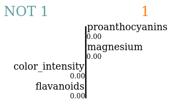
(a) $\sigma=0.1$

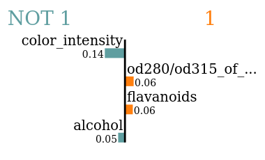
(b) $\sigma=0.75$

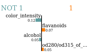
(c) $\sigma=100$

Figure 1: LIME explanations for three different bandwidths on the same instance of the wine dataset ($k=4$).

In this section we study the impact of two important elements of LIME on the fidelity and semantics of explanations, namely the bandwidth $\sigma$ and the neighborhood $\hat{\mathcal{X}}$.

3.1 The Paradox of Small Bandwidth

We illustrate the impact of $\sigma$ on the output of the tabular variant of LIME, which we use to explain a random forest classifier trained on the UCI wine dataset. Tabular LIME sets $\sigma=0.75$ with no further explanation. Changing $\sigma$ can, however, drastically change the resulting explanation as depicted in Figure 1. In particular, LIME computes null attribution coefficients when $\sigma=0.1$. Changing $\sigma$ from 0.75 to 100 rearranges the attribution ranking of the features.

To investigate the cause of this instability, we measure the adherence of the surrogate in $\hat{\mathcal{X}}$ as $\sigma$ varies for all the test instances of the dataset. We plot the results for two instances in Figure 2(a), where instance 2 is the example explained in Figure 1.

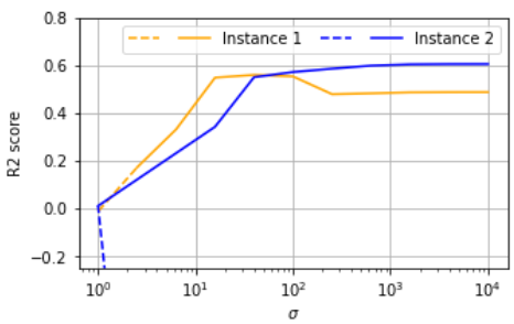
(a) R² vs. $\sigma$

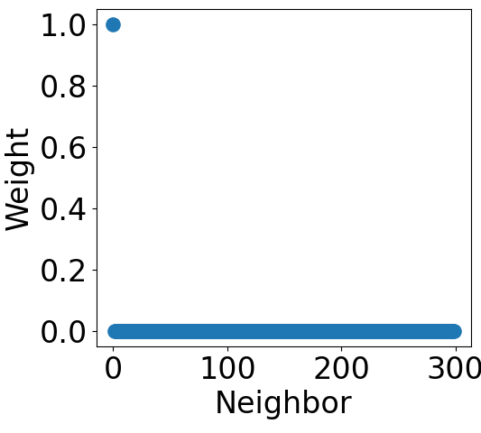
(b) $\sigma=0.1$

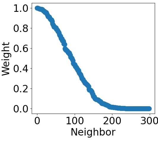
(c) $\sigma=100$

Figure 2: Left: Impact of the bandwidth $\sigma$ on the R² score of LIME for two instances of the wine dataset. Right: Distribution of the neighborhood weights for instance 2.

We recall that the R² score is calculated as $1-\nicefrac{{v_{r}(g)}}{{v(f)}}$, where $v_{r}(g)$ is the residual sum of squares of the surrogate $g$ and $v_{r}(f)$ is the total sum of squares of $f$’s answers. This means that the surrogate accounts for no more than 60% of the variability of the black box in $\hat{\mathcal{X}}$. The dashed regions of the curves indicate that the surrogate model has degenerated into a set of zero weights. This points out a counter-intuitive phenomenon: higher locality – achieved by making $\sigma$ small – yields poor explanations. We also observe that the R² may not increase monotonically with $\sigma$. Based on these observations, we devise two research questions that drive our contribution: (i) Why do seem locality and fidelity in opposition?, and (ii) what makes a good LIME explanation?

3.2 Why do Seem Locality and Fidelity in Opposition?

We investigate the cause of this paradox by means of Figures 2(b) and 2(c) that depict the distribution of weights for the neighbors of instance 2 for $\sigma=0.1$ and $\sigma=100$. In the first case, the LIME surrogate is a degenerated model that predicts a constant as hinted by Figure 2(a) and its corresponding explanation in Figure 1(a). Figure 2(b) tells us that the bulk of the weights is concentrated on the target instance. Such a phenomenon leads to a trivial training set. Even though locality is defined in terms of the entire set of instances in $\hat{\mathcal{X}}$, almost all of them are dispensable because they do not have any influence when learning the surrogate. The situation is less skewed for $\sigma=100$ (Figure 2(c)), which yields the non-trivial explanation in Figure 1(c).

From this analysis we conclude that the selection of $\sigma$ and the construction of $\hat{\mathcal{X}}$ must go in hand. We thus propose a strategy to jointly select them in Section 4.

3.3 What Makes a Good LIME Explanation?

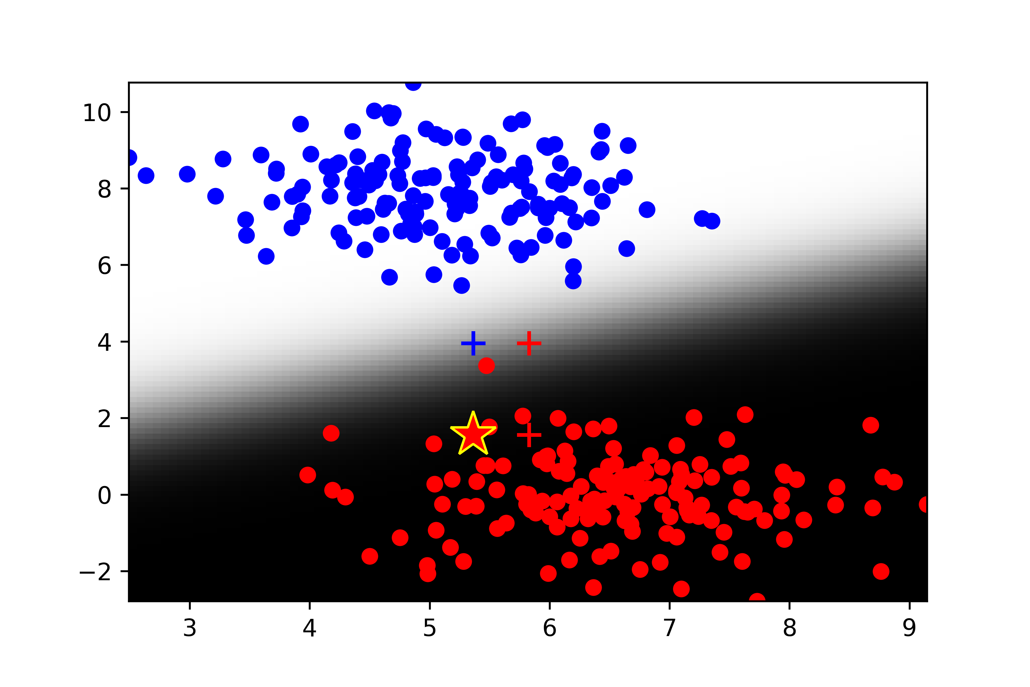
(a) Logistic Regression

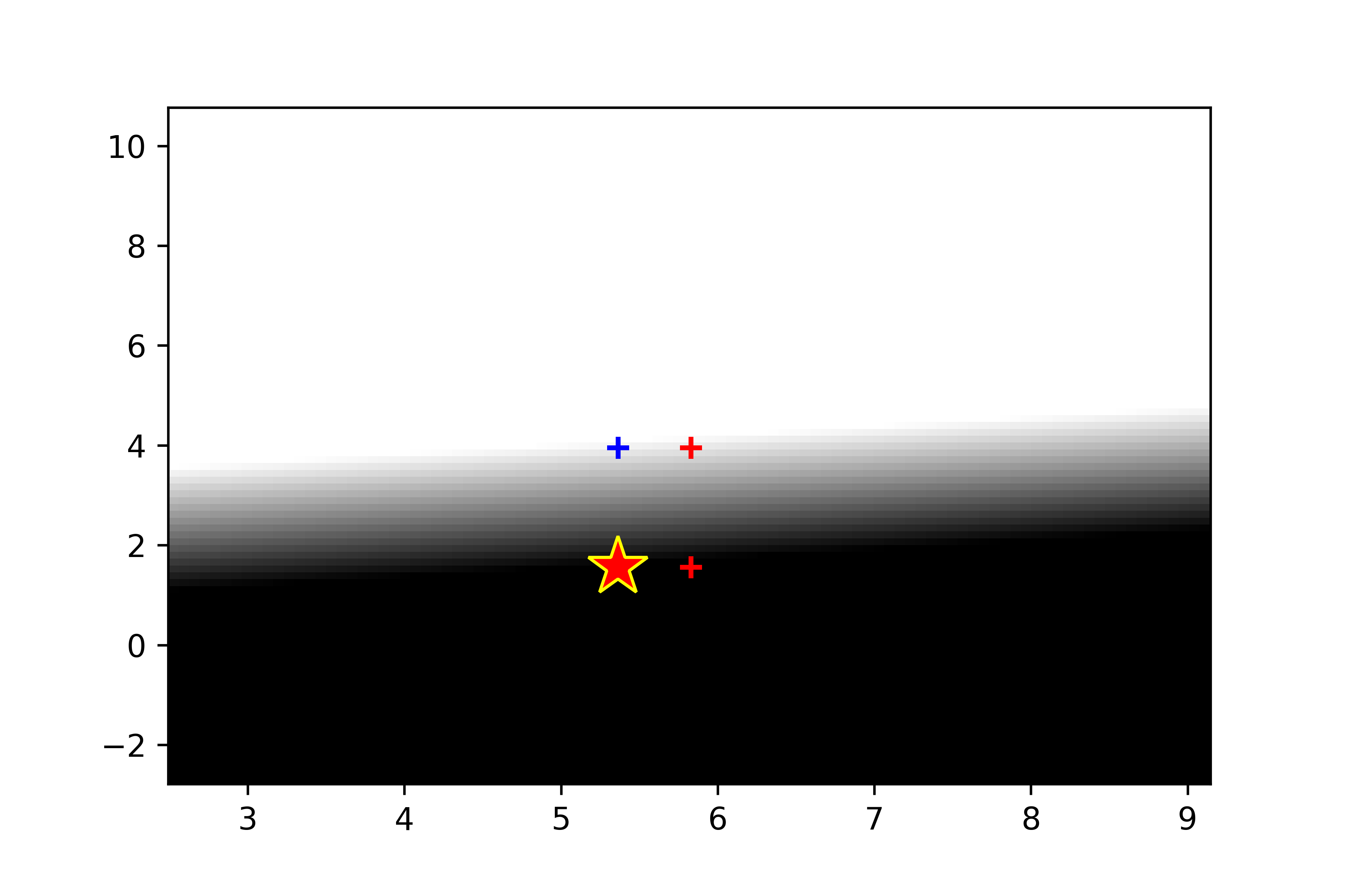
(b) $\sigma=0.5$

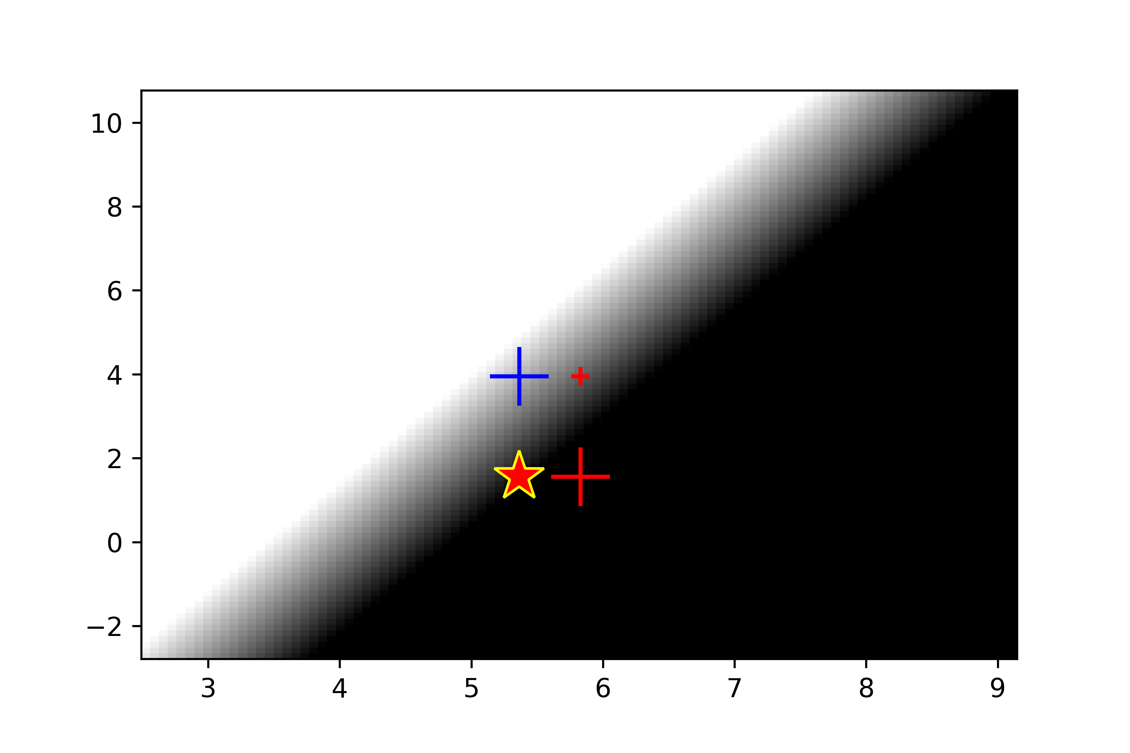
(c) $\sigma=1.0$

Figure 3: Left: A logistic regression classifier and a neighborhood (denoted by + marks) generated on a 2D discrete surrogate space. Center and right: Two LIME explanations. The gradient of each of these functions at the target example (denoted by the * mark) is orthogonal to the border between white area and black area. The explanation in the middle captures the black box’s gradient more faithfully.

The human aspects of interpretability are beyond the scope of this paper; instead this study is concerned with the quality and meaningfulness of explanations from a mathematical point of view. As suggested by [6], LIME computes a scaled version of the gradient $\nabla{}f$ for linear black boxes $f$. The scaling arises because the surrogate is learned on a finite number of neighbors in a discrete space, and the scaling factor depends on $x$, $\sigma$, $\eta_{x}$, and $\hat{\mathcal{X}}$. We argue that in the absence of a reference instance (as in [12, 18, 19]), explanations based on instantaneous gradients are meaningful and desirable because their semantics are well-defined: the surrogate gradient $\hat{\nabla{}}f(x)$ is the contribution of each surrogate feature to $f$’s change rate at point $x$. That said, LIME does not always estimate $\hat{\nabla{}}f$ accurately as suggested by Figure 3. The figures show that the weights associated to the neighbors may yield an estimation that differs largely from the black box’s actual gradient in Figure 3(a).

4 s-LIME

To tackle the locality-fidelity paradox explained in Section 3.1, we introduce an extension of LIME, called s-LIME (Smoothed LIME), that we detailed in the following.

4.1 Generic Algorithm

Algorithm 1 s-LIME applied to black-box function $f$ at target instance $x$

1:Conversion function $\eta_{x}$, distribution $\nu_{\sigma}$ on the surrogate space

2:Number $k$ of features in the explanation, number $n$ of local examples

3:$\hat{\mathcal{X}}\leftarrow\left\{\hat{z}^{(i)}:i=1,\dots,n\right\}$, where $\hat{z}^{(i)}\sim\nu_{\sigma}$ for $i=1,\dots,n$

4:return $\mathop{argmin}_{g\in\mathcal{G}:\;\lVert\hat{\bm{\alpha}}\rVert_{0}\leqslant k}\sum_{\hat{z}\in\hat{\mathcal{X}}}\left(f(\eta_{x}(\hat{z})),g(\hat{z})\right)^{2}$

LIME may compute degenerated explanations due to two main factors: (i) the discreteness of the surrogate space, and (ii) the fact that instance generation and weighting are decoupled. Indeed, LIME first generates a discrete neighborhood $\hat{\mathcal{X}}$ (independently of $\sigma$), and then weighs the instances in $\hat{\mathcal{X}}$ using $\pi^{\sigma}_{x}$. In the extreme cases when $\sigma$ tends to zero, the weighting is concentrated on $\hat{x}$.

To prevent this skewed concentration of weights, we control the locality of the explanation in a single step (see Algorithm 1). Hence, we define the neighbors in the continuous space $[0,1]^{\hat{d}}$ and populate $\hat{\mathcal{X}}$ with examples $\hat{z}$ whose distance $D$ to $\hat{x}$ is of the same magnitude as $\sigma$. Concretely, the neighborhood $\hat{\mathcal{X}}=\{\hat{z}^{(1)},\dots,\hat{z}^{(n)}\}$ consists of $n$ equally-weighted instances drawn independently from a distribution $\nu_{\sigma}$. Such a design decision enables $g$ to approximate $\hat{\nabla{}}f$ when $\sigma$ tends to zero, without hindering interpretability: $g$ still combines the contributions of the surrogate features linearly, and we can still confer an interpretable meaning to the neighbors as later explained in Section 4.4. Moreover, this allows controlling locality via the bandwidth of the neighborhood distribution, and not anymore through an a-posteriori weighting.

Note that s-LIME also requires the definition of new conversion functions $\eta_{x}$ as $\hat{\mathcal{X}}$ is now a subset of the continuous space $[0,1]^{\hat{d}}$ instead of the discrete space $\{0,1\}^{\hat{d}}$. In Section 4.4 we provide examples of proper distributions $\nu_{\sigma}$ and functions $\eta_{x}$ for images, time series, and tabular data.

4.2 s-LIME Subsumes LIME

Lemma 1

Let $f$ be a function and $x$ a target instance. There is a distribution $\nu_{\sigma}$ over $[0,1]^{\hat{d}}$ such that LIME and s-LIME are minimizing the same expected loss function.

Proof

LIME outputs a function $g$ that minimizes the loss $\mathcal{L}_{x}(f,g)$ which is the residual sum of squares of the examples drawn from a distribution $\nu$. The expectation of this loss function w.r.t. to a random neighborhood is $\mathds{E}_{\hat{z}\sim\nu}\left[\pi_{x}^{\sigma}(\hat{z})\left(f(\eta_{x}(\hat{z}))-g(\hat{z})\right)^{2}\right].$ Remark that $\nu$ is a distribution on the finite space $\{0,1\}^{\hat{d}}$, then $\nu=\sum_{\hat{z}\in\{0,1\}^{\hat{d}}}w_{\nu}(\hat{z})\delta(\hat{z})$, where $\delta(\hat{z})$ is the Dirac distribution at point $\hat{z}$, and $w_{\nu}(\hat{z})$ is a positive real number.

Similarly, s-LIME returns the linear surrogate $g$ that minimizes a loss with expectation $\mathds{E}_{\hat{z}\sim\nu_{\sigma}}\left[\left(f(\eta_{x}(\hat{z}))-g(\hat{z})\right)^{2}\right].$ Let $Z$ be $\sum_{\hat{z}\in\{0,1\}^{\hat{d}}}\pi_{x}^{\sigma}(\hat{z})w_{\nu}(\hat{z})$. If we consider s-LIME with generating distribution $\nu_{\sigma}=\nicefrac{{1}}{{Z}}\sum_{\hat{z}\in\{0,1\}^{\hat{d}}}\pi_{x}^{\sigma}(\hat{z})w_{\nu}(\hat{z})\delta(\hat{z})$, then

$$\mathds{E}_{\hat{z}\sim\nu_{\sigma}}\left[\left(f(\eta_{x}(\hat{z}))-g(\hat{z})\right)^{2}\right] =\sum_{\hat{z}\in\{0,1\}^{\hat{d}}}\frac{\pi_{x}^{\sigma}(\hat{z})w_{\nu}(\hat{z})}{Z}\left(f(\eta_{x}(\hat{z}))-g(\hat{z})\right)^{2}$$

$$=\frac{1}{Z}\mathds{E}_{\hat{z}\sim\nu}\left[\pi_{x}^{\sigma}(\hat{z})\left(f(\eta_{x}(\hat{z}))-g(\hat{z})\right)^{2}\right],$$

which concludes the proof.

Remark 1

It follows from Lemma 1 that s-LIME may be used as a placeholder for LIME. Still, the proposed distribution $\nu_{\sigma}$ is practical only when $d$ is small, or when $\nu_{\sigma}$ corresponds to a well-known distribution. Otherwise, storing the $2^{\hat{d}}$ coefficients $\pi_{x}^{\sigma}(\hat{z})w_{\nu}(\hat{z})$ is unpractical. Anyway, we demonstrate in Section 5 that s-LIME with a continuous distribution is more faithful than LIME.

4.3 s-LIME and the Gradient of the Black-Box Function

Let us assume the surrogate function $f\circ\eta_{x}$ to be differentiable at $\hat{x}$. Let us also denote by $\hat{\bm{\alpha}}$ the weights of the linear model returned by s-LIME when we drop the sparseness constraint. Then for any family of continuous distributions $\nu_{\sigma}$ on $[0,1]^{\hat{d}}$, such that their mass concentrates on $\hat{x}$ when $\sigma$ tends to zero, $\hat{\bm{\alpha}}$ tends to the gradient $\hat{\nabla}f(x)$ of $f\circ\eta_{x}$ at point $\hat{x}$. An example of such family of distributions is the set $\{\mathcal{N}\left(\hat{x},\sigma^{2}\boldsymbol{I}\right),\sigma\in\mathbb{R}^{+}\}$ of Gaussian distributions centered at $\hat{x}$ with variance $\sigma^{2}\boldsymbol{I}$, where $\boldsymbol{I}$ is the identity matrix.

This property has two main implications. First, while LIME degenerates as $\sigma$ approaches zero, s-LIME remains well-defined for any value of $\sigma$. Secondly, we know what s-LIME is targeting when we look locally at $\hat{x}$: $\hat{\nabla}f(x)$.

Remark 2

There are settings for which surrogate gradients are meaningless: piece-wise constant functions such as random forests. In such a scenario, s-LIME outputs a zero gradient as soon as the bandwidth of the generating distribution is small enough. While the weights returned by s-LIME are mathematically consistent for such kinds of models, they are useless as they carry on information that is too local. If that is the case, users may pick a higher value for $\sigma$, or resort to a rule-based surrogate [16].

4.4 s-LIME Implementations

Let us now discuss examples of concrete distributions $\nu_{\sigma}$ and functions $\eta_{x}$. The generating distribution $\nu_{\sigma}$ is the same for image and time series datasets: the uniform distribution on $[1-\sigma,1]^{\hat{d}}$, with $\sigma\in(0,1]$. As needed, this distribution concentrates around the surrogate target $\hat{x}=\mathds{1}^{\hat{d}}$ when $\sigma$ tends to zero.

In regards to the conversion function $\eta_{x}$, we recall that for both images [15] and time series [8], LIME splits the original instance into $\hat{d}$ contiguous regions, namely super-pixels for images or fragments of fixed size for time series. Those regions define the features of the surrogate space. Given a neighbor $\hat{z}\in\hat{\mathcal{X}}$ and a surrogate feature $j$, we can project $\hat{z}$ back to the original space by interpolating the original features of the target $x$ with a baseline $x_{0}$, i.e., $\eta_{x}(\hat{z})[i]=(1-\hat{z}[j])x_{0}+\hat{z}[j]x[i]$ for all the original features $i$, i.e., pixels or time measures, covered by segment $j$. We set $x_{0}=0$ in our experiments, i.e., the interpolation is done w.r.t. a black image and a null time series.

Finally, for tabular data we consider one surrogate feature per original feature. Therefore, the generating distribution $\nu_{\sigma}$ is the centered multivariate Gaussian distribution with covariance $\sigma^{2}\boldsymbol{I}$, and the function $\eta_{x}(\hat{z})=x+\hat{z}$.

Remark 3

The design of a proper distribution $\nu_{\sigma}$ and a proper function $\eta_{x}$ requires the black-box model to handle examples living in a continuous space. As a consequence, s-LIME cannot be defined for text data.

5 Experiments

We now show-case the impact of the bandwidth $\sigma$ on the fidelity of LIME and s-LIME explanations. We first detail our experimental setup and then elaborate on our findings.

5.1 Experimental Settings

Datasets and Black Boxes.

We conduct our experiments on a variety of datasets, comprising Cifar10 [10] and MNIST [11] for image data, the FordA and StarlightCurves time series datasets from the UEA & UCR Time Series Classification Repository, and the Compas and Diabetes datasets from the UCI Machine Learning Repository for tabular data. We also consider a selection of black-box models, which may be smooth or piece-wise constant, simple or complex, interpretable or not.

Protocol and Metrics.

For each combination of dataset, model, and explanation module, we compute the average value of the experimental metrics for different values of $\sigma$ on the test instances of the dataset. The experimental metrics were introduced in Section 2: the $R^{2}$ score for all models, and the precision/recall or the coverage for the interpretable models, i.e., those for which a ground truth is available. All these metrics take values either in $(-\infty,1]$ or in $[0,1]$, and higher values denote higher fidelity.

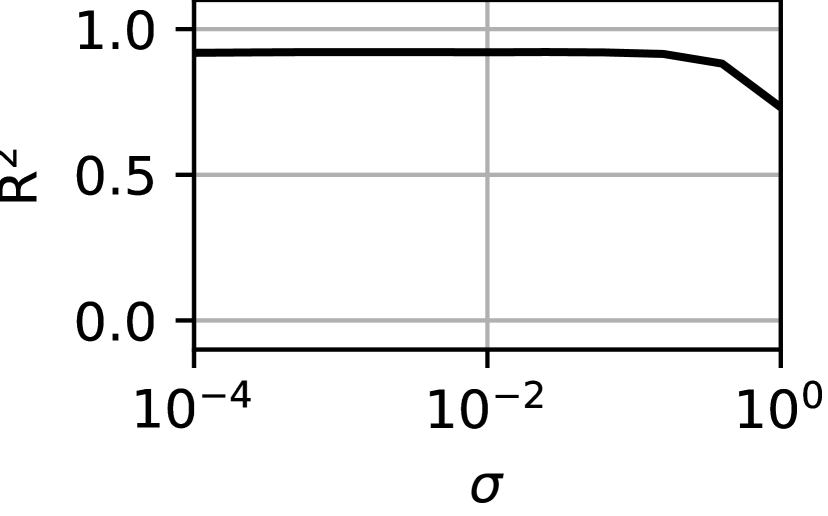
(a) s-LIME on LS

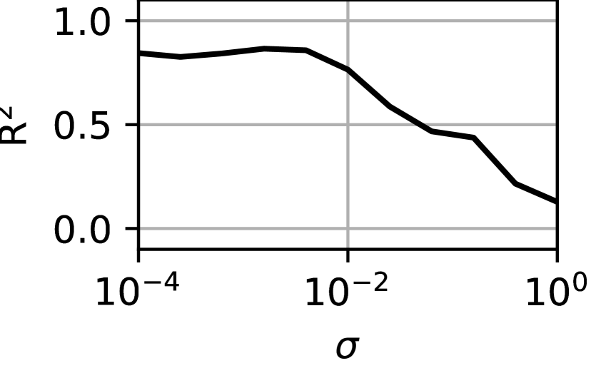
(b) s-LIME on RES.

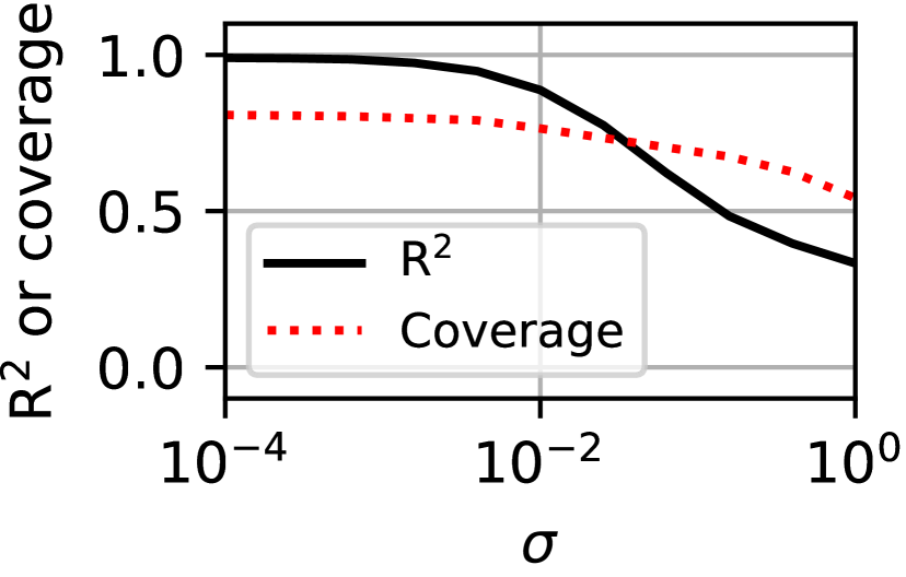
(c) s-LIME on LR

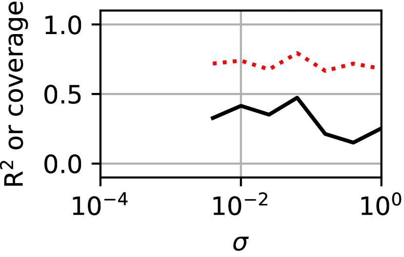
(d) s-LIME on FS

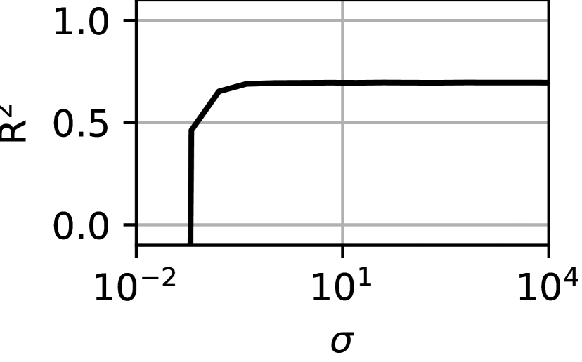
(e) LIME on LS

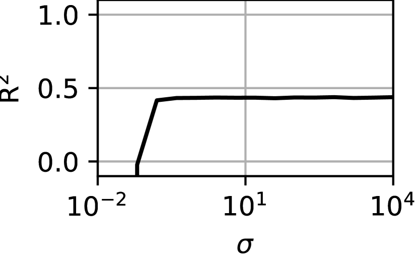
(f) LIME on RESNET

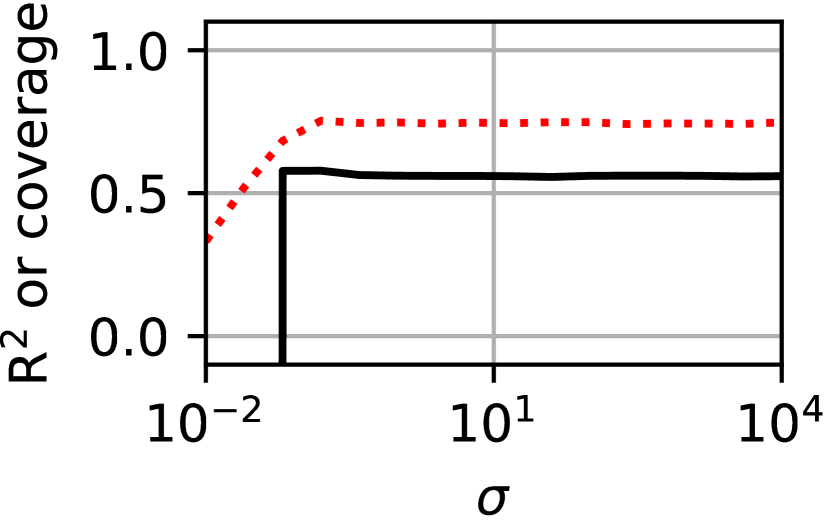
(g) LIME on LR

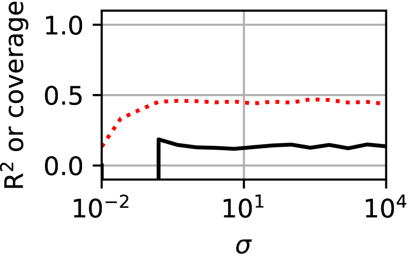
(h) LIME on FS

Figure 4: $R^{2}$ and coverage vs. $\sigma$ on the StarlightCurves dataset. Each subplot corresponds to a couple (explainer, dataset). The plotted results are averaged on the instances of the test dataset. Recall that for s-LIME $\sigma$ is defined in $(0,1]$.

5.2 Impact of $\sigma$

To study the impact of $\sigma$ on the fidelity of the LIME and s-LIME explanations, we plot the surrogate’s adherence on the StarlightCurves dataset for several black-box models all using 100 random shapelets as input features. The models include Learning Shapelets (LS) [7], RESNET [21], Fast Shapelets (FS) [14], and a sparse logistic regression (LR, with $L_{1}$-regularization to enforce at most 10 features). The results are depicted in Figure 4. We set $k=6$ for the number of features in explanations [15].

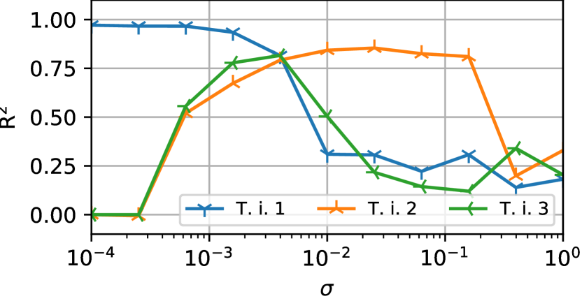
(a) s-LIME on RESNET

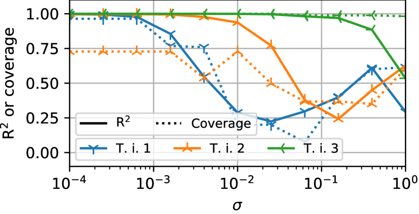
(b) s-LIME on LR

Figure 5: $R^{2}$ and coverage vs. $\sigma$ on the StarlightCurves dataset. Each subplot corresponds to a couple (explainer, dataset). Each curve corresponds to one target instance.

We observe that very local s-LIME neighborhoods lead to higher adherence and coverage, except for FS. This translates into more faithful explanations as $\sigma$ approaches zero, where LIME cannot deliver proper explanations. In contrast, LIME achieves higher adherence and coverage for FS, because this model is a decision tree. Hence, the decision function is piece-wise constant and its gradient is zero almost every-where. When $\sigma$ is small enough, s-LIME recovers this gradient and returns an explanation with null coefficients, which has little practical value. That said, a wider locality can still yield a more informative explanation.

We also remark that, for complex models, the best value for $\sigma$ may depend on the target instance. This is corroborated by Figure 5 that shows the disaggregated results for 3 instances on RESNET, a deep neural network. We can observe that the adherence is maximal when $\sigma$ is equal $10^{-4}$, $3\times 10^{-3}$, and $2\times 10^{-2}$ respectively. On the other hand, the same values of $\sigma$ are optimal for all examples on a simpler LR model.

Finally, we highlight that the coverage peaks when the adherence is maximal both at the instance (Figure 5(b)) and dataset level (Figures 4(cdgh)). This shows the pertinence of the $R^{2}$ score as metric to select the right level of locality.

Table 1: Best average recall and precision, or coverage (std. in parentheses) on different datasets and interpretable black-box classifiers.

Data type	Dataset	Model	s-LIME		LIME
			Rec. or Cov.	Precision	Rec. or Cov.	Precision
Timeseries	FordA	LR on shapelets	0.87 (0.15)	- (-)	0.73 (0.17)	- (-)
		Fast Shapelets	0.51 (0.30)	- (-)	0.49 (0.27)	- (-)
	Starlight-	LR on shapelets	0.81 (0.17)	- (-)	0.75 (0.17)	- (-)
	Curves	Fast Shapelets	0.68 (0.19)	- (-)	0.45 (0.15)	- (-)
Tabular data	Diabetes	Logistic Reg.	1.00 (0.00)	1.00 (0.00)	0.88 (0.12)	0.88 (0.12)
		Dec. Tree	0.95 (0.13)	0.81 (0.20)	0.94 (0.14)	0.80 (0.20)
	Compas	Logistic Reg.	1.00 (0.00)	1.00 (0.00)	0.52 (0.21)	0.52 (0.21)
		Dec. Tree	0.66 (0.33)	0.25 (0.00)	0.65 (0.33)	0.33 (0.00)

Table 2: Best average $R^{2}$ (std. in parentheses) on different datasets and black-box classifiers. MLP stands for a neural network with one hidden layer composed of 100 neurons and logistic sigmoid activation function. Column Int. indicates interpretable black-box models ($\checkmark$). FS, DT and RF are put aside as they are piecewise constant models.

Data type	Model	Int.	$k$	s-LIME	LIME	$k$	s-LIME	LIME
Images			MNIST			Cifar10
	Alexnet		10	0.80 (0.28)	0.58 (0.20)	10	0.84 (0.10)	0.55 (0.25)
	VGG16		10	0.56 (0.43)	0.57 (0.21)	10	0.69 (0.13)	0.50 (0.27)
Timeseries			FordA			StarlightCurves
	Learning Shapelets		6	0.84 (0.08)	0.57 (0.15)	6	0.92 (0.07)	0.70 (0.07)
	RESNET		6	0.73 (0.20)	0.10 (1.05)	6	0.87 (0.15)	0.44 (0.15)
	LR on Shapelets	✓	6	1.00 (0.01)	0.56 (0.13)	6	0.99 (0.02)	0.58 (0.12)
	Fast Shapelets	✓	6	0.15 (0.18)	0.19 (0.14)	6	0.25 (0.13)	0.19 (0.16)
Tabular data			Diabetes			Compas
	Logistic Regression	✓	4	1.00 (0.00)	0.99 (0.01)	11	1.00 (0.00)	0.42 (0.23)
	MLP		4	0.97 (0.03)	0.72 (0.13)	6	0.79 (0.01)	0.31 (0.16)
	Decision Tree	✓	3	0.46 (0.09)	0.46 (0.10)	3	0.34 (0.00)	0.36 (0.00)
	Random Forest		4	0.62 (0.03)	0.58 (0.12)	6	0.30 (0.01)	0.30 (0.02)

5.3 Fidelity Analysis

Tables 1 and 2 show the average scores obtained by s-LIME and LIME when $\sigma$ is selected to maximize the aggregated adherence ($R^{2}$ score) in the test instances of the experimental datasets. Table 1 shows recall, precision, and coverage for the interpretable models, whereas Table 2 provides the $R^{2}$ score for all models.

Firstly, we remark that s-LIME’s explanations are strictly more faithful than LIME’s except for piecewise constant models (FS, DT, and RF). That said, this does not prevent s-LIME from achieving higher adherence for such models on some datasets when we look at a larger vicinity.

Secondly, the $R^{2}$ score is a good proxy to predict the best neighborhood in terms of recall, precision, or coverage. This is a strong result from an application point of view. Practitioners are mostly interested by the features that are actually used by the black-box model. For cases where those actual features are unknown, the $R^{2}$ score enables the computation of faithful linear explanations that can identify the important features.

6 Related Work

Feature-attribution explanations.

Methods such as DeepLIFT [18], Integrated Gradients (IG) [19], SHAP [12], or LIME [15] compute importance local attribution scores for the features of a black-box ML model. Among those, SHAP and LIME are model-agnostic and compute linear surrogates learned from artificial neighbors. Despite these similarities, the semantics of their explanations are different as confirmed by existing studies [1]. While LIME approximates – often coarsely – the instantaneous gradient of the black box w.r.t. the input features [6], SHAP computes – or rather approximates – the Shapley values [12], which quantify the feature contributions to the difference between the model’s answer on a baseline instance and the target. The baseline depends on the use case, e.g., a single-color image (represented by the vector $\mathbb{0}^{\hat{d}}$ in the surrogate space). This makes SHAP and LIME complementary methods rather than competitors.

LIME Extensions.

An important body of literature has studied the impact of the different components and parameters of LIME on the quality of the explanations. This has led to multiple extensions of the original LIME algorithm. As opposed to this work, some extensions [17, 22, 20] tackle the instability of LIME, i.e., the fact that two executions of the algorithm with the same input may not deliver the same explanation. This instability originates from the randomness in the different steps of the approach, e.g., sampling in the surrogate space, non-deterministic conversion functions, etc. On those grounds, the techniques to tackle instability are diverse. ALIME [17], for example, resorts to a denoising auto-encoder to create a surrogate space that characterizes the data manifold more accurately. DLIME [22], in contrast, applies hierarchical agglomerative clustering on the training instances to identify the closest neighbors of the target and use them to learn the surrogate. In another line of thought, the authors of OptiLIME [20] study the relationship between the bandwidth $\sigma$, the adherence, and the instability of LIME. Similar to our work, the authors highlight the importance of choosing the right $\sigma$ in a per-instance basis. Moreover, they show an inverse relationship between $\sigma$ and explanation instability. This observation constitutes the basis of a method to select the bandwidth $\sigma$ that yields the best trade-off between adherence and instability. We highlight that all these approaches have been proposed only for tabular data, and that none of them takes into account recall, precision, or coverage fidelity.

Other extensions of LIME have focused entirely on improving fidelity. ILIME [5] proposes the use of influence functions in order to up-weight the neighbors that play a higher role in the linear fit of the surrogate. QLIME-A [3] proposes to extend the local surrogate to report quadratic relationships for cases where a linear surrogate is still inaccurate. While quadratic functions do exhibit higher fit capabilities, their interpretability in general settings is debatable.

7 Conclusion

In this paper we have introduced s-LIME, an extension of LIME that reconciles locality and fidelity for linear explanations. We argue that LIME can produce degenerated explanations as locality – controlled through the bandwidth $\sigma$ – increases. We solve this paradox by means of a new neighbor generation process on a continuous surrogate space. Our experiments on image, time series, and tabular data suggest that this strategy can provide even more faithful linear explanations with gradient-compliant semantics that are not affected by high locality. As a future work, we envision to investigate the fidelity of s-LIME explanations with other generating distributions and conversion functions, as well as to study the impact on the stability of the explanations.

7.0.1 Acknowledgements

This research was partially supported by the Inria Project Lab “Hybrid Approaches for Interpretable AI” (HyAIAI), the project “Framework for Automatic Interpretability in Machine Learning” financed by the French National Research Agency (ANR JCJC FAbLe), and the network on the foundations of trustworthy AI, integrating learning, optimisation, and reasoning (TAILOR) financed by the EU’s Horizon 2020 research and innovation program under agreement 952215.

References

- [1] Amparore, E., Perotti, A., Bajardi, P.: To Trust or not to Trust an Explanation: Using LEAF to Evaluate Local Linear XAI Methods. PeerJ Computer Science 7 (2021). https://doi.org/10.7717/peerj-cs.479, http://dx.doi.org/10.7717/peerj-cs.479
- [2] Bodria, F., Giannotti, F., Guidotti, R., Naretto, F., Pedreschi, D., Rinzivillo, S.: Benchmarking and Survey of Explanation Methods for Black Box Models. CoRR abs/2102.13076 (2021)
- [3] Bramhall, S., Horn, H., Tieu, M., Lohia, N.: QLIME-A: Quadratic Local Interpretable Model-Agnostic Explanation Approach. SMU Data Science Rev 3 (2020)
- [4] Doshi-Velez, F., Kortz, M., Budish, R., Bavitz, C., Gershman, S., O’Brien, D., Schieber, S., Waldo, J., Weinberger, D., Wood, A.: Accountability of AI Under the Law: The Role of Explanation. CoRR abs/1711.01134 (2017), http://arxiv.org/abs/1711.01134
- [5] ElShawi, R., Sherif, Y., Al-Mallah, M., Sakr, S.: ILIME: Local and Global Interpretable Model-Agnostic Explainer of Black-Box Decision. In: ADBIS (2019)
- [6] Garreau, D., von Luxburg, U.: Explaining the Explainer: A First Theoretical Analysis of LIME. In: AISTATS (2020)
- [7] Grabocka, J., Schilling, N., Wistuba, M., Schmidt-Thieme, L.: Learning Time-Series Shapelets. In: KDD (2014)
- [8] Guillemé, M., Masson, V., Rozé, L., Termier, A.: Agnostic Local Explanation for Time Series Classification. In: ICTAI (2019)
- [9] Jia, Y., Frank, E., Pfahringer, B., Bifet, A., Lim, N.: Studying and Exploiting the Relationship Between Model Accuracy and Explanation Quality. In: ECML/PKDD (2021)
- [10] Krizhevsky, A.: Learning Multiple Layers of Features from Tiny Images. Tech. rep., Canadian Institute for Advanced Research (2009)
- [11] LeCun, Y., Cortes, C.: MNIST Handwritten Digit Database. http://yann.lecun.com/exdb/mnist/ (2010)
- [12] Lundberg, S.M., Lee, S.: A Unified Approach to Interpreting Model Predictions. In: NeurIPS (2017)
- [13] Merrer, E.L., Trédan, G.: The Bouncer Problem: Challenges to Remote Explainability. CoRR abs/1910.01432 (2019), http://arxiv.org/abs/1910.01432
- [14] Rakthanmanon, T., Keogh, E.: Fast Shapelets: A Scalable Algorithm for Discovering Time Series Shapelets. In: SDM (2013)
- [15] Ribeiro, M.T., Singh, S., Guestrin, C.: Why should I trust you?: Explaining the Predictions of Any Classifier. In: KDD (2016)
- [16] Ribeiro, M.T., Singh, S., Guestrin, C.: Anchors: High-Precision Model-Agnostic Explanations. In: AAAI (2018), https://www.aaai.org/ocs/index.php/AAAI/AAAI18/paper/view/16982
- [17] Shankaranarayana, S.M., Runje, D.: ALIME: Autoencoder Based Approach for Local Interpretability. CoRR abs/1909.02437 (2019), http://arxiv.org/abs/1909.02437
- [18] Shrikumar, A., Greenside, P., Kundaje, A.: Learning Important Features Through Propagating Activation Differences. In: ICML (2017), http://proceedings.mlr.press/v70/shrikumar17a.html
- [19] Sundararajan, M., Taly, A., Yan, Q.: Axiomatic Attribution for Deep Networks. CoRR abs/1703.01365 (2017)
- [20] Visani, G., Bagli, E., Chesani, F.: OptiLIME: Optimized LIME Explanations for Diagnostic Computer Algorithms. In: AIMLAI@CIKM (2020), http://ceur-ws.org/Vol-2699/paper03.pdf
- [21] Wang, Z., Yan, W., Oates, T.: Time Series Classification from Scratch with Deep Neural Networks: A Strong Baseline. CoRR abs/1611.06455 (2016), http://arxiv.org/abs/1611.06455
- [22] Zafar, M.R., Khan, N.M.: DLIME: A Deterministic Local Interpretable Model-Agnostic Explanations Approach for Computer-Aided Diagnosis Systems. CoRR abs/1906.10263 (2019), http://arxiv.org/abs/1906.10263