Hydrodynamic analysis of the water landing phase of aircraft fuselages at constant speed and fixed attitude

Abstract

In this paper the hydrodynamics of fuselage models representing the main body of three different types of aircraft, moving in water at constant speed and fixed attitude is investigated using the Unsteady Reynolds-Averaged Navier-Stokes (URANS) level-set flow solver $\chi$navis. The objective of the CFD study is to give insight into the water landing phase of the aircraft emergency ditching. The pressure variations over the wetted surface and the features of the free surface are analysed in detail, showing a marked difference among the three shapes in terms of the configuration of the thin spray generated at the front. Such a difference is a consequence of the different transverse curvature of the fuselage bodies. Furthermore, it is observed that at the rear, where a change of longitudinal curvature occurs, a region of negative pressure (i.e. below the atmospheric value) develops. This generates a suction (downward) force of pure hydrodynamic origin. In order to better understand the role played by the longitudinal curvature change on the loads, a fourth fuselage shape truncated at the rear is also considered in the study. The forces acting on the fuselage models are considered as composed of three terms: the viscous, the hydrodynamic and the buoyancy contributions. For validation purposes the forces derived from the numerical simulations are compared with experimental data.

$\copyright$ 2022. This manuscript version is made available under the CC-BY-NC-ND 4.0 license http://creativecommons.org/licenses/by-nc-nd/4.0/
The final published journal article can be found at https://doi.org/10.1016/j.ast.2022.107846

1 Introduction

Aircraft ditching, i.e the emergency water landing manoeuvre, although being a rare event, must be taken into account by the aircraft manufacturers in the certification process. Ditching is a complicated manoeuvre that has to be considered if, in presence of large damages or serious hazard, it is not possible to reach the closest runaway, see Climent et al. (2006). Given the uncertainty on the weather and sea conditions and on the aircraft status, the trajectory of the aircraft at ditching and the effects of the water impact cannot be easily predicted a priori. Therefore, the airworthiness regulations provide recommendations for an aircraft design that must guarantee at most a limited damage of the structure, in order to minimize the risk of injury of the passengers and and allow enough floating time for a safe evacuation.

The whole ditching manoeuvre can be divided into different phases, among which the most critical is surely the water impact phase, occurring at a high horizontal speed. Owing to the costs of full scale tests, the water impact phase was typically investigated experimentally by considering small components tested in conditions resembling, as much as possible, the real ones. Water impact tests of a flat plate at high horizontal speed were performed by Smiley (1951), who analysed the pressure distribution, loads and wetted area for different impact conditions. McBride and Fisher (1953) conducted free flight ditching tests of scaled fuselages with different shapes to analyse the role played by the longitudinal and transversal curvature of the body on the resulting dynamics. More recently, water entry tests on flat plate ditching at high horizontal speed were performed in Iafrati et al. (2015) and in Iafrati (2016). Particular attention was also paid to the analysis of the structural deformations, see Spinosa and Iafrati (2021). The study was further extended to double curvature specimens, for which hydrodynamic phenomena such as cavitation and ventilation have been observed to be important (see Iafrati and Grizzi (2019); Iafrati et al. (2020)). Over the years several numerical methods have also been developed and validated against the experimental results, as detailed in Hughes et al. (2013); Climent et al. (2006); Bisagni and Pigazzini (2018); Anghileri et al. (2011, 2014); Xiao et al. (2017); Duan et al. (2019); Woodgate et al. (2019). These studies mainly focused on free-body water entry, i.e with a body trajectory that is not controlled and that freely evolves in time due to the hydrodynamic impact forces and gravity. These works have shown that during the impact phase a localised high pressure area develops on the submerged part of the aircraft at the spray root (Climent et al. (2006); Seddon and Moatamedi (2006)). The large pressure areas result in very large hydrodynamic loads, which can lead to a possible structural damage of the fuselage and to fluid-structure interaction phenomena (Groenenboom and Cartwright (2010); Cheng et al. (2011); Hughes et al. (2013); Groenenboom and Siemann (2015); Spinosa and Iafrati (2021)).

The successive ditching phase is typically referred to as the water landing phase, during which the aircraft progressively adjusts its attitude and reduces its speed up to the final floatation phase. The dynamics of the aircraft during this phase and the role played by the fuselage shape were investigated in Wagner (1948); McBride and Fisher (1953); Climent et al. (2006); Hughes et al. (2013); Zhang et al. (2012). In particular, in the latter paper, the occurrence of suction forces at the rear and their effects on the aircraft dynamics were highlighted. As shown in Iafrati and Grizzi (2019), for a given fuselage shape the forces at the rear vary substantially as a consequence of hydrodynamic phenomena like cavitation and ventilation, which are highly sensitive to the speed, thus making the experiments at model scale not fully representative of the physics of the problem. Given the difficulty in setting up full scale experiments, computational approaches provide a good alternative, once they are carefully validated versus representative experiments.

For this purpose, within the H2020-SARAH project two different experimental campaigns were performed, among others. The first one focused on the impact phase and on the effect of the fuselage shape and speed on the cavitation and ventilation phenomena. The objective was to verify the capability of the computational models to correctly capture those hydrodynamic phenomena and their effects on the pressure and load distributions. The second campaign concerned guided ditching tests at model scale, in which the whole trajectory of the body was prescribed. These tests covered all the ditching phases, i.e the impact and landing phase. The objective of these tests was to provide a dataset to assess the capability and to validate the computational models to predict the loads and moments resulting from the dynamics of the fuselage. In order to do so, guided tests are preferred to free-body tests, since they guarantee a more precise control of the attitude and a much better repeatability. The rationale behind this choice is that computational models can integrate quite accurately the equations of the dynamics of the body motion, provided that loads and moments are correctly predicted.

In the latest phase of the guided ditching tests the fuselage moves at constant speed and fixed attitude, resembling a planing hull, and the aircraft reduces its speed mainly under the action of the drag. In order to understand the physics of the problem, some specific tests at fixed attitude and speed were also performed. These tests provide data over a time interval much longer than the actual landing phase of a complete ditching test, reducing the uncertainty of the measurements. Based on those experimental data, as a first step towards the development of high-fidelity computational models able to deal with the ditching event, the planing motion of fuselage models in different conditions is numerically simulated by means of an Unsteady Reynolds Averaged Navier-Stokes equations (URANS) flow solver. The numerical solver ($\chi$navis) is the same used in Broglia and Durante (2018), Iafrati and Broglia (2008) and Broglia and Iafrati (2010) for the flow investigation around high-speed planing hulls. Simulations are performed on three different fuselage shapes, which are characterized by different curvatures in both the longitudinal and transverse direction. Particular attention is paid to the role played by the fuselage shapes on the pressure distributions and loads. Comparisons with the experimental data are also established.

2 Fuselage Models and Operative Conditions

The studies are conducted on three different fuselage models, the shape of which is defined analytically, as detailed in Iafrati et al. (2020). The shapes are shown in Figure 1.

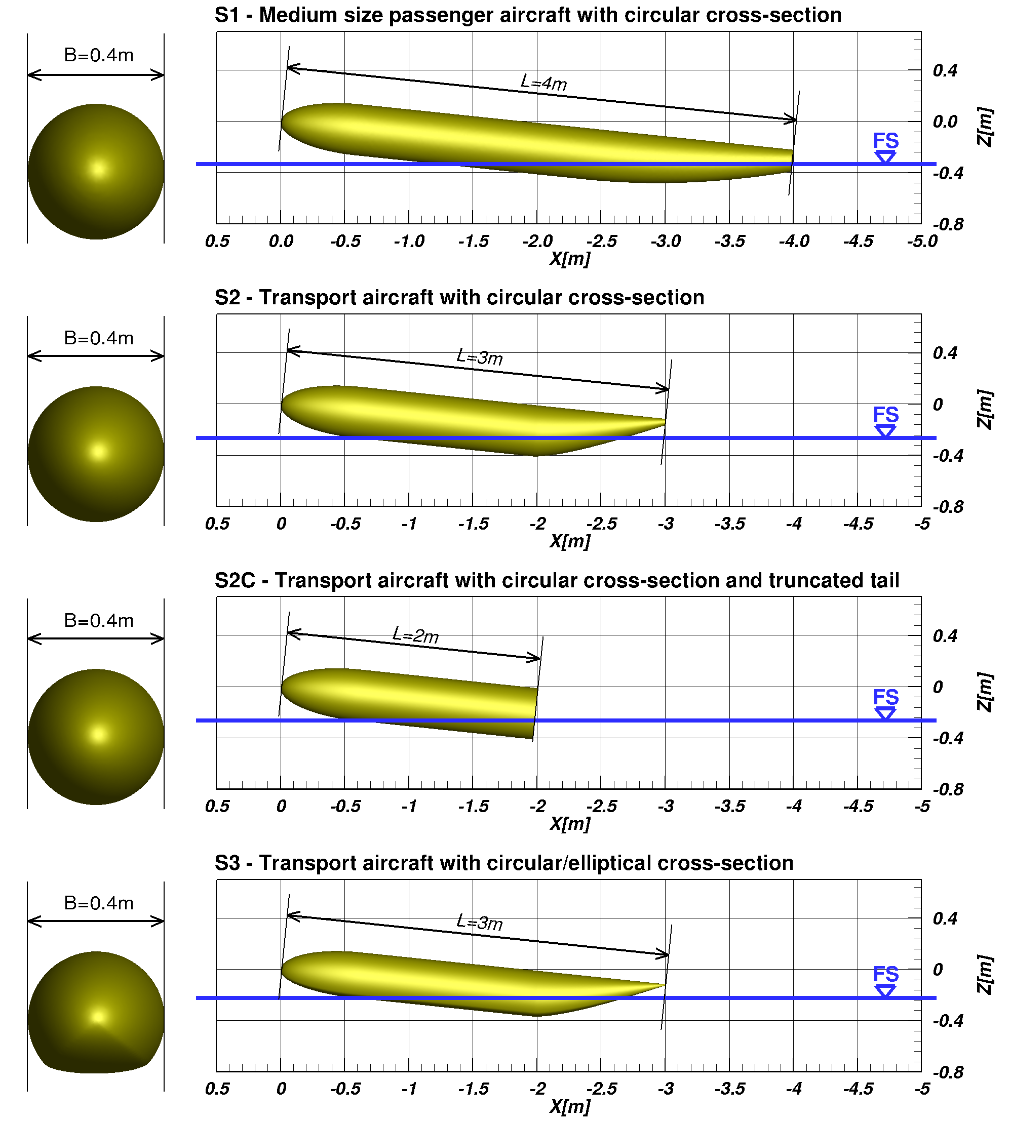
Figure 1: Fuselage shapes: side view (right column) and front view (left column).

The fuselage shape S1 resembles that of a small size passenger aircraft with a circular cross section, whereas the shapes S2 and S3 have a longitudinal profile similar to that of a freight transport aircraft, S2 being characterized by a circular cross section and S3 by a circular-elliptical cross section. Such a choice allows to investigate separately the effects of the longitudinal and transverse curvatures on the hydrodynamics and on the induced loads. Behind the nose region the fuselages display a cylindrical shape with a constant cross section. At the rear, the cross-section shrinks and moves up, leading to a bottom profile that varies rather smoothly in the shape S1 and more abruptly in the shapes S2 and S3. All the fuselage models have a breadth of 0.4 m, whereas the overall length varies between 3 m (S2 and S3) and 4 m (S1). In the fuselages S2 and S3 the cross section start shrinking from a distance of 2 m behind the fuselage nose (going from left to right) whereas in the fuselage S1 from a distance of 2.4 m. At those points a change in the longitudinal curvature occurs. In the case of the fuselage shape S1 the shrinking of the cross-section is much smoother, resulting in a milder longitudinal curvature, see again Figure 1. As a further study, a more extreme change in the longitudinal curvature is investigated in shape S2C, which is truncated at a distance of 2 m behind the nose. As detailed below, experimental measurements of hydrodynamic loads are available for S1, S2 and S3, whereas S2C has been only simulated.

In the following, a body fixed frame of reference, with the origin located on the fuselage nose is considered (Figure 2). The coordinates are indicated with capital letters $X$, $Y$ and $Z$. The $Z$ axis is aligned with the gravity acceleration $\bf{g}$, but positive upwards, the $X$ axis is aligned with the velocity of the towing carriage, pointing ahead. The $Y$ axis completes a right-handed coordinate system. The $X$-$Z$ plane, also denoted as the mid-plane in the following, is parallel to the undisturbed free surface.

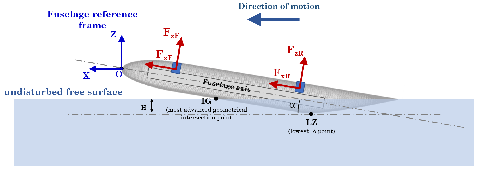
Figure 2: Reference frame used for the numerical data analysis and directions/signs of the forces recorded by the load cells.

The immersion depth of the fuselages $H$ is defined as the distance from the undisturbed free surface and LZ, i.e the point of the model at the lowest $Z$-coordinate at the specific pitch angle of the simulation, as shown in Figure 2. Instead, the most advanced geometrical intersection point between the lower longitudinal profile of the fuselage and the undisturbed water level is indicated by IG. Both these points are located in the mid-plane.

The numerical simulations are performed in deep fresh water conditions at a temperature of 16^∘, at which the density is $\rho=998.9$ kg/m³ and the kinematic viscosity is $\nu=1.107\times 10^{-6}$ m²/s. The fuselage advances at a speed of $U=5$ m/s with a fixed pitch angle of $6\degree$ and a nominal immersion depth of $H_{num}=146$ mm. The reference length and velocity to define the non-dimensional quantities and numbers are the length of the fuselages S2 and S3, i.e. $L=3$ m and the towing speed $U$, respectively. The corresponding Reynolds and Froude numbers are $Re=UL/\nu=1.355\cdot 10^{7}$ and $Fr=U/\sqrt{gL}=0.922$, since the acceleration of gravity is assumed to be $g=9.81$m/s². It is worth noting that during the corresponding experiments the actual immersion depth is different due to the lowering of the free surface associated to the aerodynamic effect of the carriage, as explained in Section 4.

3 Numerical Setup

3.1 Mathematical and Numerical Models

The numerical simulations are conducted by means of the in-house developed $\chi$navis code, solving the URANS equations. The solver is based on a finite volume discretization of the conservative equations for an incompressible viscous flows, which read as:

$${{\bf\Lambda}\frac{\partial}{\partial t}\int_{\mathcal{V}}{\mbox{\boldmath$q$}}{\rm\,\,d}V+\int_{\mathcal{A}(\mathcal{V})}[\Phi^{c}(\mbox{\boldmath$q$})-\Phi^{d}(\mbox{\boldmath$q$})]{\rm\,\,d}S={\bf 0}},$$ (1)

having denoted with $\mathcal{V}$ a control volume and with $\mathcal{A}(\mathcal{V})$ its the boundary. ${\rm\,\,d}S$ and ${\rm\,\,d}V$ are the infinitesimal volume and surface element, respectively. In this formulation all the variables are expressed in their non-dimensional form. In Equation 1, $t$ is the time, $x_{i}$ is the i-th space coordinate, ${\bf\Lambda}$$=$$\mbox{diag}\left(0,1,1,1\right)$ is a diagonal matrix, and $\mbox{\boldmath$q$}=(p,u_{1},u_{2},u_{3})^{T}$ is the vector of the non-dimensional variables for incompressible flows, which are the velocity components $u_{i}$ along the three directions and the hydrodynamic pressure $p$, which is related to the fluid pressure $\hat{p}$ and the acceleration of gravity $\bf g$ by $p$$=\hat{p}$$+(z-z_{FS})/Fr^{2}$, being $z_{FS}$ the (undisturbed) free surface level. It is worth noting that in the following the hydrodynamic pressure $p$ is the one used in the data analysis and in the graphs. $\Phi^{c}$ and $\Phi^{d}$ are the convective and viscous fluxes, i.e. $\Phi^{c}=[u_{i}n_{i};u_{j}u_{i}n_{i}+pn_{j}]^{T}$ and $\Phi^{d}=\left(0;\tau_{ji}n_{i}\right)^{T}$, where $i,j=1,2,3$. $n_{i}$ is the $i$-th component of the outward unit vector normal to the surface $\mathcal{A}(\mathcal{V})$ and $\tau_{ij}=\left(\nu_{t}+1/Re\right)\left({\partial u_{i}}/{\partial x_{j}}+{\partial u_{j}}/{\partial x_{i}}\right)$ are the components of the stress tensor. Finally, $\nu_{t}$ is the turbulent viscosity, which is modelled via the Spalart and Allmaras (1994) model.

The problem is closed by enforcing appropriate conditions at physical and computational boundaries. On solid walls, the relative velocity is set to zero (whereas no condition on the pressure is required). At the (fictitious) inflow boundary, the velocity is set to the undisturbed flow value, and the pressure is extrapolated from inside. On the contrary, the pressure is set to zero at the outflow, whereas velocity is extrapolated from the inner points. At the inlet, outlet and symmetry boundaries the extrapolation of pressure and velocity is obtained using a second order accurate approximation of their normal derivatives. For the conformal adjacent blocks, no interpolation is used; the values in the adjacent blocks are simply stored in a double layer of ghost cells. As for the overlapping grids, a tri-linear interpolation is used.

At the free surface, whose location is one of the unknowns of the problem, the continuity of stresses across the surface is required. If the presence of the air is neglected, the dynamic boundary condition reads:

$$\begin{array}[]{l}\displaystyle{p={\tau_{ij}}{n_{i}}{n_{j}}+\frac{z-z_{FS}}{{\mbox{Fr}^{2}}}}\\[5.69054pt] {\tau_{ij}}{n_{i}}t_{j}^{1}=0\\[5.69054pt] {\tau_{ij}}{n_{i}}t_{j}^{2}=0\end{array}$$ (2)

where $n$, $t^{1}$ and $t^{2}$ are the surface normal and the two tangential unit vectors, respectively. Surface tension effects are not taken into account.

The free surface, which has equation $\eta(x,y,z,t)=0$, is computed from the kinematic condition:

$$\frac{D\eta(x,y,z,t)}{Dt}=0$$ (3)

Initial conditions have to be specified for the velocity field and for the free surface:

$$\begin{array}[]{l}{u_{i}}\left({x,y,z,0}\right)=u_{i}^{0}(x,y,z)\quad i=1,2,3\\ \eta(x,y,z,0)={\eta^{0}}(x,y,z)\end{array}$$ (4)

The numerical solution of Equation 1 is obtained on a computational domain discretized by adjacent or overlapped structured blocks composed of hexahedral volumes. A suitable overlapping grids approach is exploited to handle either complex geometries or multiple bodies in relative motion (see Zaghi et al. (2015)). Conservation laws are enforced in each control volume in an integral form. The surface integrals are evaluated by means of a second-order formula. For the viscous fluxes, the velocity gradients are computed using a standard second-order centred finite volume approximation. Numerical convective fluxes are computed solving a Riemann problem whose left and right states are estimated by means of a third-order upwind-biased scheme (Van Leer, 1979). A second-order accurate solution of the Riemann problem is derived, which reduces the computational cost necessary to compute iteratively the exact one (see Posa and Broglia 2019 for more details). Time integration is performed by a second-order three-points implicit backward finite-difference scheme. The resulting system of coupled non-linear algebraic equations is tackled via a pseudo-time technique (Chorin (1967)), using an implicit Euler scheme with an approximate factorization (Beam and Warming 1978). A local dual time step and a multi-grid technique are exploited for faster convergence in the pseudo-time.

Free surface effects are taken into account by a single phase level-set algorithm (Di Mascio et al., 2007), (Broglia and Durante, 2018). The resulting scheme is globally second-order accurate in both space and time, producing oscillation-free solutions, also in presence of discontinuities (see, for example, Di Mascio et al. (2009)).

3.2 Fluid Domain and Computational Grid

Taking advantage of the symmetry of the flow with respect to the mid-plane $X-Z$, only half of the domain is considered. In the $X$-direction the domain extends $1.5L$ upstream and $4L$ downstream of the fuselage nose, i.e. the computational domain is $5.5L$ long. In the $Y$-direction it extends from the symmetry plane to $Y=2L$, whereas in the $Z$-direction from $0.2L$ above the fuselage nose to $2L$ below it.

The boundary conditions are summarized in (Figure 3) . Symmetry boundary conditions are imposed on the $Y=0$ plane. It is worth noting that, even if the top boundary is placed only at $Z=0.2L$ above the fuselage nose, the air flow is not simulated, thus this circumstance does not affect the validity of the simulations. At this boundary all the variables are simply extrapolated.

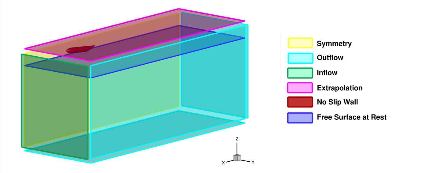
Figure 3: Computational domain and boundary conditions.

  

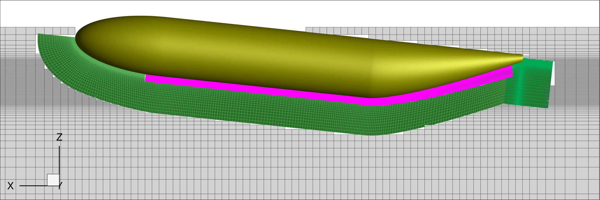
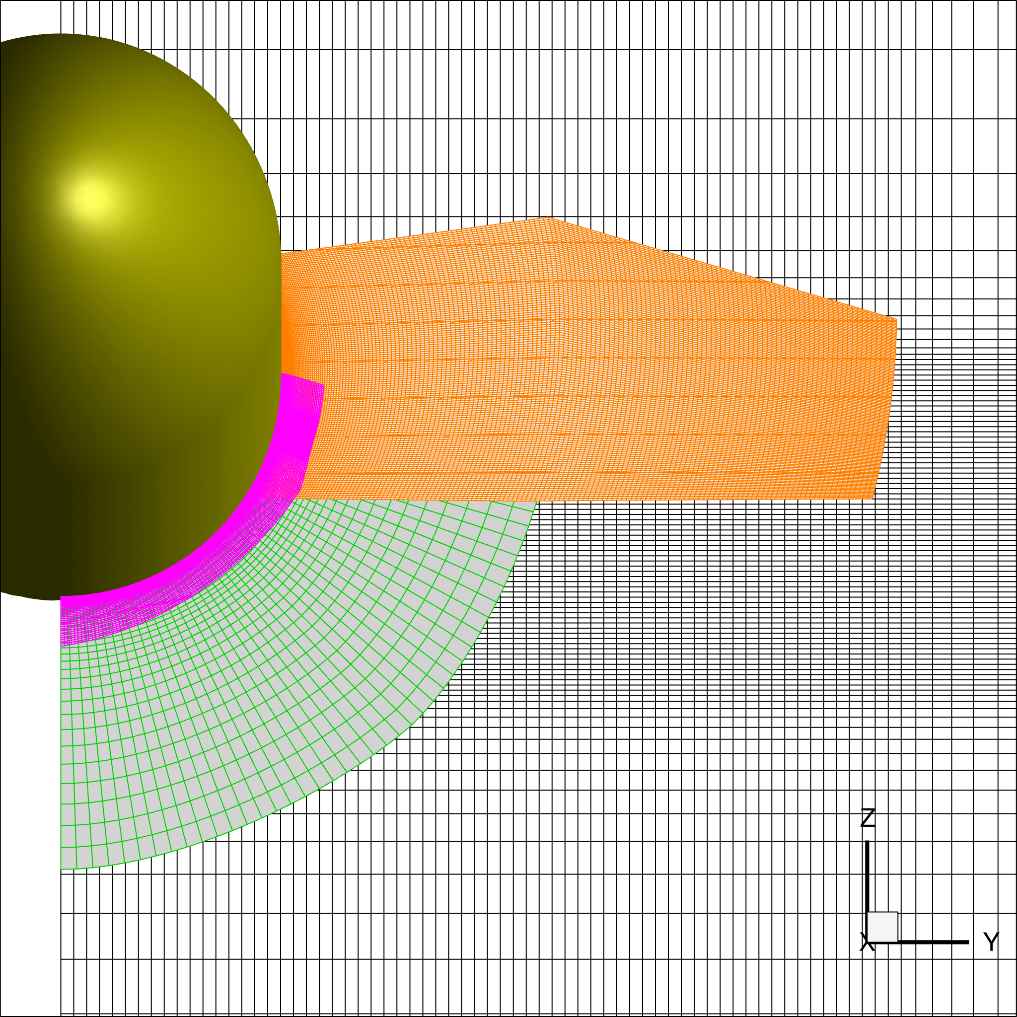
Figure 4: Details of the computational mesh.

The computational mesh is a structured grid composed of adjacent and overlapping blocks. As shown in the detailed views shown in Figure 4, the near wake region (in green) is further refined (in purple) to capture accurately the formation of the spray root. A refined region is also considered farther away from the wall (in orange) to capture the plunging of the spray detaching from the fuselage on the free surface.

The height of the first cells of the mesh on the surface is set in order to achieve an average wall normal spacing below 1 viscous unit. The outer part of the domain is discretized by a Cartesian background mesh. A similar grid topology is adopted for the different test cases, whereas the block distribution and grid spacing are tailored for the specific case. The total number of discretization volumes depends on the test case, and counts up to about 15 millions of control volumes.

The numerical solutions are computed on four grid levels, generated by removing every other grid points from the next finer one. In the grid sequencing procedure, the solution is first computed on the coarsest grid level, then, it is prolonged onto the next finer grid. On the finer meshes, the multi-grid algorithm accelerates the convergence in the pseudo-time using all the available coarser grid levels. A physical non-dimensional time step equal to $5\times 10^{-3}$ is used for the time integration on the finest mesh, while on coarser mesh the time step is multiplied by a factor 2.

The computational problem is tackled here via parallel High Performance Computing, distributing the structured blocks among all available CPUs. Communications across them for the coarse grain (distributed memory) parallelization is achieved via calls to standard Message Passing Interface (MPI) libraries, whereas for fine grain (shared memory) parallelization is based on Open Message Passing (OpenMP) libraries.

4 Experimental setup

The experiments are carried out in the CNR-INM Wave Tank. The towing carriage is operated at a speed of 5 m/s, with a maximum fluctuation of about 0.15 %.

The tests are carried out in calm water and at fixed attitude (captive tests), i.e. at a fixed pitch angle $\alpha=6^{\circ}$ and immersion depth $H_{exp}$=150 mm.

The attitude regulation is performed through a 2-degree-of-freedom system driven by two linear servo-actuators. The instrumented fuselage model S3, installed on the carriage is shown in Figure 5.

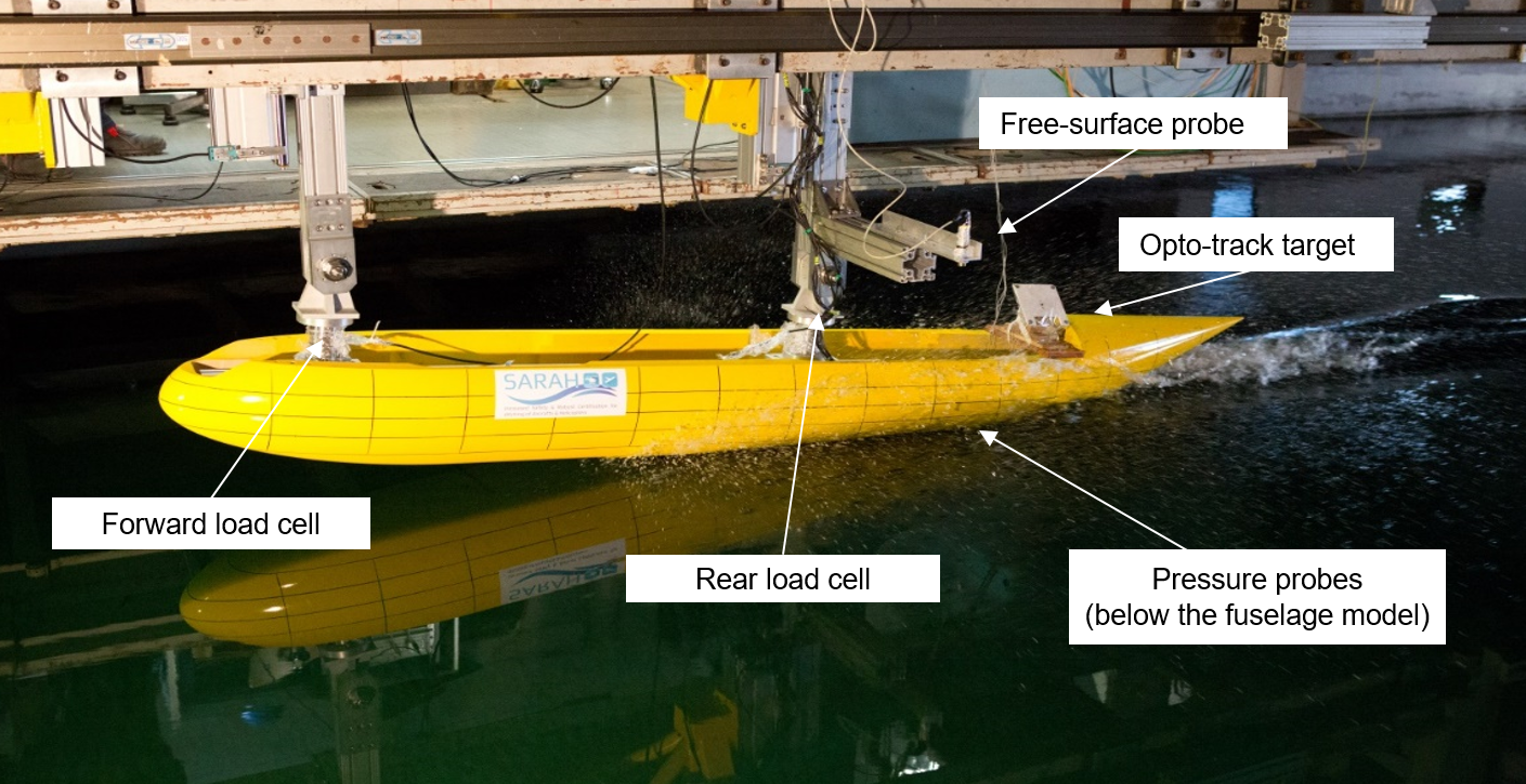
Figure 5: Picture of the instrumented fuselage model S3.

The free surface probe located at the rear of the fuselage is used for the positioning of the fuselage with respect to the undisturbed water level before each run. The opto-track system is employed as a cross-check of the free surface probe measurements. Thanks to the combined use of these devices, the final position can be considered quite accurate, with an uncertainty of $\pm$1 mm. The connection of the fuselage models to the actuator system is achieved by means of two 6-axes piezoelectric load cells. The load directions and signs are shown in Figure 2. The forces $F_{xF}$ and $F_{xR}$, referring to the front and rear load cells respectively, are parallel to the fuselage axis, whereas $F_{zF}$ and $F_{zR}$ are normal to the fuselage axis in the vertical plane.

For their operational principle, the load cell readings are zeroed before any acquisition. The zeroing is performed over a short time interval (about 1 s) when the fuselage models are already submerged in water at the required attitude. In this position the forces acting on the fuselage are the weight and the hydrostatic buoyancy.

Although this type of captive tests guarantees a very precise control of the attitude and of the immersion depth of the model, they are characterised by some drawbacks that have to be accounted for. First of all the, the towing carriage in use is located very close to the water surface of the basin. This creates an unavoidable aerodynamic effect, for which the water level below the carriage during the run is slightly different than that at rest. Through some specific measurements of the free surface level performed without the model installed, it is found that the free surface lowering at a carriage speed of 5 m/s is about 4 mm. This is the reason why, to facilitate the comparison of the results, the numerical simulations are performed at $H_{num}$=146 mm. Secondly, after each run some residual waves remain, which are characterized by a very low decay rate. Even after thirty minutes, a standing wave with a period of 70 s and amplitude of about 3 mm is observed. The only way to remove the effects of the residual standing wave on the force measurements is to perform averages over sufficiently long time intervals.

Finally, it is worth noting that while the present present simulations are performed at fixed attitude, in the aircraft ditching case the vertical and horizontal velocities are the results of the combined effects of the hydrodynamic loads, the aerodynamic loads, determined by the aircraft wings and control surfaces, and by the action of the engines. As such, the actual loads may differ from what found in the present simulations.

5 Results

The flow field characteristics are first described in details for the fuselage shape S2. In order to explain more deeply the physical origin of the suction area at the rear, where the longitudinal curvature change occurs, the surface pressure field of S2 is compared with that of S2C, i.e. the truncated fuselage model. Hence, the effects of the fuselage shape in terms of pressure and free surface shape at the spray root and at the rear are analysed. Successively, the overall forces $F_{X}$ and $F_{Z}$ acting on the fuselage models, as well as their longitudinal distributions are derived. The forces are investigated by decomposing them into three contributions: the viscous, the buoyancy and the hydrodynamic ones. The forces computed by the numerical simulations are finally compared with the experimental measurements for the purpose of validation.

5.1 Spray evolution and wave pattern

An overview of the free surface shape around the fuselage and of the pressure coefficient, defined as $C_{p}\doteq 2p$, on the wall is shown in Figure 6, where, for the sake of clearness, the solution is mirrored a the longitudinal plane of symmetry. The wave pattern shown in this figure is that of the S2 shape, advancing at $U=5$ m/s, with 6^∘ pitch angle and an immersion depth of 146 mm.

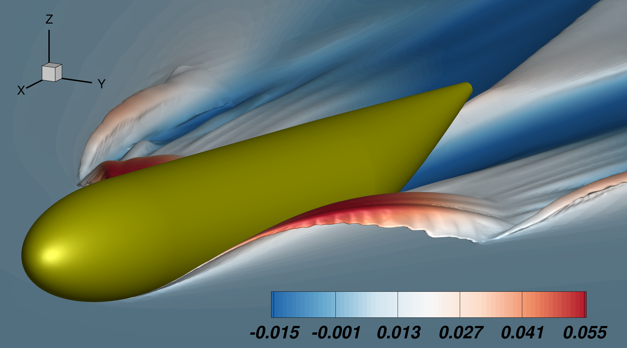
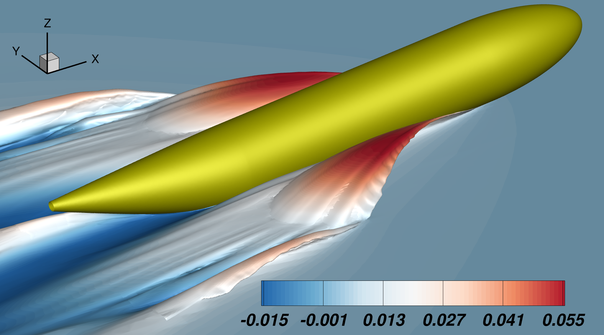
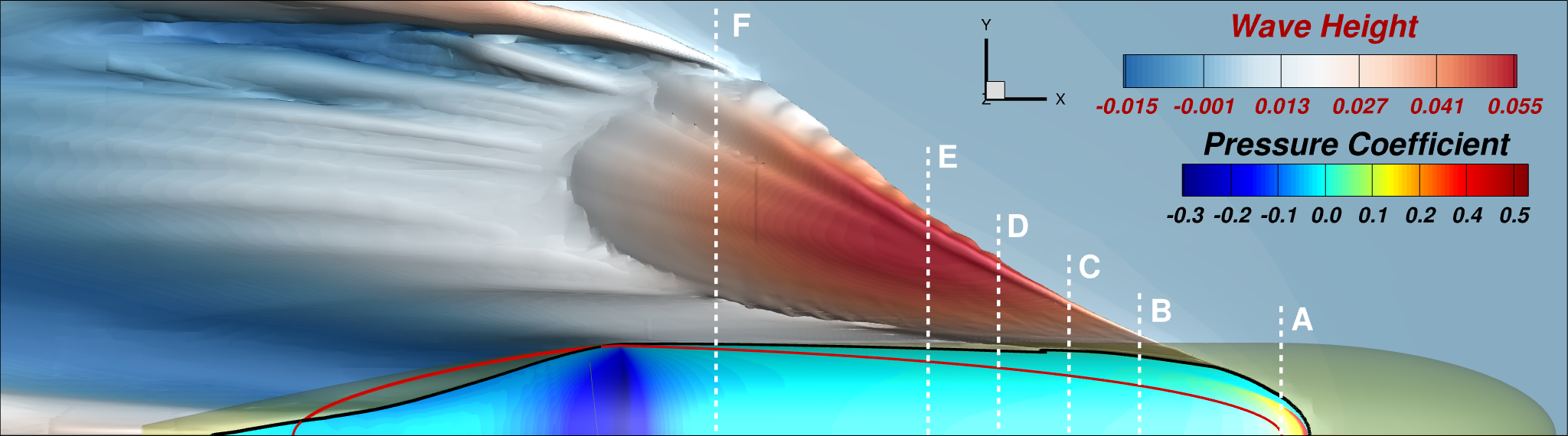
Figure 6: Free surface derived from the numerical simulation of the fuselage model S2, view from the front and from the back (top) and view from above (bottom). In the bottom figure the pressure coefficient $C_{p}$ on the wetted area is also shown. Dashed lines and capital bold letters refer to the cross sections shown in the following.

The main features of the flow field resemble those of planning hulls (see for example Broglia and Durante (2018)). Differently from the displacement vessels case at low Froude numbers, in which a classical Kelvin wave system forms immediately around the hull, in this case a spray is formed beneath the fuselage. The spray leaves the fuselage and plunges onto the free surface, leading to a rather complex flow behind. Due to the high pressure occurring in the front part of the fuselage (see the panel at the bottom of Figure 6), this spray rises up both ahead and laterally.

The free-surface shape generated by the fuselage can also be investigated by means of a 2D+$t$ approach e.g. Iafrati and Broglia (2008); Broglia and Iafrati (2010). By doing so, the steady flow can be approximated as a water entry problem in the transverse plane, on an earth fixed reference frame. From this point of view, the spray remains attached to the body in an early stage but detaches from the body afterwards, e.g. Sun and Faltinsen (2006).

This process is shown in more detail in Figure 7, where the pressure coefficient variation and the evolution of the free surface are shown at different cross-sections in the longitudinal direction.

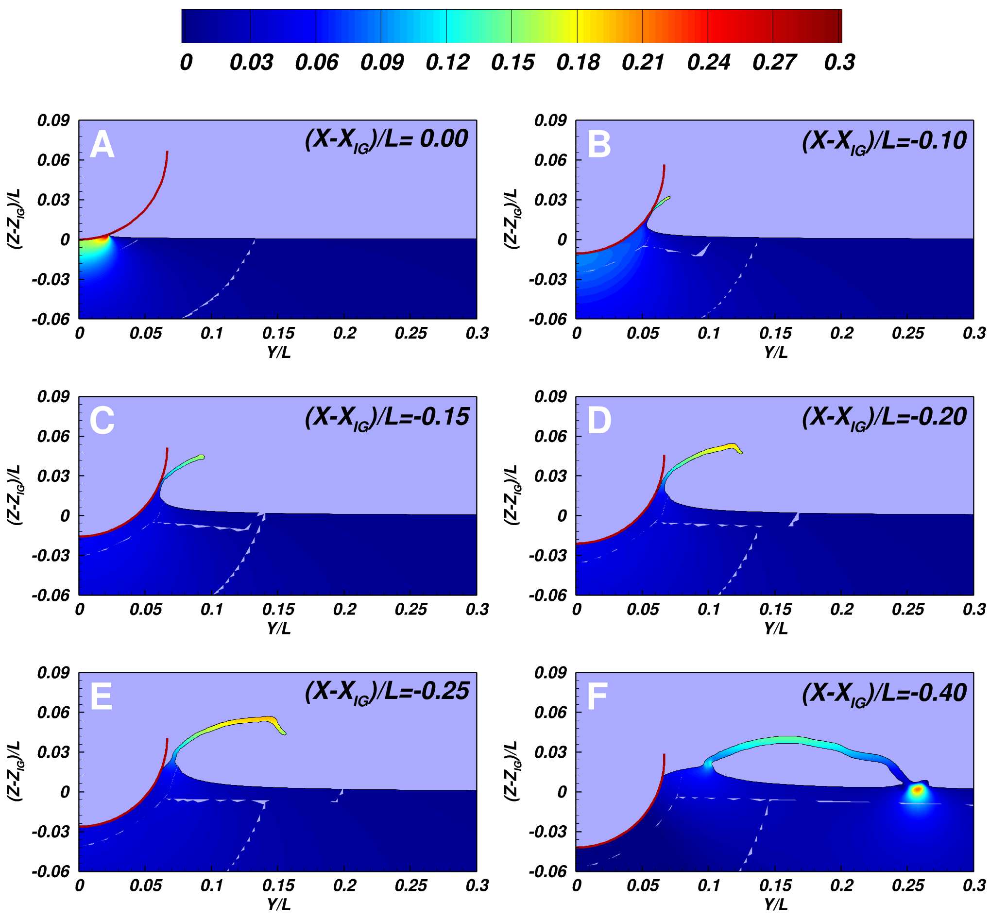
Figure 7: Free surface shape evolution along the $X$-axis of the fuselage S2, coloured with the contour maps of the hydrodynamic pressure coefficient $C_{p}$. The red solid line represents the edge of the fuselage cross section at each specific $X$-location.

For convenience, the position of these cross-sections is relative to $X_{IG}$, the abscissa of IG. Their positions are indicated with white dashed lines in Figure 6. In the first cross-section (top-left) the pressure peak at the spray root and the water rise can be noted. The jet separation and its lateral evolution appear in the following two cross-sections. Moving backwards, the spray detaches at about $(X-X_{IG})/L=-0.10$ and starts to plunge at $(X-X_{IG})/L=-0.25$. At $(X-X_{IG})/L=-0.40$ it falls onto the free surface, thus leading to a high pressure pulse. As a consequence, see Figure 6, a large spray sheet, hydraulic bores and ricochets form in the wave pattern. A strong interaction among these structures is observed, resulting in a very complex free surface shape in that region.

The lowering of the free-surface observed at the rear of the fuselage (evident in the bottom panel of Figure 6), is a consequence of the low hydrodynamic pressure region generated by the change in the longitudinal curvature that induces an increase in the fluid velocity.

Finally, behind the fuselage the accelerated flow leaves the body surface tangentially, leading to the formation of the typical rooster tail shape, similar to that observed in high speed crafts.

5.2 Hydrodynamic pressure on the fuselage

The contour maps of the hydrodynamic pressure coefficient over the wetted surface are shown in the bottom panel of Figure 6 and in Figure 8.

In the spray root region, just like in planing hulls or in flat plates moving in water at high speeds (Faltinsen (2005), Savitsky (1964), Iafrati (2016), Broglia and Durante (2018)) a region of maximum pressure is observed. In this context flow separation refers to the detachment of the free surface from a solid wall. Accordingly, the separation line is the contact line between them. The separation line from the fuselage wall in motion is shown in the bottom panel of Figure 6 with a black line, whereas the red thick line indicates the geometrical intersection line between the fuselage and the undisturbed free surface. The separation line is located outside the geometrical intersection line, this implying a a water pile-up, and the distance between these lines increases while moving backwards along the $X$-direction up to a certain point. Going backwards, the separation line gets closer the geometrical intersection line, until they meet at about $X=X_{LZ}$. Behind LZ, due to the acceleration of the fluid and the lowering of the free-surface, the separation line is located inside the geometrical intersection line, see again Figure 6.

It is worth noticing that the flow accelerates just ahead of the curvature change ad decelerates behind it, i.e. moving from left to right in Figure 8. This circumstance is associated with a pressure drop to negative pressure values ahead the curvature change, followed by a pressure recovery behind. This situation can also be interpreted from a 2D+$t$ perspective (Iafrati and Broglia (2008), Broglia and Iafrati (2010)). From this point of view, the longitudinal curvature of the fuselage introduces a variation in the vertical entry velocity $V_{b}$ of the body contour in an earth-fixed transverse plane, which can be written as $V_{b}=V\sin\theta$, where $\theta$ is the local inclination angle of the bottom profile in the longitudinal plane. In the front part $\theta$ is constant and positive, and so is the vertical entry velocity. However, starting from the curvature change and going backwards, $\theta$ decreases and becomes progressively negative, thus turning the problem from a water-entry to a water-exit one. As shown in Del Buono et al. (2021), this causes the shrinking of the wetted surface and the generation of negative pressure and suction loads.

5.3 Comparison between the full and the truncated fuselage flows

As mentioned above, in order to improve the understanding of the mechanism of pressure decrease at the curvature change at the rear, it is very informative to compare the simulation of the full fuselage shape S2 with that of the truncated fuselage S2C, shown in Figure 1, at the same conditions. A comparison between the $C_{p}$ contour lines in the mid-plane for S2C and S2, as well as between the $C_{p}$ contour maps on the wall, is shown in Figure 8.

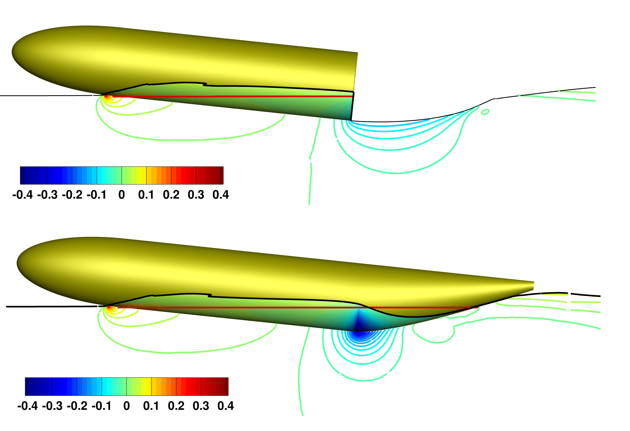
Figure 8: $C_{p}$ contour lines for the truncated fuselage S2C (top) and for the full fuselage S2 (bottom) on the midplane $X-Z$ and $C_{p}$ colour contour maps over the wetted surfaces.

As expected, the pressure fields in the front part present a very similar trend. Instead, the $C_{p}$ pattern at the stern of S2C resembles that of the dry-transom flow, typical of planing hulls, in which the free surface separation from the body occurs exactly at LZ, i.e. at the transom, (see for example Broglia and Durante (2018); Iafrati and Broglia (2008); Broglia and Iafrati (2010)), which remains completely dry, with a hydraulic jump behind it. The flow accelerates in the rear part of the truncated fuselage, causing a weak pressure drop. However, this pressure drop is much lower with respect to the full fuselage case, since for the truncated case at LZ the global pressure is forced to be almost null, due to the boundary condition at the free surface, see Equation 2. On the other hand, as it is shown in Figure 8, for the full fuselage shape S2, the free surface remains attached to the wall also behind LZ, and a more intense flow acceleration results, leading to the situation described in Section 5.1 and Section 5.2.

5.4 Effect of the fuselage shape

In order to investigate the effects of the different fuselage shapes on the hydrodynamics, the $C_{p}$ contour maps over the wetted surface of S1, S2 and S3 are compared in Figure 9. In particular, the front part is shown on the left side, whereas the rear part is shown on the right side. For convenience, in the left-side plots the fuselages are aligned with respect to IG, whereas in the right-side plots they are aligned with respect to LZ (see Figure 2 for their definitions).

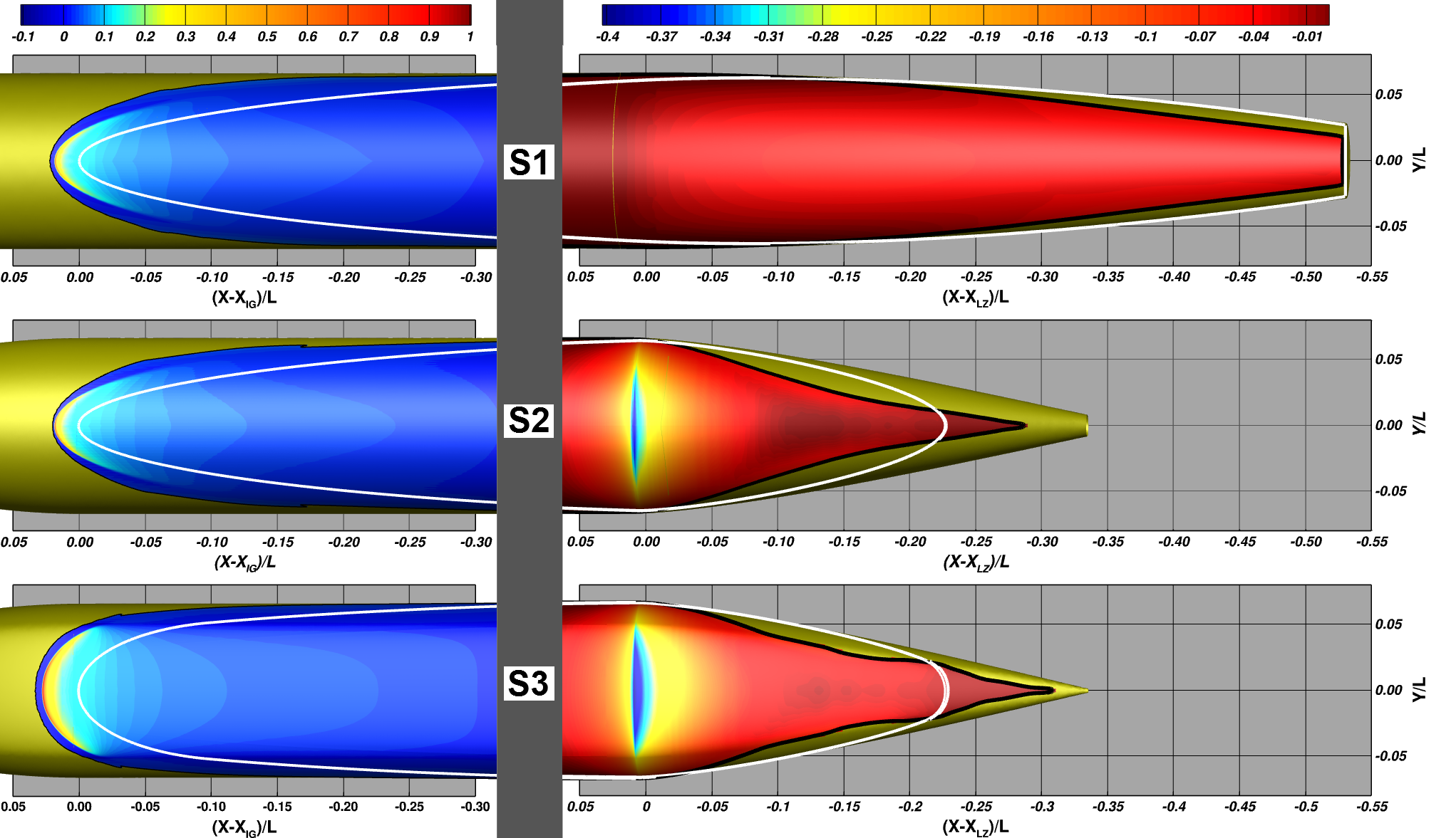
Figure 9: $C_{p}$ contour maps for the three fuselage shapes S1 (top), S2 (middle) and S3 (bottom), at the spray root (left) and in the region of longitudinal curvature change (right). The black and white solid lines identify the separation lines in motion and the geometrical intersection line with the undisturbed free surface, respectively.

The black and the white solid lines identify the separation line and the geometrical intersection line with the undisturbed free surface respectively. It is worth reminding that S1 and S2 have a circular cross section from the end of the nose up to the point of longitudinal curvature change. The lower part of the cross section of S3 is elliptical and “flatter” than S2. The longitudinal curvature change at the rear is smooth in S1, whereas it is quite abrupt for the shapes S2 and S3.

As already observed in Section 5.1, the water impingement on the fuselage body at the front leads to a high pressure region, which on its turn induces a water pile-up and a spray, clearly displayed in all the fuselages. As expected, the pressure trends and values, as well as the separation lines, for the fuselages S1 and S2 are very similar in shape. The pressure in S2 appears slightly lower than in S1. This is due to the fact that the spray root in S2 lies at the end of the nose region, whereas in S1 is in the region of constant longitudinal curvature, see Figure 1. There are much more significant differences between the pressure trends of S1/S2 and that of S3, mainly as a results of the flatter shape, and thus of the generally lower deadrise angle. For this reason the pressure peak in the shape S3 on the midline is higher than in the shapes S1 and S2, and so are the pressure values at the sides in the spray root region. It is also observed that in S3 the distance between the spray root and the spray tip (which is approximately the distance from the location of maximum pressure to the separation line) is larger than in S1 and S2 and is rather uniform moving from the midline to the sides.

In order to better visualise the effect of the transverse shape on the flow field, the $C_{p}$ contours and the free surface shapes in the mid-plane (i.e. $Y/L=0$) are shown in Figure 10.

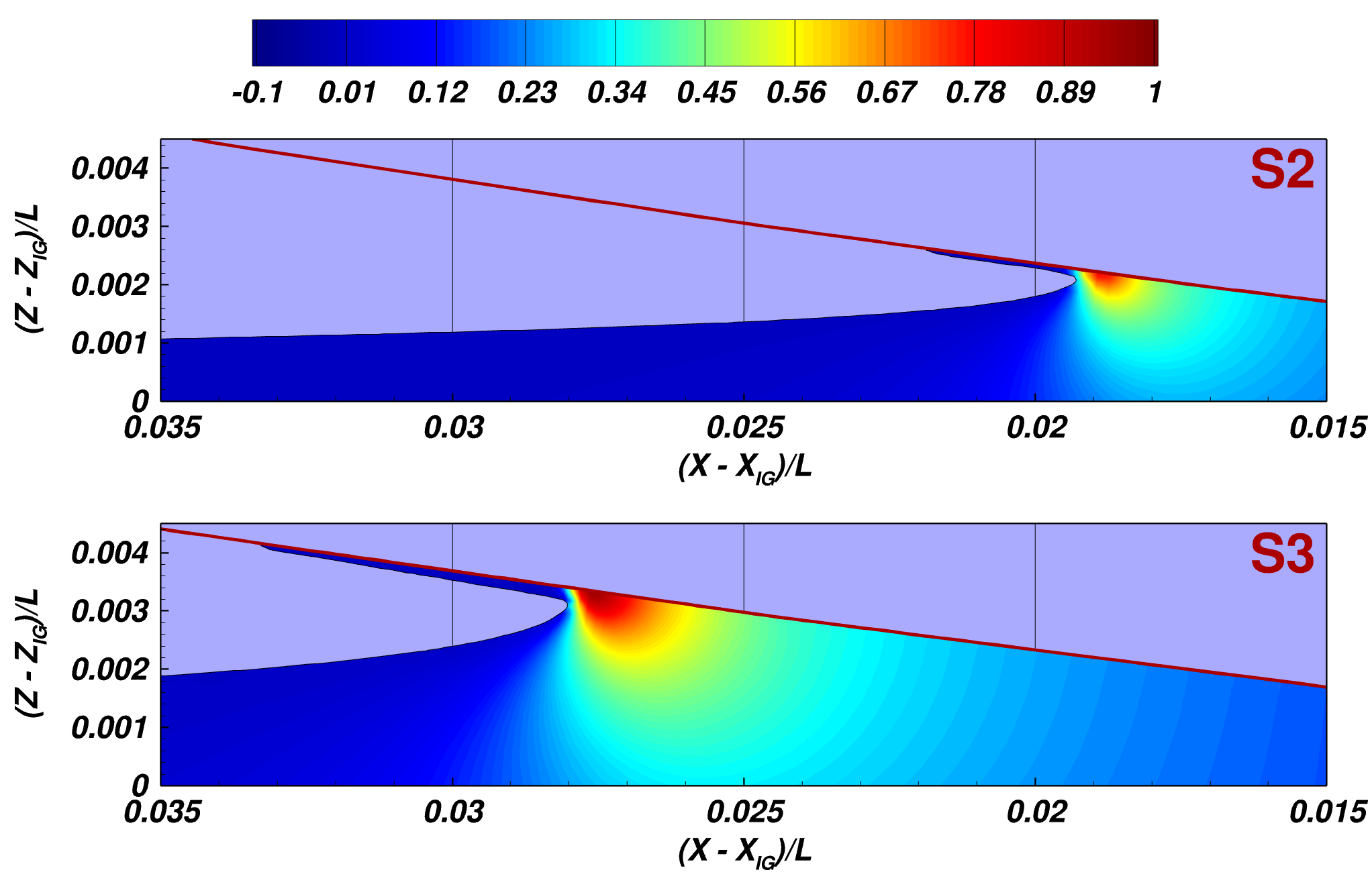
Figure 10: $C_{p}$ contours for the S2 and S3 fuselage shapes in the mid-plane delimited by the free surface. The red solid line represents the edge of the fuselage mid-plane section.

In these plots only the results for S2 and S3 are shown, being the data for S1 very similar to those of S2. For convenience, the reference point for the comparison is the $X$-coordinate of IG. In Figure 10 the water pile-up in front of the geometrical intersection point IG is visible for both shapes, with the thin water spray remaining well attached to the body surface. As expected, the maximum pressure occurs approximately just behind the spray root, with the pressure peak recorded for shape S3 being higher than that for S2. As a consequence, the spray extends slightly further ahead, and the water pile-up is more relevant in S3. These effects are again related to the flatter lower surface and to the reduced possibility of the fluid to escape from the sides.

The evolution of the spray is also strongly affected by the fuselage shape, as shown in Figure 11, where the $C_{p}$ contours and the free surface shape are plotted on several cross-sections along the longitudinal direction.

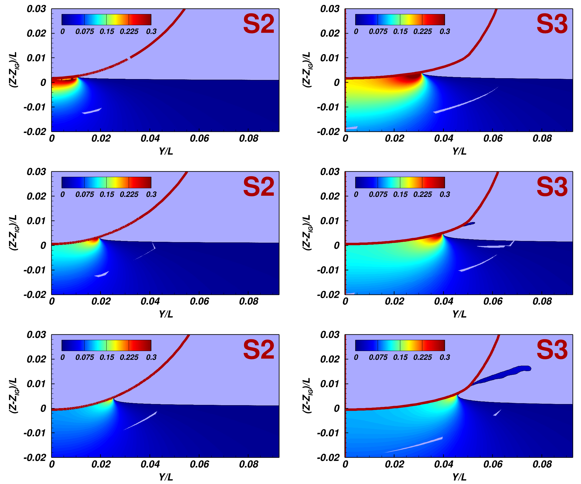
Figure 11: Free surface at different longitudinal sections for the shapes S2 and S3: $(X-X_{\textrm{IG}})/L=0.015$ (top) $(X-X_{\textrm{IG}})/L=0.005$ (middle) and $(X-X_{\textrm{IG}})/L=-0.005$ (bottom), coloured with the contour maps of the hydrodynamic pressure coefficient $C_{p}$. The red solid line represents the edge of the fuselage cross section at each specific $X$-location.

At $(X-X_{\textrm{IG}})/L=0.015$, i.e. ahead of IG the free surface is still attached to the body for both shapes. As already anticipated, due to the smaller deadrise angle, the maximum pressure values for S3 are higher then those for S2. Moving backwards, i.e at $(X-X_{IG})/L=0.005$, the spray tip in S3 reaches the point where the transverse shape profile changes from elliptical to circular, see Iafrati et al. (2020). The sudden change in the transverse curvature facilitates the detachment of the spray from the body surface. Further downstream, the water spray freely evolves under the effect of gravity. Due to the more uniform curvature, in the S2 the separation of the water spray from the wall takes place further downstream, as shown in Figure 7.

The analysis of the flow field at the rear is more complex. A comparison between the $C_{p}$ contour maps in that region is shown in the right column of Figure 9. It is evident that in all cases, as a results of the change in the longitudinal curvature, the flow accelerates ahead of LZ, hence the pressure decreases down to negative values, and re-accelerates behind LZ, leading to a pressure increase. For the fuselage S1 the pressure reduction is very mild and extends for a large distance behind LZ. On the contrary, in the fuselages S2 and S3, as a results of the abrupt curvature change, the flow acceleration and deceleration ahead and behind LZ respectively are much relevant, producing a significant and much more localised negative pressure area, in which the $C_{p}$ reaches values of about -0.4. In S2 the area of negative pressure is smaller than in S3, both ahead and behind LZ, and especially at the sides. This is clearly an effect of the flatter bottom of the fuselage shape S3.

5.5 Forces acting on the fuselage

The forces acting on the fuselage are derived by integration of the pressure and of the wall shear stress fields over the wetted surface of the fuselages. Three different contributions are distinguished, namely the viscous contribution (${\bf F_{v})}$, the buoyancy contribution (${\bf F_{B}}$) and the pure hydrodynamic pressure contribution (${\bf F_{D}}$), derived as:

$$\begin{array}[]{l}\displaystyle{{\bf F_{v}}=\rho U^{2}L^{2}\int_{S}\tau\,{\bf n}\,dS}\\[8.53581pt] \displaystyle{{\bf F_{B}}=\rho U^{2}L^{2}\int_{S}\frac{z-z_{FS}}{Fr^{2}}\,{\bf n}\,dS}\\[8.53581pt] \displaystyle{{\bf F_{D}}=\rho U^{2}L^{2}\int_{S}p\,{\bf n}\,dS}\end{array}$$ (5)

In Equation 5, $\bf n$ is the normal (directed into the fluid) to the wetted surface $S$, $p$ is the non-dimensional hydrodynamic pressure and $\tau$ denotes the non-dimensional shear stress tensor. The analysis is performed for the in-plane forces (i.e. the projection along the $X$ and $Z$ axes of the different force contributions). It is worth noting that in this case the force and the force contributions are dimensional quantities (in N). The total force contributions for the four fuselages are reported in Table 1 and, graphically, in the bar plots of Figure 12.

Table 1: Total force contributions to $F_{X}$ and $F_{Z}$ for all the fuselage shapes. In the column “viscous” the flat plate analogy results are shown in round brackets.

	Shape	viscous	hydrodyn.	buoyancy	TOT
$F_{X}$ [N]	S1	-43.2 (-39.1)	-24.8	-1.5	-69.4
	S2	-33.4 (-30.0)	-27.6	-1.0	-61.9
	S2C	-25.9 (-22.4)	-16.9	-22.5	-65.3
	S3	-38.9 (-33.5)	-36.2	-3.7	-78.8
$F_{Z}$ [N]	S1	-0.8	-3.7	563.1	558.6
	S2	-0.5	-51.8	343.5	291.2
	S2C	-0.9	157.8	215.0	371.9
	S3	-1.2	-68.0	445.8	376.6

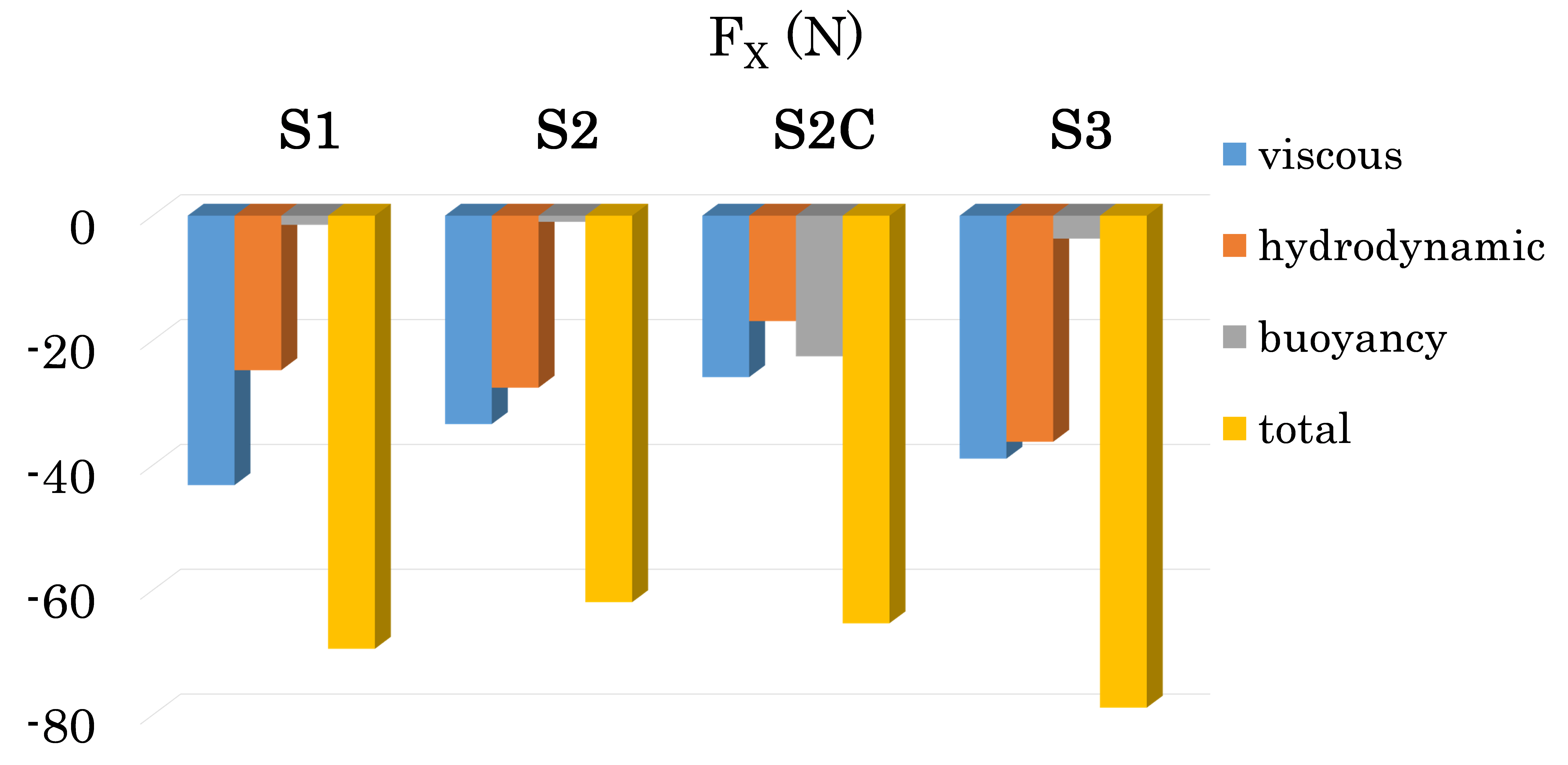
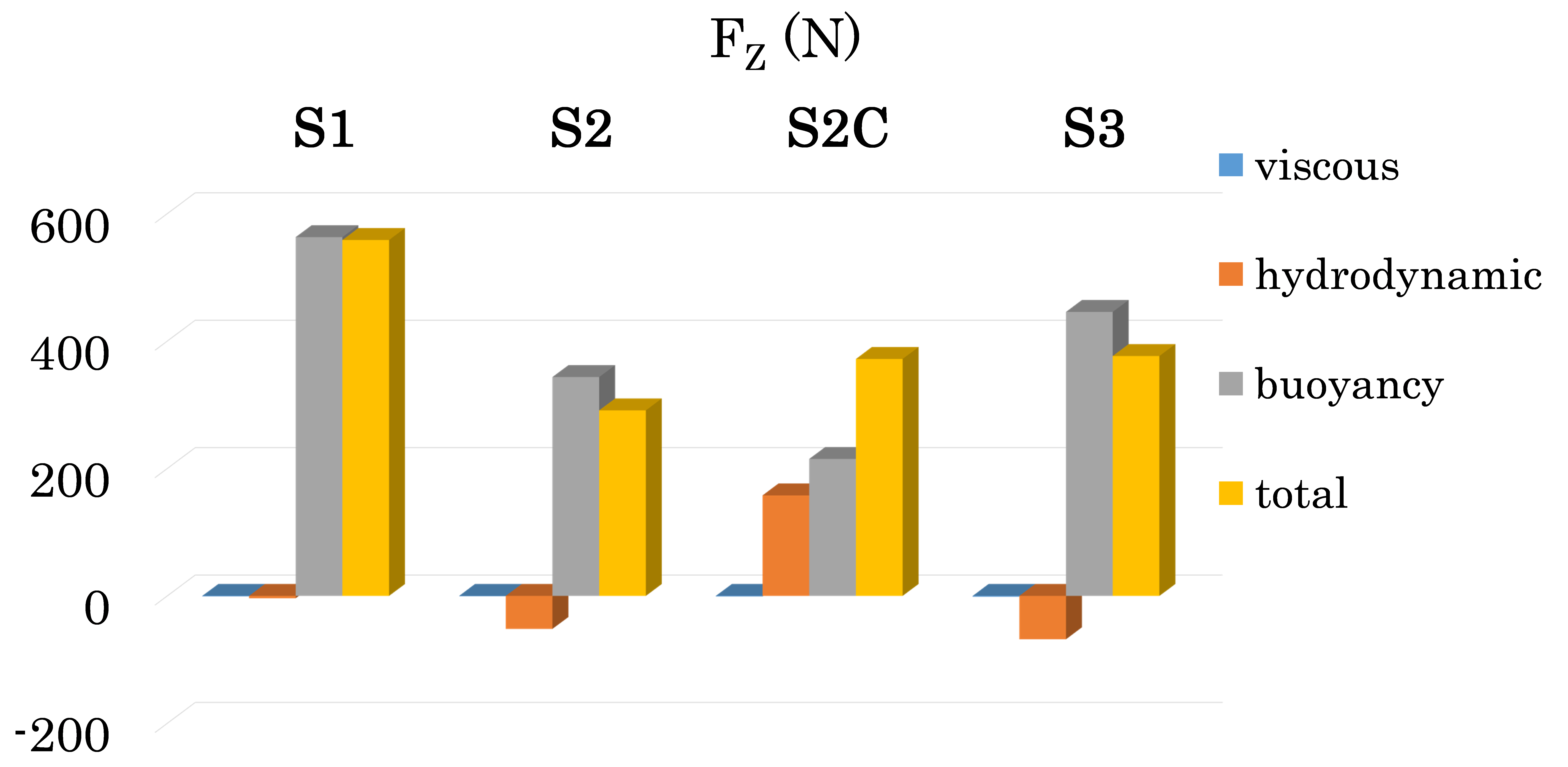
Figure 12: Histograms of the viscous, buoyancy and hydrodynamic contributions to $F_{X}$ (left) and $F_{Z}$ (right).

The viscous contribution in the $X$ direction for all the shapes is in a reasonably close agreement (although about 10% lower) with the skin friction resistance $R_{FP}$ obtained using a flat plate analogy, in which the skin friction coefficient $C_{FP}$ is estimated as a function of Re_L through the Hughes correlation, see Faltinsen (2005), and $R_{FP}=1/2\rho U^{2}C_{FP}S_{wet}$. The viscous and the hydrodynamic contribution to $F_{X}$ are of the same order of magnitude, whereas the buoyancy contribution is negligible in all cases, as expected. The ratio of the viscous contribution to the total value of $F_{X}$ spans from about 50% for the shapes S2 and S3 to 60% for the shape S1. This is a consequence of the larger wetted surface of S1 compared to the other shapes.

As far as the $Z$-components are concerned, at this Froude number the hydrodynamic contribution is negative in all cases, except for the truncated fuselage shape S2C. For the shape S1 the hydrodynamic contribution is very close to zero, whereas for shapes S2 and S3 is about -50 N and -70 N, respectively. In all cases, except for the shape S2C, the hydrodynamic contribution is much lower in amplitude than the buoyancy contribution, which is positive and largely predominant. Therefore the total force values result positive, i.e. oriented upwards.

5.5.1 Comparison with the experimental measurements

The loads acting on the fuselage derived from the numerical simulations are here validated against the measurements. A zeroing procedure similar to that followed during the experiments has been performed numerically, i.e. the hydrostatic loads, calculated at rest, are subtracted from those derived from the simulations of the fuselages in motion. The validation assessment is summarized in Table 2.

Table 2: Comparison between numerical and experimental loads.

	Shape	Numerical	Experimental	Uncertainty	Deviation
$F_{X}$ (N)	S1	-69.4	-71.3	4.0%	2.69%
	S2	-61.7	-68.2	4.0%	10.58%
	S2C	-65.2
	S3	-78.8	-83.3	4.0%	5.73%
$F_{Z}$ (N)	S1	-78.0	-48.2	22.0%	38.20%
	S2	-112.5	-106.9	22.0%	4.99%
	S2C	118.8
	S3	-123.1	-128.2	22.0%	4.15%

Having already compensated the water level lowering of 4 mm below the carriage during the run, the experimental uncertainty reported in Table 2 takes into account the effect of a residual basin standing wave of amplitude 3 mm. The residual standing wave affects both the zeroing process and the time averages. To evaluate the first source of uncertainty, the hydrostatic force acting on the S2 fuselage at different immersion depths, spanning a range of $\pm$ 6 mm about the nominal one, are computed. The effect of a different water level during the run can be evaluated by computing the forces acting on the fuselage in motion at $U=5$ m/s at different immersion depths, still spanning a range of $\pm$ 6 mm about the nominal one. The force trends in the examined range are found to be linear. Combining these analyses, an uncertainty of of 4 % and 22 % for the $X$ and the $Z$ force components respectively are estimated. These uncertainties are of the same order of magnitude of those estimated by analysing the acquired force time histories during the part of the carriage run at constant speed.

The percentage deviations between the experimental and numerical results, reported in the last columns of the Table 2, are computed as:

$$\textrm{Deviation}=100\cdot\frac{F^{exp}-F^{num}}{F^{num}}$$

where $F^{exp}$ is the measured force value and $F^{num}$ is the zeroed forces derived numerically. The comparison denotes a fairly good agreement between the CFD estimation and the experimental tests. The deviation for $F_{X}$ is of the same order of magnitude of the experimental uncertainty, except for the shape S2, around 10%, which can be considered nonetheless an acceptable value. Similarly, the deviation for $F_{Z}$ is much lower than the corresponding experimental uncertainty, except for S1, in which it is much larger than expected, being almost 40%. The reason for this discrepancy is due to the fact that due to a technical issue, in this single test the acquisition started just before the carriage departure, thus the time interval to perform the zeroing at still carriage results much lower than 1 s (the zeroing interval for all the other tests), leading to a much higher uncertainty in the force readings.

5.5.2 Sectional Force Distributions

In order to explain the total values of the force components reported in Table 1 and to gather more information on the fuselage hydrodynamics, it is very informative to derive the sectional force distribution in the longitudinal direction per unit length, denoted as $f_{X}(X)$ and $f_{Z}(X)$ for the four shapes. These distributions are obtained by dividing the fuselage surface into several strips in the longitudinal direction, computing the corresponding distribution of the force per each strip and dividing the value by the strip length. The results are plotted in Figure 13.

Figure 13: Hydrodynamic, buoyancy and viscous force distributions as a function of $X$, plotted with red, green and blue lines respectively, for all the fuselage shapes. The distributions relative to the $X$ and $Z$-forces are displayed in the left and right column, respectively. The fuselage geometry is also drawn for the reader’s convenience.

As expected, the viscous distribution $f_{X,V}$ (blue colour line, in the left column of Figure 13) for the three shapes is always negative. The strong pressure gradients at the curvature change for the shapes S2 and S3 locally influence $f_{X,V}$ causing a slight decrease with a local minimum, which is however quite small compared to the base value. Such a result explains why the viscous contribution matches the prediction of the flat plate analogy, as confirmed by the values reported in Table 1.

The distribution $f_{Z,V}$ (blue colour line, in the right column of Figure 13) is negligible everywhere for all shapes, and the same happens for the integral value.

The overall buoyancy contribution in the $X$-direction $F_{X,B}$ is very small as a result of the fact that the integral value of the buoyancy distribution $f_{X,B}$ (green colour line, in the left column of Figure 13) for the shapes S1, S2 and S3 ahead of $X_{\textrm{LZ}}$ is about equal but opposite in value to its integral value behind $X_{\textrm{LZ}}$. On the contrary, for the truncated fuselage S2C, in which the free-surface abruptly separates at the stern, the negative overall integral value of $f_{X,B}$ in the front part of S2C, similar to that of S2, is not counterbalanced by a positive contribution behind.

For the full fuselages the values of $f_{Z,B}$ (green colour line, in the right column of Figure 13) are all positive, with a maximum located at about $X_{\textrm{LZ}}$, thus yielding a positive integral value. For the fuselage S2C the overall integral value $F_{Z,B}$ is lower than that of S2, because after the maximum the fuselage body is truncated.

The distribution $f_{Z,D}$ (red colour line, in the right column of Figure 13) is related to the hydrodynamic pressure variation shown in Figure 9, in which positive pressures appear at the front, about the spray root. and negative pressures appear around the point where the longitudinal curvature changes. For the shape S1 these two areas of opposite sign are almost equivalent in the integral sense, leading to an almost null hydrodynamic contribution $F_{Z,D}$, see again Table 1. For the shapes S2 and S3, instead, the negative integral value at the rear overcomes the positive one at the spray root, leading to an overall negative hydrodynamic contribution. In the shape S2C the force distributions at the rear show very mild negative values and for a very short extent, as a consequence of the pressure trend observed in Figure 8, thus yielding a generally positive total force in the $Z$-direction

As for $f_{X,D}$ (red colour line, in the left column of Figure 13), at the spray root the contribution of the positive pressure region to $F_{X,D}$ is negative, i.e. in the same sense of the drag force. At the rear, looking at the distributions $f_{X,D}$ in Figure 13 for the shapes S1, S2 and S3, there is positive contribution ahead of the curvature change, followed by a negative one behind it of about the same order of magnitude. Therefore, for all these shapes the hydrodynamic $X$-contribution at the rear is almost null, hence the overall values of $F_{X,D}$ (front + rear) are negative. Instead, for the shape S2C, a positive contribution to $F_{X,D}$ ahead of the curvature change is present, however its magnitude is lower than the negative one at the spray root, resulting in a negative overall $F_{X,D}$ value.

6 Conclusions

In this paper numerical simulations on the free surface flow around three different fuselage models (S1, S2 and S3) moving in water at a speed of 5 m/s, at a fixed pitch angle of 6^∘ and immersion depth 146 mm are performed using the URANS level-set flow solver $\chi$navis. The study is particularly focused on establishing the role played by the fuselage shape on the hydrodynamics, pressure distributions and loads.

It is shown that a lower transverse curvature reduces the possibility for the fluid to escape from the sides and generates higher pressures and loads at the spray root.

Furthermore, the change in the longitudinal curvature occurring at the rear causes an acceleration of the flow, and thus the generation of an extended region of negative pressure. The presence of large suction forces in that region may explain the increase in the pitch angle observed experimentally in the free ditching tests.

As expected, the viscous contribution to the forces only affect the $X$-component, and matches the estimates based on the flat plate analogy. The hydrodynamic and the buoyancy contributions, which derive from the integration of pressure over the wetted area, instead, affect both the $X$ and $Z$ components.

A satisfactory agreement is found against the experimental data, in spite of some uncertainties in the measurements due to the residual standing wave and of the lowering of the water level causes by the moving carriage.

The simulations discussed in the present study are performed at low speed only. Future activities will concern higher towing speeds, or higher Froude numbers, in order to investigate the effects of speed on the hydrodynamics and the occurrence of phenomena like ventilation and/or cavitation, which might substantially affect the aircraft dynamics at ditching.

Funding

This project has been partly funded from the European Union’s Horizon 2020 Research and Innovation Programme under Grant Agreement No. 724139 (H2020-SARAH: increased SAfety & Robust certification for ditching of Aircrafts & Helicopters).

References

- Anghileri et al. (2011) Anghileri, M., Castelletti, L., Francesconi, E., Milanese, A., Pittofrati, M., 2011. Rigid body water impact–experimental tests and numerical simulations using the sph method. International Journal of Impact Engineering 38, 141–151.
- Anghileri et al. (2014) Anghileri, M., Castelletti, L., Francesconi, E., Milanese, A., Pittofrati, M., 2014. Survey of numerical approaches to analyse the behavior of a composite skin panel during a water impact. International Journal of Impact Engineering 63, 43–51.
- Beam and Warming (1978) Beam, R.M., Warming, R.F., 1978. An Implicit Factored Scheme for the Compressible Navier-Stokes Equations. AIAA Journal 16, 393–402.
- Bisagni and Pigazzini (2018) Bisagni, C., Pigazzini, M., 2018. Modelling strategies for numerical simulation of aircraft ditching. International Journal of Crashworthiness 23, 377–394.
- Broglia and Durante (2018) Broglia, R., Durante, D., 2018. Accurate prediction of complex free surface flow around a high speed craft using a single-phase level set method. Computational Mechanics 62, 421–437. doi:10.1007/s00466-017-1505-1.
- Broglia and Iafrati (2010) Broglia, R., Iafrati, A., 2010. Hydrodynamics of planing hulls in asymmetric conditions, in: 28th Symposium on Naval Hydrodynamics, Pasadena, California.
- Cheng et al. (2011) Cheng, H., Chao, F., Cheng, J., 2011. Simulation of fluid-solid interaction on water ditching of an airplane by ale method. Journal of Hydrodynamics, Ser. B 23, 637–642.
- Chorin (1967) Chorin, A., 1967. A Numerical Method for Solving Incompressible Viscous Flow Problems. Journal of Computational Physics 2, 12–26.
- Climent et al. (2006) Climent, H., Benitez, L., Rosich, F., Rueda, F., Pentecote, N., 2006. Aircraft ditching numerical simulation, in: 25th International congress of the aeronautical sciences, Hamburg, Germany. pp. 1–16.
- Del Buono et al. (2021) Del Buono, A., Bernardini, G., Tassin, A., Iafrati, A., 2021. Water entry and exit of 2d and axisymmetric bodies. Journal of Fluids and Structures 103, 103269.
- Di Mascio et al. (2007) Di Mascio, A., Broglia, R., Muscari, R., 2007. On the Application of the One–Phase Level Set Method for Naval Hydrodynamic Flows. Computers & Fluids 36, 868–886.
- Di Mascio et al. (2009) Di Mascio, A., Broglia, R., Muscari, R., 2009. Prediction of hydrodynamic coefficients of ship hulls by high-order Godunov-type methods. Journal of Marine Science and Technology 14, 19–29. doi:10.1007/s00773-008-0021-6.
- Duan et al. (2019) Duan, X., Sun, W., Chen, C., Wei, M., Yang, Y., 2019. Numerical investigation of the porpoising motion of a seaplane planing on water with high speeds. Aerospace Science and Technology 84, 980–994.
- Faltinsen (2005) Faltinsen, O.M., 2005. Hydrodynamics of high-speed marine vehicles. Cambridge university press.
- Groenenboom and Siemann (2015) Groenenboom, P., Siemann, M., 2015. Fluid-structure interaction by the mixed sph-fe method with application to aircraft ditching. The International Journal of Multiphysics 9, 249–266.
- Groenenboom and Cartwright (2010) Groenenboom, P.H., Cartwright, B.K., 2010. Hydrodynamics and fluid-structure interaction by coupled sph-fe method. Journal of Hydraulic Research 48, 61–73.
- Hughes et al. (2013) Hughes, K., Vignjevic, R., Campbell, J., De Vuyst, T., Djordjevic, N., Papagiannis, L., 2013. From aerospace to offshore: Bridging the numerical simulation gaps–simulation advancements for fluid structure interaction problems. International Journal of Impact Engineering 61, 48–63.
- Iafrati (2016) Iafrati, A., 2016. Experimental investigation of the water entry of a rectangular plate at high horizontal velocity. Journal of Fluid Mechanics 799, 637–672.
- Iafrati and Broglia (2008) Iafrati, A., Broglia, R., 2008. Hydrodynamics of planning hulls: a comparison between rans and 2d+ t potential flows models, in: 27th ONR Symposium on Naval Hydrodynamics, pp. 5–10.
- Iafrati and Grizzi (2019) Iafrati, A., Grizzi, S., 2019. Cavitation and ventilation modalities during ditching. Physics of Fluids 31, 052101.
- Iafrati et al. (2020) Iafrati, A., Grizzi, S., Olivieri, F., 2020. Experimental investigation of fluid–structure interaction phenomena during aircraft ditching. AIAA Journal , 1–14.
- Iafrati et al. (2015) Iafrati, A., Grizzi, S., Siemann, M., Montañés, L.B., 2015. High-speed ditching of a flat plate: Experimental data and uncertainty assessment. Journal of Fluids and Structures 55, 501–525. doi:10.1016/j.jfluidstructs.2015.03.019.
- McBride and Fisher (1953) McBride, E.E., Fisher, L.J., 1953. Experimental investigation of the effect of rear-fuselage shape on ditching behavior .
- Posa and Broglia (2019) Posa, A., Broglia, 2019. An immersed boundary method coupled with a dynamic overlapping-grids strategy. Computers & Fluids 191, 104250. doi:doi.org/10.1016/j.compfluid.2019.104250.
- Savitsky (1964) Savitsky, D., 1964. Hydrodynamic design of planing hulls. Marine Technology and SNAME News 1, 71–95.
- Seddon and Moatamedi (2006) Seddon, C., Moatamedi, M., 2006. Review of water entry with applications to aerospace structures. International Journal of Impact Engineering 32, 1045–1067.
- Smiley (1951) Smiley, R., 1951. An Experimental Study of Water-Pressure Distributions During Landing and Planing of a Heavily Loaded Rectangular Flate-Plate Model. Technical Report. National Aeronautics and Space Administration, Washington, DC, USA.
- Spalart and Allmaras (1994) Spalart, P.R., Allmaras, S.R., 1994. A One–Equation Turbulence Model for Aerodynamic Flows. La Recherche Aérospatiale 1, 5–21.
- Spinosa and Iafrati (2021) Spinosa, E., Iafrati, A., 2021. Experimental investigation of the fluid-structure interaction during the water impact of thin aluminium plates at high horizontal speed. International Journal of Impact Engineering 147, 103673.
- Sun and Faltinsen (2006) Sun, H., Faltinsen, O.M., 2006. Water impact of horizontal circular cylinders and cylindrical shells. Applied Ocean Research 28, 299–311.
- Van Leer (1979) Van Leer, B., 1979. Towards the ultimate conservative difference scheme. V. A second-order sequel to Godunov’s method. Journal of Computational Physics 32, 101–136.
- Wagner (1948) Wagner, H., 1948. Planing of watercraft. 1139, National Advisory Commitee for Aeronautics.
- Woodgate et al. (2019) Woodgate, M.A., Barakos, G.N., Scrase, N., Neville, T., 2019. Simulation of helicopter ditching using smoothed particle hydrodynamics. Aerospace Science and Technology 85, 277–292.
- Xiao et al. (2017) Xiao, T., Qin, N., Lu, Z., Sun, X., Tong, M., Wang, Z., 2017. Development of a smoothed particle hydrodynamics method and its application to aircraft ditching simulations. Aerospace Science and Technology 66, 28–43.
- Zaghi et al. (2015) Zaghi, S., Di Mascio, A., Broglia, R., Muscari, R., 2015. Application of dynamic overlapping grids to the simulation of the flow around a fully-appended submarine. Mathematics and Computers in Simulation 116, 75–88. URL: http://www.sciencedirect.com/science/article/pii/S0378475414003000, doi:http://dx.doi.org/10.1016/j.matcom.2014.11.003.
- Zhang et al. (2012) Zhang, T., Li, S., Dai, H., 2012. The suction force effect analysis of large civil aircraft ditching. Science China Technological Sciences 55, 2789–2797.