Simulating quantum circuits using efficient tensor network contraction algorithms with subexponential upper bound

Abstract

We derive a rigorous upper bound on the classical computation time of finite-ranged tensor network contractions in $d\geq 2$ dimensions. Consequently, we show that quantum circuits of single-qubit and finite-ranged two-qubit gates can be classically simulated in subexponential time in the number of gates. Moreover, we present and implement an algorithm guaranteed to meet our bound and which finds contraction orders with vastly lower computational times in practice. In many practically relevant cases this beats standard simulation schemes and, for certain quantum circuits, also a state-of-the-art method. Specifically, our algorithm leads to speedups of several orders of magnitude over naive contraction schemes for two-dimensional quantum circuits on as little as an $8\times 8$ lattice. We obtain similarly efficient contraction schemes for Google’s Sycamore-type quantum circuits, instantaneous quantum polynomial-time circuits, and non-homogeneous (2+1)-dimensional random quantum circuits.

Introduction. – Tensor network methods are a single most impactful toolkit responsible for some of the most dramatic improvements in a large number of areas of physics and computer science. They revolutionized our understanding of condensed matter physics [1, 2], lattice field theories [3, 4, 5, 6, 7], quantum information and computing [8, 9, 10, 11, 12, 13, 14, 15], and machine learning [16], achieving results which are far out of reach for analytical methods. Recently, Google exhibited a quantum computational device capable of reaching quantum supremacy – by presenting a highly unstructured computational task which would reportedly take an exceptionally long time on a classical supercomputer to solve [17]. In the absence of a formal proof of hardness, this challenge spurred a number of exciting developments on the classical algorithms side with the aim to find an efficient solution by classical means [18, 19, 20]. Tensor network contraction methods coupled with ingenious empirical contraction strategies exhibited their immense power reducing the classical computational time to mere hours and even minutes [21, 22, 23].

The quest for an efficient solution using tensor networks allows one to develop new contraction techniques and intuition about the problem instance. Alas, the resulting simulation algorithm does not typically allow us to solve generic problems in this class efficiently: a slightly tweaked computational task – whilst still being easy for a quantum computer – can invalidate the speedup obtained by classical simulation algorithms in this case. This presents one of the major problems when applying tensor network methods: the lack of explicit analytical guarantees on contraction complexity that work well for a range of problems in the class. Efficient empirical approaches that work well for a particular problem instance may comprehensively fail, forcing one to start the search for an efficient simulation method from a clean slate by a costly path of trial and error. Furthermore, non-trivial analytical runtime guarantees which have been found thus far depend on quantities that are themselves hard to compute [24, 25].

Clearly, little can be done analytically when the underlying problem is unstructured, i.e. the quantum circuit is made up of uniformly random gates acting on a random subset of qubits. However, as noted in Ref. [26], this model is not representative of practical quantum computational processes – quantum algorithms expressed in the circuit model yield circuits which are far from uniformly random. Considering circuit topology and the ‘macroscopic’ structure (or layout) of quantum circuits can provide us with valuable extra information which may subsequently be used to derive efficient quantum simulation algorithms. We develop a method which allows us to take advantage of the circuit structure and thus for the first time yields tensor network contraction algorithms with nontrivial theoretical runtime guarantees. This method is based on the idea contained in a rich class of so-called separator theorems [27, 28]. In their simplest form, they represent isoperimetric inequalities for planar graphs. Such (planar) separator theorems state that any planar graph can be split into smaller subgraphs by removing a fraction of its vertices. The Planar Separator Theorem [27] has found uses in classical complexity theory – counting satisfiability problems (#SAT) problems and #Cubic-Vertex-Cover, where it was decisively better than the state-of-the-art solvers [29] and Boolean symmetric functions [19], and has been mentioned in the context of quantum circuits [30]. We apply the ideas outlined in separator theorems to derive analytical upper bounds on the classical simulation times of quantum circuits taking into account the explicit layout of each of the quantum circuits. Recently, the authors of Ref. [31] argued that (assuming the Strong Exponential Time Hypothesis) strongly simulating certain $poly(n)$ depth quantum circuits on $n$ qubits requires a $2^{n-o(n)}$ time using tensor network methods. Our work rigorously demonstrates how one can derive a constructive tensor-contraction method with subexponential upper bounds on its runtime if we take advantage of extra information about the structure of the circuit.

This Letter is structured as follows: We first give a very brief introduction to the types of tensor network contractions that appear in the range of practical above applications, emphasizing their ‘metadata’ which will be incorporated in our algorithm. Thereafter, we recall the Sphere Separator Theorem [28] and use it to prove a rigorous upper bound on the classical contraction time of $d\geq 2$-dimensional tensor networks. Then, we demonstrate the power of this result for quantum circuit simulations, obtaining analytical guarantees on their classical simulation times. Finally, we consider several examples, for which we numerically demonstrate the advantage provided by our method over naive contraction schemes and in certain cases over a state-of-the-art approach (i.e., Cotengra [32]).

Tensor network contractions. – Below, we provide a short overview of the conventional graphical representation of tensor networks and propose an alternative one, useful for our purposes. Based on the latter, we then employ the Sphere Separator Theorem to prove an upper bound on the classical contraction time of finite-ranged tensor networks in $d\geq 2$ dimensions to a scalar:

Sphere Separator Theorem (SST) [28].

For a set of $n$ spheres in $d$ dimensions such that each point is contained in at most $k$ spheres the following holds: There exists a sphere $S$ such that removing the set $\Gamma_{O}(S)$ of spheres which $S$ intersects with gives rise to two mutually non-intersecting sets of spheres $\Gamma_{E}(S)$ and $\Gamma_{I}(S)$ with

$$|\Gamma_{O}(S)| \leq c_{d}k^{1/{d}}n^{1-1/{d}},$$ (1)

$$|\Gamma_{E}(S)|,|\Gamma_{I}(S)| \leq\frac{d+1}{d+2}n.$$ (2)

The coefficients are $c_{1}=1$, $c_{2}=2$, $c_{3}<2.135$, $c_{4}<2.280$, $c_{5}<2.421$, and in general $c_{d}<\sqrt{2d/\pi}[1+\mathcal{O}(1/\log(d))]$ for $d>1$ [33].

Notably, the proof of the SST is constructive and there exists a randomized algorithm to calculate the above separator in polynomial time, which we call the Sphere Separator Algorithm (SSA). We reproduce its steps from Ref. [28] in the Supplemental Material (SM).

In applications of tensor networks, their graphical short-hand notation has become indispensable. Conventionally, a rank-$m$ tensor is represented by a box or a sphere (or, as in our work, by a dot) with $m$ emanating lines. Each line corresponds to one tensor index and a line connecting two tensors to a contraction (i.e., a summation) of the corresponding index, see Fig. 1a,b. In order to take advantage of the SST, we convert the conventional graphical representation using the following steps: (i) Find an embedding of the tensor network graph into $\mathbb{R}^{d}$ such that connected tensors are close. (ii) Represent each tensor by a sphere of radius large enough such that if two tensors are connected, their spheres intersect (though intersecting spheres do not have to correspond to a bond), see Fig. 1c. Crucially, by choosing the radii of the spheres large enough, one can always ensure that all connected tensors correspond to intersecting spheres.

Theorem 1.

We consider the full contraction of a tensor network embedded into $\mathbb{R}^{d}$ ($d\geq 2$) of $n$ tensors of at most $M$ entries each. We assume that there exists a graphical representation of the tensors as spheres of radii such that the spheres of tensors with a contracted index intersect and the maximum number $k$ of spheres overlapping in any point is $n$-independent (finite-ranged tensor network). Then, for sufficiently large $n$, the number of scalar operations to (classically) contract the tensor network is upper bounded by $2n^{1/\log_{2}(\frac{d+2}{d+1})}M^{a_{d}k^{1/d}n^{1-1/d}}$, where $a_{d}=c_{d}/\left[2-2\left(\frac{d+1}{d+2}\right)^{1-1/d}\right]$.

Figure 1: a: Conventional graphical representation of a tensor and (b) a contraction of two tensors. c: New graphical representation, where each tensor is endowed with a sphere, and only intersecting spheres can correspond to tensors with a contracted index. In the shown example, up to $k=3$ spheres overlap at any point.

Proof: We use the SST to split the tensor network into two disconnected tensor networks of at most $n(d+1)/(d+2)$ tensors each [corresponding to $\Gamma_{E,I}(S)$] and the tensors sitting at the interface $\Gamma_{O}(S)$. Each of these tensors is then included into the one of the earlier two tensor networks with whom it shares indices of higher overall bond dimension. (The choice is arbitrary if the overall connecting bond dimensions are equal for both.) This ensures that each of the assigned tensors shares only indices of overall bond dimension $\leq M^{1/2}$ with the tensor network it has not been assigned to. Thus, the resulting two parts are connected by bonds of overall dimension $\leq~{}M^{|\Gamma_{O}(S)|/2}$. We recursively apply this procedure to split the tensor networks further until all tensor networks are of size $\mathcal{O}(1)$. Let $T_{i_{1}i_{2}\ldots i_{\ell}}^{(\ell)}$ be the corresponding tensor networks, where $\ell$ is the level of the resulting separator hierarchy and the indices $i_{j}=0,1$ indicate the path taken through the separator hierarchy, see Fig. 2. The number of scalar operations (multiplications, additions) needed to create $T_{i_{1}i_{2}\ldots i_{\ell}}^{(\ell)}$ is bounded by

$$t_{i_{1}\ldots i_{\ell}}^{(\ell)}\leq t_{i_{1}\ldots i_{\ell}0}^{(\ell+1)}+t_{i_{1}\ldots i_{\ell}1}^{(\ell+1)}+2M^{(\ell+1)}_{i_{1}\ldots i_{\ell}},$$ (3)

where $M^{(\ell+1)}_{i_{1}\ldots i_{\ell}}$ denotes the product of the dimensions of all of the indices of the tensors $T_{i_{1}\ldots i_{\ell}0}^{(\ell+1)}$ and $T_{i_{1}\ldots i_{\ell}1}^{(\ell+1)}$, counting shared indices once. This product equals the total number of scalar multiplications required to contract the two tensors. Since the corresponding products have to be added up, the number of required additions is upper bounded by $M^{(\ell+1)}_{i_{1}\ldots i_{\ell}}$, hence the prefactor of 2 in Eq. (3). By the SST, $M^{(\ell+1)}_{i_{1}\ldots i_{\ell}}\leq M^{\frac{1}{2}\sum_{j=1}^{\ell+1}c_{d}k^{1/d}\left[n(\frac{d+1}{d+2})^{j-1}\right]^{1-1/d}}$, as the sum in the exponent is the maximum number of constituting tensors which can sit at the combined surface of the tensor networks $T_{i_{1}\ldots i_{\ell}0}^{(\ell+1)}$ and $T_{i_{1}\ldots i_{\ell}1}^{(\ell+1)}$ (counting the surface separating them once), and $M^{1/2}$ is the maximum bond dimension per tensor. Repeatedly inserting Eq. (3) into itself yields the closed form

$$t^{(0)} \leq\sum_{\ell=0}^{z-1}2^{\ell+1}M^{\frac{1}{2}\sum_{j=1}^{\ell+1}c_{d}k^{\frac{1}{d}}[n(\frac{d+1}{d+2})^{j-1}]^{1-\frac{1}{d}}}+2^{z}M^{\mathcal{O}(1)},$$ (4)

where $z\leq 1+\log_{2}(n)/\log_{2}(\frac{d+2}{d+1})$. After upper bounding the sum in the exponent by a geometric sum, we obtain

$$t^{(0)}<2n^{1/\log_{2}(\frac{d+2}{d+1})}M^{\frac{c_{d}k^{1/d}}{2-2(\frac{d+1}{d+2})^{1-1/d}}n^{1-1/d}}$$ (5)

for sufficiently large $n$. ∎

Figure 2: Separator hierarchy: The original tensor network $T^{(0)}$ gets successively split into smaller tensor networks $T^{(\ell)}_{i_{1}\ldots i_{\ell}}$.

When the underlying connectivity graph is planar, a more appropriate tool is an analogue of the SST – the Planar Separator Theorem [27]:

Planar Separator Theorem (PST) [27].

A planar graph, i.e., a two-dimensional graph of non-intersecting lines and $n$ vertices, can be separated into two disconnected graphs of at most $2n/3$ vertices each by removing $c_{PST}\sqrt{n}+\mathcal{O}(1)$ vertices with $c_{\mathrm{PST}}<1.971$ [34].

We note that in Refs. [29, 19] the overall exponent of $M$ was not calculated; in particular, it was not clear if it is still of order $\mathcal{O}(\sqrt{n})$ when one takes the entire separator hierarchy into account. After evaluating the expression corresponding to Eq. (4), we obtain an improved upper bound of $t^{(0)}<2n^{1/\log_{2}(3/2)}M^{a_{2}^{\prime}\sqrt{n}}$ with $a_{2}^{\prime}=c_{\mathrm{PST}}/(2-2\sqrt{2/3})<a_{2}=c_{2}/(2-2\sqrt{3/4})$ for $d=2$.

Classical Simulation of Quantum Circuits. – We now apply the SST and PST to derive analytical guarantees on the classical simulation time of quantum circuits, taking into account the explicit layout of each of them. Consider a quantum circuit $U$ of single-qubit and finite-ranged two-qubit gates acting on $N$ qubits over $T$ time steps. For simplicity, we assume that the system is initialized in the $|00\ldots 0\rangle:=|\mathbf{0}\rangle$ state. We represent the expectation value $c$ of the measurement $P=\bigotimes_{i}P_{i}$, where $P_{i}$ is a projector on qubit $i$, as a tensor network, $c=\langle\mathbf{0}|U^{\dagger}\bigotimes_{i}P_{i}U|\mathbf{0}\rangle$. Two-qubit gates correspond to rank-4 tensors and single-qubit gates to rank-2 tensors (unitary matrices). The latter as well as the $P_{i}$ can be absorbed into the former, such that only the two-qubit gates affect the scaling of computational complexity:

Theorem 2.

The number of scalar operations to classically simulate a $(d+1)$-dimensional quantum circuit with $d\$$\geq\$$2$ of single- and two-qubit gates of maximum range $l$, acting on a set of $N$ qubits of minimal distance $r$ apart, is upper bounded by $\left[2\sum_{i=1}^{N}f(\mathbf{x}_{i})\right]^{1/\log_{2}(\frac{d+2}{d+1})}2^{1+8a_{d}(1+l/r)F^{1/d}\left[\sum_{i=1}^{N}f(\mathbf{x}_{i})\right]^{1-1/d}}$ for sufficiently large $N$. $f(\mathbf{x}_{i})$ denotes the number of two-qubit gates acting on the qubit $i$ at position $\mathbf{x}_{i}$ $\in$ $\mathbb{R}^{d}$ and $F=\max_{i}f(\mathbf{x}_{i})$. For $d=2$ and nearest neighbor two-qubit gates ($l=r$), a tighter bound is $[\sum_{i=1}^{N}f(\mathbf{x}_{i})(2+\frac{1}{2}f(\mathbf{x}_{i}))]^{1/\log_{2}(3/2)}2^{1+4a_{2}^{\prime}\sqrt{\sum_{i=1}^{N}f(\mathbf{x}_{i})[2+f(\mathbf{x}_{i})/2]}}$.

Proof: We collapse the time dimension to length zero, such that the positions of all tensors are given by spatial coordinates only. We split the two-qubit gates using a singular value decomposition into a contraction of two rank-3 tensors connected by a bond of dimension 4. Hence, each gate acting on qubits $i$ and $j$ gives rise to two tensors, which we place at positions $\mathbf{x}_{i}+(\mathbf{x}_{j}-\mathbf{x}_{i})/4$ and $\mathbf{x}_{j}+(\mathbf{x}_{i}-\mathbf{x}_{j})/4$, respectively. We choose the spheres of the tensors to have radius $l/4+\epsilon$ ($\epsilon>0$), such that all connected tensors correspond to intersecting spheres, see Fig. 3a. In Theorem 1, we have $n=2\sum_{i=1}^{N}f(\mathbf{x}_{i})$ tensors (coming from $U$ and $U^{\dagger}$). Each point in space is only covered by spheres whose origins are at a distance $\leq l/4+\epsilon$ (their radius). As $r/2$ is the minimal distance between the centers of the spheres coming from different qubits (we moved the tensors 50% closer together than the qubits), we therefore have $k<2F(\frac{l/4+r/4}{r/4})^{d}$, where the third factor upper bounds the number of solid balls of radius $r/4$ contained in a sphere of radius $l/4+r/4$. With Theorem 1 and since the number of entries of each tensor is $M=16$, we obtain the stated scaling. For $d=2$ and nearest-neighbor two-qubit gates, we can use the PST after transforming our graph to one whose vertices are connected by non-intersecting lines: Going back to the conventional graphical representation, we displace the tensors around $\mathbf{x}_{i}$ corresponding to the same qubit $i$ but to different times by $\epsilon^{\prime}>0$ with respect to each other, see Fig. 3b. In the limit $\epsilon^{\prime}\rightarrow 0$ there can be up to $[f(\mathbf{x}_{i})]^{2}/2$ intersections between the lines connecting the tensors around the qubit at $\mathbf{x}_{i}$ to tensors around neighboring qubits [the lines of $f(\mathbf{x}_{i})/2$ gates applied at an earlier time intersecting with $f(\mathbf{x}_{i})$ lines of gates from a later time and the corresponding adjoint operation]. We can transform this graph to a planar graph by placing vertices (identity tensors) at the corresponding intersection points, resulting in $n\leq\sum_{i=1}^{N}\left(2f(\mathbf{x}_{i})+[f(\mathbf{x}_{i})]^{2}/2\right)$ vertices overall. The identity tensors placed at the intersection points have $M=4^{4}$ entries, and we thus obtain the stated tighter bound. ∎

As $\sum_{i=1}^{N}f(\mathbf{x}_{i})\leq NF$, the above bounds generally beat left-to-right contraction: for example, for a hypercubic $L^{d}$ lattice with nearest neighbor two-qubit gates, left-to-right contraction yields a bound $t_{\mathrm{side}}\leq 2^{1+4FL^{d-1}}L=2^{1+4FN^{1-1/d}}N^{1/d}$. This is larger than the bounds of Theorem 2 for a very inhomogeneous $f(\mathbf{x})$, where the gates are applied in a very irregular fashion (not to be confused with the set of gates that could in principle be applied, which is often regular [17]). This is, for instance, commonly the case in quantum error correction applications, where errors to be corrected occur in a spatially irregular fashion. Similarly, the above bounds improve over the classical simulation time of explicit time evolution $t_{\mathrm{expl}}\leq TN2^{2+N}$ if $F<N^{1/d}/[8a_{d}(1+l/r)]$.

Figure 3: a: Collapse of the $(d+1)$-dimensional tensor network corresponding to a quantum circuit onto $d$-dimensional space. In the Figure, $d=2$, and the qubits are arranged on a $3\times 3$ square lattice (dashed lines) with nearest-neighbor gates. Note that the collapse of the time dimension causes some tensors (and spheres) to lie on top of each other. b: Collapse of the $(d+1)$-dimensional tensor network onto $d$-dimensional space with the time direction corresponding to slightly offset tensors. Tensors coming from the (adjoint) unitary $U^{(\dagger)}$ are shown in black (gray).

Examples. – We now consider several quantum circuits acting on $L\times L$ qubits, for which we showcase the strengths of our approach. Specifically, we demonstrate that for short-range instantaneous quantum polynomial-time (IQP) quantum circuits [35] the SSA repeatedly applied to sets of spheres centered at the gate positions (with a collapsed time dimension) gives rise to massively faster contraction orders than suggested by Theorem 2. As a result, the SSA approach outperforms naive contraction schemes and a state-of-the-art method already for small system sizes. Afterwards, we consider Google Sycamore-type [17] quantum circuits, where the bound of Theorem 2 outperforms naive contraction schemes for large system sizes and the SSA again already for small system sizes. Finally, we find that the bound of Theorem 2 improves over naive contraction schemes for significantly smaller system sizes for (2+1)-dimensional random quantum circuits with Poisson-distributed cavities.

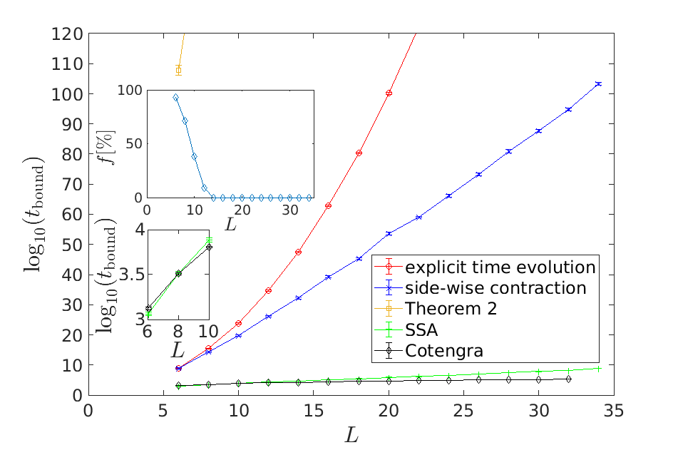
Figure 4: Mean logarithms of the bounds obtained for the classical computation time based on explicit time evolution ($TL^{2}2^{2+L^{2}-\#(\mathrm{idle\ qubits})}$), side-wise contraction ($2^{1+4FL}L$), the second bound of Theorem 2, the bound from the SSA, and the number of scalar operations required by Cotengra [32], averaged over 100 quantum circuit realizations of IQP quantum circuits. Top inset: Percentage of realizations for which the SSA (without any additional optimizations) outperforms Cotengra. Bottom inset: Zoom-in of the main figure for small system sizes. Error bars denote the standard error of the mean of the logarithms.

1. IQP quantum circuits: Here, we apply the procedure to IQP quantum circuits [35] with single- and two-qubit gates: In each of the $T$ time steps, a single-qubit gate is acted on a qubit with probability $7/8$ [corresponding to a randomly chosen phase gate $\mathrm{diag}(1,e^{i\pi m/4}),\ m\in\{0,1,\ldots,7\}$], and afterwards two-qubit gates act on all nearest-neighbor pairs of qubits which have not yet been acted on in this time step with probability $p=3/4\cdot\gamma\ln(N)/N$. The prefactor of $3/4$ corresponds to randomly chosen gates $\mathrm{diag}(1,1,1,i^{m}),\ m\in\{0,1,2,3\}$. The results for $T=L^{2}$ and $\gamma=3$ are shown in Fig. 4. While the bound from Theorem 2 is large, the one from the SSA performs many orders of magnitude better, also beating naive contraction schemes and the state-of-the-art method Cotengra [32] for most (some) quantum circuit realizations for $L\leq 8$ ($L\leq 12$).

2. Google Sycamore-type quantum circuits: We consider a quantum circuit of the type of Ref. [17], where each qubit (apart from the edge ones) is acted on by one single-qubit gate and one two-qubit gate coupling it to a nearest neighbor per “cycle”. There are eight cycles of such couplings, which are repeated periodically (i.e., with two two-qubit gates acting on the same nearest neighbor). We assume that there are $q$ such periods of eight cycles and that in each period a given qubit is inaccessible with probability $p$, i.e., no single- or two-qubit gate acts on it for the entire period. We calculated the corresponding bounds for $q=5$ and $p=0.88$ (which is below the percolation threshold [36]) and averaged over 100 quantum circuit realizations for each $L$. The results, presented in detail in the SM, indicate that the bound of Theorem 2 outperforms naive contraction schemes for most quantum circuit realizations for $L\geq 1600$. (We found it to be superior for some quantum circuit realizations already for $L\geq 400$.)

3. (2+1)-dimensional random quantum circuits: We consider a quantum circuit of $T=\alpha L$ time steps. At each time step, nearest-neighbor gates are densely placed with a random orientation unless there is a cavity in the quantum circuit. These cavities have size $S\times S\times S$ in space-time. Their maximum number $v$ is chosen randomly according to a Poisson distribution with parameter $\lambda$ corresponding to a probability $p_{v}(\lambda)$. The up to $v$ cavities are placed randomly in the quantum circuit [coordinates $(x,y,t)$]; each one appears with probability $p(x,y,t)=\exp\left[-\left(x^{2}/L^{2}+y^{2}/L^{2}+t^{2}/T^{2}\right)/\sigma^{2}\right]$. The results for $S=5$, $\alpha=0.1$, $\sigma=10$, and $\lambda=5\cdot 10^{4}(L/200)^{3.5}$ (displayed in the SM) are similar to the ones of the previous example, but with a sharper transition. They indicate that the bound of Theorem 2 improves over the one for side-wise contraction and explicit time evolution for most quantum circuit realizations already for $L\geq 250$.

Conclusion. – We have used the SST to derive analytical upper bounds on the classical contraction runtime of finite-ranged higher-dimensional tensor networks. We proved similar upper bounds on the classical simulation time of arbitrary higher-dimensional quantum circuits with single- and finite-ranged two-qubit gates. While these bounds improve over naive contraction schemes only for relatively large system sizes, we showed that, in practice, far better upper bounds are obtained with the SSA, which also outperform a state-of-the-art method for certain quantum circuits of relevant sizes. Our approach will find important applications in the context of classical benchmarks for quantum simulations and help to determine the regime where they do not meet the criterion of quantum supremacy. We envision particularly powerful classical tensor network contraction schemes as a result of combining our algorithm with other heuristic methods, such as the stem optimization technique of Ref. [20], or the index slicing approach of Ref. [12].

10:  Positions $\mathcal{P}=\{\mathbf{p}_{1},\mathbf{p}_{2},\ldots,\mathbf{p}_{s}\}\in\mathbb{R}^{d}$ of centers of spheres, representing $s$ tensors, and the corresponding radii $\mathcal{R}=\{r_{1},r_{2},\ldots,r_{s}\}$.

21:  Compute $\Pi(\mathcal{P})=\{\Pi(\mathbf{p}_{1}),\Pi(\mathbf{p}_{2}),\ldots,\Pi(\mathbf{p}_{s})\}$, where $\Pi$ denotes the stereographic projection from $\mathbb{R}^{d}$ to the unit sphere $S^{d}\subset\mathbb{R}^{d+1}$.

32:  Compute a centerpoint [37] $\mathbf{c}\in\mathbb{R}^{d+1}$ of $\Pi(\mathcal{P})$, i.e., all hyperplanes containing $\mathbf{c}$ divide the set of points $\{\Pi(\mathbf{p}_{1}),\Pi(\mathbf{p}_{2}),\ldots,\Pi(\mathbf{p}_{s})\}$ in a ratio $(d+1)\,$:$\,1$ or less. $\mathbf{c}$ is calculated efficiently by randomly selecting subsets $\mathcal{S}\subset\Pi(\mathcal{P})$ of size $|\mathcal{S}|=a$ and calculating their centerpoints $\mathbf{c}_{\mathcal{S}}$ using Linear Programming on $\mathcal{O}(a^{d+1})$ linear inequalities of $d+1$ variables. (For any $\delta>0$ this approach produces a $(d+1+\delta)\,$:$\,1$ centerpoint with high probability if $a>g(\delta,d+1)$, where $g$ is an $s$-independent function [38, 39, 40], making the approach scalable.)

43:  Compute an orthogonal matrix $R\in\mathbb{R}^{(d+1)\times(d+1)}$ such that $R\,\mathbf{c}=(0,0,\ldots,0,||\mathbf{c}||)$.

54:  Define the dilatation map $D_{\alpha}=\Pi\circ(\alpha\mathbb{1})\circ\Pi^{-1}$, where $\alpha=\sqrt{(1-||\mathbf{c}||)/(1+||\mathbf{c}||)}$.

65:  Choose a random great circle $C$ on $S^{d}$. The center of $S^{d}$ can be shown to be a centerpoint of $D_{\alpha}\circ R\circ\Pi(\mathcal{P})$ [28], i.e., $C$ divides these points in a ratio $1\,$:$\,(d+1+\delta)$ or better. $C$ gives rise to a sphere $S\subset\mathbb{R}^{d}$ after transforming back to the original $\mathbb{R}^{d}$ space, which (generically) satisfies Eq. (2).

76:  Calculate the sphere $S=\Pi^{-1}\circ R^{\top}\circ D_{\alpha}^{-1}(C)$. It can be proven that $S$ also satisfies Eq. (1) with probability at least $1/2$ [28] for sufficiently small $\delta>0$.

87:  Check, taking account of the radii $\mathcal{R}$, if Eqs. (1) and (2) are satisfied. If not, choose another great circle $C^{\prime}\in S^{d}$ and repeat steps 5 and 6 until successful. (In general, if any of the above approaches is successful with probability $\rho=\mathcal{O}(1)$, it has to be carried out $1/\rho$ times on average.)

7:  Sphere $S$, $\Gamma_{O}(S)$, $\Gamma_{E}(S)$, $\Gamma_{I}(S)$.

Algorithm 1 Sphere Separator Algorithm [28]

Appendix A Numerical implementation

The proof of the Sphere Separator Theorem (SST), used in the main text, is constructive [28], and there also exists an algorithm to efficiently calculate the corresponding sphere separator. Here we show how this algorithm can be used to compute a separator hierarchy satisfying the bounds of Theorems 1 and 2. As illustrated with examples in the main text (see also next section), the separator hierarchies obtained in practice correspond to much lower classical runtimes.

The algorithm to calculate the sphere separators of Theorems 1 and 2 is a probabilistic approach and was first presented in Ref. [28]. In our case, Algorithm 1 (summarized above) has to be applied $\mathcal{O}(n)$ times, where $n$ is the number of tensors. The separator hierarchy (see main text) allows us to provide an upper bound on the classical simulation time of the specific tensor network Algorithm 1 is applied to: At the lowest level of the separator hierarchy are clusters of few tensors. The contraction of each of these clusters contributes $\mathcal{O}(1)$ to the overall contraction time. For a given tensor network and computed separator hierarchy, we use a greedy algorithm to upper bound the contraction time of the small clusters to individual tensors at the bottom of the separator hierarchy. At all higher levels, the separator hierarchy uniquely specifies in which order the corresponding tensors have to be pairwise contracted, such that the corresponding computational times can be calculated explicitly. The obtained upper bound for the overall contraction time is at least as good as the general bound of Theorem 2, but, in general, many orders of magnitude better.

Appendix B Additional numerical data

The practical performance of Algorithm 1 can be gathered from Fig. 4 in the main text for short-range instantaneous quantum polynomial-time (IQP) quantum circuits. In Fig. 5a we show the same data for Sycamore-type quantum circuits [35] acting on an $L\times L$ lattice of qubits. Fig. 5b displays our numerical data for (2+1)-dimensional random quantum circuits (without the results of Algorithm 1), also for square lattices.

Figure 5: a: Mean logarithms of the bounds obtained for the classical computation time based on explicit time evolution ($TL^{2}2^{2+L^{2}-\#(\mathrm{idle\ qubits})}$), side-wise contraction ($2^{1+4FL}L$), Theorem 2, and Algorithm 1 averaged over 100 realizations of Sycamore-type quantum circuits. Error bars denote the standard error of the mean of the logarithms. Inset: Same bounds (except the one of Algorithm 1) for large system sizes. b: Same for 100 realizations of random quantum circuits with Poisson-distributed numbers of cavities (save the Algorithm 1 results). Inset: Fraction $f$ of quantum circuits for which the bound of Theorem 2 improves over side-wise contraction. It improves over explicit time evolution for all realizations for $L\geq 200$ (not shown).

References

- Eisert [2013] J. Eisert, Entanglement and tensor network states,, Model. Simu. 9, 520 (2013).
- Orús [2019] R. Orús, Tensor networks for complex quantum systems, Nat. Rev. Phys. 1, 538 (2019).
- Tagliacozzo et al. [2014] L. Tagliacozzo, A. Celi, and M. Lewenstein, Tensor Networks for Lattice Gauge Theories with Continuous Groups, Phys. Rev. X 4, 041024 (2014).
- Silvi et al. [2014] P. Silvi, E. Rico, T. Calarco, and S. Montangero, Lattice gauge tensor networks, New J. Phys. 16, 103015 (2014).
- Zohar et al. [2015] E. Zohar, M. Burrello, T. B. Wahl, and J. I. Cirac, Fermionic Projected Entangled Pair States and Local Gauge Theories, Ann. Phys. 363, 385 (2015).
- Zohar et al. [2016] E. Zohar, T. B. Wahl, M. Burrello, and J. I. Cirac, Projected Entangled Pair States with non-Abelian gauge symmetries: An study, Ann. Phys. 374, 84 (2016).
- Bañuls et al. [2019] M. C. Bañuls, K. Cichy, J. I. Cirac, K. Jansen, and S. Kühn, Tensor Networks and their use for Lattice Gauge Theories, PoS(LATTICE2018), 334 (2019).
- Markov and Shi [2008] I. L. Markov and Y. Shi, Simulating Quantum Computation by Contracting Tensor Networks, SIAM J. Comp. 38, 963 (2008).
- Ferris and Poulin [2014] A. J. Ferris and D. Poulin, Tensor Networks and Quantum Error Correction, Phys. Rev. Lett. 113, 030501 (2014).
- Guo et al. [2019] C. Guo, Y. Liu, M. Xiong, S. Xue, X. Fu, A. Huang, X. Qiang, P. Xu, J. Liu, S. Zheng, H.-L. Huang, M. Deng, D. Poletti, W.-S. Bao, and J. Wu, General-Purpose Quantum Circuit Simulator with Projected Entangled-Pair States and the Quantum Supremacy Frontier, Phys. Rev. Lett. 123, 190501 (2019).
- Pan et al. [2020] F. Pan, P. Zhou, S. Li, and P. Zhang, Contracting Arbitrary Tensor Networks: General Approximate Algorithm and Applications in Graphical Models and Quantum Circuit Simulations, Phys. Rev. Lett. 125, 060503 (2020).
- Huang et al. [2021] C. Huang, F. Zhang, M. Newman, X. Ni, D. Ding, J. Cai, X. Gao, T. Wang, F. Wu, G. Zhang, H.-S. Ku, Z. Tian, J. Wu, H. Xu, H. Yu, B. Yuan, M. Szegedy, Y. Shi, H.-H. Zhao, C. Deng, and J. Chen, Efficient parallelization of tensor network contraction for simulating quantum computation, Nat. Comp. Sci. 1, 578 (2021).
- Farrelly et al. [2021] T. Farrelly, R. J. Harris, N. A. McMahon, and T. M. Stace, Tensor-Network Codes, Phys. Rev. Lett. 127, 040507 (2021).
- [14] M. Levental, Tensor Networks for Simulating Quantum Circuits on FPGAs, arXiv:2108.06831 .
- Napp et al. [2022] J. C. Napp, R. L. La Placa, A. M. Dalzell, F. G. S. L. Brandão, and A. W. Harrow, Efficient Classical Simulation of Random Shallow 2D Quantum Circuits, Phys. Rev. X 12, 021021 (2022).
- Stoudenmire and Schwab [2016] E. Stoudenmire and D. J. Schwab, Supervised Learning with Tensor Networks, Adv. Neur. Info. Proc. Sys. 29, 4799 (2016).
- Arute et al. [2019] F. Arute, K. Arya, R. Babbush, D. Bacon, J. C. Bardin, et al., Quantum supremacy using a programmable superconducting processor, Nature (London) 574, 505 (2019).
- Guo et al. [2021] C. Guo, Y. Zhao, and H.-L. Huang, Verifying Random Quantum Circuits with Arbitrary Geometry Using Tensor Network States Algorithm, Phys. Rev. Lett. 126, 070502 (2021).
- Gray and Kourtis [2021a] J. Gray and S. Kourtis, Hyper-optimized tensor network contraction, Quantum 5, 410 (2021a).
- [20] C. Huang, F. Zhang, M. Newman, J. Cai, X. Gao, Z. Tian, J. Wu, H. Xu, H. Yu, B. Yuan, M. Szegedy, Y. Shi, and J. Chen, Classical Simulation of Quantum Supremacy Circuits, arXiv:2005.06787 .
- Pan et al. [2022] F. Pan, K. Chen, and P. Zhang, Solving the sampling problem of the Sycamore quantum supremacy circuits, Phys. Rev. Lett. 129, 090502 (2022).
- [22] F. Pan and P. Zhang, Simulating the Sycamore quantum supremacy circuits, arXiv:2103.03074 .
- Liu et al. [2021] Y. Liu, X. Liu, F. Li, H. Fu, Y. Yang, J. Song, P. Zhao, Z. Wang, D. Peng, H. Chen, et al., Closing the “quantum supremacy” gap: achieving real-time simulation of a random quantum circuit using a new sunway supercomputer, in Proceedings of the International Conference for High Performance Computing, Networking, Storage and Analysis (2021) pp. 1–12.
- Dumitrescu et al. [2018] E. F. Dumitrescu, A. L. Fisher, T. D. Goodrich, B. D. Humble, Travis S. Sullivan, and A. L. Wright, Benchmarking treewidth as a practical component of tensor network simulations, Plos One 13, 12 (2018).
- [25] J. M. Dudek, L. Dueñas Osorio, and M. Y. Vardi, Efficient Contraction of Large Tensor Networks for Weighted Model Counting through Graph Decompositions, arXiv:1908.04381 .
- [26] T. Ayral, T. Louvet, Y. Zhou, C. Lambert, E. M. Stoudenmire, and X. Waintal, A density-matrix renormalisation group algorithm for simulating quantum circuits with a finite fidelity, arXiv:2207.05612 .
- Lipton and Tarjan [1979] R. J. Lipton and R. E. Tarjan, A Separator Theorem for Planar Graphs, SIAM Journal on Applied Mathematics 36, 177 (1979).
- Miller et al. [1997] G. L. Miller, S.-H. Teng, W. Thurston, and S. A. Vavasis, Separators for sphere-packings and nearest neighbor graphs, Journal of the ACM (JACM) 44, 1 (1997).
- Kourtis et al. [2019] S. Kourtis, C. Chamon, E. Mucciolo, and A. Ruckenstein, Fast counting with tensor networks, SciPost Physics 7 (2019).
- [30] Y. Liu, The Complexity of Contracting Planar Tensor Network, arXiv:2001.10204 .
- Huang et al. [2020] C. Huang, M. Newman, and M. Szegedy, Explicit lower bounds on strong quantum simulation, IEEE Transactions on Information Theory 66, 5585 (2020).
- Gray and Kourtis [2021b] J. Gray and S. Kourtis, Hyper-optimized tensor network contraction, Quantum 5, 410 (2021b).
- Smith and Wormald [1998] W. Smith and N. Wormald, Geometric separator theorems and applications, in Proceedings 39th Annual Symposium on Foundations of Computer Science (Cat. No.98CB36280) (IEEE Comput. Soc, 1998).
- Djidjev and Venkatesan [1997] H. N. Djidjev and S. M. Venkatesan, Reduced constants for simple cycle graph separation, Acta Informatica 34, 231 (1997).
- Bremner et al. [2017] M. J. Bremner, A. Montanaro, and D. J. Shepherd, Achieving quantum supremacy with sparse and noisy commuting quantum computations, Quantum 1, 8 (2017).
- Kesten [1980] H. Kesten, The critical probability of bond percolation on the square lattice equals 1/2, Commun. Math. Phys. 74, 41 (1980).
- Edelsbrunner [1987] H. Edelsbrunner, Algorithms in Combinatorial Geometry (Springer Berlin Heidelberg, 1987).
- Vapnik and Chervonenkis [1971] V. N. Vapnik and A. Y. Chervonenkis, Theory Prob. Appl. 16, 264 (1971).
- Haussler and Welzl [1987] D. Haussler and E. Welzl, -nets and simplex range queries, Discrete & Computational Geometry 2, 127 (1987).
- Teng [1991] S.-H. Teng, Point, Spheres, and Separators: A unified geometric approach to graph partitioning, Ph.D. thesis, CMU-CS-91-184, School of Computer Science, Carnegie-Mellon Univ., Pittsburgh, Pa. (1991).