A Recursive Partitioning Approach for Dynamic Discrete Choice Modeling in High Dimensional Settings

Abstract

Dynamic discrete choice models are widely employed to answer substantive and policy questions in settings where individuals’ current choices have future implications. However, estimation of these models is often computationally intensive and/or infeasible in high-dimensional settings. Indeed, even specifying the structure for how the utilities/state transitions enter the agent’s decision is challenging in high-dimensional settings when we have no guiding theory. In this paper, we present a semi-parametric formulation of dynamic discrete choice models that incorporates a high-dimensional set of state variables, in addition to the standard variables used in a parametric utility function. The high-dimensional variable can include all the variables that are not the main variables of interest but may potentially affect people’s choices and must be included in the estimation procedure, i.e., control variables. We present a data-driven recursive partitioning algorithm that reduces the dimensionality of the high-dimensional state space by taking the variation in choices and state transition into account. Researchers can then use the method of their choice to estimate the problem using the discretized state space from the first stage. Our approach can reduce the estimation bias and make estimation feasible at the same time. We present Monte Carlo simulations to demonstrate the performance of our method compared to standard estimation methods where we ignore the high-dimensional explanatory variable set.

Keywords: Structural Models, Dynamic Discrete Choice Models, Machine Learning, Recursive Partitioning

1 Introduction

Consumers’ choices are not solely a function of the utility they get in the current stage in many settings. They might forgo a choice with higher current utility for a better stream of utilities in the future. Buying a new car instead of keeping an old car, getting higher education, and investing in retirement plans are examples of such choices. Estimating the underlying primitives of an agent’s behavior in these settings requires incorporating the current utility she gets and her future stream of utilities from a choice.

In the conventional dynamic discrete choice modeling approaches, researchers calculate the value of being in each state of the problem space. This value, a.k.a value function, is equal to the discounted sum of all the future utilities an agent gets from making optimal choices in the future starting from that given state. Researchers calculate the value functions by solving a dynamic programming problem using the Bellman equation (Smammut and Webb, 2010). Two limitations make the estimation of these models challenging. First, solving the dynamic programming problem is computationally expensive and infeasible in high-dimensional data settings. Second, researchers must make some assumptions on the data generating process in the unobserved part of the state space to make the estimation possible. For example, one common assumption is that the observable part of the state in time $t$ is independent of the unobservable part of the state in the previous time period. As a result, it becomes essential to incorporate all the potential variables that affect agents’ decisions and state transitions to avoid violation of these assumptions, even if these variables are not the main focus of the research problem at hand.

These two limitations force an accuracy-computation trade-off to researchers. On the one hand, limiting the number of variables in the estimation procedure, in the favor computational feasibility, increases the chance of violating the required estimation assumption. On the other hand, adding more explanatory variables makes the computation infeasible as adding each variable increases the size of the state space exponentially (Rust, 1997). In addition to the accuracy concerns, model specification choices such as selecting the appropriate covariates and discretizing the state space are challenging, especially in complex and high-dimensional settings. Researchers usually have little intuition about which covariates to select or how to discretize the state space (Semenova, 2018). As a result, many estimation approaches avoid this trade-off by proposing value function estimation procedures that do not require solving a dynamic programming problem (Hotz and Miller, 1993; Hotz et al., 1994; Keane and Wolpin, 1994; Norets, 2012; Arcidiacono et al., 2013; Semenova, 2018).

Besides the concerns for estimation assumptions, the data-gathering trends in the industry calls for more high-dimensional friendly approaches in dynamic choice modeling. Gathering data has become a necessary part of businesses of all sizes. Companies create massive databases of users’ behavioral and contextual data, hoping to turn the data into knowledge and enhance the quality of their services, and marketing interventions. Demographic and behavioral data is used for designing personalized services, promotions, and prices. The advent of high-dimension friendly approaches has made it possible for companies to exploit all the available information to extract knowledge from consumers. The hyper-parameter optimization procedure implemented within these algorithms ensures that the model is generalizable to the data-generating process, not the training dataset. Overfitting is of foremost importance in high-dimensional settings as it is easier for the algorithm to model noise instead of signal (Zimek et al., 2012). These methods, nevertheless, are not appropriate for modeling dynamic choice modeling settings, as they do not incorporate the future implications of a decision into account. Estimation of dynamic choice models in high-dimensional settings has remained a rewarding research topic open to investigation.

This paper proposes a novel approach that let researchers control for a high-dimensional variable set $\operatorname{\mathbf{Q}}$, in addition to the conventional independent variable set $\operatorname{\mathbf{X}}$ in dynamic discrete choice modeling. We reduce the dimensionality of $\operatorname{\mathbf{Q}}$ using a data-driven discretization approach based on recursive partitioning. In our framework, we distinguish between the state space discretization and estimation, and separate these two steps in our framework. We define the term perfect discretization as a discretization where all the points in the same partition have a similar decision and transition probabilities. We reformulate the DDC problem using the perfect discretization definition. We then propose an algorithm for discretization and prove that the discretization offered by our algorithm converges to a perfect discretization. Researchers can then use any conventional algorithm for the estimation of parameters in for the estimation stage using the discretized state space offered in the first stage.

Our dimension reduction method has several desirable properties that makes it convenient to use and applicable in many settings. First, we separate the estimation and discretization tasks and define a general discretization criterion that does not depend on parametric assumptions of the estimation step. This property makes the algorithm robust to the parametric assumption of the estimation step. Furthermore, the discretization algorithm does not impose any limitation on the estimation method one can use in the second stage. The discretization algorithm converts the high-dimensional variable set $\operatorname{\mathbf{Q}}$ to a categorical variable $\operatorname{\mathcal{P}}$. Researchers can then use the new independent variable set $\{\operatorname{\mathbf{X}},\operatorname{\mathcal{P}}\}$ with any conventional DDC estimation method that can handle categorical variables. In addition, the algorithm can be used for discretization in both finite and infinite time horizon settings.

Second, our discretization algorithm inherits the desirable properties of recursive partitioning-based algorithms. The time complexity of our method is linear with respect to the dimensionality of $\operatorname{\mathbf{Q}}$. If the number of dimensions in $\operatorname{\mathbf{Q}}$ doubles, the discretization time of our algorithm doubles at most. It is a substantial computational saving compared to conventional methods such as nested fixed-point, whose time complexity is exponential with respect to the dimensionality of the independent variable set. In addition, our algorithm is robust to scale and irrelevant variables. Our discretization algorithm offers the same discretization for $\operatorname{\mathbf{Q}}$ and any transformation of $\operatorname{\mathbf{Q}}$ that does not change the ordinality of observations. Furthermore, the algorithm can be implemented in a parallelized way, making its execution pretty fast over distributed systems and servers with many cores. These desirable properties make it possible for researchers and industry users to benefit from all their available information in the discretization procedures without domain expertise or computational concerns.

Third, in addition to the agents’ choice data, our algorithm uses the rich information available in the state transition data to reduce the state space dimension. It is a novel approach given that researchers usually regard the state space transition as a nuisance parameter; they non-parametrically estimate it in the first step of DDC modeling. The algorithm’s capability to use the variation in agents’ decision and state transition for dimension reduction makes it a more efficient algorithm than when only the decision part is used for discretization. Additionally, our algorithm learns the relative importance of these two parts of agents’ behavior during hyperparameter optimization and assigns an optimal weight to each part of the data. As we show in our simulation study section, optimizing the relative importance of these two can lead to considerable gains in optimal discretization.

Our paper is organized as the following. In section 2, we review the current literature on the estimation of dynamic discrete choice models and proposed methods for their estimation in high-dimension. We also touch upon the recursive partitioning algorithm and its extensions designed for estimation in different modeling settings. In section 3, we formulate the problem at hand by explaining the components of dynamic discrete choice models, pointing to the curse of dimensionality, defining perfect discretization, and reformulating the estimation of DDC problems in the discretized space. In section 4 we describe our discretization approach, discuss hyper-parameter optimization and model selection, and highlight the properties of the algorithm. We run two simulation studies to take a deeper look into this problem in section 5. In the first simulation study, we highlight the importance of controlling for estimation assumptions. In the second simulation study, we highlight the value of state transition data and our algorithm’s ability to exploit the rich information in state transition for discretization. Section 7 concludes.

2 Related Literature

First, our paper is related to the literature of estimating dynamic discrete choice modeling in high-dimensional settings and breaking the curse of dimensionality in DDC modeling. The Bellman’s equation in DDC modeling rarely has an analytical solution, and the dynamic programming problem of calculating the value function is usually solved numerically (Rust, 1997). Unfortunately, the computational complexity of this numerical estimation increases exponentially as the number of explanatory variables increase. Many solutions have been proposed to break this course of dimensionality, and make estimation of DDC models in high-dimensional settings feasible.

Hotz and Miller (1993) shows that the value function can sometimes be estimated from the probability that a specific choice occurs in any given state space. This so-called Conditional Choice Probability (CCP) method makes the DDC estimation problem possible in high dimensions. However, CCP techniques have two limitations: i) using CCP methods is not always possible since they rely on some particular structures in the state space, ii) to conduct counterfactual analysis, researchers usually need to solve the full model once using NFXP. Several methods used simulation to estimate the approximation of full solution methods (Keane and Wolpin, 1994; Hotz et al., 1994). One can use the non-parametric estimations of choice probabilities and state transitions to draw a choice and a realized state given a choice and use simulations to solve the DDC problem.

Another stream of research tries to resolve the dimensionality problem by approximating the value function. Methods such as parametric policy iteration (Benitez-Silva et al., 2000), and sieve value function iteration (Arcidiacono et al., 2012) estimate the value function by assuming a flexible functional form for it. Nonetheless, these methods work well when there are a set of basis functions that provide a good approximation of the value function (Rust, 2000). A more recent body of literature has tried to use the advances in machine learning and methods such as neural networks to solve DDC problems. Norets (2012) uses an artificial neural network to estimate the value function taking state variables and parameters of interest as input. Semenova (2018) offers a simulation-based method using machine learning. She estimates the state transition and decision probabilities by machine learning models in the first stage and uses them to find the underlying decision parameters in the second stage.

Su and Judd (2012) proposes yet another approach to solve the curse of dimensionality problem in dynamic discrete choice modeling called MPEC. They formulate the dynamic discrete choice problem as a constrained maximization problem where likelihood function is the maximization objective, and the bellman equations are the constraints. Dubé et al. (2012) show that MPEC is applicable to a broader set of problems. MPEC method reduces the computational complexity as it does not need to solve the bellman equation and calculate the value function at each guess of the structural parameters. Nevertheless, MPEC algorithm is still not applicable in high-dimensional settings without proper discretization of the state space. Although we do not solve the structural equation at each iteration of MPEC algorithm, we estimate the value function for each point of the state space. As the number of variables increases, the size of the state space increases exponentially, and as a result, using MPEC becomes computationally infeasible.

Our algorithm adds to this literature by offering a method to break the curse of dimensionality through discretization rather than value function approximation. We argue that state-space discretization and parameter estimation are two separate tasks. In fact, our discretization algorithm can be used together with any of the above algorithms: researcher uses our algorithm to reduce the dimensionality of a high-dimensional state space $\operatorname{\mathbf{Q}}$ to a one-dimensional categorical variable $\operatorname{\mathcal{P}}$ in the first stage, and then use $\operatorname{\mathcal{P}}$ in addition to other independent variables $\operatorname{\mathbf{X}}$ for estimation of parameters using any of the above algorithms in the second stage. This procedure lets the researcher control for a high-dimensional covariate $\operatorname{\mathbf{Q}}$ at a low computational cost.

Second, our paper contributes to the literature of estimation using recursive partitioning. Breiman et al. (1984) work gave birth to the Classification and Regression Trees (CART) algorithm, one of the earliest and well-known algorithms for estimation using recursive partitioning. Ensemble methods combine several trees to produce better performance than a single tree. The Random Forest algorithm (Breiman, 2001) is based on the idea of generating thousand of such trees, each on a subsample of data and covariates, and average the estimates of trees for prediction. While recursive partitioning has been used for prediction tasks, there has been a recent development for using recursive partitioning for different purposes. Athey and Imbens (2016) has used the recursive partitioning approach for the heterogeneous causal effect estimation task. They offer a method to partition the data into subgroups that differ in the magnitude of their treatment effects. Athey et al. (2019) propose the Generalized Random Forests (GRF) algorithm, a method for non-parametric statistical estimation that can be used to fit any quantity of interest. They use their approach to develop new estimation methods for different statistical tasks, including non-parametric quantile regression, conditional average partial effect estimation, and heterogeneous treatment effect estimation via instrumental variables. However, their method is limited to the static estimation settings as their algorithm does not incorporate the state transitions in discretization. Our algorithm adds to this literature by proposing a novel use of recursive partitioning to estimate dynamic models. We develop a new approach for formulating the objective function that enables us to use the state transition data during recursive partitioning.

Third, our paper indirectly contributes to the literature of unobserved heterogeneity in dynamic discrete choice modeling. A potential solution for concerns regarding DDC modeling assumptions on the unobservable part of state space is to use latent class models. Arcidiacono and Jones (2003) and Arcidiacono and Miller (2011) have suggested EM-based algorithms to account for unobservable parts of the state space and their transitions. Nevertheless, these algorithms suffer from several limitations that make them impractical in circumstances where we have quite a few unobservable states. Besides, these algorithms are not guaranteed to converge to the global maximum (Wu, 1983). Even though our algorithm does not directly capture the effect of unobservables, its ability to capture the effects of a high-dimensional variable set alleviates the concerns from the unobservable part of the state space. Similar to the latent class models in DDC estimation, our algorithms assign a category to each observation. However, in contrast to the EM-based algorithms, which use a latent class to capture the explained variation in the dependent variable, our algorithm uses a high-dimensional variable set to potentially explain the variation.

3 Problem Definition

We consider the discrete choice problem from the perspective of a forward-looking single agent, denoted by $i\in\{1\dots N\}$. In every period $t$, the agent chooses between $j=1\ldots J$. options. $i$’s decision in period $t$ is denoted by $d_{it}$, and $d_{it}=j$ indicates that agent $i$ has chosen option $j$ in period $t$. The agent’s decision is not only the function of her utility in current state ($s_{it}$), but also her expectation of her utility in all her future states given decision $d_{it}$. We assume that the agent’s state is composed of three sets of variables.

1. A set of observable low-dimensional state variables $x_{it}\in\operatorname{\mathbf{X}}$.

2. A set of observable high-dimensional state variables $q_{it}\in\operatorname{\mathbf{Q}}$.

3. Unobservable state variable $\epsilon_{it}$, which is a $J\times 1$ vector each associated with one of the alternatives observed by the agent, but not by the researcher.

$\operatorname{\mathbf{X}}$ represents state variables for which we have some a priori theory, i.e., we know how the parametric form in which they enter the utility function. The structural parameters associated with these variables form the main estimands of interest. $\operatorname{\mathbf{Q}}$ denotes state variables that act as nuisance variables in our estimation exercise – they are not the main variables of interest, and we do not have a theory for if and how they influence users’ decisions and state transitions. However, ignoring them can potentially bias the estimates of interest.

In each period $t$, agent $i$ derives an instantaneous flow utility $u(s_{it},d_{it})$, which is a function of her decision $d_{it}$ and her state variables $s_{it}=\{x_{it},q_{it},\epsilon_{it}\}$. The per period utility is additively separable as follows:

$$u(s_{it},d_{it}=j)=\bar{u}(x_{it},q_{it},d_{it}=j;\theta_{1})+\epsilon_{itj},$$ (1)

where $\epsilon_{itj}$ is the error term associated with $j^{th}$ option at time $t$, $\bar{u}(x_{it},q_{it},d_{it}=j;\theta_{1})$ is the deterministic part of the utility from making decision $j$ in state $x_{it},q_{it}$, and $\theta_{1}$ is the set of structural parameters associated with the deterministic part of utility. The state $s_{it}$ transitions into new, but not necessary different, values in each period following decision $d_{it}$. We make three standard assumptions on the state transition process – first order markovian, conditional independence, and IID error terms. These assumptions imply that: (i) $\{s_{it},d_{it}\}$ are sufficient statistics for $s_{it+1}$, (ii) error terms are independent over time, and (iii) errors in the current period affect states tomorrow only through today’s decisions. Thus, we have:

$$\Pr(x_{it+1},q_{it+1},\epsilon_{it+1}|x_{it},q_{it},\epsilon_{it},d_{it})=\Pr(\epsilon_{it+1})\Pr(x_{it+1},q_{it+1}|x_{it},q_{it},d_{it})$$ (2)

We denote the state transition function $\Pr(x_{it+1},q_{it+1}|x_{it},q_{it},d_{it})$ as $g(x_{it+1},q_{it+1}|x_{it},q_{it},d_{it};\theta_{2})$, where $\theta_{2}$ captures the parameters associated with state transition.

Each period, the agent takes into account the current period payoff as well as how her decision today will affect the future, with the per-period discount factor given by $\beta$. She then chooses $d_{it}$ to sequentially maximize the expected discounted sum of payoffs $\operatorname{\mathbb{E}}\left[\sum_{\tau=t}^{\infty}\beta^{\tau}u(s_{i\tau},d_{i\tau})\right]$. Our goal is to estimate the set of structural parameters $\theta=\{\theta_{1},\theta_{2}\}$ that rationalizes the observed decisions and the states in the data, which are denoted by $\{(x_{i1},q_{i1},d_{i1}),\dots,(x_{it},q_{it},d_{it}),\dots,(x_{iT},q_{iT},d_{iT})\}$ for agents $i\in\{1,\ldots,N\}$ for $T$ time periods.

3.1 Challenges

The standard solution is to use a maximum likelihood method and estimates the set of parameters that maximizes the likelihood of observing the data. Given the first-order Markovian and conditional independence assumptions, we can write the likelihood function and estimate the structural parameters as follow

$$\operatorname{\mathcal{L}}(\theta)=\sum_{i=1}^{N}\Bigg{(}\sum_{t=1}^{T}\log\hat{p}(d_{it}|x_{it},q_{it}; \theta_{1})+\sum_{t=2}^{T}\log\hat{g}(x_{it},q_{it}|x_{it-1},q_{it-1},d_{it-1};\theta_{2})\Bigg{)}$$ (3)

$$\theta^{*} =\arg\!\max_{\theta}\operatorname{\mathcal{L}}(\theta)$$

where $\hat{p}(.)$ is the predicted choice probabilities.

However, there are three main challenges in estimating a model in this setting:

• Theory: First, the researcher may lack theory on how the high-dimensional variables $q$ enter the agents’ utility function. For instance, if we consider the example of high-dimensional usage variables in a subscription model, we do not have much theoretical guidance on which of these variables affect users’ utility and how. As such, we cannot make parametric assumptions on the effect of $\operatorname{\mathbf{Q}}$ on decisions and transitions or hand-pick a subset of these variables to include in our model.

• Data: Second, in a high-dimensional setting, we may not have sufficient data in all areas of the state space to model the flow utility and the transitions to/from that area.

• Estimation: Finally, estimation of a discrete choice dynamic model in an extremely high dimensional setting is often computationally infeasible and/or costly. Rust (1987)’s nested-fixed point algorithm requires us to calculate the value function at each combination of the state variables at each iteration of the estimation, which is infeasible in a large state space setting. While two-step methods can overcome estimation challenges in large state-spaces by avoiding the value function iteration, they nevertheless need non-parametric estimates of Conditional Choice Probablities (CCPs) at all values at each state (Hotz and Miller, 1993). This is not possible in a very high dimensional setting with finite data.

Thus, in a finite data, high-dimensional setting where we lack guiding theory, it is not feasible to specify a utility function over $q$ and/or estimate a dynamic discrete choice model using conventional methods. Therefore, we need a data-driven approach that reduces dimensionality of $\operatorname{\mathbf{Q}}$ in an intelligent fashion.

3.2 Dimensionality Reduction using Discretization

Our solution is to recast the problem by mapping $\operatorname{\mathbf{Q}}$ to a lower-dimensional space through data-driven discretization such that $\operatorname{\mathbf{\Pi}}:\operatorname{\mathbf{Q}}\to\operatorname{\mathcal{P}}$, where $\operatorname{\mathcal{P}}=\{1,\dots,k\}$. The goal is similar in spirit to that of Classification and Regression Trees (CART) algorithm used for outcome prediction (Breiman et al., 1984) and the Causal Tree algorithm for estimation of conditional average treatment effects (Athey and Imbens, 2016). These algorithms discretize the covariate space to minimize the heterogeneity of the statistic of interest within a partition. For example, the CART algorithm discretizes the covariate space into disjoint partitions such that observations in the same partition have similar outcome values/class. Similarly, the Causal Tree algorithm discretizes the state space such that observations within the same partition have similar treatment effects. However, the high-level intuition from the static estimation of CART/causal tree cannot be directly translated to dynamic discrete choice models. Therefore, our first step is to outline the characteristics of a suitable discretization. In $\S$3.2.1 we formally define the term perfect discretization as a discretization wherein observations with similar behavior are pooled together in the same partition. Then in, $\S$3.2.2, we present the reformulated problem in the lower-dimensional space.

3.2.1 Properties of a Good Discretization

We now discuss some basic ideas that a good discretization should capture. First, some variables in $\operatorname{\mathbf{Q}}$ may be irrelevant to our estimation procedure, i.e., they have no effect on utilities or state transitions. A good data-driven discretization should be able to neglect these variables and thus be robust to irrelevant variables. Second, our discretization approach has to be entirely non-parametric since we not have any theory on how variables in $\operatorname{\mathbf{Q}}$ affect agents’ utilities and state transitions. Finally, the discretization should be generalizable, i.e., it should be valid outside the training data. Formally, we define the term perfect discretization as follows:

Definition 1.

A discretization $\operatorname{\mathbf{\Pi}}^{*}:\operatorname{\mathbf{Q}}\to\operatorname{\mathcal{P}}$ is perfect if all the points in the same partition have the same decision and incoming and outgoing transition probabilities. That is, for any two points $q,q^{\prime}$ in a partition $\pi\in\operatorname{\mathcal{P}}$, we have:

$$\forall x,x^{\prime}\in\operatorname{\mathbf{X}},q^{\prime\prime}\in\operatorname{\mathbf{Q}},j\in\operatorname{\mathbf{J}}: \Pr(j|x,q)=\Pr(j|x,q^{\prime})$$ (4)

$$\forall x,x^{\prime}\in\operatorname{\mathbf{X}},q^{\prime\prime}\in\operatorname{\mathbf{Q}},j\in\operatorname{\mathbf{J}}: \Pr(x^{\prime},q^{\prime\prime}|x,q,j)=\Pr(x^{\prime},q^{\prime\prime}|x,q^{\prime},j)$$ (5)

$$\forall x,x^{\prime}\in\operatorname{\mathbf{X}},q^{\prime\prime}\in\operatorname{\mathbf{Q}},j\in\operatorname{\mathbf{J}}: \Pr(x,q|x^{\prime},q^{\prime\prime},j)=\Pr(x,q^{\prime}|x^{\prime},q^{\prime\prime},j)$$ (6)

The first equality ensures that the decision probabilities are similar for data points within a given partition $\pi\in\operatorname{\mathcal{P}}$. The second equality asserts the equality of transition probabilities from any two points $q,q^{\prime}$ within the same partition $\pi\in\operatorname{\mathcal{P}}$. Finally, the last equality implies that the transition probabilities to any two points within a partition $\pi$ are equal. Together, these three equalities imply that all the observations within a same $\pi\in\operatorname{\mathcal{P}}$ are similar from both modeling and estimation perspective. Therefore, we do not need to model the heterogeneity within the partition $\pi$. Instead, modeling agents’ behavior at the level of $\operatorname{\mathcal{P}}$ is sufficient.

3.2.2 Formulation of DDC in a discretized space

We now use the definition of perfect discretization and translate the DDC estimation in the $\operatorname{\mathbf{Q}}$-space to the $\operatorname{\mathcal{P}}$-space. Because observations within each partition in a perfect discretization behave similarly, we can project the problem from the $\operatorname{\mathbf{Q}}$-space to the $\operatorname{\mathcal{P}}$-space. That is, $\operatorname{\mathbf{\Pi}}^{*}$ is a sufficient statistic for estimation of state transition and decision probabilities. We can therefore write the probabilities of choices and state transitions in the $\operatorname{\mathcal{P}}$-space as follows:

$$\forall x,x^{\prime}\in\operatorname{\mathbf{X}},q^{\prime\prime}\in\operatorname{\mathbf{Q}},j\in\operatorname{\mathbf{J}}: \Pr(j|x,q)=\Pr(j|x,\operatorname{\mathbf{\Pi}}^{*}(q))$$ (7)

$$\forall x,x^{\prime}\in\operatorname{\mathbf{X}},q^{\prime\prime}\in\operatorname{\mathbf{Q}},j\in\operatorname{\mathbf{J}}: \Pr(x^{\prime},q^{\prime\prime}|x,q,j)=\Pr(x^{\prime},q^{\prime\prime}|x,\operatorname{\mathbf{\Pi}}^{*}(q),j)$$ (8)

$$\forall x,x^{\prime}\in\operatorname{\mathbf{X}},q^{\prime\prime}\in\operatorname{\mathbf{Q}},j\in\operatorname{\mathbf{J}}: \Pr(x,q|x^{\prime},q^{\prime\prime},j)=\frac{\Pr(x,\operatorname{\mathbf{\Pi}}^{*}(q)|x^{\prime},q^{\prime\prime},j)}{N(x,\operatorname{\mathbf{\Pi}}^{*}(q))}$$ (9)

where $N(x,\operatorname{\mathbf{\Pi}}^{*}(q))$ is the number of observations in state $\{x,\operatorname{\mathbf{\Pi}}^{*}(q)\}$.

These three equalities are the counterparts of the relationships shown in Equation (6) in the $\operatorname{\mathcal{P}}$-space. According to the first equality in Equation (9), if the choice probabilities for the observations within a partition $\pi\in\operatorname{\mathcal{P}}$ are the same, then $\{\operatorname{\mathbf{X}},\operatorname{\mathcal{P}}\}$ is a sufficient statistic to capture the choice probabilities. The same argument is true for out-going state transitions. If the probabilities of transition to other states from all points in a partition are similar, we can use the partition instead of points to specify transition (as shown in the second relationship in Equation (9)). Finally, when the probability of transition into all the points within a partition are similar, the probability of moving to a specific point is equal to the probability of transitioning into the partition divided by the number of observations within that partition. That is:

$$\Pr(x,\operatorname{\mathbf{\Pi}}^{*}(q)|x^{\prime},q^{\prime},j) =\sum_{q^{\prime\prime}\in\operatorname{\mathbf{\Pi}}^{*}(q)}\Pr(x,q^{\prime\prime}|x^{\prime},q^{\prime},j)$$

$$=N(x,\operatorname{\mathbf{\Pi}}^{*}(q))\Pr(x,q|x^{\prime},q^{\prime},j),$$

which gives us the third relationship in Equation (9).

We now use the relationships in Equation (9) to reformulate the log likelihood in Equation (3). Given a perfect partitioning $\operatorname{\mathbf{\Pi}}^{*}$, the log likelihood can be written as:

$$\operatorname{\mathcal{L}}(\theta,\operatorname{\mathbf{\Pi}}^{*}) =\sum_{i=1}^{N}\sum_{t=1}^{T}\log p(d_{it}|x_{it},\operatorname{\mathbf{\Pi}}^{*}(q_{it});\theta_{1},\operatorname{\mathbf{\Pi}}^{*})$$

$$+\sum_{i=1}^{N}\sum_{t=2}^{T}\log\frac{g(x_{it},\operatorname{\mathbf{\Pi}}^{*}(q_{it})|x_{it-1},\operatorname{\mathbf{\Pi}}^{*}(q_{it-1}),d_{it-1};\theta_{2},\operatorname{\mathbf{\Pi}}^{*})}{N(x_{it},\operatorname{\mathbf{\Pi}}^{*}(q_{it});\operatorname{\mathbf{\Pi}}^{*})}$$ (10)

Note that the second term in the log-likelihood is obtained by combining the second and third terms in Equation (9) as: $\Pr(x^{\prime},q^{\prime\prime}|x,q,j)=\Pr(x^{\prime},q^{\prime\prime}|x,\operatorname{\mathbf{\Pi}}^{*}(q),j)=\frac{\Pr(x^{\prime},\operatorname{\mathbf{\Pi}}^{*}(q^{\prime\prime})|x^{\prime},\operatorname{\mathbf{\Pi}}^{*}(q),j)}{N(x,\operatorname{\mathbf{\Pi}}^{*}(q^{\prime\prime}))}$.

Finally, since agents within a given partition in $\operatorname{\mathbf{\Pi}}^{*}$ have similar state and choice probabilities, we can conclude that their utility function are also similar. We can formulate the utility function in the $\operatorname{\mathbf{\Pi}}^{*}(q)$-space as follows:

$$u(s_{it},d_{it})=\bar{u}(x_{it},\operatorname{\mathbf{\Pi}}^{*}(q_{it}),d_{it};\theta_{1},\operatorname{\mathbf{\Pi}}^{*})+\epsilon_{itj}$$ (11)

Similarly, we can also write the value function and the choice-specific value function in terms of the discretized state space. Conceptually, once we have a perfect discretization $\operatorname{\mathbf{\Pi}}^{*}$, we can treat $\operatorname{\mathbf{\Pi}}^{*}(q)$ as a categorical variable in addition to $\operatorname{\mathbf{X}}$, and ignore $q$. As such, all the methods available for the estimation of dynamic discrete choice models (e.g., nested fixed point, two-step estimators) are directly applicable here, with $\{\operatorname{\mathbf{X}},\operatorname{\mathcal{P}}\}$ as the state-space. Thus, all the consistency and efficiency properties of the estimator used would directly translate to this setting.

4 Our Discretization Approach

We now present our discretization algorithm. We first explain the recursive partitioning method for a general objective function in $\S$4.1. Next, in $\S$4.2, we formulate a recursive partitioning scheme for the dynamic discrete choice model discussed above. We summarize the properties of our algorithm in $\S$4.2.2. Finally, we discuss model selection and hyper-parameter optimization in $\S$4.3.

4.1 Discretization using Recursive Partitioning

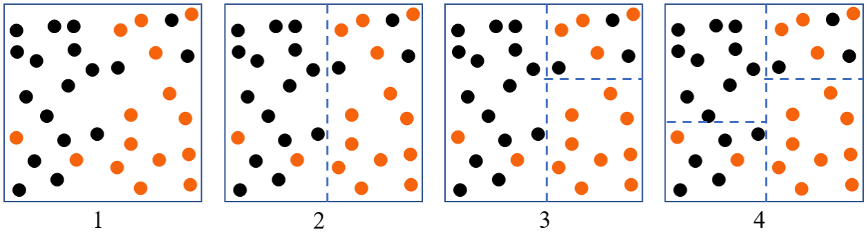
Figure 1: An example of recursive partitioning for a classification task with two explanatory variables and two outcome classes (denoted by orange and black dots).

Recursive partitioning is a meta-algorithm for partitioning a covariate space into disjoint partitions to maximize some objective function. In each iteration, the algorithm uses an objective function as the criterion for selecting the next split among all the potential candidate splits. A split, divides a partition into two along based one of the variables in the covariate space. The following pseudo-code presents a general recursive partitioning algorithm, where the goal is to maximize the objective function $\operatorname{\mathcal{F}}(\operatorname{\mathbf{\Pi}})$.

• Inputs: Objective function $\operatorname{\mathcal{F}}(\operatorname{\mathbf{\Pi}})$ that takes a partitioning $\operatorname{\mathbf{\Pi}}$ as input and outputs a score.

• Initialize $\operatorname{\mathbf{\Pi}}_{0}$ as one partition equal to the full covariate space.

• Do the following until the stopping criterion is met, or $\operatorname{\mathcal{F}}(\operatorname{\mathbf{\Pi}}_{r})=\operatorname{\mathcal{F}}(\operatorname{\mathbf{\Pi}}_{r-1})$

  • For every $\pi\in\operatorname{\mathbf{\Pi}}_{r}$, every $q\in\operatorname{\mathbf{Q}}$, and every value $v\in$ range($q$) in $\pi$

    • $\Delta(\pi,q,v)=\operatorname{\mathcal{F}}(\operatorname{\mathbf{\Pi}}_{r}+\{\pi,q,v\})-\operatorname{\mathcal{F}}(\operatorname{\mathbf{\Pi}}_{r})$

  • $\{\pi^{\prime},q^{*},v^{*}\}=\arg\!\max_{\{\pi,q,v\}}\Delta(\pi,q,v)$

  • $\operatorname{\mathbf{\Pi}}_{r+1}=\operatorname{\mathbf{\Pi}}_{r}+\{\pi^{\prime},q^{*},v^{*}\}$

Figure 1 shows three iterations of recursive partitioning applied to a classification task. The partitioning $\operatorname{\mathbf{\Pi}}$ maps the two-dimensional covariate space into four different partitions.

4.2 Recursive Partitioning for Dynamic Discrete Choice Models

The ultimate goal of our discretization exercise is to estimate $\theta$ by maximizing the likelihood function in Equation (10). To do so, we first need to find a perfect discretization, i.e., a discretization that satisfies Equation (6). Thus, an intermediate goal is to find the partitioning $\operatorname{\mathbf{\Pi}}^{*}$. The key question then becomes what should be the objective function for the recursive partitioning algorithm that helps us achieve the two goals discussed above. One naive approach would be to simply use the log-likelihood shown in Equation (10). However, this is problematic because of three reasons. First, this likelihood is a function of both $\operatorname{\mathbf{\Pi}}^{*}$ and $\theta$. A naive implementation of a recursive partitioning algorithm requires estimating the optimal $\theta$ in every iteration for a given $\operatorname{\mathbf{\Pi}}_{r}$. However, estimating $\theta$ is computationally expensive in a DDC setting because we need to calculate the discounted future utility associated with a given choice to estimate the primitives of agents’ utility function fully. Doing this at every potential split in each iteration of the algorithm is very computationally expensive (and infeasible when the $\operatorname{\mathbf{Q}}$-space is large). Second, the likelihood function contains two sets of outcomes: (i) choice probabilities and (ii) state transition probabilities. Therefore, any data-driven approach to discretize the state space must account for both of these outcomes. This makes the splitting process more complex than usual recursive partitioning algorithms such as CART/causal tree, where there is only one set of estimands to be considered. Third, unlike a standard recursive partitioning algorithm, where we split on all the state variables, here we only split on $\operatorname{\mathbf{Q}}$ since $\operatorname{\mathbf{X}}$s are known (or assumed) to influence outcomes by definition. As such, we need an algorithm which only splits on a subset of state variables ($\operatorname{\mathbf{Q}}$), but considers all the state variables ($\{\operatorname{\mathbf{X}},\operatorname{\mathbf{Q}}\}$) to estimate the choice probabilities and state transitions; see Figure 2 for an example.

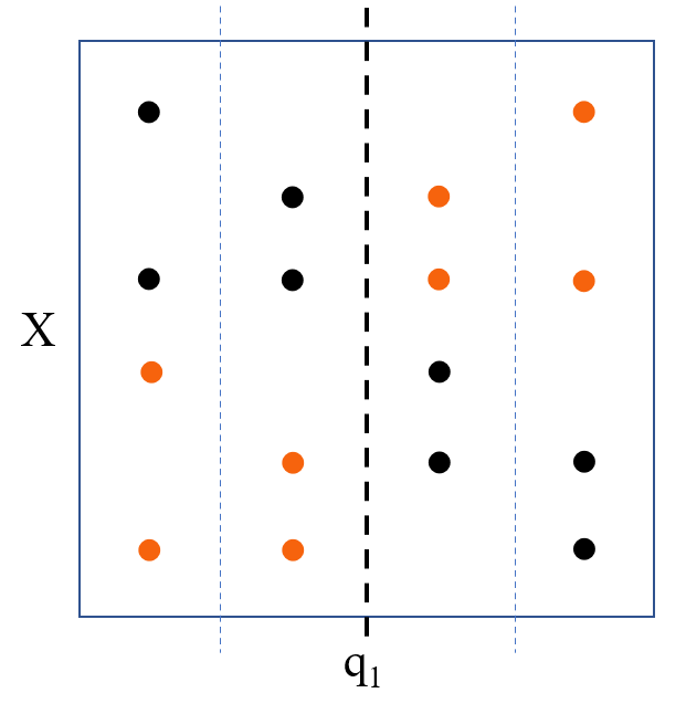
Figure 2: The dashed lines are candidate splits. Orange and black dots are observations with decision 1 and 2 respectively. Agents’ choices across different Xs in the left side of the thick dashed line are different from their choices in the right side.

We design a recursive partitioning method that addresses all these three problems. To address the first problem, we separate the discretization problem from estimation and suggest an objective function for recursive partitioning algorithm that is fully non-parametric, i.e., is not dependent on $\theta$ – thus, its calculation is computationally cheap. Next, to address the second problem, we split our objective function into two sub-objectives, whose relative importance can be learnt from the data using model selection. Finally, to address the third problem, we customize the splitting procedure such that it only splits on $\operatorname{\mathbf{Q}}$ and not $\operatorname{\mathbf{X}}$. We discuss these ideas in detail below.

4.2.1 Nonparametric Objective Function

As we discussed in $\S$3.2.2, we can estimate the primitives of agents’ utilities and state transitions by maximizing the log-likelihood shown in Equation (10). This likelihood is a function of both the primitive parameters and the discretization $\operatorname{\mathbf{\Pi}}^{*}$. Nevertheless, we do not need to solve the maximization problem on both dimensions simultaneously. Conceptually, the discretization goal is to separate $\operatorname{\mathbf{Q}}$ into buckets such that observations within the same bucket behave similarly. A key insight here is that we can achieve this objective without estimating $\theta$, by simply using the non-parametric estimates of choice probabilities and state transitions observed in the data. That is, we can re-formulate the objective function from Equation (10) in non-parametric terms. Our proposed objective function is thus a weighted sum of the nonparametric equivalents of the first and second components of Equation (10) as shown below.

$$\operatorname{\mathcal{F}}(\operatorname{\mathbf{\Pi}})=\operatorname{\mathcal{F}}_{dc}(\operatorname{\mathbf{\Pi}})+\lambda\operatorname{\mathcal{F}}_{tr}(\operatorname{\mathbf{\Pi}})$$ (12)

where $\operatorname{\mathbf{\Pi}}$ is a partitioning function, and $\operatorname{\mathcal{F}}_{dc}(\operatorname{\mathbf{\Pi}})$ and $\operatorname{\mathcal{F}}_{tr}(\operatorname{\mathbf{\Pi}})$ are:

$$\operatorname{\mathcal{F}}_{dc}(\operatorname{\mathbf{\Pi}}) =\sum_{i=1}^{N}\sum_{t=1}^{T}\log\frac{N(x_{it},\operatorname{\mathbf{\Pi}}(q_{it}),d_{it};\operatorname{\mathbf{\Pi}})}{N(x_{it},\operatorname{\mathbf{\Pi}}(q_{it});\operatorname{\mathbf{\Pi}})}$$

$$=\sum_{x\in\operatorname{\mathbf{X}}}\sum_{\pi\in\operatorname{\mathbf{\Pi}}}\sum_{j\in\operatorname{\mathbf{J}}}N(x,\pi,j;\operatorname{\mathbf{\Pi}})\log\frac{N(x,\pi,j;\operatorname{\mathbf{\Pi}})}{N(x,\pi;\operatorname{\mathbf{\Pi}})}$$ (13)

$$\operatorname{\mathcal{F}}_{tr}(\operatorname{\mathbf{\Pi}}) =\sum_{i=1}^{N}\sum_{t=2}^{T}\log\frac{N(x_{it},\operatorname{\mathbf{\Pi}}(q_{it}),x_{it-1},\operatorname{\mathbf{\Pi}}(q_{it-1}),d_{it-1};\operatorname{\mathbf{\Pi}})}{N(x_{it-1},\operatorname{\mathbf{\Pi}}(q_{it-1}),d_{it-1};\operatorname{\mathbf{\Pi}})N(x_{it},\operatorname{\mathbf{\Pi}}(q_{it}))}$$

$$=\sum_{x\in\operatorname{\mathbf{X}}}\sum_{\pi\in\operatorname{\mathbf{\Pi}}}\sum_{j\in\operatorname{\mathbf{J}}}\sum_{x^{\prime}\in\operatorname{\mathbf{X}}}\sum_{\pi^{\prime}\in\operatorname{\mathbf{\Pi}}}N(x,\pi,x^{\prime},\pi^{\prime},j;\operatorname{\mathbf{\Pi}})\log\frac{N(x,\pi,x^{\prime},\pi^{\prime},j;\operatorname{\mathbf{\Pi}})}{N(x,\pi;\operatorname{\mathbf{\Pi}})N(x^{\prime},\pi^{\prime},j;\operatorname{\mathbf{\Pi}})}$$ (14)

The function $N(.)$ counts the number of observations for a given condition. For example, $N(x,\pi,j)$ is the number of observations where the agent chose decision $j$ in state $\{x,\pi\}$ and $N(x,\pi,x^{\prime},\pi^{\prime},j)$ is the number of observations that chose decision $j$ in state $\{x^{\prime},\pi^{\prime}\}$, and transitioned to $\{x,\pi\}$.

The weighting parameter $\lambda$ is a multiplier that specifies the relative importance of the state transition likelihood in comparison to decision likelihood in our algorithm. To make this parameter more intuitive and generalizable across different datasets, we decompose it as follows:

$$\lambda=\lambda_{adj}\times\lambda_{rel},\;\;\;\text{where }\lambda_{adj}=\frac{\operatorname{\mathcal{F}}_{dc}(\operatorname{\mathbf{\Pi}}_{0})}{\operatorname{\mathcal{F}}_{tr}(\operatorname{\mathbf{\Pi}}_{0})}.$$ (15)

Here, $\operatorname{\mathbf{\Pi}}_{0}$ is the full covariate space of $\operatorname{\mathbf{Q}}$ as one partition. $\lambda_{rel}$ is a hyperparameter that captures the relative importance state transition and decision likelihoods in our objective function and should be learnt from the data using cross-validation. For example, $\lambda_{rel}=2$ implies that the recursive partitioning algorithm values one percentage lift in $\operatorname{\mathcal{F}}_{tr}$ twice as much a one percentage lift in $\operatorname{\mathcal{F}}_{dc}$ when selecting the next split. The optimal $\lambda_{rel}$ can vary with the application. In settings where there is more information in the state transition, the optimal $\lambda_{rel}$ will be higher whereas a smaller $\lambda_{rel}$ is better when the choice probabilities are more informative. Therefore, it is important to choose the right value of $\lambda_{rel}$ to prevent over-fitting and learn a good discretization.

A couple of additional points of note regarding our proposed objective function. First, the first lines in both Equations (13) and (14) are aggregating observations over individuals and time whereas the second lines are aggregating over all possible decisions and state transitions weighted by their occurrence. While the two representations are equivalent, we use the latter one in the rest of the paper since it is more convenient. Second, the objective function in Equation (12) is the non-parametric version the log-likelihood in Equation (10) (with the hyperparameter $\lambda$ added in for data-driven optimization). The terms $\frac{N(x_{it},\operatorname{\mathbf{\Pi}}(q_{it}),d_{it};\operatorname{\mathbf{\Pi}})}{N(x_{it},\operatorname{\mathbf{\Pi}}(q_{it});\operatorname{\mathbf{\Pi}})}$, and $\frac{N(x_{it},\operatorname{\mathbf{\Pi}}(q_{it}),x_{it-1},\operatorname{\mathbf{\Pi}}(q_{it-1}),d_{it-1};\operatorname{\mathbf{\Pi}})}{N(x_{it-1},\operatorname{\mathbf{\Pi}}(q_{it-1}),d_{it-1};\operatorname{\mathbf{\Pi}})}$ are the non-parametric counterparts of $\Pr(d_{it}|x_{it},\operatorname{\mathbf{\Pi}}(q_{it});\theta_{1},\operatorname{\mathbf{\Pi}})$ and $\Pr(x_{it},\operatorname{\mathbf{\Pi}}(q_{it})|x_{it-1},\operatorname{\mathbf{\Pi}}(q_{it-1}),d_{it-1};\theta_{2},\operatorname{\mathbf{\Pi}})$, respectively. Therefore, maximizing $\operatorname{\mathcal{F}}(\operatorname{\mathbf{\Pi}})$ is equivalent to maximizing the original likelihood function.

4.2.2 Algorithm Properties

We now establish two key properties of the recursive partitioning algorithm proposed here. First, as shown in Appendix A.1, the non-parametric log-likelihood shown in Equation (10) is non-decreasing at each iteration of the algorithm. Formally, we have:

$$\operatorname{\mathcal{L}}(\theta^{*}_{r},\operatorname{\mathbf{\Pi}}_{r}) \leq\operatorname{\mathcal{L}}(\theta^{*}_{r+1},\operatorname{\mathbf{\Pi}}_{r+1})$$

where $$\begin{cases}\theta^{*}_{r}=\arg\!\max_{\theta}\operatorname{\mathcal{L}}(\theta,\operatorname{\mathbf{\Pi}}_{r})\\ \theta^{*}_{r+1}=\arg\!\max_{\theta}\operatorname{\mathcal{L}}(\theta,\operatorname{\mathbf{\Pi}}_{r+1})\end{cases}$$

Second, as shown in Appendix A.2, for $\lambda>0$, the final discretization $\operatorname{\mathbf{\Pi}}^{*}=\arg\!\max_{\operatorname{\mathbf{\Pi}}}\operatorname{\mathcal{F}}(\operatorname{\mathbf{\Pi}})$ converges to a perfect discretization. Together, these two properties ensure that: (a) the algorithm will increase the likelihood at each step and converge, and (b) upon convergence, it will achieve a perfect discretization.

In addition to the above two properties, our proposed algorithm shares the desirable properties of other recursive partitioning-based algorithms. First, it has linear time complexity with respect to the dimensionality of $\operatorname{\mathbf{Q}}$ (Sani et al., 2018) – if the number of dimensions in $\operatorname{\mathbf{Q}}$ doubles, the requires time to discretize the model doubles at most. This is in contrast to conventional DDC estimation methods such as the Nested Fixed Point algorithm, where the execution time increases exponentially in observable state variables. Second, the proposed algorithm is robust to the scale of the state variables and only depends on the ordinality of the state variable. As such, any changes in the scale of variables in $\operatorname{\mathbf{Q}}$ does not change the estimated partition. Finally, since the algorithm splits on a variable only if it increases the log-likelihood shown in Equation (12), it is robust to the presence of irrelevant state variables.

Together, these properties allow the researcher to include all potential observable variables that might affect the agents’ decisions in $\operatorname{\mathbf{Q}}$ without significantly increasing the compute cost. This is valuable in the current data-abundant era, where firms have massive amounts of user-level data but lack theoretical insight on the effect (if any) of these variables on users’ decisions. Indeed, one of the advantages of the method is that it allows the researcher to make post-hoc inference or theory-discovery in a data-rich environment. In sum, our proposed algorithm allows researchers and industry practitioners to reduce the estimation bias associated with ignoring relevant state variables, improve the fit of their models, and draw post-hoc inference in a high-dimensional setting without theoretical guidance, all at relatively low compute cost.

4.3 Hyperparameter Optimization and Model Selection

We now discuss the details of the hyperparameters used and the tuning procedure for model selection. Like other machine learning approaches, our recursive partitioning algorithm also needs to address bias-variance trade-off. If we discretize $\operatorname{\mathbf{Q}}$ into too many small partitions, the set of partitions (and the corresponding estimates of choice and state transition probabilities) will not generalize beyond the training data. Thus, we need a set of hyperparameters that constrain or penalize model complexity. We can then tune these hyper-parameters using a validation procedure.

4.3.1 Set of Hyperparameters

We implemented two hyperparameters that are commonly used in other recursive partitioning-based models: minimum number of observations and minimum lift. The former stops the algorithm from making very small partitions by ruling out splits (at any given iteration) that produce partitions with observations fewer than the minimum number of observations. The latter prevents over-fitting by stopping the partitioning process if the next split does not increase the objective function by the minimum lift, which is defined as $\frac{\operatorname{\mathcal{F}}(\operatorname{\mathbf{\Pi}}_{r+1})-\operatorname{\mathcal{F}}(\operatorname{\mathbf{\Pi}}_{r})}{\operatorname{\mathcal{F}}(\operatorname{\mathbf{\Pi}}_{r})}$. In addition to these two standard hyperparameters, we also include another one: maximum number of partitions, which stops the recursive partitioning after the algorithm has reached the maximum number of partitions. This hyper-parameter not only controls overfitting, but can also help with identification concerns because it allows the researchers to restrict the number of partitions, and hence the number of estimands. Together, these three hyperparameters ensure that the algorithm does not overfit and produces a generalizaeble partition that is valid out-of-sample.

In addition to these three hyper-parameters that constrain partitioning, we have another key hyperparameter, $\lambda_{rel}$, that shapes the direction of partitioning. As discussed earlier, $\lambda_{rel}$ captures the relative importance of the two parts of the objective function when selecting the next split. If $\lambda_{rel}$ is set close to zero, the discretization procedure prioritizes splits that explain the choice probabilities. As $\lambda_{rel}$ increases, the recursive partitioning tends to choose splits that explain the variation in the state transition. $\lambda_{rel}$ can be either tuned using a validation procedure or set manually by the researched based on their intuition or the requirements of the problem at hand. We present some simulations on the importance of picking the right value of $\lambda_{rel}$ in $\S$5.3.

4.3.2 Score function

Let $\eta$ denote the set of all hyperparameters. To pick the right $\eta$ for a given application setting, we need a measure of performance at a given $\eta$. Then, we can consider different values of $\eta$ and select the one that maximizes out-of-sample performance (on the validation data). The model’s performance is measured by calculating our objective function on a validation set using the training set’s estimated values. Formally, our score function for a given set of hyperparameters is:

$$score(\eta) =\frac{1}{1+\lambda_{rel}}\Bigg{(}\sum_{x\in\operatorname{\mathbf{X}}}\sum_{\pi\in\operatorname{\mathbf{\Pi}}^{*}}\sum_{j\in\operatorname{\mathbf{J}}}N^{val}(x,\pi,j;\operatorname{\mathbf{\Pi}}^{*})\log\frac{N^{trn}(x,\pi,j;\operatorname{\mathbf{\Pi}}^{*})}{N^{trn}(x,\pi;\operatorname{\mathbf{\Pi}}^{*})}$$ (16)

$$+\lambda_{rel}\lambda_{adj}^{val} \sum_{x\in\operatorname{\mathbf{X}}}\sum_{\pi\in\operatorname{\mathbf{\Pi}}^{*}}\sum_{j\in\operatorname{\mathbf{J}}}\sum_{x^{\prime}\in\operatorname{\mathbf{X}}}\sum_{\pi^{\prime}\in\operatorname{\mathbf{\Pi}}^{*}}N^{val}(x,\pi,x^{\prime},\pi^{\prime},j;\operatorname{\mathbf{\Pi}}^{*})\log\frac{N^{trn}(x,\pi,x^{\prime},\pi^{\prime},j;\operatorname{\mathbf{\Pi}}^{*})}{N^{trn}(x,\pi;\operatorname{\mathbf{\Pi}}^{*})N^{trn}(x^{\prime},\pi^{\prime},j;\operatorname{\mathbf{\Pi}}^{*})}\Bigg{)}$$

where $\operatorname{\mathbf{\Pi}}^{*}=\arg\!\max_{\operatorname{\mathbf{\Pi}}}\operatorname{\mathcal{F}}(\operatorname{\mathbf{\Pi}};\eta)$ and $N^{trn}(.)$ and $N^{val}(.)$ are counting functions within the training and validation data, respectively. Notice that the main differences between Equations (12) and (16) is that here the model is learnt on the training data, but evaluated on the validation data. As such, the weight terms ($N(\cdot)$) and $\lambda_{adj}$ are calculated on the validation dataset, while the probability terms are based on the training set. In addition, one minor difference is that this score is normalized by $\frac{1}{1+\lambda_{rel}}$. Without this normalization, any hyperparameter optimization procedure will tend to select larger $\lambda_{rel}$ since without normalization, a larger $\lambda_{rel}$ leads to a higher score.

In the validation procedure, we select the hyperparameter values that have the highest $score$ on the validation dataset. Note that having a separate validation set is not necessary. We can also use other hyper-parameter optimization techniques such as cross-validation, which is implemented in the accompanying software package.

4.3.3 Zero Probability Outcomes in Training Data

A final implementation issue that we need to address is the presence of choices and state transitions in the validation set that have not been seen in the training set. For example, suppose that we have no observations where the agent chooses action $j$ in state $\{x,\pi\}$ in the training data, but there exists such an observation in the validation data. Then the score in Equation (16) becomes negative infinity. This problem makes the hyperparameter optimization very sensitive to outliers.

To solve this problem, we turned to the Natural Language Processing (NLP) literature, which also deals with high-dimensional data and has studied this problem extensively. Several smoothing techniques have been proposed to resolve this issue in NLP models (Chen and Goodman, 1999). One of the simplest smoothing methods that used in practice and can be applied to our setting is additive smoothing (Johnson, 1932), which assumes that we have seen all possible observations (i.e., choices and state-transitions) at least $\delta$ times, where usually $0\leq\delta\leq 1$. This smoothing technique removes the possibility of zero probabilities

A typical value for $\delta$ in the NLP literature is 1; however, the optimal value for $\delta$ depends on the data-generating process. A low value for $\delta$ penalizes the model more heavily for potential outliers. It also prevents the recursive partitioning step from creating small partitions since it increases the probability of having observations in the validation set that are not observed in the training set. On the other hand, a high value for $\delta$ may help with reducing overfitting by adding more noise to the data. In our simulations we set $\delta$ to $10^{-5}$, which is a relatively small value. However, the researcher can use a different number depending on their data and application setting.

5 Monte Carlo Experiments

We now present two simulation studies to illustrate the performance of our algorithm. We use the canonical bus engine replacement problem introduced by Rust (1987) as the setting for our experiments. Rust’s framework has been widely used as a benchmark to compare the performance of newly proposed estimators/algorithms for single-agent dynamic discrete choice models (Hotz et al., 1994; Aguirregabiria and Mira, 2002; Arcidiacono and Miller, 2011; Semenova, 2018). We start by describing the original bus engine replacement problem and our high-dimensional extension of it in §5.1. In our first set of experiments in $\S$5.2, we document the extent to which our algorithm is able to recover parameters of interest and compare its performance to a benchmark case where the high-dimensional state variables are ignored. In the second set of experiments in $\S$5.3, we examine the importance of optimizing of the key hyperparameter, $\lambda_{rel}$.

5.1 Engine replacement problem

In Rust’s model, a single agent (Harold Zurcher) chooses whether to replace the engine of a bus or continue maintaining it in each period. The maintenance cost is linearly increasing in the mileage of the engine while replacement constitutes a one-time lump-some cost. The inter-temporal trade-off is as follows – by replacing the bus engine, he pays a high replacement cost today and has lower maintenance costs in the future. If he chooses to not replace the bus engine, he forgoes the replacement cost, but will continue to pay higher maintenance cost in the future.

We start with the basic version of the model without the high-dimensional state variables. Here, the per-period utility function of two choices is given by:

$$u(x_{it},d_{it}=0) =-c_{m}x_{it}+\epsilon_{i0t}$$ (17)

$$u(x_{it},d_{it}=1) =-c_{r}+\epsilon_{i1t},$$

where $x_{it}$ is the mileage of bus $i$ at time $t$, $c_{m}$ is the per-mile maintenance cost, $c_{r}$ is the cost of replacing the engine, and $\{\epsilon_{i0t},\epsilon_{i1t}\}$ are the error terms associated with the two choices. Next, we assume that the mileage increases by one unit in each period . Formally:

$$\text{if}\;\;d_{it}=0,\;\;\textrm{then}\;\;x_{it+1}=x_{it}+1\;\;\textrm{if}\;\;x_{it}<20\;\;,\textrm{else}\;\;x_{it+1}=x_{it}$$ (18)

$$\text{if}\;\;d_{it}=1,\;\;\textrm{then}\;\;x_{it+1}=1$$

The maximum mileage is capped at 20, i.e., after the mileage hits 19, it continues to stay there.

We now extend the problem to incorporate a set of high-dimensional state variables $\operatorname{\mathbf{Q}}$ that can affect utility function and state transition. $\operatorname{\mathbf{Q}}$ can include all the potential variables that can affect utilities and state transitions. For example, the mileage accrued may vary depending on the bus route, weather of the day, etc. Similarly, the replacement costs may vary by bus brands and/or economic conditions. A priori, it can be hard to identify which of these state variables and their combinations matter. Our method allows us to include all potential variables in the utility and state transition, and identify the partitions that matter.

In our simulations, we expand the utility function and state transition to include $\operatorname{\mathbf{Q}}$ as follows:

$$u(x_{it},\operatorname{\mathbf{\Pi}}^{*}(q_{it}),d_{it}=0) =c_{m}x_{it}+\epsilon_{i0t}$$ (19)

$$u(x_{it},\operatorname{\mathbf{\Pi}}^{*}(q_{it}),d_{it}=1) =f_{dc}(\operatorname{\mathbf{\Pi}}^{*}(q_{it}))+\epsilon_{i1t}$$

$$\text{if}\;\;d_{it}=0,\;\;\textrm{then}\;\;x_{it+1}=x_{it}+f_{tr}(\operatorname{\mathbf{\Pi}}^{*}(q_{it}))\;\;\textrm{if}\;\;x_{it}<20,\;\;\textrm{else}\;\;x_{it+1}=x_{it}$$ (20)

$$\text{if}\;\;d_{it}=1,\;\;\textrm{then}\;\;x_{it+1}=f_{tr}(\operatorname{\mathbf{\Pi}}^{*}(q_{it}))$$

where $q_{it}$ is the set for bus $i$ at time $t$, and $f_{dc}(\operatorname{\mathbf{\Pi}}^{*}(q_{it}))$ and $f_{tr}(\operatorname{\mathbf{\Pi}}^{*}(q_{it}))$ are functions that specify the effect of $q_{it}$ in the replacement cost, and state transition respectively. Note that we use $\operatorname{\mathbf{\Pi}}^{*}(q_{it})$ instead of $q_{it}$ since $\operatorname{\mathbf{\Pi}}^{*}(q_{it})$ is a perfect discretization (and conveys the same information) as $q_{it}$. Finally, we set $c_{m}=-0.2$ in both our simulation studies.

5.2 First simulation study

In the first set of experiments, our goal is to demonstrate the algorithm’s performance and document the extent of bias when we do not account for $\operatorname{\mathbf{Q}}$.

5.2.1 Data generating process

In this simulation study, $\operatorname{\mathbf{Q}}$ consists 10 variable: $q^{1},\dots,q^{10}$, where $q^{i}\in\{0,1,\dots,9\}$. However, only the first two variables affect the data generating process, and the rest of them are irrelevant. In principle, our algorithm is robust to inclusion of irrelevant state variables. Therefore, the extra eight variables in $\operatorname{\mathbf{Q}}$ allows us to examine if this is indeed the case. In our simulations, $q^{1}$ and $q^{2}$ partition $\operatorname{\mathbf{Q}}$ into four regions $\{\pi_{1},\pi_{2},\pi_{3},\pi_{4}\}$ such that all the observations within a partition have the same choice and state transition probabilities. The partitions are given by:

$$\operatorname{\mathbf{\Pi}}^{*}(q)=\begin{cases}\pi_{1},&\text{if}\ q^{1}<5\>\text{and}\>q^{2}<5\\ \pi_{2},&\text{if}\ q^{1}<5\>\text{and}\>q^{2}\geq 5\\ \pi_{3},&\text{if}\ q^{1}\geq 5\>\text{and}\>q^{2}<5\\ \pi_{4},&\text{if}\ q^{1}\geq 5\>\text{and}\>q^{2}\geq 5\end{cases}$$

The mileage transitions are as described in Equation (20). We also need to define the state transition in the $\operatorname{\mathbf{Q}}$ space. Note that since we have a perfect discretization, only the state transition between $\pi$s matter – condition on the partition $\pi$ the exact $q$ is completely random. We consider three different state transition models in our simulations:

• No transition: There is only within-partition transition. This implies that the agent remains within the same partition in each period: $\operatorname{\mathbf{\Pi}}^{*}(q_{it})=\operatorname{\mathbf{\Pi}}^{*}(q_{it+1})$.

• Random transition: Agents’ transitions in the $\operatorname{\mathbf{Q}}$-space are completely random. In each period, an agent’s randomly transition from one partition to another such that: $\operatorname{\mathbf{\Pi}}^{*}(q_{it})\perp\operatorname{\mathbf{\Pi}}^{*}(q_{it+1})$.

• Sparse transition: After each period, the agent remains in the same partition with probability $0.5$ an moves to the next partition with probability $0.5$.

Next, we consider two different cases for $f_{tr}$ and $f_{dc}$ in Equations (19) and (20) as follows:

$$f_{tr}([\pi_{1},\pi_{2},\pi_{3},\pi_{4}])=\begin{cases}[0,1,2,3]\text{ in the dissimilar mileage transition case}\\ [1,1,1,1]\text{ in the similar mileage transition case}\end{cases}$$ (21)

$$f_{dc}([\pi_{1},\pi_{2},\pi_{3},\pi_{4}])=\begin{cases}[-7,-6,-5,-4]\text{ in the dissimilar replacement costs case}\\ [-5,-5,-5,-5]\text{ in the similar replacement costs case}\end{cases}$$ (22)

Together, this gives us $3\times 2\times 2$ possible scenarios for the data generating process. We simulate data and recover the parameters for each of these cases. While doing so, we set the hyper-parameters as follows: we minimum lift to $10^{-10}$, minimum number of observations to $1$, and $\lambda_{rel}$ to $1$. Further, for each case, we run the algorithm (and then perform the estimation) for four different values of maximum partitions: $1,2,4,$ or $6$. The single partition case is equivalent to ignoring the high-dimensional state variable $\operatorname{\mathbf{Q}}$. Setting maximum partitions to 2 and 6 allows us to examine how our algorithm performs when we allow for under-discretization and over-discretization, respectively.

5.2.2 Results

We run 12 Monte Carlo simulations, each of which employs a different data generating process. Each simulation consists of 100 rounds of data generation from a given data-generating process. And in each round, we generate data for 400 buses for 100 time periods. For each round of simulated data, we first use our algorithm to discretize the high-dimensional state space $\operatorname{\mathbf{Q}}$. Then, as we discuss in §3.2.2, we simply treat each of the partitions in $\operatorname{\mathbf{\Pi}}^{*}(q)$ as an extra categorical variable in addition to $\operatorname{\mathbf{X}}$ at the estimation stage. As such, we provide the partitions obtained from our algorithm and the mileage to the nested fixed-point algorithm and estimate the utility parameters.

There are two different cases for $f_{tr}$, two different cases for $f_{dc}$, and three different cases for transition in $\operatorname{\mathbf{Q}}$. We simulate all combinations of these cases, which result in a total of 12 data-generating process Monte Carlo simulations. For each data generation process case, we run 100 rounds of data generation to form bootstrap confidence intervals around our estimates. In each round, we simulate 4 different number of allowed partition and parameter estimation. The results of estimated value for $c_{m}$ in these simulations are presented in table 1. Table 2 presents the estimated replacement cost in cases where we neglect $\operatorname{\mathbf{Q}}$ by allowing one partition and the case where we allow four partitions.

Effect on	Effect on	Transition	Number of Allowed Partitions
Replacement	Mileage	in $\operatorname{\mathbf{\Pi}}^{*}(\operatorname{\mathbf{Q}})$
Cost	Transition	Sapce	1	2	4	6
Dissimilar	Dissimilar	No transition	-0.135	-0.173	-0.194	-0.193
			(-0.144, -0.127)	(-0.18, -0.167)	(-0.204, -0.187)	(-0.204, -0.186)
Dissimilar	Dissimilar	Random transition	-0.149	-0.186	-0.2	-0.199
			(-0.154, -0.142)	(-0.191, -0.18)	(-0.206, -0.193)	(-0.206, -0.192)
Dissimilar	Dissimilar	Sparse transition	-0.123	-0.182	-0.199	-0.199
			(-0.129, -0.118)	(-0.198, -0.167)	(-0.207, -0.191)	(-0.207, -0.191)
Dissimilar	Similar	No transition	-0.165	-0.191	-0.199	-0.198
			(-0.172, -0.158)	(-0.2, -0.183)	(-0.207, -0.19)	(-0.207, -0.19)
Dissimilar	Similar	Random transition	-0.171	-0.193	-0.2	-0.199
			(-0.177, -0.162)	(-0.201, -0.184)	(-0.209, -0.192)	(-0.209, -0.192)
Dissimilar	Similar	Sparse transition	-0.17	-0.096	-0.201	-0.201
			(-0.176, -0.164)	(-0.119, -0.067)	(-0.211, -0.189)	(-0.211, -0.188)
Similar	Dissimilar	No transition	-0.178	-0.193	-0.199	-0.199
			(-0.188, -0.17)	(-0.201, -0.187)	(-0.208, -0.192)	(-0.208, -0.192)
Similar	Dissimilar	Random transition	-0.185	-0.197	-0.2	-0.2
			(-0.194, -0.179)	(-0.205, -0.189)	(-0.208, -0.192)	(-0.207, -0.191)
Similar	Dissimilar	Sparse transition	-0.174	-0.236	-0.2	-0.2
			(-0.182, -0.168)	(-0.247, -0.224)	(-0.209, -0.193)	(-0.209, -0.193)
Similar	Similar	No transition	-0.2	-0.199	-0.199	-0.198
			(-0.205, -0.192)	(-0.205, -0.192)	(-0.204, -0.189)	(-0.204, -0.188)
Similar	Similar	Random transition	-0.2	-0.199	-0.199	-0.198
			(-0.207, -0.193)	(-0.207, -0.193)	(-0.207, -0.192)	(-0.206, -0.191)
Similar	Similar	Sparse transition	-0.199	-0.199	-0.198	-0.198
			(-0.209, -0.192)	(-0.208, -0.192)	(-0.208, -0.19)	(-0.207, -0.19)

Table 1: The estimated mileage maintenance cost coefficient , $c_{m}$, and their 96% bootstrap confidence interval around the mean in each of the 12 Monte Carlo simulations. Each row is a result of 100 rounds of simulation.

Effect on	Effect on	Transition	Incorporating discretized $\operatorname{\mathbf{Q}}$				Neglecting $\operatorname{\mathbf{Q}}$
Replacement	Mileage	in $\operatorname{\mathbf{\Pi}}^{*}(\operatorname{\mathbf{Q}})$
Cost	Transition	Sapce	$f_{dc}(\pi_{1})$	$f_{dc}(\pi_{2})$	$f_{dc}(\pi_{3})$	$f_{dc}(\pi_{4})$	$c_{r}$
Dissimilar	Dissimilar	No transition	-6.812	-5.845	-4.843	-4.435	-5.408
			(-7.115, -6.589)	(-6.121, -5.635)	(-5.084, -4.642)	(-4.724, -3.908)	(-5.76, -5.148)
Dissimilar	Dissimilar	Random transition	-7.006	-6.008	-4.998	-3.995	-4.962
			(-7.179, -6.834)	(-6.132, -5.853)	(-5.165, -4.831)	(-4.13, -3.852)	(-5.099, -4.846)
Dissimilar	Dissimilar	Sparse transition	-7.015	-5.987	-4.984	-3.984	-4.886
			(-7.352, -6.773)	(-6.201, -5.804)	(-5.139, -4.846)	(-4.222, -3.773)	(-5.046, -4.766)
Dissimilar	Similar	No transition	-6.975	-5.964	-4.977	-4.0	-4.701
			(-7.252, -6.69)	(-6.162, -5.74)	(-5.142, -4.82)	(-4.13, -3.86)	(-4.906, -4.548)
Dissimilar	Similar	Random transition	-7.025	-5.996	-4.997	-3.995	-4.661
			(-7.327, -6.775)	(-6.211, -5.83)	(-5.183, -4.829)	(-4.165, -3.842)	(-4.769, -4.507)
Dissimilar	Similar	Sparse transition	-7.061	-6.028	-5.021	-4.012	-4.731
			(-7.394, -6.769)	(-6.253, -5.757)	(-5.244, -4.813)	(-4.221, -3.803)	(-4.858, -4.618)
Similar	Dissimilar	No transition	-5.064	-5.019	-4.977	-4.925	-5.323
			(-5.218, -4.901)	(-5.163, -4.857)	(-5.138, -4.811)	(-5.083, -4.732)	(-5.524, -5.115)
Similar	Dissimilar	Random transition	-5.041	-5.01	-4.986	-4.957	-5.039
			(-5.191, -4.905)	(-5.151, -4.883)	(-5.14, -4.856)	(-5.115, -4.84)	(-5.221, -4.9)
Similar	Dissimilar	Sparse transition	-5.059	-5.021	-4.994	-4.956	-5.045
			(-5.237, -4.905)	(-5.196, -4.854)	(-5.149, -4.847)	(-5.112, -4.812)	(-5.219, -4.864)
Similar	Similar	No transition	-5.043	-4.998	-4.963	-4.911	-4.994
			(-5.196, -4.886)	(-5.131, -4.861)	(-5.086, -4.823)	(-5.039, -4.779)	(-5.11, -4.869)
Similar	Similar	Random transition	-5.033	-4.994	-4.975	-4.936	-5.0
			(-5.25, -4.874)	(-5.162, -4.851)	(-5.12, -4.831)	(-5.099, -4.772)	(-5.143, -4.863)
Similar	Similar	Sparse transition	-5.005	-4.982	-4.964	-4.939	-4.989
			(-5.166, -4.842)	(-5.118, -4.817)	(-5.102, -4.813)	(-5.094, -4.808)	(-5.129, -4.827)

Table 2: The estimated replacement cost and their 96% bootstrap confidence interval around the mean in each of the 12 Monte Carlo simulations. Each row is a result of 100 rounds of simulation.

As the table of results depicts, neglecting $\operatorname{\mathbf{Q}}$ leads to biased estimates in many settings, even when $q_{it}$ does not directly affect the flow utility function, and there is no serial correlation in $q$ over time. The bias arises because by neglecting $\operatorname{\mathbf{Q}}$, we violate the DDC modeling assumptions in favor of computational feasibility. To be more specific, the conditional independence assumption states that $\epsilon_{it+1}$ and $x_{it+1}$ are independent of $\epsilon_{it}$. When we neglect $\operatorname{\mathbf{Q}}$ in the estimation procedure, it is captured in the error term. Mileage transition is a function of $q$, in the cases where $\operatorname{\mathbf{Q}}$ has a diverse effect on mileage transition. Thus, when we do not incorporate $\operatorname{\mathbf{Q}}$ as an observable, $x_{it+1}$ would be correlated with $\epsilon_{it}$ – a violation of our estimation assumption. Similarly, in the ”No transition” and ”Sparse transition” cases, neglecting $\operatorname{\mathbf{Q}}$ leads to a correlation between $\epsilon_{it+1}$ and $\epsilon_{it}$, another violation of our estimation assumptions. These violations lead to much more severe bias in the case where $\operatorname{\mathbf{Q}}$ affects the flow utility.

Interestingly, serial correlation in error terms does not seem to bias the estimated parameters if it does not affect the utility function or the observable part of state variables. As the first three rows of the table show, estimation by neglecting $\operatorname{\mathbf{Q}}$ recovered the data generating parameters without bias. However, serial correlation worsens the bias in the presence of correlation between $x_{it+1}$ and $\epsilon_{it}$ or when $\operatorname{\mathbf{Q}}$ affects the flow utility.

Another interesting finding is the effect of over-discretization and under-discretization. As expected, over-sampling does not introduce any bias in the estimation procedure, since it does not violate any estimation assumption. However, the estimation variance increases slightly since we estimate more parameters when we over-discretize. As table 1 presents under-discretization has lower bias than ignoring $\operatorname{\mathbf{Q}}$. However, in two cases allowing only two partitions leads to a higher bias than having only one partition, making under-discretization worse than no discretization.

While this research aims not to calculate the amount of misspecification bias, and our results are not generalizable, our simulation results show that the amount of bias from neglecting $\operatorname{\mathbf{Q}}$ can be huge. Even when $\operatorname{\mathbf{Q}}$ is not directly involved in the flow utility, neglecting it can bias our estimation as much as $13\%$. These results highlight the importance of controlling for potential variables that can affect our DDC modeling procedure. In addition, our results shows that over-discretization is not an issue, especially in setting where the number of observations is large enough to reduce the estimation variance concerns. It also shows that we can benefit from discretization even when we under-discretize $\operatorname{\mathbf{Q}}$. These two results argue in favor of using the discretization algorithm compared to neglecting $\operatorname{\mathbf{Q}}$.

5.3 Second Simulation Study

Selecting an optimal $\lambda_{rel}$ is important for proper discretization. For example, assigning a big $\lambda_{rel}$ in settings where the state transition is noisy and less informative makes the algorithm pick up noise as a signal in its discretization. Thus, selecting an optimal $\lambda_{rel}$ becomes more important in settings where we have few observations. Also, when the dimension of $\operatorname{\mathbf{Q}}$ is high, it much easier for the algorithm to find noisy patterns as we check many more variables for a potential split. The goal of this simulation study is to dig deeper into $\lambda_{rel}$ selection by running a series of Monte Carlo simulations in different data generating process settings.

5.3.1 Data generating process

The data generating processes in this study are similar to the previous study except for some minor differences. First, the dimension of $\operatorname{\mathbf{Q}}$ is 30, and only the first 10 variables affect the data-generating process, and the rest are irrelevant. We randomly discretize $\operatorname{\mathbf{Q}}$ into 15 partitions using the process explained in the appendix B. We generate 100 random discretizations to evaluate the performance of the algorithm across different settings. Each discretization is used in eight different data-generating scenarios, as we explain next.

Similar to the first simulation study we simulate two cases for $f_{tr}$: i) $f_{tr}(\pi)=1$ for all 15 partitions, or ii) $f_{tr}(\pi)$ is a random number from set $\{0,1,2,3\}$. The transition of state in $\operatorname{\mathbf{\Pi}}^{*}$ has two scenarios: i) random transition or ii) sparse transition as defined in the previous simulation study. The only difference is that in the sparse transition case, the state remains the same with probability $1/3$ or goes to either of the next two states with the same probability. Variation across these two dimensions lets us vary the amount of information available in the state transition. For example, there is less information in the state transition in the case where the transition across partitions in $\operatorname{\mathbf{\Pi}}^{*}$ is random, and $f_{tr}(\pi)=1$. In addition, we vary the amount of data by simulating two scenarios: i) 100 buses in 100 periods and ii) 100 buses in 400 periods. Therefore, in total, we simulate eight different data-generating scenarios on each partitioning.

Finally, we test the effect of $\lambda_{rel}$ by varying it across different values and evaluate the performance of the resulting partition. To remove the effect of other hyper-parameters and only capture the effect of $\lambda_{rel}$, we do not run hyperparameter optimization. We set the minimum number of observations and minimum lift to 1, and $10^{-10}$ respectively. We set the total number of partitions to 15 – the actual total number of partitions in the true partitioning. We then evaluate the out-of-sample performance of different value for $\lambda_{rel}\in\{0,0.2,0.5,1,2,5,100\}$ across different scenarios using the score function defined in equation 16. We also calculate the number of matched partitions between the true data-generating discretization and the estimated discretization generated by the algorithm.

5.3.2 Results

In total we run $100$ (partitioning) $\times 8$ (scenarios)$\times 7$ (values for $\lambda_{rel}$) $=5600$ partitioning simulations, the result of which are presented in tables 3 and 4. The bold numbers in each row in table 3 are the $\lambda_{rel}$s with best score in the validation dataset. Please note that while the result for matched partitions is presented in table 4, it is not a good scoring function for finding the optimal value for $\lambda_{rel}$ for a couple of reasons: i) score is a measure of out-of-sample performance, while matched partitions in an in-sample performance measure, and ii) a higher partition match does not guarantee a better discretization since this measure does not incorporate the quality of unmatched partitions.

According to the results, the optimal value for $\lambda_{rel}$ is significantly different from one data-generating process to another. However, as expected, the optimal value for $\lambda_{rel}$ is bigger when the state transition is more informative. When the transition in $\operatorname{\mathbf{\Pi}}^{*}(\operatorname{\mathbf{Q}})$ space is sparse compared to the random case, the state transition is more informative. Also, the state transition is more informative when $\operatorname{\mathbf{\Pi}}^{*}(\operatorname{\mathbf{Q}})$ affects transition in mileage compared to the case where mileage transition is similar across different partitions in $\operatorname{\mathbf{\Pi}}^{*}(\operatorname{\mathbf{Q}})$. This pattern is presented in the results as the optimal value for $\lambda_{rel}$ is highest when the transition in $\Pi^{*}(\operatorname{\mathbf{Q}})$ is sparse, and $\operatorname{\mathbf{\Pi}}^{*}(\operatorname{\mathbf{Q}})$ affects the mileage transition. The optimal $\lambda_{rel}$ is zero when transition in $\operatorname{\mathbf{\Pi}}^{*}(\operatorname{\mathbf{Q}})$ is random, thus not informative for finding the discretization, and $\operatorname{\mathbf{\Pi}}^{*}(\operatorname{\mathbf{Q}})$ does not affect mileage transition.

Number	Transition	$\operatorname{\mathbf{\Pi}}^{*}(Q)$	Value of $\lambda_{rel}$
of	in $\operatorname{\mathbf{\Pi}}^{*}(Q)$	affect mileage
Periods	space	transition	0	0.2	0.5	1	2	5	100
100	Sparse	Yes	-3722	-3481	-3274	-3121	-2977	-2864	-2766
	Sparse	No	-3762	-3536	-3407	-3323	-3245	-3200	-3228
	Random	Yes	-3743	-3762	-3730	-3768	-3831	-3913	-4062
	Random	No	-3698	-3781	-3867	-3959	-4063	-4192	-4373
400	Sparse	Yes	-13287	-12969	-12606	-12239	-11864	-11519	-11217
	Sparse	No	-13815	-13650	-13469	-13264	-13059	-12909	-12987
	Random	Yes	-13518	-13620	-13693	-13770	-13863	-13974	-14187
	Random	No	-13613	-13921	-14231	-14542	-14856	-15177	-15556

Table 3: The calculated score for different values of $\lambda_{rel}$ in different data-generating processes. A bigger $\lambda_{rel}$ is better when there are more information in the state transition data. Scores are on validation data.

Number	Transition	$\operatorname{\mathbf{\Pi}}^{*}(Q)$	Value of $\lambda_{rel}$
of	in $\operatorname{\mathbf{\Pi}}^{*}(Q)$	affect mileage
Periods	space	transition	0	0.2	0.5	1	2	5	100
100	Sparse	Yes	1.39	4.81	8.07	9.54	10.30	10.05	9.88
	Sparse	No	1.63	6.68	9.29	10.01	10.18	9.09	7.37
	Random	Yes	1.86	3.43	6.10	6.32	6.03	5.21	3.83
	Random	No	2.54	2.63	2.71	3.01	3.19	2.87	0.00
400	Sparse	Yes	3.62	6.74	8.73	9.68	10.25	10.14	10.16
	Sparse	No	5.04	8.42	9.40	9.98	10.08	9.44	7.56
	Random	Yes	4.16	6.20	7.36	7.06	6.55	5.56	4.24
	Random	No	7.28	7.45	7.47	7.55	7.64	7.28	0.29

Table 4: The number of matched partition between the true discretization and the discretization generated by different values of $\lambda_{rel}$ in different data-generating processes. Discretization on the training data.

Table 4 exhibits the potential value of information that is available in the state transition probabilities part of the data. If we only use the decision probabilities part of observations, i.e., set $\lambda_{rel}$ to zero, the algorithm’s ability to recover the partitions is weak. Increasing the number of observations helps with recovering the discretization; however, it is not as efficient as using the state transition part of the data. In cases where the state transition holds information about the discretization (either transition in the $\operatorname{\mathbf{\Pi}}^{*}(\operatorname{\mathbf{Q}})$ environment is sparse, or it affects mileage transition), setting a non-zero value for $\lambda_{rel}$ boosts the performance of the discretizing algorithm substantially. Adding more data does not increase the performance of the algorithm for bigger values of $\lambda_{rel}$ in these cases.

While not comprehensive, this experiment highlights the value of state transition information for finding the optimal state-space discretization. Using state transition information makes the state space discretization more efficient in using data than methods that only use the decision probability part of the likelihood problem. In addition, we show that the optimal weight for the two parts of the likelihood function is different for different data-generating processes. Therefore, researchers should optimize the $\lambda_{rel}$ and select the one with higher out-of-sample performance.

6 Limitations and Suggestions for Application

We prove that the discretization offered by the algorithm converges to a perfect discretization. Nevertheless, it might not happen in empirical applications. We might not have enough observations to fully recover the accurate discretization of the state transition or utility structure in the high-dimensional variable set $\operatorname{\mathbf{Q}}$. This problem is highly likely in empirical settings where we have limited observations and too many variables in $\operatorname{\mathbf{Q}}$. Additionally, state transition or utility structure in $\operatorname{\mathbf{Q}}$ might not be discrete. Theoretically, we can get very close to a perfect discretization in this empirical setting, but there is no perfect discretization to find.

In such scenarios, the proposed algorithm under-discretizes $\operatorname{\mathbf{Q}}$, and therefore, the estimation step would still suffer from violation of dynamic discrete choice models assumptions. We expect an under-discretized $\operatorname{\mathbf{Q}}$ to improve the estimated parameters since we reduce the number of assumption violations by capturing more variation. Nevertheless, as Table 1 presents, there are cases where neglecting $\operatorname{\mathbf{Q}}$ leads to a better estimation than incorporating an under-discretized $\operatorname{\mathbf{Q}}$. This issue arises because our objective function in the discretization step is different from our objective function in the estimation step. The amount and direction of bias depend on various reasons, including the parametric assumptions on $\operatorname{\mathbf{X}}$, the state transition form, and the utility structure. The complexity of the situation makes it hard to find a debiasing solution.

There are some steps that scientists and practitioners can take to check the robustness of the estimates and prevent potential issues raised by this limitation. First, it is necessary to use hyper-parameter optimization to ensure that the generated discretization is generalizable to the data generating process, not just the training sample. We can check the performance of estimated parameters in both training and validation sets and the extent of the difference as a measure of discretization quality. Another method is to check the sensitivity of discretization and estimated parameters to the number of observations. For example, we can discretize $\operatorname{\mathbf{Q}}$ and estimate the model with $80\%$ of the data, and check how close the discretization and estimated parameters are to the case where we use all the data. We can ensure that we have enough data to find a suitable discretization if the estimates are close. Finally, we can check the validity of our model by analyzing its ability to predict counter-factual scenarios. Companies can run field experiments and use their results to measure the model’s quality for predicting counter-factual scenarios.

We suggest using this algorithm in big data settings where we have many observations. We originally designed this algorithm to model users’ subscription decisions in subscription-based software firms. These companies have tens of thousands of users who make the subscription decision either monthly, quarterly or yearly – the number of observations is enormous. These companies capture how users interact with the software and use functionalities offered by the software. Researchers can use our approach to model the subscription decision of users in this setting by adding price and promotion in $\operatorname{\mathbf{X}}$, and the high-dimensional usage features and demographics of users in $\operatorname{\mathbf{Q}}$.

7 Conclusion

Dynamic discrete choice modeling is used to estimate the underlying primitives of agents’ behavior in settings where actions have future implications. Traditional methods for estimation of these models are computationally expensive, thus, inapplicable in high-dimensional data settings. Nonetheless, neglecting potential variables that affect agents’ decisions or state transitions may bias the estimated parameters. As our simple experiment shows, this bias can be as high as $13\%$ even when the neglected variables do not directly affect agents’ flow utility.

This paper offers a new algorithm to estimate these methods in high-dimensional settings by dimension reduction using discretization. More specifically, our recursive partitioning-inspired approach let us control for a high-dimensional variable set $\operatorname{\mathbf{Q}}$ in addition to the conventional independent variable set $\operatorname{\mathbf{X}}$. We define the term perfect discretization and reformulate the conventional likelihood equation in the discretized space. We prove that the discretization offered by our algorithm converges to a perfect discretization. In addition, we discuss some desirable properties of our algorithm, such as having linear time complexity with respect to the dimension of $\operatorname{\mathbf{Q}}$ and being robust to scale and irrelevant variables.

Finally, we run two sets of simulation experiments, consisting of a series of Monte Carlo simulations using an extended version of the canonical Rust’s bus engine problem. In the first simulation set, we show that our algorithm can recover the data generating process by controlling for the high-dimensional state space. We also point that the estimated parameters can be biased as much as $40\%$ if we violate the DDC estimation assumptions by neglecting potential variables that affect the dynamic problem at hand. In the second simulation, we test the ability of our algorithm to recover the data generating discretization in complex and high-dimensional data generating settings. We show that our algorithm is more data-efficient due to its ability to capture the data variations in both agents’ decisions and the state transitions. Surprisingly, the valuable data variation that exists in the state transition is usually neglected in traditional estimation methods.

Everyday companies are gathering more and more contextual and behavioral data from consumers, and consequently, are more inclined toward using high-dimensional friendly algorithms that do not require theoretical assumptions. Our proposed method allows companies to use these data to reduce the estimation bias in DDC modeling settings and help them understand new dimensions of agent behavior through post-hoc analysis. Besides, the algorithm helps researchers get around the accuracy-computational feasibility trade-off by offering an efficient method that lets them control for a high-dimensional variable set.

Appendix A Proof of Convergence

In this section, we provide a proof that our proposed algorithm converges to a perfect discretization. We start with we a brief explanation about the structure of the proof to make it easier for the audience to read and understand the proof.

The convergence proof consists of two steps. First, in §A.1 we prove that the likelihood of observing data given partitioning $\operatorname{\mathbf{\Pi}}_{r}$ and the optimal parameter value $\theta^{*}_{r}=\arg\!\max_{\theta}\operatorname{\mathcal{L}}(\theta,\operatorname{\mathbf{\Pi}}_{r})$ is increasing at each iteration of the algorithm. Therefore, each additional iteration increase the likelihood of observing the data, or formally, $\operatorname{\mathcal{L}}(\theta^{*}_{r},\operatorname{\mathbf{\Pi}}_{r})\leq\operatorname{\mathcal{L}}(\theta^{*}_{r+1},\operatorname{\mathbf{\Pi}}_{r+1})$. Then in §A.2, we prove that $\operatorname{\mathcal{L}}(\theta^{*}_{r},\operatorname{\mathbf{\Pi}}_{r})=\operatorname{\mathcal{L}}(\theta^{*}_{r+1},\operatorname{\mathbf{\Pi}}_{r+1})$ if and only if $\operatorname{\mathbf{\Pi}}_{r}$ is a perfect discretization, proving that the proposed algorithms stops if and only if it reaches a perfect discretization. Before proceeding to the proofs, we provide some definitions, assumptions, and lemma that are used in the proof here.

Definition 2.

We split the likelihood function into two parts: the decision part and the state transition part, denoted by $\operatorname{\mathcal{L}}_{dc}(\theta,\operatorname{\mathbf{\Pi}})$ and $\operatorname{\mathcal{L}}_{st}(\operatorname{\mathbf{\Pi}})$ respectively, such that $\operatorname{\mathcal{L}}(\theta,\operatorname{\mathbf{\Pi}})=\operatorname{\mathcal{L}}_{dc}(\theta,\operatorname{\mathbf{\Pi}})+\lambda\operatorname{\mathcal{L}}_{st}(\operatorname{\mathbf{\Pi}})$. Note that the decision part of the likelihood is a function of the utility function parameters, $\theta$.

Definition 3.

Discretization $\operatorname{\mathbf{\Pi}}$ is a parent of discretization $\operatorname{\mathbf{\Pi}}^{\prime}$ if for every $\pi^{\prime}\in\operatorname{\mathbf{\Pi}}^{\prime}$, there is a partition $\pi\in\operatorname{\mathbf{\Pi}}$ such that $\pi^{\prime}$ is completely within $\pi$. In other words, discretization $\operatorname{\mathbf{\Pi}}$ is a parent of discretization $\operatorname{\mathbf{\Pi}}^{\prime}$ if one can generate discretization $\operatorname{\mathbf{\Pi}}^{\prime}$ by further splitting discretization $\operatorname{\mathbf{\Pi}}$.

Definition 4.

Value function and choice-specific value function are defined as follow

$$\bar{V}(x,\pi;\theta,\operatorname{\mathbf{\Pi}}) =\log\sum_{j\in\operatorname{\mathbf{J}}}\exp{v(x,\pi,j;\theta,\operatorname{\mathbf{\Pi}})}$$ (23)

$$v(x,\pi,j;\theta,\operatorname{\mathbf{\Pi}})=\bar{u}(x,\pi,j;\theta,\operatorname{\mathbf{\Pi}}) +\beta\sum_{x^{\prime}\in\operatorname{\mathbf{X}}}\sum_{\pi^{\prime}\in\operatorname{\mathbf{\Pi}}}\bar{V}(x^{\prime},\pi^{\prime};\theta,\operatorname{\mathbf{\Pi}})g(x^{\prime},\pi^{\prime}|x,\pi,j;\theta,\operatorname{\mathbf{\Pi}})$$ (24)

where $\beta$ is the discounting factor usually set by the researcher. Assuming that error terms are drawn from Type 1 Extreme Value distribution, the predicted choice probabilities can be calculated as the following

$$\hat{p}(j|x,\pi;\theta,\operatorname{\mathbf{\Pi}})=\frac{\exp{v(x,\pi,j;\theta,\operatorname{\mathbf{\Pi}})}}{\exp{\bar{V}(x,\pi;\theta,\operatorname{\mathbf{\Pi}})}}$$ (25)

Assumption 1.

We assume a fully non-parametric form for the utility and state transition function to avoid having a parametric-form dependent proof, i.e., $\bar{u}(x,\pi,j;\theta,\operatorname{\mathbf{\Pi}})$ and $g(x,\pi|x^{\prime},\pi^{\prime},j;\operatorname{\mathbf{\Pi}})$ are constant for each combination of states, $\{x,\pi\}$, and decision $d$.

Assumption 2.

There is no data pattern that is not discoverable with a single split.

Assumption 2 is common for all the algorithms that are based on recursive partitioning. It has been shown that some patterns cannot be captured by recursive partitioning, even when the number of observations goes to infinity (Biau et al., 2008). A simple example of such patterns is presented in Figure 3. Assume observations are uniformly distributed throughout the covariate space. Also, assume that the flow utility in the crosshatched regions is $l$ and it is $h$ in the non-crosshatched regions. Any split would result in two sub-partitions with a similar number of observations in the crosshatched and non-crosshatched regions. The average utility would be equal to $\frac{h+l}{2}$ in the resulting two sub-partitions. Since the split does not increase $\operatorname{\mathcal{L}}_{dc}$, the algorithm does not add it to its discretization. Generally, recursive partitioning cannot capture variational patterns that are symmetric in a way that any splits would lead to two sub-partition with a similar average statistic.

To overcome this shortcoming of recursive partitioning algorithms, we assume no data pattern exists that a single split in a discretization cannot partially capture. Then because of the assumption we can draw the following corollary.

Corollary 1.

A discretization $\operatorname{\mathbf{\Pi}}$ is either perfect, or there is a split such that the decision probabilities, average incoming transition probabilities, or outgoing transition probabilities on its two resulting sub-partitions are not equal. Formally, if discretization $\operatorname{\mathbf{\Pi}}$ is not perfect, there exist a split that partitions $\pi_{p}\in\operatorname{\mathbf{\Pi}}$ into $\pi_{l}$ and $\pi_{r}$ such that for a $\{x,x^{\prime}\}\in\operatorname{\mathbf{X}}$, $\pi^{\prime}\in\operatorname{\mathbf{\Pi}}$ and $j\in\operatorname{\mathbf{J}}$ at least one of the following inequalities holds:

$$\Pr(j|x,\pi_{l}) \neq\Pr(j|x,\pi_{r})$$

$$\Pr(x^{\prime},\pi^{\prime}|x,\pi_{l},j) \neq\Pr(x^{\prime},\pi^{\prime}|x,\pi_{r},j)$$

$$\frac{\Pr(x,\pi_{l}|x^{\prime},\pi^{\prime},j)}{N(x,\pi_{l})} \neq\frac{\Pr(x,\pi_{r}|x^{\prime},\pi^{\prime},j)}{N(x,\pi_{r})}$$

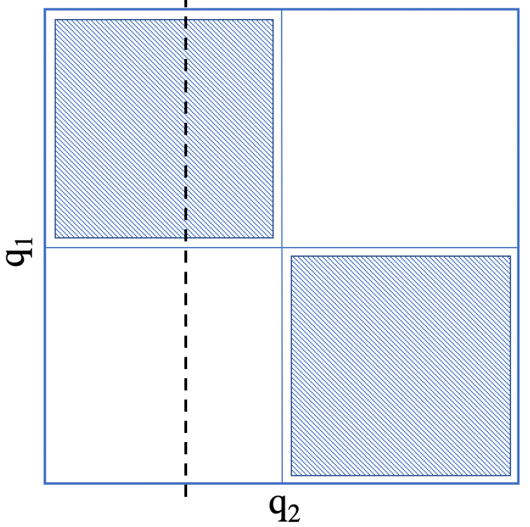
Figure 3: An example of a pattern that cannot be captured by recursive partitioning. Observations in the white and crosshatched region have different statistics. Any split, such as the black dashed line, result in two sub-partitions that have similar average statistics.

Finally, we need the following lemma for proving that the decision likelihood is increasing in each iteration in §A.1.

Lemma 1.

For any given vector $a:\sum_{i}a_{i}=1$, the answer to the following maximization problem is equal to $a$.

$$\max_{b} \quad f(b)=\sum_{i}a_{i}\ln{b_{i}}$$

s.t. $$\quad\sum_{i}b_{i}=1$$

Proof.

It is a constrained optimization problem that can be solved by maximizing the Lagrangian function.

$$\mathcal{L}(a,b,\lambda) =\sum_{i}a_{i}\ln{b_{i}}-\lambda(\sum_{i}b_{i}-1)$$

$$\nabla\mathcal{L}(b,\lambda) =0$$

$$\frac{\partial\mathcal{L}}{\partial b_{i}} =\frac{a_{i}}{b_{i}}-\lambda=0\Rightarrow a_{i}=\lambda b_{i}\Rightarrow\sum a_{i}=\lambda\sum b_{i}$$

$$\frac{\partial\mathcal{L}}{\partial\lambda} =\sum_{i}b_{i}-1=0\Rightarrow\sum_{i}b_{i}=1$$

$$\Rightarrow\lambda=1\Rightarrow b_{i}=a_{i}$$

∎

A.1 The proof of likelihood increase

In this section, we prove that the likelihood function $\operatorname{\mathcal{L}}(\theta^{*}_{r},\operatorname{\mathbf{\Pi}}_{r})$ increases at each iteration of our recursive partitioning algorithm. Formally, we prove

$$\operatorname{\mathcal{L}}(\theta^{*}_{r},\operatorname{\mathbf{\Pi}}_{r})\leq\operatorname{\mathcal{L}}(\theta^{*}_{r+1},\operatorname{\mathbf{\Pi}}_{r+1})$$ (26)

where $\operatorname{\mathbf{\Pi}}_{r}$ and $\operatorname{\mathbf{\Pi}}_{r+1}$ are the discretizations generated by the proposed recursive partitioning in iterations $r$ and $r+1$ respectively, $\theta^{*}_{r}=\arg\!\max_{\theta}\operatorname{\mathcal{L}}(\theta,\operatorname{\mathbf{\Pi}}_{r})$, and $\theta^{*}_{r+1}=\arg\!\max_{\theta}\operatorname{\mathcal{L}}(\theta,\operatorname{\mathbf{\Pi}}_{r+1})$.

Theorem 1.

For any candidate additional split, noted by $\{k,q,z\}$, to a discretization $\operatorname{\mathbf{\Pi}}$, where $k$ is a partition in $\operatorname{\mathbf{\Pi}}$, $q$ is a feature in $Q$, and $z$ is a value within the range of possible values for $q$ in $k$, the following inequalities hold

$$\exists\theta^{\prime}:\operatorname{\mathcal{L}}_{dc}(\theta^{*},\operatorname{\mathbf{\Pi}}) \leq\operatorname{\mathcal{L}}_{dc}(\theta^{\prime},\operatorname{\mathbf{\Pi}}^{\prime})$$ (27)

$$\operatorname{\mathcal{L}}_{st}(\operatorname{\mathbf{\Pi}}) \leq\operatorname{\mathcal{L}}_{st}(\operatorname{\mathbf{\Pi}}^{\prime})$$ (28)

where $\operatorname{\mathbf{\Pi}}^{\prime}=\operatorname{\mathbf{\Pi}}+\{k,q,z\}$ is the discretization after adding the candidate split, and $\theta^{*}=\arg\!\max_{\theta}\operatorname{\mathcal{L}}(\theta,\operatorname{\mathbf{\Pi}})$ is the optimal parameters given discretization $\operatorname{\mathbf{\Pi}}$.

We prove inequalities 27 and 28 separately. First, in Lemma 2, we create a new parameter set $\theta^{\prime}$ for the discretization $\operatorname{\mathbf{\Pi}}^{\prime}$ from $\theta^{*}$ that satisfy a certain inequality. Next we show that inequality 27 holds for the new parameter set $\theta^{\prime}$ and $\operatorname{\mathbf{\Pi}}^{\prime}$. Finally, we prove that for any two partitions $\operatorname{\mathbf{\Pi}}$ and $\operatorname{\mathbf{\Pi}}^{\prime}$ such that $\operatorname{\mathbf{\Pi}}$ is the parent of $\operatorname{\mathbf{\Pi}}^{\prime}$ the inequality 28 holds. Please note discretization $\operatorname{\mathbf{\Pi}}$ is the parent of any discretization that is created by adding additional splits to $\operatorname{\mathbf{\Pi}}$.

Lemma 2.

There is a flow utility coefficient set $\theta^{\prime}$ such that for any $x\in\operatorname{\mathbf{X}}$, $q\in\operatorname{\mathbf{Q}}$ and $j\in\operatorname{\mathbf{J}}$, the following equation holds

$$\exp{v(x,\operatorname{\mathbf{\Pi}}^{\prime}(q),j;\theta^{\prime},\operatorname{\mathbf{\Pi}}^{\prime})} =\exp{v(x,\operatorname{\mathbf{\Pi}}(q),j;\theta^{*},\operatorname{\mathbf{\Pi}})}$$

$$+\Big{[}\Pr(j|x,\operatorname{\mathbf{\Pi}}^{\prime}(q))-\Pr(j|x,\operatorname{\mathbf{\Pi}}(q))\Big{]}\exp{\bar{V}(x,\operatorname{\mathbf{\Pi}}(q);\theta^{*},\operatorname{\mathbf{\Pi}})}$$ (29)

Proof.

Using the equality $\log(a+b)=\log(a)+\log(1+b/a)$, we write equation 29 as the following

$$v(x,\operatorname{\mathbf{\Pi}}^{\prime}(q),j;\theta^{\prime},\operatorname{\mathbf{\Pi}}^{\prime}) =v(x,\operatorname{\mathbf{\Pi}}(q),j;\theta^{*},\operatorname{\mathbf{\Pi}})+\log\Big{(}1+\frac{\Pr(j|x,\operatorname{\mathbf{\Pi}}^{\prime}(q))-\Pr(j|x,\operatorname{\mathbf{\Pi}}(q))}{\frac{\exp{v(x,\Pi(q),j;\theta^{*},\operatorname{\mathbf{\Pi}})}}{\exp{\bar{V}(x,\Pi(q);\theta^{*},\operatorname{\mathbf{\Pi}})}}}\Big{)}$$

$$=v(x,\operatorname{\mathbf{\Pi}}(q),j;\theta^{*},\operatorname{\mathbf{\Pi}})+\log\Big{(}1+\frac{\Pr(j|x,\operatorname{\mathbf{\Pi}}^{\prime}(q))-\Pr(j|x,\operatorname{\mathbf{\Pi}}(q))}{\hat{p}(j|x,\operatorname{\mathbf{\Pi}}(q);\theta^{*},\operatorname{\mathbf{\Pi}})}\Big{)}$$ (30)

Using the formulation of the choice specific value function (equation 24), we can write equation 30 in term of the flow utility and expected value functions as follow

$$u(x,\operatorname{\mathbf{\Pi}}^{\prime}(q),j;\theta^{\prime},\operatorname{\mathbf{\Pi}}^{\prime}) =u(x,\operatorname{\mathbf{\Pi}}(q),j;\theta^{*},\operatorname{\mathbf{\Pi}})$$

$$+\sum_{x^{\prime}\in X}\sum_{\pi\in\operatorname{\mathbf{\Pi}}^{\prime}}\bar{V}(x^{\prime},\pi;\theta^{*},\operatorname{\mathbf{\Pi}})g(x^{\prime},\pi|x,\operatorname{\mathbf{\Pi}}(q),j)$$

$$-\sum_{x^{\prime}\in X}\sum_{\pi\in\operatorname{\mathbf{\Pi}}^{\prime}}\bar{V}(x^{\prime},\pi;\theta^{\prime},\operatorname{\mathbf{\Pi}}^{\prime})g(x^{\prime},\pi|x,\operatorname{\mathbf{\Pi}}^{\prime}(q),j)$$

$$+\log\Big{(}1+\frac{\Pr(j|x,\operatorname{\mathbf{\Pi}}^{\prime}(q))-\Pr(j|x,\operatorname{\mathbf{\Pi}}(q))}{\hat{p}(j|x,\operatorname{\mathbf{\Pi}}(q);\theta^{*},\operatorname{\mathbf{\Pi}})}\Big{)}$$ (31)

We assume a non-parametric functional form for the utility function; therefore, we can calculate a set of new utility values for each observable state $\{x,\pi\}$ based on the above equation that satisfies equation 29. However, the right-hand side of equation 31 uses $\theta^{\prime}$, which we are trying to calculate. If we want to use equation 31, we need to prove that this equation has a unique answer. Alternatively, we prove that if equation 29 holds, the value functions in the new partitioning and old partitioning are equal.

$$\bar{V} (x,\operatorname{\mathbf{\Pi}}^{\prime}(q);\theta^{\prime},\operatorname{\mathbf{\Pi}}^{\prime})$$

$$=\log\sum_{j\in\operatorname{\mathbf{J}}}\exp{v(x,\operatorname{\mathbf{\Pi}}^{\prime}(q),j;\theta^{\prime},\operatorname{\mathbf{\Pi}}^{\prime})}$$

$$=\log\sum_{j\in\operatorname{\mathbf{J}}}\Big{(}\exp{v(x,\operatorname{\mathbf{\Pi}}(q),j;\theta^{*},\operatorname{\mathbf{\Pi}})}+\big{[}\Pr(j|x,\operatorname{\mathbf{\Pi}}^{\prime}(q))-\Pr(j|x,\operatorname{\mathbf{\Pi}}(q))\big{]}\bar{V}(x,\operatorname{\mathbf{\Pi}}(q);\theta^{*},\operatorname{\mathbf{\Pi}})\Big{)}$$

$$=\log\Big{(}\sum_{j\in\operatorname{\mathbf{J}}}\exp{v(x,\operatorname{\mathbf{\Pi}}(q),j;\theta^{*},\operatorname{\mathbf{\Pi}})}+\bar{V}(x,\operatorname{\mathbf{\Pi}}(q);\theta^{*},\operatorname{\mathbf{\Pi}})\sum_{j\in\operatorname{\mathbf{J}}}\big{[}\Pr(j|x,\operatorname{\mathbf{\Pi}}^{\prime}(q))-\Pr(j|x,\operatorname{\mathbf{\Pi}}(q))\big{]}\Big{)}$$

$$=\log\sum_{j\in\operatorname{\mathbf{J}}}\exp{v(x,\operatorname{\mathbf{\Pi}}(q),j;\theta^{*},\operatorname{\mathbf{\Pi}})}$$

$$=\bar{V}(x,\operatorname{\mathbf{\Pi}}(q);\theta^{*},\operatorname{\mathbf{\Pi}})$$ (32)

where the equality from line $3^{rd}$ to line $4^{th}$ comes from $\sum_{j\in\operatorname{\mathbf{J}}}\big{[}\Pr(j|x,\operatorname{\mathbf{\Pi}}^{\prime}(q))-\Pr(j|x,\operatorname{\mathbf{\Pi}}(q))\big{]}=0$.

We can now write equation 31 as the following:

$$u(x,\operatorname{\mathbf{\Pi}}^{\prime}(q),j;\theta^{\prime},\operatorname{\mathbf{\Pi}}^{\prime}) =u(x,\operatorname{\mathbf{\Pi}}(q),j;\theta^{*},\operatorname{\mathbf{\Pi}})$$

$$+\sum_{x^{\prime}\in X}\sum_{\pi\in\operatorname{\mathbf{\Pi}}^{\prime}}\bar{V}(x^{\prime},\pi;\theta^{*},\operatorname{\mathbf{\Pi}})\big{(}g(x^{\prime},\pi|x,\operatorname{\mathbf{\Pi}}(q),j)-g(x^{\prime},\pi|x,\operatorname{\mathbf{\Pi}}^{\prime}(q),j)\big{)}$$

$$+\log\Big{(}1+\frac{\Pr(j|x,\operatorname{\mathbf{\Pi}}^{\prime}(q))-\Pr(j|x,\operatorname{\mathbf{\Pi}}(q))}{\hat{p}(j|x,\operatorname{\mathbf{\Pi}}(q);\theta^{*},\operatorname{\mathbf{\Pi}})}\Big{)}$$ (33)

This equation is not dependent on $\theta^{\prime}$, and can be used to calculate a set of utility function values ($\theta^{\prime}$) for partitioning $\operatorname{\mathbf{\Pi}}^{\prime}$. ∎

Proof of inequality 27.

We show in lemma 2 that there is a $\theta^{\prime}$ such that equality 29 holds, and for any $x\in X$ and $q\in\operatorname{\mathbf{Q}}$ we have $\bar{V}(x,\operatorname{\mathbf{\Pi}}^{\prime}(q);\theta^{\prime},\operatorname{\mathbf{\Pi}}^{\prime})=\bar{V}(x,\operatorname{\mathbf{\Pi}}(q);\theta^{*},\operatorname{\mathbf{\Pi}})$. Since $\bar{V}(.;\theta^{*},\operatorname{\mathbf{\Pi}})$ is a fixed point solution to the standard contraction mapping problem for the Bellman equation, $\bar{V}(.;\theta^{\prime},\operatorname{\mathbf{\Pi}}^{\prime})$ generated in lemma 2 is a solution to the contraction mapping in Bellman equation as well. Additionally, we have

$$\operatorname{\mathcal{L}}_{dc}(\theta^{\prime},\operatorname{\mathbf{\Pi}}^{\prime}) =\sum_{i=1}^{N}\sum_{t=1}^{T}\log\hat{p}(d_{it}|x_{it},\operatorname{\mathbf{\Pi}}^{\prime}(q_{it});\theta^{\prime},\operatorname{\mathbf{\Pi}}^{\prime})$$

$$=\sum_{i=1}^{N}\sum_{t=1}^{T}\log\frac{\exp{v(x_{it},\operatorname{\mathbf{\Pi}}(q_{it}),d_{it};\theta^{\prime},\operatorname{\mathbf{\Pi}}^{\prime})}}{\exp{\bar{V}(x_{it},\operatorname{\mathbf{\Pi}}(q_{it});\theta^{\prime},\operatorname{\mathbf{\Pi}}^{\prime})}}$$

$$=\sum_{i=1}^{N}\sum_{t=1}^{T}\log\frac{\exp{v(x_{it},\operatorname{\mathbf{\Pi}}(q_{it}),d_{it};\theta^{\prime},\operatorname{\mathbf{\Pi}}^{\prime})}}{\exp{\bar{V}(x_{it},\operatorname{\mathbf{\Pi}}(q_{it});\theta^{*},\operatorname{\mathbf{\Pi}})}}$$

$$=\sum_{i=1}^{N}\sum_{t=1}^{T}\log\Big{(}\frac{\exp{v(x_{it},\operatorname{\mathbf{\Pi}}(q_{it}),d_{it};\theta^{*},\operatorname{\mathbf{\Pi}})}}{\exp{\bar{V}(x_{it},\operatorname{\mathbf{\Pi}}(q_{it});\theta^{*},\operatorname{\mathbf{\Pi}})}}+\Pr(d_{it}|x_{it},\operatorname{\mathbf{\Pi}}^{\prime}(q_{it}))-\Pr(d_{it}|x_{it},\operatorname{\mathbf{\Pi}}(q_{it}))\Big{)}$$ (34)

Please note the equality between line two and line three is driven from equation 32, and between line three and line four from equation 29. Using $\log(a+b)=\log(a)+\log(1+b/a)$, we have the following

$$\operatorname{\mathcal{L}}_{dc}(\theta^{\prime},\operatorname{\mathbf{\Pi}}^{\prime})=\sum_{i=1}^{N}\sum_{t=1}^{T}\log\Big{(}\frac{\exp{v(x_{it},\operatorname{\mathbf{\Pi}}(q_{it}),d_{it};\theta^{*},\operatorname{\mathbf{\Pi}})}}{\exp{\bar{V}(x_{it},\operatorname{\mathbf{\Pi}}(q_{it});\theta^{*},\operatorname{\mathbf{\Pi}})}}+\Pr(d_{it}|x_{it},\operatorname{\mathbf{\Pi}}^{\prime}(q_{it}))-\Pr(d_{it}|x_{it},\operatorname{\mathbf{\Pi}}(q_{it}))\Big{)}$$

$$=\sum_{i=1}^{N}\sum_{t=1}^{T}\log\Big{(}\frac{\exp{v(x_{it},\operatorname{\mathbf{\Pi}}(q_{it}),d_{it};\theta^{*},\operatorname{\mathbf{\Pi}})}}{\exp{\bar{V}(x_{it},\operatorname{\mathbf{\Pi}}(q_{it});\theta^{*},\operatorname{\mathbf{\Pi}})}}\Big{)}+\sum_{i=1}^{N}\sum_{t=1}^{T}\log\Big{(}1+\frac{\Pr(d_{it}|x_{it},\operatorname{\mathbf{\Pi}}^{\prime}(q_{it}))-\Pr(d_{it}|x_{it},\operatorname{\mathbf{\Pi}}(q_{it}))}{\frac{\exp{v(x_{it},\operatorname{\mathbf{\Pi}}(q_{it}),d_{it};\theta^{*},\operatorname{\mathbf{\Pi}})}}{\exp{\bar{V}(x_{it},\operatorname{\mathbf{\Pi}}(q_{it});\theta^{*},\operatorname{\mathbf{\Pi}})}}}\Big{)}$$

$$=\operatorname{\mathcal{L}}_{dc}(\theta^{*},\operatorname{\mathbf{\Pi}})+\sum_{i=1}^{N}\sum_{t=1}^{T}\log\Big{(}1+\frac{\Pr(d_{it}|x_{it},\operatorname{\mathbf{\Pi}}^{\prime}(q_{it}))-\Pr(d_{it}|x_{it},\operatorname{\mathbf{\Pi}}(q_{it}))}{\hat{p}(d_{it}|x_{it},\operatorname{\mathbf{\Pi}}(q_{it});\theta^{*},\operatorname{\mathbf{\Pi}})}\Big{)}$$

$$\Rightarrow\operatorname{\mathcal{L}}_{dc}(\theta^{\prime},\operatorname{\mathbf{\Pi}}^{\prime})-\operatorname{\mathcal{L}}_{dc}(\theta^{*},\operatorname{\mathbf{\Pi}})=\sum_{i=1}^{N}\sum_{t=1}^{T}\log\Big{(}1+\frac{\Pr(d_{it}|x_{it},\operatorname{\mathbf{\Pi}}^{\prime}(q_{it}))-\Pr(d_{it}|x_{it},\operatorname{\mathbf{\Pi}}(q_{it}))}{\hat{p}(d_{it}|x_{it},\operatorname{\mathbf{\Pi}}(q_{it});\theta^{*},\operatorname{\mathbf{\Pi}})}\Big{)}$$ (35)

We will show that the right-hand side of equation 35 is positive; thus, proving that the likelihood is increasing. Assuming $NT\to\infty$, and our predicted choice probabilities are consistent, concludes $\hat{p}(d_{it}|x_{it},\operatorname{\mathbf{\Pi}}(q_{it});\theta^{*},\operatorname{\mathbf{\Pi}})=\Pr(d_{it}|x_{it},\operatorname{\mathbf{\Pi}}(q_{it}))$. Replacing the predicted choice probability with its counter-part conditional choice probability in equation 35 yields

$$\sum_{i=1}^{N}\sum_{t=1}^{T}\log\Big{(}1+\frac{\Pr(d_{it}|x_{it},\operatorname{\mathbf{\Pi}}^{\prime}(q_{it}))-\Pr(d_{it}|x_{it},\operatorname{\mathbf{\Pi}}(q_{it}))}{\hat{p}(d_{it}|x_{it},\operatorname{\mathbf{\Pi}}(q_{it});\theta^{*},\operatorname{\mathbf{\Pi}})}\Big{)}$$

$$=\sum_{i=1}^{N}\sum_{t=1}^{T}\log\Big{(}1+\frac{\Pr(d_{it}|x_{it},\operatorname{\mathbf{\Pi}}^{\prime}(q_{it}))-\Pr(d_{it}|x_{it},\operatorname{\mathbf{\Pi}}(q_{it}))}{\Pr(d_{it}|x_{it},\operatorname{\mathbf{\Pi}}(q_{it}))}\Big{)}$$

$$=\sum_{i=1}^{N}\sum_{t=1}^{T}\log\frac{\Pr(d_{it}|x_{it},\operatorname{\mathbf{\Pi}}^{\prime}(q_{it}))}{\Pr(d_{it}|x_{it},\operatorname{\mathbf{\Pi}}(q_{it}))}$$ (36)

The value inside the summation in equation 36 is equal to zero for all the observations, except for those where $q_{it}$ lands in the newly split partition. Let us call the partition before the split $\pi_{p}\in\operatorname{\mathbf{\Pi}}$, and the two resulting partitions $\{\pi_{l},\pi_{r}\}\in\operatorname{\mathbf{\Pi}}^{\prime}$. Also let $N(x,\pi)$ denote the number of observations where $x_{it}=x$ and $\operatorname{\mathbf{\Pi}}^{\prime}(q_{it})=\pi$, and $N(x,\pi,j)$ denote the number where in addition to the aforementioned conditions $d_{it}=j$. We can write 36 as follow:

$$\sum_{i=1}^{N}\sum_{t=1}^{T} \log\frac{\Pr(d_{it}|x_{it},\operatorname{\mathbf{\Pi}}^{\prime}(q_{it}))}{\Pr(d_{it}|x_{it},\operatorname{\mathbf{\Pi}}(q_{it}))}=\sum_{x\in X}\sum_{\pi\in\{\pi_{l},\pi_{r}\}}\sum_{j\in\operatorname{\mathbf{J}}}N(x,\pi,j)\log\big{(}\Pr(j|x,\pi)-\Pr(j|x,\pi_{p})\big{)}$$

$$=\sum_{x\in X}\sum_{\pi\in\{\pi_{l},\pi_{r}\}}N(x,\pi)\sum_{j\in\operatorname{\mathbf{J}}}\big{(}\Pr(j|x,\pi)\log\Pr(j|x,\pi)-\Pr(j|x,\pi)\log\Pr(j|x,\pi_{p})\big{)}$$

According to Lemma 1, $\sum_{j\in\operatorname{\mathbf{J}}}\Pr(j|x,\pi)\log\Pr(j|x,\pi)\geq\sum_{j\in\operatorname{\mathbf{J}}}\Pr(j|x,\pi)\log\Pr(j|x,\pi_{p})$. This inequality is strict if there is a $j\in\operatorname{\mathbf{J}}$ such that $\Pr(j|x,\pi)\neq\Pr(j|x,\pi_{p})$ for any $x\in X$ and $\pi\in\{\pi_{l},\pi_{r}\}$. Thus, equation 36 is greater or equal than zero, which proves the inequality 27 in theorem 1. ∎

Proof of inequality 28.

First note that discretization $\operatorname{\mathbf{\Pi}}$ is a parent of discretization $\operatorname{\mathbf{\Pi}}^{\prime}$. Based on the definition of parent, for every $\pi\in\operatorname{\mathbf{\Pi}}$, there is a set of partitions $\{\pi_{i}\}\in\operatorname{\mathbf{\Pi}}^{\prime}$ such that $\bigcup\limits_{i}\pi_{i}=\pi$. Let us call $\{\pi_{i}\}$ the child set of $\pi$ in $\operatorname{\mathbf{\Pi}}^{\prime}$ and denote it by $\operatorname{\mathbf{\Pi}}^{\prime}(\pi)$. First we use the log sum inequality (Cover and Thomas, 1991) to prove that for any $\{\pi,\pi^{\prime}\}\in\operatorname{\mathbf{\Pi}}$, $\{x,x^{\prime}\}\in\operatorname{\mathbf{X}}$ , and $j\in\operatorname{\mathbf{J}}$ the following inequality holds

$$\sum_{\pi_{i}\in\operatorname{\mathbf{\Pi}}^{\prime}(\pi)}\sum_{\pi^{\prime}_{i}\in\operatorname{\mathbf{\Pi}}^{\prime}(\pi^{\prime})}N(x,\pi_{i},x^{\prime},\pi^{\prime}_{i},j)\log\frac{N(x,\pi_{i},x^{\prime},\pi^{\prime}_{i},j)}{N(x,\pi_{i})N(x^{\prime},\pi^{\prime}_{i},j)}\geq N(x,\pi,x^{\prime},\pi^{\prime},j)\log\frac{N(x,\pi,x^{\prime},\pi^{\prime},j)}{N(x,\pi)N(x^{\prime},\pi^{\prime},j)}$$ (37)

We prove this inequality by applying the log sum inequality twice. First for a given $\pi_{i}\in\operatorname{\mathbf{\Pi}}^{\prime}(\pi)$ the following holds according to log sum inequality.

$$\sum_{\pi^{\prime}_{i}\in\operatorname{\mathbf{\Pi}}^{\prime}(\pi^{\prime})}N(x,\pi_{i},x^{\prime},\pi^{\prime}_{i},j)\log\frac{N(x,\pi_{i},x^{\prime},\pi^{\prime}_{i},j)}{N(x^{\prime},\pi^{\prime}_{i},j)}\geq N(x,\pi_{i},x^{\prime},\pi^{\prime},j)\log\frac{N(x,\pi_{i},x^{\prime},\pi^{\prime},j)}{N(x^{\prime},\pi^{\prime},j)}$$ (38)

which by subtracting $N(x,\pi_{i},x^{\prime},\pi^{\prime},j)\log N(x,\pi_{i})$ from both sides changes to

$$\sum_{\pi^{\prime}_{i}\in\operatorname{\mathbf{\Pi}}^{\prime}(\pi^{\prime})}N(x,\pi_{i},x^{\prime},\pi^{\prime}_{i},j)\log\frac{N(x,\pi_{i},x^{\prime},\pi^{\prime}_{i},j)}{N(x^{\prime},\pi^{\prime}_{i},j)N(x,\pi_{i})}\geq N(x,\pi_{i},x^{\prime},\pi^{\prime},j)\log\frac{N(x,\pi_{i},x^{\prime},\pi^{\prime},j)}{N(x^{\prime},\pi^{\prime},j)N(x,\pi_{i})}.$$ (39)

Similarly, according to log sum inequality we have

$$\sum_{\pi_{i}\in\operatorname{\mathbf{\Pi}}^{\prime}(\pi)}N(x,\pi_{i},x^{\prime},\pi^{\prime},j)\log\frac{N(x,\pi_{i},x^{\prime},\pi^{\prime},j)}{N(x,\pi_{i})}\geq N(x,\pi,x^{\prime},\pi^{\prime},j)\log\frac{N(x,\pi,x^{\prime},\pi^{\prime},j)}{N(x,\pi)}$$ (40)

which by subtracting $N(x,\pi,x^{\prime},\pi^{\prime},j)\log N(x^{\prime},\pi^{\prime},j)$ from both sides changes to

$$\sum_{\pi_{i}\in\operatorname{\mathbf{\Pi}}^{\prime}(\pi)}N(x,\pi_{i},x^{\prime},\pi^{\prime},j)\log\frac{N(x,\pi_{i},x^{\prime},\pi^{\prime},j)}{N(x,\pi_{i})N(x^{\prime},\pi^{\prime},j)}\geq N(x,\pi,x^{\prime},\pi^{\prime},j)\log\frac{N(x,\pi,x^{\prime},\pi^{\prime},j)}{N(x,\pi)N(x^{\prime},\pi^{\prime},j)}.$$ (41)

By merging inequalities 39 and 41 we have

$$\sum_{\pi_{i}\in\operatorname{\mathbf{\Pi}}^{\prime}(\pi)}\sum_{\pi^{\prime}_{i}\in\operatorname{\mathbf{\Pi}}^{\prime}(\pi^{\prime})} N(x,\pi_{i},x^{\prime},\pi^{\prime}_{i},j)\log\frac{N(x,\pi_{i},x^{\prime},\pi^{\prime}_{i},j)}{N(x,\pi_{i})N(x^{\prime},\pi^{\prime}_{i},j)}$$

$$\geq\sum_{\pi_{i}\in\operatorname{\mathbf{\Pi}}^{\prime}(\pi)}N(x,\pi_{i},x^{\prime},\pi^{\prime},j)\log\frac{N(x,\pi_{i},x^{\prime},\pi^{\prime},j)}{N(x,\pi_{i})N(x^{\prime},\pi^{\prime},j)}$$

$$\geq N(x,\pi,x^{\prime},\pi^{\prime},j)\log\frac{N(x,\pi,x^{\prime},\pi^{\prime},j)}{N(x,\pi)N(x^{\prime},\pi^{\prime},j)}$$

which concludes inequality 37. We can prove the lemma by summing this inequality over all $\{\pi,\pi^{\prime}\}\in\operatorname{\mathbf{\Pi}}$, $\{x,x^{\prime}\}\in\operatorname{\mathbf{X}}$ and $j\in\operatorname{\mathbf{J}}$. ∎

We proved both inequalities in the theorem 1. Next we prove that the equality happens if and only if our algorithm reaches a perfect discretization.

A.2 The proof of convergence to perfect discretization

In this section we prove that our proposed algorithm stops once it reaches a perfect discretization.

Theorem 2.

The recursive partitioning algorithm discussed in $\S$4 stops once it find a perfect discretization, i.e., $\operatorname{\mathcal{F}}(\operatorname{\mathbf{\Pi}}_{r})=\operatorname{\mathcal{F}}(\operatorname{\mathbf{\Pi}}_{r+1})$ if and only if $\operatorname{\mathbf{\Pi}}_{r}$ is a perfect discretization.

We prove this theorem by proving separate lemmas for decision and state transition probabilities. Let us denote the decision and transition part of $\operatorname{\mathcal{F}}(\operatorname{\mathbf{\Pi}})$ by $\operatorname{\mathcal{F}}_{dc}(\operatorname{\mathbf{\Pi}})$ and $\operatorname{\mathcal{F}}_{tr}(\operatorname{\mathbf{\Pi}})$ respectively.

Lemma 3.

For any candidate additional split $\{k,q,z\}$ to discretization $\operatorname{\mathbf{\Pi}}$, that splits $\pi_{p}\in\operatorname{\mathbf{\Pi}}$ into $\{\pi_{l},\pi_{r}\}\in\operatorname{\mathbf{\Pi}}^{\prime}$, we have $\operatorname{\mathcal{F}}_{dc}(\operatorname{\mathbf{\Pi}})=\operatorname{\mathcal{F}}_{dc}(\operatorname{\mathbf{\Pi}}^{\prime})$ if and only if for all $x\in\operatorname{\mathbf{X}}$ and $j\in\operatorname{\mathbf{J}}$ the decision probabilities in $\pi_{l}$ and $\pi_{r}$ are similar, i.e., $\Pr(j|x,\pi_{l})=\Pr(j|x,\pi_{r})$.

Proof.

We have

$$\operatorname{\mathcal{F}}_{dc}(\operatorname{\mathbf{\Pi}}^{\prime})-\operatorname{\mathcal{F}}_{dc}(\operatorname{\mathbf{\Pi}}) =N(x,\pi_{l},j;\operatorname{\mathbf{\Pi}})\log\frac{N(x,\pi_{l},j;\operatorname{\mathbf{\Pi}})}{N(x,\pi_{l};\operatorname{\mathbf{\Pi}})}+N(x,\pi_{r},j;\operatorname{\mathbf{\Pi}})\log\frac{N(x,\pi_{r},j;\operatorname{\mathbf{\Pi}})}{N(x,\pi_{r};\operatorname{\mathbf{\Pi}})}$$

$$-N(x,\pi_{p},j;\operatorname{\mathbf{\Pi}})\log\frac{N(x,\pi_{p},j;\operatorname{\mathbf{\Pi}})}{N(x,\pi_{p};\operatorname{\mathbf{\Pi}})}$$

According to log sum inequality the right-hand side of this equality is equal to zero if and only if $\frac{N(x,\pi_{r},j;\operatorname{\mathbf{\Pi}})}{N(x,\pi_{r};\operatorname{\mathbf{\Pi}})}=\frac{N(x,\pi_{l},j;\operatorname{\mathbf{\Pi}})}{N(x,\pi_{l};\operatorname{\mathbf{\Pi}})}$, which concludes $\Pr(j|x,\pi_{l})=\Pr(j|x,\pi_{r})$. ∎

Lemma 4.

For any candidate additional split $\{k,q,z\}$ to discretization $\operatorname{\mathbf{\Pi}}$, that splits $\pi_{p}\in\operatorname{\mathbf{\Pi}}$ into $\{\pi_{l},\pi_{r}\}\in\operatorname{\mathbf{\Pi}}^{\prime}$, we have $\operatorname{\mathcal{F}}_{tr}(\operatorname{\mathbf{\Pi}})=\operatorname{\mathcal{F}}_{tr}(\operatorname{\mathbf{\Pi}}^{\prime})$ if and only if for all $\{x,x^{\prime}\}\in\operatorname{\mathbf{X}}$, $\pi^{\prime}\in\operatorname{\mathbf{\Pi}}^{\prime}$, and $j\in\operatorname{\mathbf{J}}$ the following equations hold

$$\Pr(x^{\prime},\pi^{\prime}|x,\pi_{l},j) =\Pr(x^{\prime},\pi^{\prime}|x,\pi_{r},j)$$

$$\frac{\Pr(x,\pi_{l}|x^{\prime},\pi^{\prime},j)}{N(x,\pi_{l})} =\frac{\Pr(x,\pi_{r}|x^{\prime},\pi^{\prime},j)}{N(x,\pi_{r})}$$

Proof.

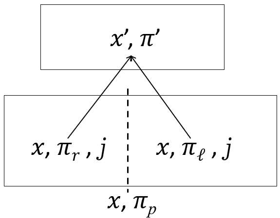
(a) Transition from the new sub-partitions

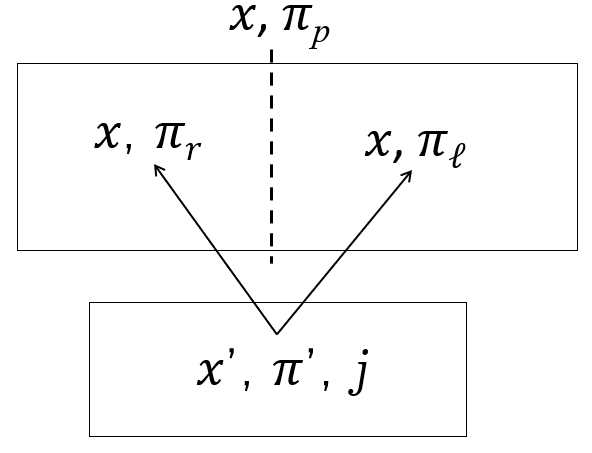
(b) Transition to the new sub-partitions

Figure 4: The change in likelihood from transition-to and transition-from perspective.

We proved in appendix A.1 that likelihood, $\operatorname{\mathcal{L}}(\theta_{t})$, increases with any additional split. We assumed a completely non-parametric form for the state transition part of likelihood function. Therefore the state transition of likelihood function and recursive partitioning objective function are the same, i.e., $\operatorname{\mathcal{L}}_{tr}(\operatorname{\mathbf{\Pi}})=\operatorname{\mathcal{F}}_{tr}(\operatorname{\mathbf{\Pi}})$. Here we prove that the increment in likelihood, and consequently in $\operatorname{\mathcal{F}}(\theta_{t})$, is equal to zero if and only if the lemma’s equations hold. The split changes the likelihood by changing the transition-to and average transition-from probabilities presented in figure 4. We can calculate the changes in likelihood with respect to each of these changes separately. First, according to (a) in figure 4 we have

$$\operatorname{\mathcal{F}}(\operatorname{\mathbf{\Pi}}^{\prime})-\operatorname{\mathcal{F}}(\operatorname{\mathbf{\Pi}})=\sum_{x,x^{\prime}\in\operatorname{\mathbf{X}}}\sum_{\pi^{\prime}\in\operatorname{\mathbf{\Pi}}^{\prime}}\sum_{j\in\operatorname{\mathbf{J}}}N(x^{\prime},\pi^{\prime})\Bigg{(} \frac{N(x^{\prime},\pi^{\prime},x,\pi_{r},j)}{N(x^{\prime},\pi^{\prime})}\log\frac{N(x^{\prime},\pi^{\prime},x,\pi_{r},j)}{N(x^{\prime},\pi^{\prime})N(x,\pi_{r},j)}$$

$$+ \frac{N(x^{\prime},\pi^{\prime},x,\pi_{l},j)}{N(x^{\prime},\pi^{\prime})}\log\frac{N(x^{\prime},\pi^{\prime},x,\pi_{l},j)}{N(x^{\prime},\pi^{\prime})N(x,\pi_{l},j)}$$

$$- \frac{N(x^{\prime},\pi^{\prime},x,\pi_{p},j)}{N(x^{\prime},\pi^{\prime})}\log\frac{N(x^{\prime},\pi^{\prime},x,\pi_{p},j)}{N(x^{\prime},\pi^{\prime})N(x,\pi_{p},j)}\Bigg{)}$$

According to log sum inequality the term in the parentheses is greater or equal to zero. The left-hand side is equal to zero if and only if $\frac{N(x^{\prime},\pi^{\prime},x,\pi_{l},j)}{N(x,\pi_{l},j)}=\frac{N(x^{\prime},\pi^{\prime},x,\pi_{r},j)}{N(x,\pi_{r},j)}=\frac{N(x^{\prime},\pi^{\prime},x,\pi_{p},j)}{N(x,\pi_{p},j)}$, for every $\{x,x^{\prime}\}\in\operatorname{\mathbf{X}}$, $j\in\operatorname{\mathbf{J}}$ and $\pi^{\prime}\in\operatorname{\mathbf{\Pi}}^{\prime}$. This concludes the first equation of the lemma.

We can conclude the second equation similarly with (b) in figure 4 as the following

$$\operatorname{\mathcal{F}}(\operatorname{\mathbf{\Pi}}^{\prime})-\operatorname{\mathcal{F}}(\operatorname{\mathbf{\Pi}})=\sum_{x,x^{\prime}\in\operatorname{\mathbf{X}}}\sum_{\pi^{\prime}\in\operatorname{\mathbf{\Pi}}^{\prime}}\sum_{j\in\operatorname{\mathbf{J}}}N(x^{\prime},\pi^{\prime},j)\Bigg{(} \frac{N(x,\pi_{r},x^{\prime},\pi^{\prime},j)}{N(x^{\prime},\pi^{\prime},j)}\log\frac{N(x,\pi_{r},x^{\prime},\pi^{\prime},j)}{N(x,\pi_{r})N(x^{\prime},\pi^{\prime},j)}$$

$$+ \frac{N(x,\pi_{l},x^{\prime},\pi^{\prime},j)}{N(x^{\prime},\pi^{\prime},j)}\log\frac{N(x,\pi_{l},x^{\prime},\pi^{\prime},j)}{N(x,\pi_{l})N(x^{\prime},\pi^{\prime},j)}$$

$$- \frac{N(x,\pi_{p},x^{\prime},\pi^{\prime},j)}{N(x^{\prime},\pi^{\prime},j)}\log\frac{N(x,\pi_{p},x^{\prime},\pi^{\prime},j)}{N(x,\pi_{p})N(x^{\prime},\pi^{\prime},j)}\Bigg{)}$$

Again, according to log sum inequality the term in the parentheses is greater or equal to zero. The left-hand side is equal to zero if and only if $\frac{N(x^{\prime},\pi^{\prime},x,\pi_{l},j)}{N(x,\pi_{l})N(x^{\prime},\pi^{\prime},j)}=\frac{N(x^{\prime},\pi^{\prime},x,\pi_{r},j)}{N(x,\pi_{r})N(x^{\prime},\pi^{\prime},j)}=\frac{N(x^{\prime},\pi^{\prime},x,\pi_{p},j)}{N(x,\pi_{p})N(x^{\prime},\pi^{\prime},j)}$, for every $\{x,x^{\prime}\}\in\operatorname{\mathbf{X}}$, $j\in\operatorname{\mathbf{J}}$ and $\pi^{\prime}\in\operatorname{\mathbf{\Pi}}^{\prime}$. This concludes the second equation of the lemma. ∎

Proof for theorem 2.

Now we prove theorem 2 using lemmas 4 and 3. Assume that our algorithm stops at iteration $r$. Given that the algorithm stops once no split increase the $\operatorname{\mathcal{F}}$ function, for any additional split that generates candidate partition $\operatorname{\mathbf{\Pi}}^{\prime}$, we have $\operatorname{\mathcal{F}}(\operatorname{\mathbf{\Pi}}^{\prime})=\operatorname{\mathcal{F}}(\operatorname{\mathbf{\Pi}}_{r})$. Therefore, according to lemmas 4 and 3 for any additional split to $\operatorname{\mathbf{\Pi}}_{r}$ the following equalities hold for all $\{x,x^{\prime}\}\in\operatorname{\mathbf{X}}$, $\pi^{\prime}\in\operatorname{\mathbf{\Pi}}_{r}$ and $j\in\operatorname{\mathbf{J}}$.

$$\Pr(d|x,\pi_{l}) =\Pr(d|x,\pi_{r})$$

$$\Pr(x^{\prime},\pi^{\prime}|x,\pi_{l},j) =\Pr(x^{\prime},\pi^{\prime}|x,\pi_{r},j)$$

$$\frac{\Pr(x,\pi_{l}|x^{\prime},\pi^{\prime},j)}{N(x,\pi_{l})} =\frac{\Pr(x,\pi_{r}|x^{\prime},\pi^{\prime},j)}{N(x,\pi_{r})}$$

which concludes that $\operatorname{\mathbf{\Pi}}_{r}$ is a perfect discretization according to corollary 1. ∎

Appendix B Random discretization generator algorithm

This section explains the random discretization generator algorithm that we used in the second simulation study. The intuition for this algorithm is very similar to recursive partitioning – in each step, we randomly select one of the partitions and split it into two partitions along one of the first 10 variables in $\operatorname{\mathbf{Q}}$. Please note that we only used the first 10 variables in $\operatorname{\mathbf{Q}}$ for partitioning, and the following 20 variables are added as irrelevant variables to show the robustness of the algorithm to irrelevant variables. In addition, to prevent very small or very large partitions, the random partition selection is weighted by the size of the partition: big partitions are more likely to be selected than smaller partitions. Formally, the random partitioning algorithm is as the following.

• Initialize $\operatorname{\mathbf{\Pi}}_{0}$ as one partition equal to the full covariate space

• Do the following for 15 rounds.

  • Randomly select a partition from $\operatorname{\mathbf{\Pi}}_{r}$ weighted by $(\frac{1}{\text{partition's total splits}})^{2}$

  • Randomly select a variable from the first 10 variables

  • If possible, split the selected partition into two from the midpoint along the selected variable. The total split for the resulting partitions is the total split of their parents plus one. Repeat this round if the split is not possible.

The total split for each partition is the total of times their parents have selected to be split. If the total split for a partition is 5, it means that it takes five splits from $\operatorname{\mathbf{Q}}$ to get to that partition. Note that the total split of a partition is negatively correlated with the size of the partition.

We also vary the replacement cost for each partition to add a decision variation to the model that is not caused by state transition. The replacement cost of a partition is calculated based on the range of its first 10 variables as the following.

$$f_{dc}(\pi)=5-\frac{\sum_{i=1}^{10}(v_{i}^{min}(\pi)+v_{i}^{max}(\pi))}{10}$$

where $v_{i}^{min}(\pi)$ and $v_{i}^{max}(\pi)$ are the minimum and maximum range of $i^{th}$ variable in partition $\pi$. We choose this formulation for replacement cost to create a good balance between decision variation caused by state transition or replacement cost. Figure 5 depicts the distribution of total split and replacement costs in the 1500 generated partitions across all the 100 generated discretizations in the second simulation study.

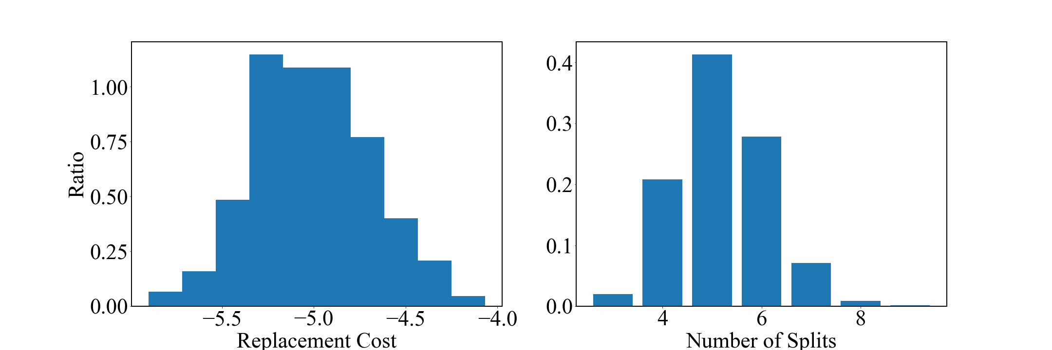
Figure 5: The histogram of generated partitions’ calculated replacement cost, and number of splits in the 100 rounds of partitioning generation.

References

- Aguirregabiria and Mira (2002) V. Aguirregabiria and P. Mira. Swapping the nested fixed point algorithm: A class of estimators for discrete markov decision models. Econometrica, 70(4):1519–1543, 2002.
- Arcidiacono and Jones (2003) P. Arcidiacono and J. B. Jones. Finite mixture distributions, sequential likelihood and the em algorithm. Econometrica, 71(3):933–946, 2003.
- Arcidiacono and Miller (2011) P. Arcidiacono and R. A. Miller. Conditional choice probability estimation of dynamic discrete choice models with unobserved heterogeneity. Econometrica, 79(6):1823–1867, 2011.
- Arcidiacono et al. (2012) P. Arcidiacono, P. Bayer, F. A. Bugni, and J. James. Approximating high-dimensional dynamic models: Sieve value function iteration. Technical report, National Bureau of Economic Research, 2012.
- Arcidiacono et al. (2013) P. Arcidiacono, P. Bayer, F. A. Bugni, and J. James. Approximating high-dimensional dynamic models: Sieve value function iteration. Emerald Group Publishing Limited, 2013.
- Athey and Imbens (2016) S. Athey and G. Imbens. Recursive partitioning for heterogeneous causal effects. Proceedings of the National Academy of Sciences, 113(27):7353–7360, 2016.
- Athey et al. (2019) S. Athey, J. Tibshirani, S. Wager, et al. Generalized random forests. The Annals of Statistics, 47(2):1148–1178, 2019.
- Benitez-Silva et al. (2000) H. Benitez-Silva, G. Hall, G. J. Hitsch, G. Pauletto, and J. Rust. A comparison of discrete and parametric approximation methods for continuous-state dynamic programming problems. manuscript, Yale University, 2000.
- Biau et al. (2008) G. Biau, L. Devroye, and G. Lugosi. Consistency of random forests and other averaging classifiers. Journal of Machine Learning Research, 9(Sep):2015–2033, 2008.
- Breiman (2001) L. Breiman. Random forests. Machine learning, 45(1):5–32, 2001.
- Breiman et al. (1984) L. Breiman, J. Friedman, C. J. Stone, and R. A. Olshen. Classification and regression trees. CRC press, 1984.
- Chen and Goodman (1999) S. F. Chen and J. Goodman. An empirical study of smoothing techniques for language modeling. Computer Speech & Language, 13(4):359–394, 1999.
- Chen and Guestrin (2016) T. Chen and C. Guestrin. Xgboost: A scalable tree boosting system. In Proceedings of the 22nd acm sigkdd international conference on knowledge discovery and data mining, pages 785–794, 2016.
- Cover and Thomas (1991) T. M. Cover and J. A. Thomas. Entropy, relative entropy and mutual information. Elements of information theory, 2:1–55, 1991.
- Dubé et al. (2012) J.-P. Dubé, J. T. Fox, and C.-L. Su. Improving the numerical performance of static and dynamic aggregate discrete choice random coefficients demand estimation. Econometrica, 80(5):2231–2267, 2012.
- Hastie et al. (2009) T. Hastie, R. Tibshirani, and J. Friedman. The elements of statistical learnin. Cited on, page 33, 2009.
- Hotz and Miller (1993) V. J. Hotz and R. A. Miller. Conditional choice probabilities and the estimation of dynamic models. The Review of Economic Studies, 60(3):497–529, 1993.
- Hotz et al. (1994) V. J. Hotz, R. A. Miller, S. Sanders, and J. Smith. A simulation estimator for dynamic models of discrete choice. The Review of Economic Studies, 61(2):265–289, 1994.
- Johnson (1932) W. E. Johnson. Probability: The deductive and inductive problems. Mind, 41(164):409–423, 1932.
- Keane and Wolpin (1994) M. P. Keane and K. I. Wolpin. The solution and estimation of discrete choice dynamic programming models by simulation and interpolation: Monte carlo evidence. the Review of economics and statistics, pages 648–672, 1994.
- Norets (2012) A. Norets. Estimation of dynamic discrete choice models using artificial neural network approximations. Econometric Reviews, 31(1):84–106, 2012.
- Powell (2007) W. Powell. Approximate Dynamic Programming: Solving the Curses of Dimensionality. Wiley Series in Probability and Statistics. Wiley, 2007. ISBN 9780470182956. URL https://books.google.com/books?id=WWWDkd65TdYC.
- Rust (1987) J. Rust. Optimal replacement of gmc bus engines: An empirical model of harold zurcher. Econometrica: Journal of the Econometric Society, pages 999–1033, 1987.
- Rust (1997) J. Rust. Using randomization to break the curse of dimensionality. Econometrica: Journal of the Econometric Society, pages 487–516, 1997.
- Rust (2000) J. Rust. Parametric policy iteration: An efficient algorithm for solving multidimensional dp problems? Technical report, Mimeo, Yale University, 2000.
- Sani et al. (2018) H. M. Sani, C. Lei, and D. Neagu. Computational complexity analysis of decision tree algorithms. In International Conference on Innovative Techniques and Applications of Artificial Intelligence, pages 191–197. Springer, 2018.
- Semenova (2018) V. Semenova. Machine learning for dynamic discrete choice. arXiv preprint arXiv:1808.02569, 2018.
- Smammut and Webb (2010) C. Smammut and G. I. Webb, editors. Bellman Equation, pages 97–97. Springer US, Boston, MA, 2010. ISBN 978-0-387-30164-8. doi: 10.1007/978-0-387-30164-8˙71. URL https://doi.org/10.1007/978-0-387-30164-8_71.
- Su and Judd (2012) C.-L. Su and K. L. Judd. Constrained optimization approaches to estimation of structural models. Econometrica, 80(5):2213–2230, 2012.
- Wu (1983) C. J. Wu. On the convergence properties of the em algorithm. The Annals of statistics, pages 95–103, 1983.
- Zimek et al. (2012) A. Zimek, E. Schubert, and H.-P. Kriegel. A survey on unsupervised outlier detection in high-dimensional numerical data. Statistical Analysis and Data Mining: The ASA Data Science Journal, 5(5):363–387, 2012.