Mitigating Smart Jammers in Multi-User MIMO

Abstract

Wireless systems must be resilient to jamming attacks. Existing mitigation methods based on multi-antenna processing require knowledge of the jammer’s transmit characteristics that may be difficult to acquire, especially for smart jammers that evade mitigation by transmitting only at specific instants. We propose a novel method to mitigate smart jamming attacks on the massive multi-user multiple-input multiple-output (MU-MIMO) uplink which does not require the jammer to be active at any specific instant. By formulating an optimization problem that unifies jammer estimation and mitigation, channel estimation, and data detection, we exploit that a jammer cannot change its subspace within a coherence interval. Theoretical results for our problem formulation show that its solution is guaranteed to recover the users’ data symbols under certain conditions. We develop two efficient iterative algorithms for approximately solving the proposed problem formulation: MAED, a parameter-free algorithm which uses forward-backward splitting with a box symbol prior, and SO-MAED, which replaces the prior of MAED with soft-output symbol estimates that exploit the discrete transmit constellation and which uses deep unfolding to optimize algorithm parameters. We use simulations to demonstrate that the proposed algorithms effectively mitigate a wide range of smart jammers without a priori knowledge about the attack type.

I Introduction

Jamming attacks pose a serious threat to the continuous operability of wireless communication systems [2, 3]. Effective methods to mitigate such attacks are of paramount importance as wireless systems become increasingly critical to modern infrastructure [4, 5]. In the massive multi-user multiple-input multiple-output (MU-MIMO) uplink, effective jammer mitigation becomes possible by the strong asymmetry in the number of antennas between the basestation (BS), which has many antennas, and a mobile jamming device, which typically has one or few antennas. One possibility for jammer mitigation, for instance, is to project the receive signals on the subspace orthogonal to the jammer’s channel [6, 7]. Unfortunately, such methods require accurate knowledge of the jammer’s channel. If a jammer transmits permanently and with a static signature (often called barrage jamming), the BS can estimate its channel, for instance during a dedicated period in which the user equipments (UEs) do not transmit [6] or in which they transmit predefined symbols [7]. In contrast to barrage jamming, however, a smart jammer might jam the system only at specific time instants, such as when the UEs are transmitting data symbols, and thereby prevent the BS from estimating the jammer’s channel using simple estimation algorithms.

I-A State of the Art

Multi-antenna wireless systems offer the unique potential to effectively mitigate jamming attacks. Consequently, a variety of multi-antenna methods have been proposed for the mitigation of jamming attacks in MIMO systems [5, 6, 8, 9, 7, 10, 11, 12, 13, 14, 15, 16, 17]. Common to all of them is the assumption—in one way or other—that information about the jammer’s transmit characteristics (e.g., the jammer’s channel, or the covariance matrix between the UE transmit signals and the jammed receive signals) can be estimated using some specific subset of the receive samples. fig:traditional illustrates the approach of such methods: The data phase is preceded by an augmented training phase in which the jammer’s transmit characteristics as well as the channel matrix are estimated. This augmented training phase may (i) complement a traditional pilot phase with a dedicated period during which the UEs do not transmit in order to enable jammer estimation (e.g., [6, 8, 9]) or (ii) consist of an extended pilot phase so that there exist pilot sequences that are unused by the UEs and on whose span the receive signals can be projected to estimate the jammer subspace (e.g., [12, 13, 14]). The estimated jammer characteristics are then used to perform jammer-mitigating data detection. Such an approach succeeds in the case of barrage jammers, but is unreliable for estimating the propagation characteristics of smart jammers, see sec:example: A smart jammer can evade estimation and thus circumvent mitigation by not transmitting during the training phase, for instance because it is aware of the defense mechanism or simply because it jams in short bursts only. For this reason, our proposed method does not estimate the jammer channel based on a dedicated training phase, but instead utilizes the entire transmission period and unifies jammer estimation and mitigation, channel estimation and data detection; see fig:maed.

Many studies have already shown how smart jammers can disrupt wireless communication systems by targeting only specific parts of the wireless transmission process [18, 19, 20, 21, 22, 23, 24, 25, 26] instead of using barrage jamming. Jammers that target only the pilot phase have received considerable attention [18, 19, 20, 21, 22], as such attacks can be more energy-efficient than barrage jamming in disrupting communication systems that do not defend themselves against jammers [20, 21, 22]. However, if a jammer is active during the pilot phase, then a BS that does defend itself against attacks can estimate the jammer’s channel by exploiting knowledge of the UE transmit symbols during the pilot phase, for instance with the aid of unused pilot sequences [12, 13, 14]. To disable such jammer-mitigating communication systems, a smart jammer might thus refrain from jamming the pilot phase and only target the data phase, even if such jamming attacks have not received much attention so far [24, 25]. Other threat models that have been analyzed include attacks on control channels [22, 24, 23], the beam alignment procedure [17], or the time synchronization phase [26],[27], but this paper will not consider such protocol or control channel attacking schemes.

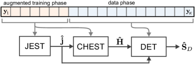
(a) Existing methods separate jammer estimation (JEST) and channel estimation (CHEST) from the jammer-resilient data detection (DET). They are ineffective against jammers that jam the data phase but not the training phase.

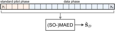
(b) Our method unifies jammer estimation and mitigation, channel estimation, and data detection to deal with jammers regardless of their activity pattern.

Figure 1: The approach to jammer mitigation taken by existing methods (a) compared to the proposed method (b). In the figure, $\mathbf{y}_{1},\dots,\mathbf{y}_{K}$ are the receive signals, and $\hat{}\mathbf{j},\hat{}\mathbf{H}$, and $\hat{}\mathbf{S}_{D}$ are the estimates of the jammer channel, the UE channel matrix, and the UE data symbols, respectively.

I-B Contributions

To mitigate smart jammers in the massive MU-MIMO uplink, we propose a novel approach that does not depend on the jammer being active during any specific period. Leveraging the fact that a jammer cannot change its subspace instantaneously, we utilize a problem formulation which unifies jammer estimation and mitigation, channel estimation, and data detection, instead of dealing with these tasks independently (cf. fig:maed). We support the soundness of the proposed optimization problem by proving that its global minimum is unique and recovers the transmitted data symbols, given that certain conditions are satisfied. By building on techniques for joint channel estimation and data detection [28, 29, 30, 31, 32, 33, 34], we then develop two efficient iterative algorithms for approximately solving the optimization problem. The first algorithm is called MAED (short for MitigAtion, Estimation, and Detection) and solves the problem approximately using forward-backward splitting (FBS) [35]. The second algorithm is called SO-MAED (short for Soft-Output MAED) and extends MAED with a more informative prior on the data symbols to produce soft symbol estimates. SO-MAED relies on deep unfolding to optimize its parameters [34, 36, 37, 38, 39]. We use simulations with different propagation models to demonstrate that MAED and SO-MAED effectively mitigate a wide variety of naïve and smart jamming attacks without requiring any knowledge about the attack type.

I-C Notation

Matrices and column vectors are represented by boldface uppercase and lowercase letters, respectively. For a matrix $\mathbf{A}$, the conjugate is $\mathbf{A}^{\!\ast}$, the transpose is $\mathbf{A}^{\text{T}}$, the conjugate transpose is $\mathbf{A}^{\text{H}}$, the Moore-Penrose pseudoinverse is $\mathbf{A}^{\dagger}$, the entry in the $\ell$th row and $k$th column is $[\mathbf{A}]_{\ell,k}$, the $k$th column is $\mathbf{a}_{k}$, the submatrix consisting of the columns from $n$ through $m$ is $\mathbf{A}_{[n:m]}$, and the Frobenius norm is $\|\mathbf{A}\|_{F}$. The $N\!\times\!N$ identity matrix is $\mathbf{I}_{N}$. For a vector $\mathbf{a}$, the $\ell_{2}$-norm is $\|\mathbf{a}\|_{2}$, the real part is $\Re\{\mathbf{a}\}$, the imaginary part is $\Im\{\mathbf{a}\}$, and the span is $\textit{span}(\mathbf{a})$. For vectors $\mathbf{a},\mathbf{b}$, we define $[\mathbf{a}^{\text{T}};\mathbf{b}^{\text{T}}]\triangleq[\mathbf{a},\mathbf{b}]^{\text{T}}$. Expectation with respect to a random vector $\mathbf{x}$ is denoted by $\operatorname{\mathbb{E}}_{\mathbf{x}}\mathopen{}\left[\cdot\right]$. We define $i^{2}=-1$. The complex $n$-hypersphere of radius $r$ is denoted by $\mathbb{S}_{r}^{n}$, and $[n:m]$ are the integers from $n$ through $m$.

II System Setup

II-A Transmission Model

We consider the uplink of a massive MU-MIMO system in which $U$ single-antenna UEs transmit data to a $B$ antenna BS in the presence of a single-antenna jammer. The channels are assumed to be frequency flat and block-fading with coherence time $K=T+D$. The first $T$ time slots are used to transmit pilot symbols; the remaining $D$ time slots are used to transmit data symbols. The UE transmit matrix is $\mathbf{S}=[\mathbf{S}_{T},\mathbf{S}_{D}]$, where $\mathbf{S}_{T}\in\mathbb{C}^{U\times T}$ and $\mathbf{S}_{D}\in\mathcal{S}^{U\times D}$ contain the pilots and the data symbols, respectively. The data symbols $\mathbf{S}_{D}$ are drawn i.i.d. uniformly from a constellation $\mathcal{S}$, which is normalized to unit average symbol energy. We assume that the jammer does not prevent the UEs and the BS from establishing synchronization, which allows us to use the discrete-time input-output relation

$$\mathbf{Y}=\mathbf{H}\mathbf{S}+\mathbf{j}\mathbf{w}^{\text{T}}+\mathbf{N}.$$ (1)

Here, $\mathbf{Y}\in\mathbb{C}^{B\times K}$ is the BS receive matrix that contains the $B$-dimensional receive vectors over all $K$ time slots, $\mathbf{H}\in\mathbb{C}^{B\times U}$ models the channel between the UEs and the BS, $\mathbf{j}\in\mathbb{C}^{B}$ models the channel between the jammer and the BS, $\mathbf{w}^{\text{T}}=[\mathbf{w}_{T}^{\text{T}},\mathbf{w}_{D}^{\text{T}}]\in\mathbb{C}^{K}$ contains the jammer transmit symbols over all $K$ time slots, and $\mathbf{N}\in\mathbb{C}^{B\times K}$ models thermal noise consisting of independently and identically distributed (i.i.d.) circularly-symmetric complex Gaussian entries with variance $N_{0}$. Unless stated otherwise, we assume that the jammer’s transmit symbols $\mathbf{w}$ are independent of $\mathbf{S}$. No other assumptions about the distribution of $\mathbf{w}$ are made; in particular, we do not assume that these entries are i.i.d.

In what follows, we use plain symbols for the true channels and transmit signals, variables with a tilde for optimization variables, and quantities with a hat for (approximate) solutions to optimization problems, e.g., $\hat{}\mathbf{S}_{D}$ is the estimate of the UE data symbol matrix $\mathbf{S}_{D}$ as determined by solving an optimization problem with respect to $\tilde{}\mathbf{S}_{D}$.

II-B Model Limitations

We now point out—and discuss the relevance of—a number of limitations of our transmission model.
Our model only considers single-antenna UEs, while multi-antenna UEs and point-to-point (p2p) MIMO are excluded. In principle, our method could also be combined with multi-antenna UEs or p2p MIMO, as long as spatial multiplexing is used. This would simply change the transmission model in (1) to $\mathbf{Y}=\mathbf{H}\mathbf{F}\mathbf{S}+\mathbf{j}\mathbf{w}^{\text{T}}+\mathbf{N}$, where $\mathbf{F}$ is a transmit beamforming matrix which is either block-diagonal (in the case of multi-antenna UEs) or dense (in the case of p2p MIMO). Such a model would raise the question of how to choose the transmit beamformer(s) $\mathbf{F}$, and how to obtain the necessary channel state information at the transmitter(s) in the presence jamming. We leave these issues for future work.
Similarly, we only consider single-antenna jammers. However, the ideas that underlie our methods can also be extended to the mitigation of multi-antenna jammers. We consider the mitigation of multi-antenna jammers with methods similar—but not identical—to the ones in this paper in [40].
Another limitation pertains to our use of a block-fading channel model. Real-world channels do not stay constant for a fixed amount of time and then change abruptly. However, our method does not depend on how the channel changes between coherence blocks, but only on the channel staying (approximately) constant for a certain period of time, which is a reasonable assumption in practice. In real-world channels which change continuously even between coherence intervals, channel knowledge from previous coherence intervals could potentially be used to find effective initializers for our algorithms. We defer such investigations to future work.
We also, for the most part, assume independence between the jammer’s transmit symbols $\mathbf{w}$ and the UEs’ transmit signals $\mathbf{S}$, which comprise the pilots $\mathbf{S}_{T}$ and the data symbols $\mathbf{S}_{D}$. This is motivated by the reasonable assumption that the UEs’ transmit data are a priori unknown to anyone except themselves. The jammer’s time-$k$ transmit symbol $w_{k}$ can thus not depend on the time-$k$ UE data vector $\mathbf{s}_{k}$. In principle, the jammer could try to detect the UE data symbols to make $w_{k}$ dependent on $\mathbf{s}_{1},\dots,\mathbf{s}_{k-L}$, for some processing latency $L\geq 1$. However, such “full-duplex” jamming would be extremely difficult to implement [41]. Also, delayed dependencies (such as replaying the signal of some UE with a delay) would have no bearing on the performance of our method, which does not “mix” the receive signals from different time indexes in processing. The assumption that the jammer transmit symbols do not depend on the pilots $\mathbf{S}_{T}$ is thus reasonable as long as randomized pilots are used (cf. sec:theory), but not necessarily when the pilots are deterministic and known to the jammer (cf. sec:results:eclipsed).
The final limitation is our assumption of perfect synchronization between the UEs and the BS. This is not an innocent assumption, as jammers can inhibit synchronization [26]. However, we consider the question of how to synchronize in the presence of jamming as a separate research problem that is outside the scope of this paper and for which we refer to [27].

​​ ​​​ ​​

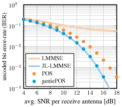
(a) mitigation of a barrage jammer

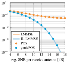
(b) failed mitigation of a smart jammer

Figure 2: An example that illustrates how methods that estimate the jammer’s channel based on a subset of samples fail when facing a smart jammer.

III Motivating Example

To understand the challenge posed by smart jammers as opposed to barrage jammers, we start by considering the motivating example of fig:example, which shows uncoded bit error-rates (BERs) of different receivers (LMMSE, JL-LMMSE, geniePOS, POS) for an i.i.d. Rayleigh fading MU-MIMO system with $B=128$ BS antennas and $U=32$ UEs that transmit 16-QAM symbols under a jamming attack. In fig:example:success the system is attacked by a barrage jammer that transmits i.i.d. Gaussian symbols and whose receive power exceeds that of the average UE by 30 dB. The different receivers operate as follows:

III-1 LMMSE

This receiver estimates the channel matrix using orthogonal pilots with a least squares (LS) estimator followed by a linear minimum mean square error (LMMSE) detector.

III-2 JL-LMMSE

This receiver works identical to the LMMSE receiver but operates in a jammerless (“JL”) system.

III-3 geniePOS

This receiver serves as a baseline and is furnished with ground-truth knowledge of the jammer channel $\mathbf{j}$. It nulls the jammer by orthogonally projecting the receive signals on the orthogonal complement (“POS” is short for Projection onto the Orthogonal Subspace) of $\textit{span}(\mathbf{j})$ using the matrix $\mathbf{P}_{\mathbf{j}}=\mathbf{I}_{B}-\mathbf{j}\mathbf{j}^{\dagger}$[42, Sec. 2.6.1], where $\mathbf{j}^{\dagger}=\mathbf{j}^{\text{H}}/\|\mathbf{j}\|_{2}^{2}$, as

$$\mathbf{P}_{\mathbf{j}}\mathbf{Y} =\mathbf{P}_{\mathbf{j}}\,\mathbf{H}\mathbf{S}+\mathbf{P}_{\mathbf{j}}\,\mathbf{j}\mathbf{w}^{\text{T}}+\mathbf{P}_{\mathbf{j}}\,\mathbf{N}$$ (2)

$$=\mathbf{P}_{\mathbf{j}}\,\mathbf{H}\mathbf{S}+\mathbf{P}_{\mathbf{j}}\,\mathbf{N},$$ (3)

since $\mathbf{P}_{\mathbf{j}}\,\mathbf{j}=\mathbf{0}$. The result is an effective jammerless system with receive signal $\mathbf{Y}_{\mathbf{P}}=\mathbf{P}_{\mathbf{j}}\mathbf{Y}$, effective channel matrix $\mathbf{H}_{\mathbf{P}}=\mathbf{P}_{\mathbf{j}}\mathbf{H}$, and (colored) noise $\mathbf{N}_{\mathbf{P}}=\mathbf{P}_{\mathbf{j}}\mathbf{N}\sim\mathcal{C}\mathcal{N}(\mathbf{0},N_{0}\mathbf{P}_{\mathbf{j}})$. Finally, geniePOS performs LS channel estimation and subsequent LMMSE data detection in this projected system [6].

III-4 POS

This receiver works analogously to geniePOS, except that it is not furnished with ground-truth knowledge of the jammer channel—instead, this receiver estimates the jammer subspace $\mathbf{j}/\|\mathbf{j}\|_{2}$ based on ten receive samples in which the UEs do not transmit and only the jammer is active. If the matrix received in that period is denoted by $\mathbf{Y}_{\text{J}}$, then the jammer subspace is estimated as the left-singular vector of the largest singular value of $\mathbf{Y}_{\text{J}}$.

fig:example:success shows that geniePOS effectively mitigates the jammer, achieving a performance virtually identical to that of the jammer-free JL-LMMSE receiver. Indeed, geniePOS nulls the jammer perfectly, so that the only performance loss comes from the loss of one degree-of-freedom in the receive signal. POS is not as effective, since it nulls the jammer only imperfectly due to its noisy estimate of the jammer subspace. However, this method still mitigates the jammer with a loss of less than 2 dB in SNR (at $0.1\%$ BER) compared to the jammer-free JL-LMMSE receiver.

Remark 1.

Reserving time slots for jammer estimation in which the UEs cannot transmit reduces the achievable data rates.

Contrastingly, in fig:example:fail the attacking (smart) jammer is aware of the POS receiver’s mitigation scheme and suspends transmission during the time slots that are used to estimate its subspace. The POS receiver’s subspace estimate is thus based entirely on noise and is completely independent of the jammer’s true channel $\mathbf{j}$. Consequently, the mitigation mechanism fails spectacularly, yielding a bit error-rate identical to the non-mitigating LMMSE receiver.

IV Joint Jammer Estimation and Mitigation, Channel Estimation, and Data Detection

The foregoing example has demonstrated the danger of estimating the jammer’s subspace (or other characteristics of the jammer, such as its spatial covariance) based on a certain subset of receive samples when facing a smart jammer. We therefore propose a method that does not depend on the jammer being active during any specific period. This independence is achieved by considering the receive signal over an entire coherence interval at once and exploiting the fact that the jammer subspace stays fixed within that period, regardless of the jammer’s activity pattern or transmit sequence. Specifically, we first propose a novel optimization problem that combines a tripartite goal of (i) mitigating the jammer’s interference by locating its subspace $\textit{span}(\mathbf{j})$ and projecting the receive matrix $\mathbf{Y}$ onto the orthogonal complement of that subspace, (ii) estimating the channel matrix $\mathbf{H}$, and (iii) recovering the data matrix $\mathbf{S}_{D}$. We then establish the soundness of the proposed optimization problem by proving that, under certain sensible conditions, and assuming negligible thermal noise, the minimum is unique and corresponds to the desired solution; in particular, solving the problem recovers the data matrix $\mathbf{S}_{D}$. Finally, we develop efficient iterative algorithms that approximately solve the proposed optimization problem.

IV-A The Optimization Problem

To motivate our optimization problem, we will make the simplifying assumption that the thermal noise is so low as to be negligible: $\mathbf{N}\approx\mathbf{0}$. The reason for making the low-noise assumption is not that it is ultimately necessary for our method to work (indeed, our numerical results in sec:results show our method to work well also when the noise is not negligible), but since the absence of noise helps to understand the problem, and since any sensible jammer mitigation method should also work in the absence of additional thermal noise.

We start our derivation by considering the maximum-likelihood (ML) problem for joint channel estimation and data detection (JED), assuming—in a first step—no jamming activity (i.e., assuming $\mathbf{w}=\mathbf{0}$). In that case, the ML JED problem is [28]

$$\big{\{}\hat{}\mathbf{H},\hat{}\mathbf{S}_{D}\big{\}} =\operatorname*{arg\;min}_{\begin{subarray}{c}\hskip 3.69885pt\tilde{}\mathbf{H}\in\mathbb{C}^{B\times U}\\ \tilde{}\mathbf{S}_{D}\in\mathcal{S}^{U\times D}\end{subarray}}\!\big{\|}\mathbf{Y}-\tilde{}\mathbf{H}\tilde{}\mathbf{S}\big{\|}^{2}_{F},$$ (4)

where we define $\tilde{}\mathbf{S}\triangleq[\mathbf{S}_{T},\tilde{}\mathbf{S}_{D}]$ for brevity and leave the dependence on $\tilde{}\mathbf{S}_{D}$ implicit. This objective already integrates the goals of estimating the channel matrix and detecting the data symbols: If the noise $\mathbf{N}$ is small enough to be negligible, the problem is minimized by the true channel and data matrices,

$$\|\mathbf{Y}-\mathbf{H}\mathbf{S}\|^{2}_{F}{\color[rgb]{0,0,0}=\|\mathbf{N}\|_{F}^{2}}\approx 0,$$ (5)

where the pilot matrix $\mathbf{S}_{T}$ ensures uniqueness. Let us now consider how (5) is affected by the presence of significant jamming activity: $\|\mathbf{w}\|_{2}^{2}\gg 0$. In that case, the jammer will cause a residual

$$\|\mathbf{Y}-\mathbf{H}\mathbf{S}\|^{2}_{F} =\|\mathbf{j}\mathbf{w}^{\text{T}}+\mathbf{N}\|^{2}_{F}$$ (6)

$$\approx\|\mathbf{j}\mathbf{w}^{\text{T}}\|^{2}_{F}\gg 0$$ (7)

​​​ when plugging the true channel and data matrices into eq:ml_jed. The step in (7) follows because we assumed $\|\mathbf{w}\|_{2}^{2}\gg 0$ and $\mathbf{N}\approx\mathbf{0}$. Considering (7), there might now be a tuple $\{\tilde{}\mathbf{H},\tilde{}\mathbf{S}_{D}\}$ with $\tilde{}\mathbf{S}_{D}\neq\mathbf{S}_{D}$ such that $\|\mathbf{Y}-\tilde{}\mathbf{H}\tilde{}\mathbf{S}\|^{2}_{F}<\|\mathbf{Y}-\mathbf{H}\mathbf{S}\|^{2}_{F}$.

Note, however, that the residual $\mathbf{j}\mathbf{w}^{\text{T}}$ in (7) is a rank-one matrix whose columns are all contained in $\textit{span}(\mathbf{j})$, regardless of the jamming signal $\mathbf{w}$. Consider therefore what happens when we take the matrix

$$\tilde{}\mathbf{P}\triangleq{\color[rgb]{0,0,0}\mathbf{I}-\tilde{}\mathbf{p}\tilde{}\mathbf{p}^{\dagger}=~{}}\mathbf{I}-\tilde{}\mathbf{p}\tilde{}\mathbf{p}^{\text{H}},~{}\tilde{}\mathbf{p}\in\mathbb{S}_{1}^{B},$$ (8)

which projects a signal onto the orthogonal complement of some arbitrary one-dimensional subspace $\textit{span}(\tilde{}\mathbf{p})$[42, Sec. 2.6.1], and then apply that projection to the objective of (4):

$$\|\tilde{}\mathbf{P}(\mathbf{Y}-\tilde{}\mathbf{H}\tilde{}\mathbf{S})\|^{2}_{F}.$$ (9)

If we now plug the true channel and data matrices into eq:ml_p_jed (still assuming negligibility of the noise $\mathbf{N}$), then we obtain

$$\|\tilde{}\mathbf{P}(\mathbf{Y}-\mathbf{H}\mathbf{S})\|^{2}_{F} =\|\tilde{}\mathbf{P}\mathbf{j}\mathbf{w}^{\text{T}}+\tilde{}\mathbf{P}\mathbf{N}\|^{2}_{F}$$ (10)

$$\approx\|\tilde{}\mathbf{P}\mathbf{j}\mathbf{w}^{\text{T}}\|^{2}_{F}\geq 0,$$ (11)

with equality if and only if $\tilde{}\mathbf{p}$ is collinear with $\mathbf{j}$. In other words, the unit vector $\tilde{}\mathbf{p}$ which in combination with the true channel and data matrices minimizes (9) is collinear with the jammer’s channel. In this case, $\tilde{}\mathbf{P}=\mathbf{I}_{B}-(\mathbf{j}/\|\mathbf{j}\|_{2})(\mathbf{j}^{\text{H}}/\|\mathbf{j}\|_{2})=\mathbf{I}_{B}-\mathbf{j}\mathbf{j}^{\dagger}$ coincides with the matrix $\mathbf{P}_{\mathbf{j}}$ from (2) which projects onto the orthogonal complement of the jammer’s subspace.

Thus, if the noise $\mathbf{N}$ is negligible, and if (i) $\tilde{}\mathbf{P}$ is the projection onto the orthogonal complement of $\textit{span}(\mathbf{j})$, (ii) $\tilde{}\mathbf{H}$ is the true channel matrix, and (iii) $\tilde{}\mathbf{S}$ contains the true data matrix, then the tuple $\{\tilde{}\mathbf{p},\tilde{}\mathbf{H},\tilde{}\mathbf{S}\}$ minimizes (9). These are, of course, exactly the goals which we want to attain. We thus formulate our joint jammer estimation and mitigation, channel estimation, and data detection problem as follows:

$$\big{\{}\hat{}\mathbf{p},\hat{}\mathbf{H}_{\mathbf{P}},\hat{}\mathbf{S}_{D}\big{\}} =\operatorname*{arg\;min}_{\begin{subarray}{c}\tilde{}\mathbf{p}\in\mathbb{S}_{1}^{B}\hskip 3.98337pt\\ \hskip 3.69885pt\tilde{}\mathbf{H}_{\mathbf{P}}\in\mathbb{C}^{B\times U}\\ \tilde{}\mathbf{S}_{D}\in\mathcal{S}^{U\times D}\end{subarray}}\!\big{\|}\tilde{}\mathbf{P}\mathbf{Y}-\tilde{}\mathbf{H}_{\mathbf{P}}\tilde{}\mathbf{S}\big{\|}^{2}_{F}.\!$$ (12)

Note that, compared to (9), we have absorbed the projection matrix $\tilde{}\mathbf{P}$ directly into the unknown channel matrix $\tilde{}\mathbf{H}_{\mathbf{P}}$, which replaces the product $\tilde{}\mathbf{P}\tilde{}\mathbf{H}$ in (9). Otherwise, the columns of $\tilde{}\mathbf{H}$ would not be fully determined, since—because of the projection $\tilde{}\mathbf{P}$—the magnitude of their components in the direction of $\tilde{}\mathbf{p}\approx\mathbf{j}$ would be undetermined: The objective in (9) would be unable to distinguish between two different channel estimates $\tilde{}\mathbf{H}$ and $\tilde{}\mathbf{H}^{\prime}$ when $\tilde{}\mathbf{H}-\tilde{}\mathbf{H}^{\prime}=\mathbf{j}\tilde{}\mathbf{w}^{\text{T}}$ for some $\tilde{}\mathbf{w}\in\mathbb{C}^{U}$.

IV-B Theory

We have derived the optimization problem (12) based on intuitive but non-rigorous arguments. Thus, we will now support the soundness of (12) by proving that, under certain sensible conditions, and assuming that the noise is negligible, its solution is unique and guaranteed to recover the true data matrix. The assumption of negligible noise can be understood as a limiting case of a high SNR scenario.

We make the following assumptions: The channel matrix $\mathbf{H}$ has full column rank $U$, the jammer channel $\mathbf{j}$ is not included in the column space of $\mathbf{H}$, and the pilot matrix $\mathbf{S}_{T}$ has full row rank $U$. In addition, we define a concept which may seem cryptic at first, but which will be clarified later.

Definition 1.

The jammer is eclipsed in a given coherence interval if there exists a matrix $\tilde{\mathbf{S}}_{D}\in\mathcal{S}^{U\times D}$, $\tilde{\mathbf{S}}_{D}\neq\mathbf{S}_{D}$, such that the matrix $\bm{\Sigma}\!\triangleq\![\mathbf{S}_{D}-\tilde{\mathbf{S}}_{D};\mathbf{w}_{D}^{\text{T}}-\mathbf{w}_{T}^{\text{T}}\mathbf{S}_{T}^{\dagger}\tilde{\mathbf{S}}_{D}]$ has rank one.

We can now state our result; the proof is in app:proof1.

Theorem 1.

In the absence of noise, $\mathbf{N}=\mathbf{0}$, and if the jammer is not eclipsed, then the problem in (12) has the unique solution $\{\hat{}\mathbf{p},\hat{}\mathbf{H}_{\mathbf{P}},\hat{}\mathbf{S}_{D}\}=\{\mathbf{p},\mathbf{P}\mathbf{H},\mathbf{S}_{D}\}$ (In fact, $\hat{\mathbf{p}}$ is unique only up to an immaterial phase shift, $\hat{\mathbf{p}}=\alpha\mathbf{p},|\alpha|=1$.)

In other words, as long as the jammer is not ecplised, the problem in (12) is uniquely minimized by the true jammer subspace, projected channel matrix, and data matrix. We now shed light on the notion of eclipsedness. We will also show in thm:maed2 that—if randomized pilots are used—the jammer is typically not eclipsed in almost all cases. In fact, the jammer is typically not eclipsed even when deterministic pilots are used.

Eclipsing describes the existence of a certain relationship between the signal and the jamming subspace that creates an ambiguity when trying to resolve between the two. In essence, the jammer is eclipsed if its jamming signal $\mathbf{w}$ is such that multiple possible “explanations” of the receive signal $\mathbf{Y}$ exist which are consistent with the pilot matrix $\mathbf{S}_{T}$ and under some of which the jammer is not recognized as the jammer; cf. the discussion of (52) in app:proof1. This is best explained by considering two emblematic cases of an eclipsed jammer:

IV-B1 An inactive jammer (or no jammer)

Clearly, if $\mathbf{w}=\mathbf{0}$, then the last row of $\bm{\Sigma}$ is zero for all $\tilde{\mathbf{S}}_{D}$, including those that differ from $\mathbf{S}_{D}$ only in a single row or column, so that eclipsing occurs. In this case, there is a mismatch between the jammerless actual wireless transmission and the jammed model in (1). Since there is no jammer subspace to identify, the choice of the projection $\tilde{}\mathbf{P}$ is undetermined, so that thm:maed no longer applies. Interestingly, this degenerate case implies that our jammer mitigation method may in fact require the presence of jamming to operate at full effectiveness. In this regard, see also the jammerless experiment in sec:results:eclipsed.

IV-B2 The jammer transmits a valid pilot sequence

If the jammer knows the pilots $\mathbf{S}_{T}$ and transmits the $k$th UE’s pilot sequence in the training phase and constellation symbols in the data phase, then there are no formal grounds for the receiver to distinguish between the jammer and the $k$th UE. It can readily be shown that, besides the desired solution $\{\hat{}\mathbf{p},\hat{}\mathbf{H}_{\mathbf{P}},\hat{}\mathbf{S}_{D}\}=\{\mathbf{p},\mathbf{P}\mathbf{H},\mathbf{S}_{D}\}$, there exists then another solution to (12) which identifies the $k$th UE as the jammer, nulls that UE by setting $\hat{}\mathbf{p}=\mathbf{h}_{k}/\|\mathbf{h}_{k}\|$, and instead identifies the jammer as the $k$th UE by estimating

$$\hat{}\mathbf{H}_{\mathbf{P}} =\hat{}\mathbf{P}[\mathbf{h}_{1},\dots,\mathbf{h}_{k-1},\mathbf{j},\mathbf{h}_{k+1},\dots,\mathbf{h}_{U}],$$ (13)

$$\hat{}\mathbf{S}_{D} =[\mathbf{s}_{D,1}^{\text{T}},\dots,\mathbf{s}_{D,k-1}^{\text{T}},\mathbf{w}_{D}^{\text{T}},\mathbf{s}_{D,k+1}^{\text{T}},\dots,\mathbf{s}_{D,U}^{\text{T}}]^{\text{T}},$$ (14)

where $\mathbf{s}_{D,u}$ is the $u$th row of $\mathbf{S}_{D}$. This is a case of eclisping, since for $\hat{}\mathbf{S}_{D}=\tilde{}\mathbf{S}_{D}$, all rows of $\bm{\Sigma}$ except the $u$th row are zero, so that $\bm{\Sigma}$ has rank one.

Besides these two paradigmatic cases, eclipsing may also happen “accidentally” in cases where, for some $\tilde{}\mathbf{S}_{D}$, the symbol error matrix $\mathbf{S}_{D}-\tilde{}\mathbf{S}_{D}$ has rank one and its rows are, by coincidence, all collinear with $\mathbf{w}_{D}^{\text{T}}-\mathbf{w}_{T}^{\text{T}}\mathbf{S}_{T}^{\dagger}\tilde{\mathbf{S}}_{D}$.

However, we will now show that if the jammer does not know the pilot sequences, e.g., because they are drawn at random by the BS and secretly communicated to the UEs, then an active jammer (where $\mathbf{w}\neq\mathbf{0}$) is typically not eclipsed. Thus, to obtain the best possible resilience against smart jammers, randomized pilots should be used. To show this, we consider a case in which the pilot matrix $\mathbf{S}_{T}$ is square; the proof is relegated to app:proof2.

Theorem 2.

If the pilot matrix $\mathbf{S}_{T}$ is drawn uniformly over the set of $U\times U$ unitary matrices and if $\mathbf{w}_{T}\neq\mathbf{0}$ and $\mathbf{w}_{D}\neq\mathbf{0}$ are independent of $\mathbf{S}_{T}$, then the probability that the jammer eclipses is bounded from above by $|\mathcal{S}|^{3U}|\mathcal{S}|^{-(U-3)D}$, i.e., the probability of eclipsing decreases exponentially in the number $D$ of data time slots processed simultaneously.

Example 1.

If the assumptions of thm:maed2 are satisfied, and if $\mathcal{S}$ is $16$-QAM, $U=32$ and $D=128$, as in most of our experiments in sec:results, then the probability of eclipsing is at most $16^{-3616}\approx 10^{-4338}$. Even if $\mathcal{S}$ is QPSK, $U=4$, and one processes only $D=20$ data slots simultaneously, the probability of eclipsing is bounded by $1.6\times 10^{-5}$.

Remark 2.

It is by no means necessary to use random pilots to avoid eclipsing. Nor is it necessary that both $\mathbf{w}_{T}$ and $\mathbf{w}_{D}$ are distinct from zero. Another sufficient condition for the jammer to be eclipsed only with zero probability is, e.g., if $\mathbf{w}$ has at least two independent marginals with continuous distribution. The main point is that, unless the jammer choses its input sequence as some (partially randomized) function of the pilot matrix $\mathbf{S}_{T}$, eclipsing is the rare exception, not the norm. In this regard, see also the simulation results in sec:results.

Remark 3.

The fact that reliable communication in the presence of jamming can be assured if the BS and UEs share a common secret that enables them to use a randomized communication scheme, but not otherwise, is reminiscent of information-theoretic results which prove a similar dichotomy on a more fundamental level. See [43, Sec. V] and references therein.

V Forward-Backward Splitting with a Box Prior

We now provide the first of two algorithms for approximately solving the joint jammer estimation and mitigation, channel estimation, and data detection problem in (12). Note first of all that the objective is quadratic in $\tilde{}\mathbf{H}_{\mathbf{P}}$, so we can derive the optimal value of $\tilde{}\mathbf{H}_{\mathbf{P}}$ as a function of $\tilde{}\mathbf{P}$ and $\tilde{}\mathbf{S}$ as

$$\hat{}\mathbf{H}_{\mathbf{P}}=\tilde{}\mathbf{P}\mathbf{Y}\tilde{}\mathbf{S}^{\dagger},$$ (15)

where $\tilde{}\mathbf{S}^{\dagger}=\tilde{}\mathbf{S}^{\text{H}}(\tilde{}\mathbf{S}\tilde{}\mathbf{S}^{\text{H}})^{-1}$. Substituting $\hat{}\mathbf{H}_{\mathbf{P}}$ back into (12) yields an optimization problem which only depends on $\tilde{}\mathbf{p}$ and $\tilde{}\mathbf{S}_{D}$:

$$\big{\{}\hat{}\mathbf{p},\hat{}\mathbf{S}_{D}\big{\}}=\operatorname*{arg\;min}_{\begin{subarray}{c}\tilde{}\mathbf{p}\in\mathbb{S}_{1}^{B}\hskip 3.98337pt\\ \tilde{}\mathbf{S}_{D}\in\mathcal{S}^{D\times U}\end{subarray}}\big{\|}\tilde{}\mathbf{P}\mathbf{Y}(\mathbf{I}_{K}-\tilde{}\mathbf{S}^{\dagger}\tilde{}\mathbf{S})\big{\|}^{2}_{F}.$$ (16)

Solving (16) remains difficult due to its combinatorial nature, so we resort to solving it approximately. First, we relax the constraint set $\mathcal{S}$ to its convex hull $\mathcal{C}\triangleq\textit{conv}(\mathcal{S})$ as in [31]. This can be viewed as replacing the probability mass function over the constellation $\mathcal{S}$, which represents the true symbol prior, with a box prior that is uniform over $\mathcal{C}$ and zero elsewhere [44]. We then approximately solve this relaxed problem formulation in an iterative fashion by alternating between a forward-backward splitting descent step in $\tilde{}\mathbf{S}$ and a minimization step in $\tilde{}\mathbf{P}$.

V-A Forward-Backward Splitting Step in $\tilde{}\mathbf{S}$

Forward-backward splitting (FBS) [35], also called proximal gradient descent[45], is an iterative method for solving convex optimization problems of the form

$$\operatorname*{arg\;min}_{\tilde{}\mathbf{s}}\,f(\tilde{}\mathbf{s})+g(\tilde{}\mathbf{s}),$$ (17)

where $f$ is convex and differentiable, and $g$ is convex but not necessarily differentiable, smooth, or bounded. Starting from an initialization vector $\tilde{}\mathbf{s}^{(0)}$, FBS solves the problem in (17) iteratively by computing

$$\tilde{}\mathbf{s}^{(t+1)}=\text{prox}_{g}\big{(}\tilde{}\mathbf{s}^{(t)}-\tau^{(t)}\nabla f(\tilde{}\mathbf{s}^{(t)});\tau^{(t)}\big{)}.$$ (18)

Here, $\tau^{(t)}$ is the stepsize at iteration $t$, $\nabla f(\tilde{}\mathbf{s})$ is the gradient of $f(\tilde{}\mathbf{s})$, and $\text{prox}_{g}$ is the proximal operator of $g$, defined as [45]

$$\text{prox}_{g}(\mathbf{x};\tau)=\operatorname*{arg\;min}_{\tilde{}\mathbf{x}}\tau g(\tilde{}\mathbf{x})+\frac{1}{2}\|\mathbf{x}-\tilde{}\mathbf{x}\|_{2}^{2}.$$ (19)

For a suitable sequence of stepsizes $\{\tau^{(t)}\}$, FBS solves convex optimization problems exactly. FBS can also be used to approximately solve non-convex problems, although there are typically no guarantees for optimality or even convergence [35]. For the optimization problem in eq:obj3, we define $f$ and $g$ as

$$f(\tilde{}\mathbf{S}) =\big{\|}\tilde{}\mathbf{P}\mathbf{Y}(\mathbf{I}_{K}-\tilde{}\mathbf{S}^{\dagger}\tilde{}\mathbf{S})\big{\|}^{2}_{F}$$ (20)

and

$$g(\tilde{}\mathbf{S}) =\begin{cases}0&\text{if }\,\tilde{}\mathbf{S}_{[1:T]}=\mathbf{S}_{T}\text{ and }\tilde{}\mathbf{S}_{[T+1:K]}\in\mathcal{C}^{U\times D}\!\!\!\\ \infty&\text{else}.\end{cases}$$ (21)

The gradient of $f$ in $\tilde{}\mathbf{S}$ is given by

$$\nabla f(\tilde{}\mathbf{S})=-(\mathbf{Y}\tilde{}\mathbf{S}^{\dagger})^{\text{H}}\tilde{}\mathbf{P}\mathbf{Y}(\mathbf{I}_{K}-\tilde{}\mathbf{S}^{\dagger}\tilde{}\mathbf{S}),$$ (22)

and the proximal operator for $g$ is simply the orthogonal projection onto $\mathcal{C}$, which acts entrywise on $\tilde{}\mathbf{S}$ as

$$[\text{prox}_{g}(\tilde{}\mathbf{S};\tau)]_{u,k}=\begin{cases}[\mathbf{S}_{T}]_{u,k}&\text{ if }k\in[1:T]\\ \text{proj}_{\mathcal{C}}([\tilde{}\mathbf{S}]_{u,k})&\text{ else,}\end{cases}$$ (23)

where the function $\text{proj}_{\mathcal{C}}$ is given as

$$\text{proj}_{\mathcal{C}}(x)=\, \min\{\max\{\Re(x),-\lambda\},\lambda\}$$

$$+i\min\{\max\{\Im(x),-\lambda\},\lambda\},$$ (24)

where $\lambda$ denotes the edge of the constellation’s convex hull $\mathcal{C}$, see fig:constellations. The value of $\lambda$ is determined by the fact that the transmit constellations are scaled to unit average symbol energy (cf. sec:setup). Specifically, we have $\lambda=\sqrt{\nicefrac{{1}}{{2}}}$ for a QPSK constellation and $\lambda=\sqrt{\nicefrac{{9}}{{10}}}$ for a 16-QAM constellation. To select the per-iteration stepsizes $\{\tau^{(t)}\}$, we use the Barzilai-Borwein method [46].

V-B Minimization Step in $\tilde{}\mathbf{P}$

After each FBS step in $\tilde{}\mathbf{S}$, we minimize (16) with respect to the vector $\tilde{}\mathbf{p}$. Defining the residual matrix $\tilde{}\mathbf{E}\triangleq\mathbf{Y}(\mathbf{I}_{K}-\tilde{\mathbf{S}}^{\dagger}\tilde{\mathbf{S}})$ and performing standard algebraic manipulations yields

$$\hat{}\mathbf{p} =\operatorname*{arg\;min}_{\tilde{}\mathbf{p}\in\mathbb{S}_{1}^{B}}\big{\|}\tilde{}\mathbf{P}\tilde{}\mathbf{E}\big{\|}^{2}_{F}$$ (25)

$$=\operatorname*{arg\;max}_{\tilde{}\mathbf{p}\in\mathbb{S}_{1}^{B}}\,\tilde{}\mathbf{p}^{\text{H}}\tilde{}\mathbf{E}\tilde{}\mathbf{E}^{\text{H}}\tilde{}\mathbf{p}.$$ (26)

It follows that the vector $\hat{}\mathbf{p}$ minimizing (16) for a fixed $\tilde{}\mathbf{S}$ is the unit vector that maximizes the Rayleigh quotient of $\tilde{}\mathbf{E}\tilde{}\mathbf{E}^{\text{H}}$. The solution is the unit-$2$-norm eigenvector $\mathbf{v}_{1}(\tilde{}\mathbf{E}\tilde{}\mathbf{E}^{\text{H}})$ associated with the largest eigenvalue of $\tilde{}\mathbf{E}\tilde{}\mathbf{E}^{\text{H}}$,

$$\hat{}\mathbf{p}=\mathbf{v}_{1}(\tilde{}\mathbf{E}\tilde{}\mathbf{E}^{\text{H}}).$$ (27)

Calculating this eigenvector in every iteration of our algorithm would be computationally expensive, so we approximate it using a single power iteration [42, Sec. 8.2.1], i.e., we estimate

$$\hat{}\mathbf{p}^{(t+1)}=\frac{\tilde{}\mathbf{E}^{(t+1)}(\tilde{}\mathbf{E}^{(t+1)})^{\text{H}}\hat{}\mathbf{p}^{(t)}}{\|\tilde{}\mathbf{E}^{(t+1)}(\tilde{}\mathbf{E}^{(t+1)})^{\text{H}}\hat{}\mathbf{p}^{(t)}\|_{2}},$$ (28)

where the power method is initialized with the subspace estimate $\hat{}\mathbf{p}^{(t)}$ from the previous algorithm iteration.

V-C Preprocessing

If the algorithm starts directly with a gradient descent step in the direction of (22), one runs the risk of advancing significantly into the wrong direction—especially if the jammer is extremely strong, since a strong jammer will also lead to a large gradient amplitude. Empirically, we observe that such a large initial digression can be problematic (if, e.g., the jammer is $\geq\!50$ dB stronger than the average UE). It might therefore be tempting to start the algorithm directly with a projection step: If one initializes $\tilde{}\mathbf{S}^{(0)}=\mathbf{0}_{U\times D}$, then $\tilde{}\mathbf{E}^{(0)}=\mathbf{Y}$, so that the algorithm starts by nulling the dimension of $\mathbf{Y}$ which contains the most energy. In the presence of a strong jammer, this is a sensible strategy since this dimension then corresponds to the jammer subspace. However, if the received jamming energy is small compared to the energy received from the UEs (e.g., because the jammer does not transmit at all during a given coherence interval), then such a projection would inadvertently null the strongest user. To thread the needle between these two cases—largely removing a strong jammer before the first gradient step, but not removing any legitimate UEs when a strong jammer is absent—we propose to start with a regularized projection step: The algorithm starts by a projection onto the orthogonal complement of the eigenvector of the largest eigenvalue of

$$\mathbf{Y}\mathbf{Y}^{\text{H}}+\mathbf{\Gamma},$$ (29)

where $\mathbf{\Gamma}\in\mathbb{C}^{B\times B}$ is a constant regularization matrix. The basic idea is that this regularization matrix is still overshadowed by very strong jammers, so that these are largely nulled within the preprocessing, while, in the presence of only a weak jammer (or no jammer), the regularization matrix has a sufficiently diverting impact on the eigenvectors to prevent the nulling of a legitimate UE. There are countless ways of choosing such a regularization matrix. (Note, however, that $\mathbf{\Gamma}$ should not be a multiple of the identity matrix $\mathbf{I}_{B}$, which does not affect the eigenvectors of (29).) For simplicity, we set $\mathbf{\Gamma}$ to the all-zero matrix, except for the top left entry, which is set to $0.1BUK$.

V-D Algorithm Complexity

We now have all the ingredients for MAED, which is summarized in alg:maed. Its only input is the receive matrix $\mathbf{Y}$, as it does not even require an estimate of the thermal noise variance $N_{0}$. MAED is initialized with $\tilde{}\mathbf{S}^{(0)}=[\mathbf{S}_{T},\mathbf{0}_{U\times D}]$ and $\tau^{(0)}=\tau=0.1$, and runs for a fixed number of $t_{\max}$ iterations.

The complexity of MAED is dominated by the eigenvector calculation in the preprocessing step (which could be reduced by using the power method approximation) as well as the gradient computation in line 5 of alg:maed, which has a complexity of $O(3BUK+2U^{2}K+U^{3})$. The overall complexity of MAED is therefore $O(t_{\max}(3BUK+2U^{2}K+U^{3}))$. Note, however, that MAED detects $D$ data vectors at once. Thus, the computational complexity per detected symbol is only $O(t_{\max}(3BK+2KU+U^{2})/D)$.

VI Soft-Output Estimates with Deep Unfolding

MAED, which corresponds to the algorithm proposed in [1] (adding the new preprocessing step), already attains the goal of mitigating smart jammers, see sec:results. However, its detection performance can be suboptimal, especially when higher-order transmit constellations such as 16-QAM are used. The culprit is the box prior of MAED, which does not fully exploit the discrete nature of the transmit constellation. In particular, the box prior is uninformative about the constellation symbols in the interior of $\mathcal{C}$. To improve detection performance, we now provide a second algorithm for approximately solving the problem in (12). This second algorithm builds on MAED but replaces the proximal operator in (23), which enforces MAED’s box prior, by an approximate posterior mean estimator (PME) based on the discrete symbol prior as in [34]. Since the PME also enables meaningful soft-output estimates of the bits that underlie the transmitted data symbols, we refer to this second algorithm as soft-output MAED (SO-MAED).

Algorithm 1 MAED

1:input: $\mathbf{Y}$

2:initialize $\tilde{}\mathbf{S}^{(0)}\!=\!\left[\mathbf{S}_{T},\mathbf{0}_{U\!\times\!D}\right]\!,\tilde{}\mathbf{p}^{(0)}\!=\!\mathbf{v}_{1}(\mathbf{Y}\mathbf{Y}^{\text{H}}\!+\mathbf{\Gamma}),\tau^{(0)}\!=\tau$

3:$\tilde{}\mathbf{P}^{(0)}=\mathbf{I}_{B}-\tilde{}\mathbf{p}^{(0)}\tilde{}\mathbf{p}^{(0)}{}^{\text{H}}$

4:for $t=0$ to $t_{\max}-1$ do

5:   $\nabla f(\tilde{}\mathbf{S}^{(t)})=-\big{(}\mathbf{Y}\tilde{}\mathbf{S}^{(t)}{}^{\dagger}\big{)}^{\text{H}}\tilde{}\mathbf{P}^{(t)}\mathbf{Y}(\mathbf{I}_{K}-\tilde{}\mathbf{S}^{(t)}{}^{\dagger}\tilde{}\mathbf{S}^{(t)})$

6:   $\tilde{}\mathbf{S}^{(t+1)}=\text{prox}_{g}\big{(}\tilde{}\mathbf{S}^{(t)}-\tau^{(t)}\nabla f(\tilde{}\mathbf{S}^{(t)})\big{)}$

7:   $\tilde{}\mathbf{E}^{(t+1)}=\mathbf{Y}(\mathbf{I}_{K}-\tilde{}\mathbf{S}^{(t+1)}{}^{\dagger}\tilde{}\mathbf{S}^{(t+1)})$

8:   $\tilde{}\mathbf{p}^{(t+1)}=\tilde{}\mathbf{E}^{(t+1)}\tilde{\mathbf{E}}^{(t+1)}{}^{\text{H}}\,\tilde{}\mathbf{p}^{(t)}/\|\tilde{}\mathbf{E}^{(t+1)}\tilde{\mathbf{E}}^{(t+1)}{}^{\text{H}}\,\tilde{}\mathbf{p}^{(t)}\|_{2}$

9:   $\tilde{}\mathbf{P}^{(t+1)}=\mathbf{I}_{B}-\tilde{}\mathbf{p}^{(t+1)}\tilde{}\mathbf{p}^{(t+1)}{}^{\text{H}}$

10:   compute $\tau^{(t+1)}$ by following [35, Sec. 4.1]

11:end for

12:output: $\tilde{}\mathbf{S}^{(t_{\max})}_{[T+1:K]}$

VI-A Approximate Posterior-Mean Estimation

To replace the proximal operator following the gradient descent step in (18) with a more appropriate data symbol estimator which takes into account the discrete constellation $\mathcal{S}$, we model the per-iteration outputs of the gradient descent step

$$\tilde{}\mathbf{X}^{(t)}=\tilde{}\mathbf{S}^{(t)}-\tau^{(t)}\nabla f(\tilde{}\mathbf{S}^{(t)})$$ (30)

as

$$\tilde{}\mathbf{X}^{(t)} =\mathbf{S}+\mathbf{Z}^{(t)}=\big{[}\mathbf{S}_{T},\mathbf{S}_{D}\big{]}+\big{[}\mathbf{Z}_{T}^{(t)},\mathbf{Z}_{D}^{(t)}\big{]},$$ (31)

i.e., as the true transmit symbol matrix $\mathbf{S}$ corrupted by an additive error $\mathbf{Z}^{(t)}$. If the distribution of $\mathbf{Z}^{(t)}$ were known, one could compute the posterior mean $\mathbb{E}[\mathbf{S}\,|\,\tilde{}\mathbf{X}^{(t)}]$ and use it as a constellation-aware replacement of the proximal step (23),

$$\tilde{}\mathbf{S}^{(t+1)}=\mathbb{E}\big{[}\mathbf{S}\,|\,\tilde{}\mathbf{X}^{(t)}\big{]}.$$ (32)

Unfortunately, the distribution of $\mathbf{Z}^{(t)}$ is unknown in practice. Calculating the conditional mean of the submatrix $\mathbf{S}_{T}$ is nonetheless trivial, since $\mathbf{S}_{T}$ is deterministically known at the receiver, so that $\mathbb{E}[\mathbf{S}\,|\,\tilde{}\mathbf{X}^{(t)}]=\mathbf{S}_{T}$. To estimate the mean of the submatrix $\mathbf{S}_{D}$, we assume that the entries of $\mathbf{Z}_{D}^{(t)}$ are distributed independently of $\mathbf{S}$ as i.i.d. circularly-symmetric complex Gaussians with variance $\nu^{(t)}$,

$$\big{[}\mathbf{Z}^{(t)}\big{]}_{u,k}\sim\mathcal{C}\mathcal{N}(0,\nu^{(t)}).$$ (33)

The variances $\{\nu^{(t)}\}_{t=0}^{t_{\max}-1}$ are treated as algorithm parameters and will be optimized using deep unfolding as detailed below.

Based on this idealized model, we use a three-step procedure as in [34] to compute symbol estimates: First, we use eq:symbol_noise to compute log-likelihood ratios (LLRs) for every transmitted bit. We then convert these LLRs to the probabilities of the respective bits being $1$. This step also provides the aforementioned soft-output estimates. Finally, we convert the bit probabilities back to symbol estimates by calculating the symbol mean.

From (31), the LLRs can be computed following [47, 44] as

$$L_{i,u,k}^{(t)}=\frac{\ell\big{(}\tilde{X}_{u,k}^{(t)}\big{)}\!}{\nu^{(t)}},~{}i\!\in\![1\!:\!\log_{2}\!|\mathcal{S}|],~{}u\!\in\![1\!:\!U],~{}k\!\in\![T\!+\!1\!:\!K],$$ (34)

where $\ell$ is specified in Table II (cf. fig:constellations). The LLR values are exact for QPSK and use the max-log approximation for 16-QAM [44]. The LLRs can then be converted to probabilities via

$$p_{i,u,k}^{(t)}=\frac{1}{2}\left(1+\tanh{\left(\frac{L_{i,u,k}^{(t)}}{2}\right)}\right).$$ (35)

Finally, the probabilities of (35) can be used to compute symbol estimates according to Table II.

To summarize, SO-MAED replaces MAED’s proximal operator in (23) with the symbol estimator that consists of (34), (35), and Table II. We refer to this symbol estimation as posterior-mean approximation (PMA) and denote it as

$$\tilde{}\mathbf{S}^{(t+1)}=\text{pma}_{\mathcal{S}}(\tilde{}\mathbf{X}^{(t)},\nu^{(t)}),$$ (36)

where the subscript $\mathcal{S}$ makes explicit the dependence of the PMA on the symbol constellation. Since the PMA involves only scalar computations, its complexity is negligible compared to the matrix-vector and matrix-matrix operations of SO-MAED. The complexity order of SO-MAED is therefore identical to that of MAED, namely $O(t_{\max}(3BUK+2U^{2}K+U^{3}))$.

VI-B Deep Unfolding of SO-MAED

The procedure outlined in the previous subsection requires the variances $\{\nu^{(t)}\}_{t=0}^{t_{\max}-1}$ of the per-iteration estimation errors $\mathbf{Z}^{(t)}$, which are generally unknown. We treat these variances as parameters of SO-MAED and optimize them using deep unfolding [34, 36, 37, 38, 39]. Deep unfolding is an emerging paradigm in which iterative algorithms are unfolded into artificial neural networks with one layer per iteration, so that the algorithm parameters can be regarded as trainable weights of that network. These weights are then learned from training data with standard deep learning tools [48, 49].

To improve the stability of learning, we use the error precisions $\{\rho^{(t)}\}_{t=0}^{t_{\max}-1}$ instead of the variances $\{\nu^{(t)}\}_{t=0}^{t_{\max}-1}$ as parameters of the unfolded network, with $\rho^{(t)}=1/\nu^{(t)}$. In addition, we also regard the gradient step sizes $\{\tau^{(t)}\}_{t=0}^{t_{\max}-1}$ as trainable weights (instead of computing them according to the Barzilai-Borwein method). Furthermore, we add a momentum term with per-iteration weights $\{\gamma^{(t)}\}_{t=0}^{t_{\max}-1}$ to our gradient descent procedure. Finally, inspired by the Bussgang decomposition [50, 51], we add per-iteration scale factors $\{\alpha^{(t)}\}_{t=0}^{t_{\max}-1}$ to the output of (31), with the goal of accommodating uncorrelatedness (if not independence) between $\mathbf{Z}_{D}^{(t)}$ and $\mathbf{S}_{D}$ in (31). The final algorithm is summarized in alg:so_maed, and the corresponding unfolded network is visualized in fig:so_maed_network.

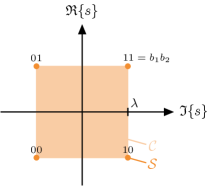
(a) QPSK           

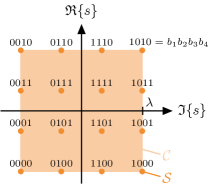
(b) 16-QAM           

Figure 3: Transmit constellations $\mathcal{S}$ (including the used Gray mapping) and their convex hulls $\mathcal{C}$. $\lambda=\sqrt{\nicefrac{{1}}{{2}}}$ for QPSK and $\lambda=\sqrt{\nicefrac{{9}}{{10}}}$ for 16-QAM.

TABLE I: LLR computation according to [47, Tbl. 1], [44]

	​​Bit $i$​​	$\ell(x)$
​QPSK​	$1$	$4\lambda\Re\{x\}$
	$2$	$4\lambda\Im\{x\}$
​16-QAM​	$1$	$\frac{2\lambda}{3}\left(4\Re\{x\}+\left|\Re\{x\}\!-\!\frac{2\lambda}{3}\right|-\left|\Re\{x\}\!+\!\frac{2\lambda}{3}\right|\right)\!$
	$2$	$\frac{4\lambda}{3}\left(\frac{2\lambda}{3}-\left|\Re\{x\}\right|\right)$
	$3$	$\frac{2\lambda}{3}\left(4\Im\{x\}+\left|\Im\{x\}\!-\!\frac{2\lambda}{3}\right|-\left|\Im\{x\}\!+\!\frac{2\lambda}{3}\right|\right)\!$
	$4$	$\frac{4\lambda}{3}\left(\frac{2\lambda}{3}-\left|\Im\{x\}\right|\right)$

TABLE II: Mapping the probabilities in (35) to symbol estimates [44, 52]

	$\Re\{\hat{s}\}$​	$\Im\{\hat{s}\}$
QPSK	$\lambda(2p_{1}-1)$	$\lambda(2p_{2}-1)$
16-QAM	${\color[rgb]{0,0,0}\frac{\lambda}{3}}(2p_{1}-1)(3-2p_{2})$	${\color[rgb]{0,0,0}\frac{\lambda}{3}}(2p_{3}-1)(3-2p_{4})$

We implement the unfolded algorithm in TensorFlow [49]. As loss function, we use the empirical binary cross-entropy (BCE) on the training set $\mathcal{D}$ between the transmitted bits and the estimated bit probabilities (35) from the last iteration as the output of our network. The loss as a function of the weights $\bm{\theta}=\{\tau^{(t)},\gamma^{(t)},\alpha^{(t)},\rho^{(t)}\}_{t=0}^{t_{\max}}$ is therefore

$$\!\!\!\!\mathcal{L}(\bm{\theta})=\!\sum_{d=1}^{|\mathcal{D}|}\beta^{(d)}\!\!\!\sum_{i=1}^{\log_{2}\!|\mathcal{S}|}\!\sum_{u=1}^{U}\sum_{k=T+1}^{K}\!\!\!\text{BCE}\!\left(b_{i,u,k}^{(d)},\Big{(}\!p_{i,u,k}^{(t_{\max})}\!\Big{)}^{\!\!(d)}\right)\!,\!\!\!$$ (37)

where

$$\text{BCE}(b,p)=b\log_{2}(p)+(1-b)\log_{2}(1-p),$$ (38)

and where $\beta^{(d)}$ are the weights given to the different samples in the training set $\mathcal{D}$ (see below). The dependence on the right-hand-side of (37) on the parameters $\bm{\theta}$ is through the bit probabilites $p_{i,u,k}^{(t_{\max})}$ which are functions of $\bm{\theta}$.

We only learn a single set of weights per system dimensions $\{U,B,K\}$, which is used for all signal-to-noise ratios (SNRs) and, most importantly, all jamming attacks (since a receiver does not typically know in advance which type of a jamming attack it is facing). For this reason, we train using a training set $\mathcal{D}$ which contains samples from different SNRs and different jamming attacks. We also have to avoid overfitting to a specific type of jamming attack. If our evaluation in sec:results would feature only the exact same types of jammers that were used for training, this would raise questions about the ability of SO-MAED to generalize to jamming attacks which differ from those explicitly included in the training set. However, the principles underlying the SO-MAED algorithm are essentially invariant with respect to the type of a jamming attack. For this reason, we only train on a single type of jammers, namely pilot jammers, cf. sec:setup (which we have empirically recognized to be the most difficult to mitigate), while evaluating the trained algorithm on many other jammer types besides pilot jammers, cf. sec:results. The attacks used for training also comprise different jammer receive strengths, namely $\{-\infty\,\text{dB},0\,\text{dB},10\,\text{dB},20\,\text{dB},40\,\text{dB},80\,\text{dB}\}$ relative to the average UE.

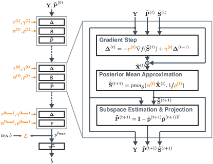
Figure 4: A graphical illustration of the neural network which implements the SO-MAED algorithm. The trainable parameters are depicted in orange. Also in orange is the loss function $\mathcal{L}$ (cf. (37)) which is used for training and which has as inputs the ground-truth transmitted information bits $b$ of the training set $\mathcal{D}$, as well as their respective probabilistic estimates $p^{t_{\max}}$.

The sample weights $\beta^{(d)}$ are used to prevent certain training samples (e.g., those at low SNR with strong jammers) from dominating the learning process by drowning out the loss contribution of training samples with inherently lower BCE. For this, we fix a baseline performance and select the weight $\beta^{(d)}$ of a training sample as the inverse of this sample’s BCE loss according to the baseline. The baseline performance is set by an untrained version of SO-MAED with reasonably initialized weights $\bm{\theta}$ (its performance in general already exceeds that of MAED).

For training, we use the Adam optimizer [53] from Keras with default values[54]. Training starts with a batch size of one sample, but the batch size is increased (first to five, then to ten, and finally to twenty samples) whenever the training loss does not improve for two consecutive epochs.

For a more extensive discussion on deep learning architectures in communication transceivers, we refer to [55, 56].

Algorithm 2 SO-MAED

1:input: $\mathbf{Y},\{\tau^{(t)},\alpha^{(t)},{\color[rgb]{0,0,0}\gamma^{(t)}},\rho^{(t)}\}_{t=0}^{t_{\max}-1}$

2:$\tilde{}\mathbf{S}^{(0)}\!=\!\left[\mathbf{S}_{T},\mathbf{0}_{U\!\times\!D}\right],\tilde{}\mathbf{p}^{(0)}\!=\!\mathbf{v}_{1}(\mathbf{Y}\mathbf{Y}^{\text{H}}\!+\mathbf{\Gamma}),\mathbf{\Delta}^{(-1)}=\mathbf{0}$

3:$\tilde{}\mathbf{P}^{(0)}=\mathbf{I}_{B}-\tilde{}\mathbf{p}^{(0)}\tilde{}\mathbf{p}^{(0)}{}^{\text{H}}$

4:for $t=0$ to $t_{\max}-1$ do

5:   $\nabla f(\tilde{}\mathbf{S}^{(t)})=-\big{(}\mathbf{Y}\tilde{}\mathbf{S}^{(t)}{}^{\dagger}\big{)}^{\text{H}}\tilde{}\mathbf{P}^{(t)}\mathbf{Y}(\mathbf{I}_{K}-\tilde{}\mathbf{S}^{(t)}{}^{\dagger}\tilde{}\mathbf{S}^{(t)})$

6:   $\mathbf{\Delta}^{(t)}=-\tau^{(t)}\nabla f(\tilde{}\mathbf{S}^{(t)})+{\color[rgb]{0,0,0}\gamma^{(t)}}\mathbf{\Delta}^{(t-1)}$

7:   $\tilde{}\mathbf{X}^{(t)}=\tilde{}\mathbf{S}^{(t)}+\mathbf{\Delta}^{(t)}$

8:   $\tilde{}\mathbf{S}^{(t+1)}=\text{pma}_{\mathcal{S}}\big{(}\alpha^{(t)}\tilde{}\mathbf{X}^{(t)},1/\rho^{(t)}\big{)}$

9:   $\tilde{}\mathbf{E}^{(t+1)}=\mathbf{Y}(\mathbf{I}_{K}-\tilde{}\mathbf{S}^{(t+1)}{}^{\dagger}\tilde{}\mathbf{S}^{(t+1)})$

10:   $\tilde{}\mathbf{p}^{(t+1)}=\tilde{}\mathbf{E}^{(t+1)}\tilde{\mathbf{E}}^{(t+1)}{}^{\text{H}}\,\tilde{}\mathbf{p}^{(t)}/\|\tilde{}\mathbf{E}^{(t+1)}\tilde{\mathbf{E}}^{(t+1)}{}^{\text{H}}\,\tilde{}\mathbf{p}^{(t)}\|_{2}$

11:   $\tilde{}\mathbf{P}^{(t+1)}=\mathbf{I}_{B}-\tilde{}\mathbf{p}^{(t+1)}\tilde{}\mathbf{p}^{(t+1)}{}^{\text{H}}$

12:end for

13:output: $\tilde{}\mathbf{S}^{(t_{\max})}_{[T+1:K]}$

VII Simulation Results

VII-A Simulation Setup

We simulate a massive MU-MIMO system with $B=128$ BS antennas, $U=32$ single-antenna UEs, and one single-antenna jammer. The UEs transmit for $K=160$ time slots, where the first $T=32$ slots are used for orthogonal pilots $\mathbf{S}_{T}$ in the form of a $32\times 32$ Hadamard matrix with unit symbol energy. The remaining $D=128$ slots are used to transmit QPSK or 16-QAM payload data. Unless noted otherwise, the channels are modelled as i.i.d. Rayleigh fading. We define the average receive signal-to-noise ratio (SNR) as

$$\textit{SNR}\triangleq\frac{\operatorname{\mathbb{E}}_{\mathbf{S}}\mathopen{}\left[\|\mathbf{H}\mathbf{S}\|_{F}^{2}\right]}{\operatorname{\mathbb{E}}_{\mathbf{N}}\mathopen{}\left[\|\mathbf{N}\|_{F}^{2}\right]}.$$ (39)

We consider four different jammer types: (J1) barrage jammers that transmit i.i.d. jamming symbols during the entire coherence interval, (J2) pilot jammers that transmit i.i.d. jamming symbols during the pilot phase but do not jam the data phase, (J3) data jammers that transmit i.i.d. jamming symbols during the data phase but do not jam the pilot phase, and (J4) sparse jammers that transmit i.i.d. jamming symbols during some fraction $\alpha$ of randomly selected bursts of unit length (i.e., one time slot). The jamming symbols are either circularly symmetric complex Gaussian or drawn uniformly from the transmit constellation (i.e., QPSK or 16-QAM). They are also independent of the UE transmit symbols $\mathbf{S}$, unless stated otherwise. We quantify the strength of the jammer’s interference relative to the strength of the average UE, either as the ratio between total receive energy

$$\rho_{\textsf{\tiny{E}}}\triangleq\frac{\operatorname{\mathbb{E}}_{\mathbf{w}}\mathopen{}\left[\|\mathbf{j}\mathbf{w}\|_{2}^{2}\right]}{\frac{1}{U}\operatorname{\mathbb{E}}_{\mathbf{S}}\mathopen{}\left[\|\mathbf{H}\mathbf{S}\|_{F}^{2}\right]},$$ (40)

or as the ratio between receive power during those phases that the jammer is jamming

$$\rho_{\textsf{\tiny{P}}}\triangleq\frac{\rho_{\textsf{\tiny{E}}}}{\gamma},$$ (41)

where $\gamma$ is the jammer’s duty cycle and equals $1,\frac{T}{K},\frac{D}{K}$, or $\alpha$ for barrage, pilot, data, or sparse jammers, respectively. This allows us to either precisely control the jammer energy (for jammers which are assumed to be essentially energy-limited) or the transmit intensity (for jammers which may want to pass themselves off as a legitimate UE, for instance).

VII-B Performance Baselines

We set the number of iterations for MAED and SO-MAED to $t_{\max}=20$ and emphasize again that we use only two different sets of weights for SO-MAED: one for QPSK transmission and one for 16-QAM transmission. Neither SO-MAED nor MAED is adapted to the different jammer scenarios. We compare our algorithms to the following baseline methods: The first baseline is the “LMMSE” method from sec:example, which does not mitigate the jammer and separately performs least-squares (LS) channel estimation and LMMSE data detection. The second baseline is the “geniePOS” method from sec:example, which projects the receive signals onto the orthogonal complement of the true jammer subspace and then separately performs LS channel estimation and LMMSE data detection in this projected space. The last baseline, “JL-SIMO,” serves as a bound for attainable error-rate performance. This method operates in a jammerless but otherwise equivalent system and implements (with perfect channel knowledge) the single-input multiple-output (SIMO) bound corresponding to the idealized case in which no inter-user interference is present.

​​​​​ ​​ ​​ ​​ ​​

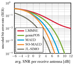
(a) strong barrage jammer (J1)

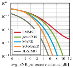
(b) strong pilot jammer (J2)

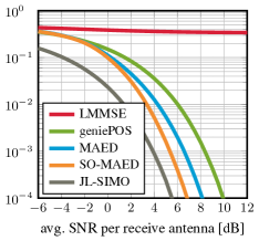
(c) strong data jammer (J3)

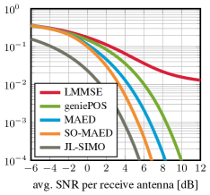
(d) strong sparse jammer (J4)

Figure 5: Uncoded bit error-rate (BER) for QPSK transmission in the presence of a strong ($\rho_{\textsf{\tiny{E}}}=30$ dB) jammer which transmits Gaussian symbols (a) during the entire coherence interval, (b) during the pilot phase only, (c) during the data phase only, or (d) in random unit-symbol bursts with a duty cycle of $\alpha=20\%$.

​​​​​ ​​ ​​ ​​ ​​

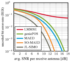
(a) strong barrage jammer (J1)

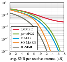
(b) strong pilot jammer (J2)

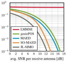
(c) strong data jammer (J3)

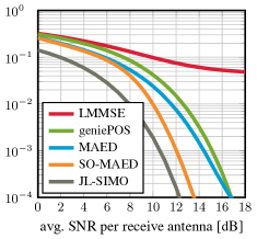
(d) strong sparse jammer (J4)

Figure 6: Uncoded bit error-rate (BER) for 16-QAM transmission in the presence of a strong ($\rho_{\textsf{\tiny{E}}}\!=\!30$ dB) jammer which transmits Gaussian symbols (a) during the entire coherence interval, (b) during the pilot phase only, (c) during the data phase only, or (d) in random unit-symbol bursts with a duty cycle of $\alpha=20\%$.

​​​​​ ​​ ​​ ​​ ​​

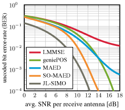
(a) weak barrage jammer (J1)

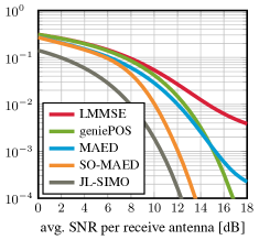
(b) weak pilot jammer (J2)

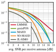
(c) weak data jammer (J3)

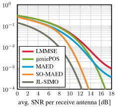
(d) weak sparse jammer (J4)

Figure 7: Uncoded bit error-rate (BER) for 16-QAM transmission in the presence of a weak ($\rho_{\textsf{\tiny{P}}}=0$ dB) jammer which transmits 16-QAM symbols (a) during the entire coherence interval, (b) during the pilot phase only, (c) during the data phase only, or (d) in random unit-symbol bursts with a duty cycle of $\alpha=20\%$.

​​​​​ ​​ ​​ ​​ ​​

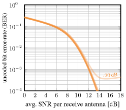
(a) barrage jammers (J1)

(b) pilot jammers (J2)

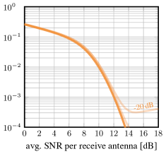
(c) data jammers (J3)

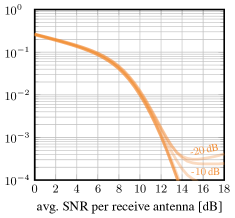
(d) sparse jammers (J4)

Figure 8: Uncoded bit error-rate (BER) performance curves of SO-MAED in the presence of jammers with different receive powers compared to the average UE, $\rho_{\textsf{\tiny{P}}}\in\{-20\,\text{dB},-10\,\text{dB},0\,\text{dB},10\,\text{dB},20\,\text{dB},40\,\text{dB},80\,\text{dB}\}$. The subfigures correspond to the different jammer types (J1) - (J4) and show one curve per jammer power (plotted with 25% opacity to depict the degree of overlap between curves). Curves that level off into an error floor are labeled with their jammer power, e.g., in fig:many:static, the barrage jammer with receive power $\rho_{\textsf{\tiny{P}}}=-20$ dB has an error floor while all other barrage jammers have virtually identical BER curves.

VII-C Mitigation of Strong Gaussian Jammers

We first investigate the ability of MAED and SO-MAED to mitigate strong jamming attacks. For this, we simulate Gaussian jammers with $\rho_{\textsf{\tiny{E}}}=30$ dB of all four types introduced in Section VII-A and evaluate the performance of our algorithms compared to the baselines of Section VII-B for QPSK transmission (fig:qpsk_strong_jammers) as well as for 16-QAM transmission (fig:strong_jammers). We note at this point that the performances of geniePOS and JL-SIMO are independent of the considered jammer type: geniePOS uses the genie-provided jammer channel to null the jammer perfectly, regardless of its transmit sequence, and JL-SIMO operates on a jammerless system. Unsurprisingly, the jammer-oblivious LMMSE baseline performs significantly worse than the jammer-robust geniePOS baseline under all attack scenarios, with the data jamming attack turning out to be the most harmful and the pilot jamming attack the least harmful. Both MAED and SO-MAED succeed in mitigating all four jamming attacks with highest effectiveness, even outperforming the genie-assisted geniePOS method by a considerable margin. Their efficacy is further reflected in the fact that SO-MAED and MAED approach the performance of the jammerless and MU interference-free JL-SIMO bound to within less than $2$ dB and $3$ dB at $0.1$% BER, respectively, in all considered scenarios.

The behavior is largely similar when 16-QAM instead of QPSK is used as transmit constellation (fig:strong_jammers). However, due to the decreased informativeness of the box prior for such higher-order constellations, MAED performs now closer to geniePOS, while SO-MAED still performs within $2$ dB (at $0.1$% BER) of the JL-SIMO bound. The increased performance gap between them notwithstanding, both MAED and SO-MAED are able to effectively mitigate all four attack types.

VII-D Mitigation of Weak Constellation Jammers

We now turn to the analysis of more restrained jamming attacks in which the jammer transmits constellation symbols with relative power $\rho_{\textsf{\tiny{P}}}=0$ dB during its on-phase (to pass itself off as just another UE, for instance [11]). Simulation results for 16-QAM transmission under all four types of jamming attacks are shown in fig:weak_jammers. Because of the weaker jamming attacks, the jammer-oblivious LMMSE baseline now performs closer to the jammer-resistant geniePOS baseline than it does in fig:strong_jammers. MAED again mitigates all attack types rather successfully, outperforming geniePOS in the low-SNR regime but slightly leveling off at high SNR. Interestingly, MAED shows worse performance under these weak jamming attacks than under the strong jamming attacks of fig:strong_jammers. The reason is the following: MAED searches for the jamming subspace by looking for the dominant dimension of the iterative residual error $\tilde{}\mathbf{E}^{(t)}$, see eq:rayleigh. If the received jamming energy is small compared to the received signal energy, then it becomes hard to distinguish the residual errors caused by the jamming signal from those caused by errors in estimating the channel and data matrices $\tilde{}\mathbf{H}_{\mathbf{P}}^{(t)}$ and $\tilde{}\mathbf{S}_{D}^{(t)}$. Note in contrast that, due to its superior signal prior, the equivalent performance loss of SO-MAED is only so small as to be virtually unnoticeable. Thus, SO-MAED outperforms MAED by a large margin and still approaches the JL-SIMO bound by less than 2dB at a BER of 0.1%.

VII-E How Universal is SO-MAED Really?

In the remainder of our evaluation, we focus mostly on SO-MAED, since it is clearly the better of the two proposed algorithms. To show that our approach indeed succeeds in mitigating arbitrary jamming attacks without need for fine-tuning of the algorithm or its parameters, fig:many_jammers depicts performance results for a series of jamming attacks spanning a dynamic range from $\rho_{\textsf{\tiny{P}}}=-20$ dB to $\rho_{\textsf{\tiny{P}}}=80$ dB. Specifically, fig:many_jammers shows results for all four jammer types, where every subfigure plots BER curves for jamming attacks with $\rho_{\textsf{\tiny{P}}}\in\{-20\,\text{dB},-10\,\text{dB},0\,\text{dB},10\,\text{dB},20\,\text{dB},40\,\text{dB},80\,\text{dB}\}$. The purpose of these plots is to illustrate that, apart from jamming attacks where the jammer is significantly weaker than the average UE, the curves are virtually indistinguishable, meaning that the performance of SO-MAED is essentially independent of the specific type of jamming attack that it is facing.

VII-F Eclipsed Jammers

​​​​​ ​​​​​ ​​
​​​​​​ ​​​ ​​

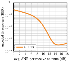
(a) no jammer

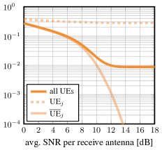
(b) weak UE-impersonating jammer

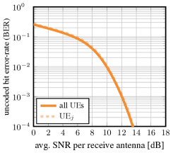
(c) strong UE-impersonating jammer

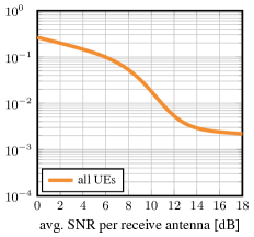
(d) data-dependent jammer

Figure 9: Uncoded bit error-rate of SO-MAED for different types of eclipsed jammers: (a) no jammer, (b) $\rho_{\textsf{\tiny{P}}}=0$ dB jammer impersonating the $j$th UE by transmitting its pilot sequence ($\text{UE}_{j}$ denotes the BER of the impersonated UE, and $\overline{\text{UE}}_{j}$ the BER among all other UEs), (c) $\rho_{\textsf{\tiny{P}}}=30$ dB jammer impersonating the $j$th UE by transmitting its pilot sequence, and (d) jammer causes eclipsing by transmitting a jamming sequence that depends on the UE transmit matrix $\mathbf{S}$. Dashed lines represent the BER of the impersonated UE, transparent lines represent the BER among the UEs that are not impersonated by the jammer.

Up to this point, the jamming signal $\mathbf{w}$ has always been independent of the UE transmit matrix $\mathbf{S}$. The strong performance results of both MAED and SO-MAED have supported the claim in Remark 2 that, in this case, eclipsing is the (rare) exception, not the norm. We now turn to an empirical analysis of how SO-MAED behaves when eclipsing does occur (fig:eclipsed). To this end, we consider scenarios in which the jammer is eclipsed because there is no jamming activity (fig:eclipsed:no_jam), because the jammer transmits a UE’s pilot sequence (fig:eclipsed:weak_impers, fig:eclipsed:strong_impers), or because the jamming sequence $\mathbf{w}$ depends on the transmit matrix $\mathbf{S}$ (which in reality would be unknown to the jammer) in a way that causes eclipsing (fig:eclipsed:row_eclipsed).

In the case of no jammer (fig:eclipsed:no_jam), or no jamming activity within a coherence interval, we see that SO-MAED still reliably detects the transmit data. However, our method now suffers from an error floor (albeit significantly below $0.1$% BER). The reason for this error floor is that, in the absence of jamming energy to guide the choice of the nulled direction $\tilde{}\mathbf{p}$, there is the temptation to instead “cover up” detection errors (similar to the phenomenon discussed in sec:results:weak). However, the low level of the error floor shows that this potential pitfall does not cause a systematic breakdown of SO-MAED. We emphasize also that SO-MAED does not simply null the strongest UE. Such (degenerate) behavior would only occur if one UE were far stronger than the others. With any reasonable power control scheme, UE nulling is not an issue. In the case of a jammer that impersonates the $j$th UE by transmitting its pilot sequence in the training phase and constellation symbols in the data phase, with the same power as the average UE ($\rho_{\textsf{\tiny{P}}}=0$ dB), SO-MAED indeed suffers a performance breakdown (fig:eclipsed:weak_impers). However, closer inspection shows that this error floor is caused solely by errors in detecting the symbols of the impersonated UE. This is not surprising: The jammer is statistically indistinguishable from the $j$th UE, so that is impossible to reliably separate the UE transmit symbols from the fake jammer transmit symbols. In this regard, we refer again to the information-theoretic discussion of [43, Sec. V]. Such impersonation attacks could be forestalled by using encrypted pilots [57]. If the jammer transmits the $j$th UE’s pilot sequence and constellation symbols, but with much more power ($\rho_{\textsf{\tiny{P}}}=30$ dB), then the iterative detection procedure of SO-MAED will separate the jammer subspace from the $j$th UE’s subspace (fig:eclipsed:strong_impers), since, being so much stronger than any UE, the jammer subspace will dominate the residual matrix $\tilde{}\mathbf{E}^{(t)}$ in eq:rayleigh. Finally, fig:eclipsed:row_eclipsed shows results for a case where the jammer knows $\mathbf{S}$ and selects an $\tilde{}\mathbf{S}_{D}$ which differs from $\mathbf{S}_{D}$ in a single row (with valid constellation symbols in the differing row), so that $\textit{rank}(\mathbf{S}_{D}-\tilde{}\mathbf{S}_{D})=1$. It then draws $\mathbf{w}_{T}\sim\mathcal{C}\mathcal{N}(\mathbf{0},\mathbf{I}_{D})$ and sets $\mathbf{w}_{D}^{\text{T}}=\mathbf{w}_{T}^{\text{T}}\mathbf{S}_{T}^{\dagger}\tilde{\mathbf{S}}_{D}$ to cause eclipsing (cf. def:eclipse). The jammer strength is $\rho_{\textsf{\tiny{P}}}=30$ dB. The results show an error floor at roughly 0.2% BER caused by the presence of an alternative spurious solution. However, the results in Figs. 5 – 8 show that when the jammer has to select $\mathbf{w}$ without knowing $\mathbf{S}_{D}$—which will be the case in most practical scenarios, as we argued in sec:limitations—, such accidental eclipsing is extremely rare.

VII-G Beyond i.i.d. Rayleigh Fading

So far, our experiments were based on i.i.d. Rayleigh fading channels, but our method does not depend in any way on this particular channel model. To demonstrate that MAED and SO-MAED are also applicable in scenarios that deviate strongly from the i.i.d. Rayleigh model and that exhibit significant correlations between the jammer’s and the UEs’ channels, we now evaluate our algorithms on mmWave channels generated with the commercial Wireless InSite ray-tracer [58]. The simulated scenario is depicted in fig:remcom_scenario. We simulate a mmWave massive MU-MIMO system with a carrier frequency of $60$ GHz and a bandwidth of $100$ MHz. The BS is placed at a height of $10$ m and consists of a horizontal uniform linear array with $B=128$ omnidirectional antennas spaced at half a wavelength. The omnidirectional single-antenna UEs and the jammer are located at a height of $1.65$ m and placed in a $150^{\circ}$ sector spanning $180$ m$\times$$90$ m in front of the BS; see fig:remcom_scenario. The UEs and the jammer are drawn at random from a grid with $5$ m pitch while ensuring that the minimum angular separation between any two UEs, as well as between the jammer and any UE, is $2.5^{\circ}$. We assume $\pm 1.5$ dB power control, so that the ratio between the maximum and minimum per-UE receive power is 2.

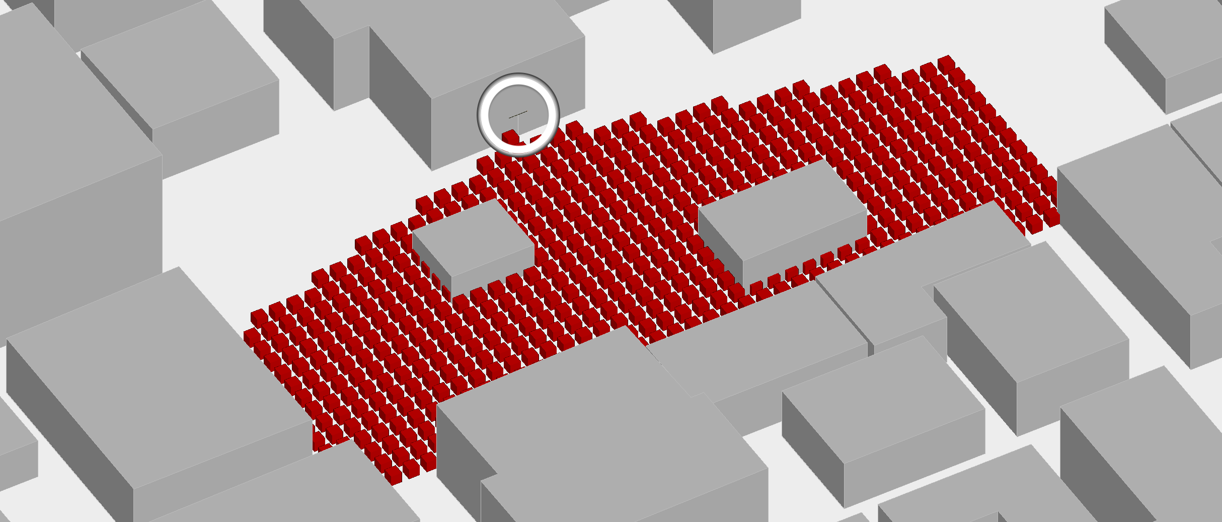
Figure 10: Simulated scenario. The location of the BS his highlighted by the white circle while the red squares depict all possible UE locations.

​​​​​ ​​​ ​​
​​​​​ ​​​ ​​

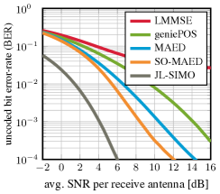
(a) barrage jammer (J1)

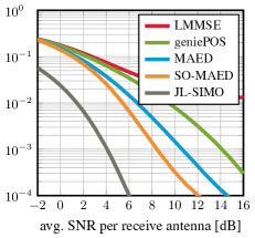
(b) pilot jammer (J2)

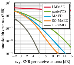
(c) data jammer (J3)

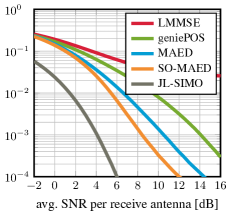
(d) sparse jammer (J4)

Figure 11: Uncoded bit error-rate (BER) for QPSK transmission over realistic mmWave channels in the presence of a strong ($\rho_{\textsf{\tiny{E}}}=30$ dB) jammer.

The high correlation exhibited by these mmWave channels slows convergence of MAED and SO-MAED, so we increase their number of iterations to $t_{\max}=30$. We also retrain the parameters from SO-MAED on mmWave channels (while making a clear split between the training set and the evaluation set).

The results for QPSK transmission in the presence of $\rho_{\textsf{\tiny{E}}}=30$ dB are shown in fig:remcom_results. The performance hierarchy is identical as in the equivalent Rayleigh-fading setup of fig:qpsk_strong_jammers: geniePOS is clearly outperformed by MAED, which is in turn outperformed by SO-MAED. However, the more challenging nature of mmWave channels amplifies performance differences: Due to its artificial immunity from the high inter-user interference of mmWave channels, JL-SIMO is now in a class of its own. However, MAED and SO-MAED gain almost $4$ dB and $6$ dB in SNR on geniePOS at $0.1\%$ BER, respectively, regardless of the jammer type. This shows that MAED and SO-MAED are also well suited for scenarios that deviate significantly from the i.i.d. Rayleigh model.

VIII Conclusions

We have proposed a method for the mitigation of smart jamming attacks on the massive MU-MIMO uplink and supported its basic soundness with theoretical results. In contrast to existing mitigation methods, our approach does not rely on jamming activity during any particular time instant. Instead, our method utilizes a newly proposed problem formulation which exploits the fact that the jammer’s subspace remains constant within a coherence interval. We have developed two efficient iterative algorithms, MAED and SO-MAED, which approximately solve the proposed optimization problem. Our simulation results have shown that MAED and SO-MAED are able to effectively mitigate a wide range of jamming attacks. In particular, they succeed in mitigating attack types like data jamming and sparse jamming, for which—to the best of our knowledge—no mitigation methods have existed so far.

There are numerous avenues for future work. Of particular importance is the development of methods for synchronization in the presence of smart jammers. Another issue is the question of how to obtain the required channel state information for transmit beamforming in the case of multi-antenna UEs and point-to-point MIMO. Finally, our method focuses on the massive MIMO uplink. Equally important is, of course, the downlink, which presents the additional difficulty that UEs would probably only be able to rely on hybrid beamforming. Since MAED and SO-MAED presume fully digital beamforming, the development of hybrid beamformers to mitigate smart jammers is therefore also a relevant problem for future work.

Appendix A Proof of thm:maed

Clearly, if $\{\hat{}\mathbf{p},\hat{}\mathbf{H}_{\mathbf{P}},\hat{}\mathbf{S}_{D}\}=\{\mathbf{p},\mathbf{P}\mathbf{H},\mathbf{S}_{D}\}$, then

$$\hat{}\mathbf{P}\mathbf{Y}-\hat{}\mathbf{H}_{\mathbf{P}}\hat{}\mathbf{S} =\mathbf{P}\mathbf{Y}-\mathbf{P}\mathbf{H}\mathbf{S}$$ (42)

$$=\mathbf{P}(\mathbf{H}\mathbf{S}+\mathbf{j}\mathbf{w}^{\text{T}})-\mathbf{P}\mathbf{H}\mathbf{S}$$ (43)

$$=\mathbf{P}\mathbf{j}\mathbf{w}^{\text{T}}=\mathbf{0},$$ (44)

and so the objective (12) is zero. Since the objective function is nonnegative, it follows that $\{\hat{}\mathbf{p},\hat{}\mathbf{H}_{\mathbf{P}},\hat{}\mathbf{S}_{D}\}=\{\mathbf{p},\mathbf{P}\mathbf{H},\mathbf{S}_{D}\}$ is a solution to (12). It remains to prove uniqueness. For this, we rewrite the objective in (12) as

$$\big{\|}\tilde{}\mathbf{P}\mathbf{Y}-\tilde{}\mathbf{H}_{\mathbf{P}}\tilde{}\mathbf{S}\big{\|}^{2}_{F}$$

$$=\big{\|}\tilde{}\mathbf{P}\mathbf{Y}_{T}-\tilde{}\mathbf{H}_{\mathbf{P}}\mathbf{S}_{T}\big{\|}^{2}_{F}+\big{\|}\tilde{}\mathbf{P}\mathbf{Y}_{D}-\tilde{}\mathbf{H}_{\mathbf{P}}\tilde{}\mathbf{S}_{D}\big{\|}^{2}_{F}.$$ (45)

The objective can only be zero if both terms on the right-hand-side (RHS) of (45) are zero. The first term is zero if and only if

$$\tilde{}\mathbf{P}\mathbf{Y}_{T}-\tilde{}\mathbf{H}_{\mathbf{P}}\mathbf{S}_{T}=\mathbf{0},$$ (46)

which implies

$$\tilde{}\mathbf{H}_{\mathbf{P}}=\tilde{}\mathbf{P}\mathbf{Y}_{T}\mathbf{S}_{T}^{\dagger},$$ (47)

since $\mathbf{S}_{T}$ has full row rank. Plugging this back into the second term on the RHS of (45) gives

$$\tilde{}\mathbf{P}\mathbf{Y}_{D}-\tilde{}\mathbf{H}_{\mathbf{P}}\tilde{}\mathbf{S}_{D}$$ (48)

$$=\tilde{}\mathbf{P}(\mathbf{Y}_{D}-\mathbf{Y}_{T}\mathbf{S}_{T}^{\dagger}\tilde{}\mathbf{S}_{D})$$ (49)

$$=\tilde{}\mathbf{P}\left(\mathbf{H}\mathbf{S}_{D}+\mathbf{j}\mathbf{w}_{D}^{\text{T}}-(\mathbf{H}\mathbf{S}_{T}+\mathbf{j}\mathbf{w}_{T}^{\text{T}})\mathbf{S}_{T}^{\dagger}\tilde{}\mathbf{S}_{D}\right)$$ (50)

$$=\tilde{}\mathbf{P}\left(\mathbf{H}[\mathbf{S}_{D}-\tilde{}\mathbf{S}_{D}]+\mathbf{j}[\mathbf{w}_{D}^{\text{T}}-\mathbf{w}_{T}^{\text{T}}\mathbf{S}_{T}^{\dagger}\tilde{}\mathbf{S}_{D}]\right).$$ (51)

The second term on the RHS of (45) (and, hence, the objective) is zero if and only if the matrix in (51) is the zero matrix. The projector $\tilde{\mathbf{P}}$ can null a matrix of (at most) rank one. It follows that the objective function in (45) can be zero only if

$$\mathbf{H}[\mathbf{S}_{D}-\tilde{}\mathbf{S}_{D}]+\mathbf{j}[\mathbf{w}_{D}^{\text{T}}-\mathbf{w}_{T}^{\text{T}}\mathbf{S}_{T}^{\dagger}\tilde{}\mathbf{S}_{D}]$$ (52)

is a matrix of (at most) rank one. Since $\mathbf{H}$ has full column rank and, by assumption, $\mathbf{j}$ is not included in the column space of $\mathbf{H}$, this requires that the matrix $[\mathbf{S}_{D}-\tilde{}\mathbf{S}_{D};\mathbf{w}_{D}^{\text{T}}-\mathbf{w}_{T}^{\text{T}}\mathbf{S}_{T}^{\dagger}\tilde{}\mathbf{S}_{D}]$ has rank one. By our assumption that the jammer is not eclipsed, this can only happen if $\tilde{}\mathbf{S}_{D}=\mathbf{S}_{D}$, so the estimated data matrix coincides with the true data matrix. In that case, (51) is

$$\tilde{}\mathbf{P}\mathbf{j}[\mathbf{w}_{D}^{\text{T}}-\mathbf{w}_{T}^{\text{T}}\mathbf{S}_{T}^{\dagger}\tilde{}\mathbf{S}_{D}],$$ (53)

which (again by the assumption that the jammer is not eclipsed) is zero if and only if $\tilde{}\mathbf{p}$ is collinear with $\mathbf{j}$, meaning that $\tilde{}\mathbf{p}=\alpha\mathbf{p},|\alpha|=1$. This means that also the estimated jammer subspace coincides with the true jammer subspace. Finally, plugging this value of $\tilde{}\mathbf{p}$ back into (47) yields

$$\tilde{}\mathbf{H}_{\mathbf{P}} =\tilde{}\mathbf{P}\mathbf{Y}_{T}\mathbf{S}_{T}^{\dagger}$$ (54)

$$=\tilde{}\mathbf{P}(\mathbf{H}\mathbf{S}_{T}+\mathbf{j}\mathbf{w}_{T}^{\text{T}})\mathbf{S}_{T}^{\dagger}$$ (55)

$$=\tilde{}\mathbf{P}\mathbf{H}\mathbf{S}_{T}\mathbf{S}_{T}^{\dagger}=\mathbf{H}_{\mathbf{P}},$$ (56)

showing that also the estimated channel matrix coincides with the projection of the true channel matrix. We have thereby shown that $\big{\|}\tilde{}\mathbf{P}\mathbf{Y}-\tilde{}\mathbf{H}_{\mathbf{P}}\tilde{}\mathbf{S}\big{\|}^{2}_{F}$ is zero if and only if $\tilde{}\mathbf{S}_{D}=\mathbf{S}_{D}$, $\tilde{}\mathbf{p}=\alpha\mathbf{p},|\alpha|=1$, and $\tilde{}\mathbf{H}_{\mathbf{P}}=\mathbf{H}_{\mathbf{P}}$. $\blacksquare$

Appendix B Proof of thm:maed2

$\mathbf{S}_{T}$ is unitary, so $\mathbf{S}_{T}^{\dagger}=\mathbf{S}_{T}^{\text{H}}$. The jammer eclipses if there exists a matrix $\tilde{}\mathbf{S}_{D}\in\mathcal{S}^{U\times D},\tilde{}\mathbf{S}_{D}\neq\mathbf{S}_{D}$ such that the matrix

$$\bm{\Sigma}=\begin{bmatrix}\mathbf{S}_{D}-\tilde{}\mathbf{S}_{D}\\ \mathbf{w}_{D}^{\text{T}}-\mathbf{w}_{T}^{\text{T}}\mathbf{S}_{T}^{\text{H}}\tilde{\mathbf{S}}_{D}\end{bmatrix}$$ (57)

has rank one, meaning that

$$\begin{bmatrix}\mathbf{S}_{D}-\tilde{}\mathbf{S}_{D}\\ \mathbf{w}_{D}^{\text{T}}-\mathbf{w}_{T}^{\text{T}}\mathbf{S}_{T}^{\text{H}}\tilde{\mathbf{S}}_{D}\end{bmatrix}=\begin{bmatrix}\mathbf{a}\\ \alpha\end{bmatrix}\mathbf{b}^{\text{T}}$$ (58)

for some $\mathbf{a}\in\mathbb{C}^{U},\mathbf{b}\in\mathbb{C}^{D},\alpha\in\mathbb{C}$. Whether such an $\tilde{}\mathbf{S}_{D}$ exists depends on the realization of the random matrices $\mathbf{S}_{D}$ and $\mathbf{S}_{T}$.
We now decompose the probability that an $\tilde{}\mathbf{S}_{D}$ exists for which (58) holds (i.e., the probability that the jammer eclipses) into the sum of the probability that such an $\tilde{}\mathbf{S}_{D}$ exists which has rank one, plus the probability that such an $\tilde{}\mathbf{S}_{D}$ exists whose rank exceeds one. The proof proceeds by showing that the probability of the first of these two events is “small,” and that the probability of the second event is zero.
We start by bounding the probability that there exists a rank-one $\tilde{}\mathbf{S}_{D}$ which satisfies (58). Clearly, this probability is bounded by the probability that there exists a rank-one $\tilde{}\mathbf{S}_{D}$ which satisfies $\mathbf{S}_{D}-\tilde{}\mathbf{S}_{D}=\mathbf{a}\mathbf{b}^{\text{T}}$ for some $\mathbf{a}\in\mathbb{C}^{U},\mathbf{b}\in\mathbb{C}^{D}$. The entries of $\mathbf{S}_{D}-\tilde{}\mathbf{S}_{D}$ lie within the set

$$\Delta\mathcal{S}\triangleq\{s-\tilde{s}\,:\,s,\tilde{s}\in\mathcal{S}\}.$$ (59)

Without loss of generality, any rank-one matrix $\mathbf{S}_{D}-\tilde{}\mathbf{S}_{D}$ can therefore be represented by choosing the entries of the vectors $\mathbf{a}$ and $\mathbf{b}$ from sets with cardinality $|\Delta\mathcal{S}|\leq|\mathcal{S}|^{2}$. For instance, one could pick the entries of $\mathbf{b}$ from $\Delta\mathcal{S}$, and the entries of $\mathbf{a}$ would have to come from at most $|\Delta\mathcal{S}|$ different scaling factors. Analogously, $\tilde{}\mathbf{S}_{D}$ was assumed to be of rank one, $\tilde{}\mathbf{S}_{D}=\mathbf{c}\mathbf{d}^{\text{T}}$, and since the entries of $\tilde{}\mathbf{S}_{D}$ have to lie within $\mathcal{S}$, we can without loss of generality restrict the entries of $\mathbf{c},\mathbf{d}$ to lie within sets of cardinality $|\mathcal{S}|$. We may thus write

$$\mathbf{S}_{D}-\tilde{}\mathbf{S}_{D}=\mathbf{S}_{D}-\mathbf{c}\mathbf{d}^{\text{T}}=\mathbf{a}\mathbf{b}^{\text{T}}.$$ (60)

Thus, to cause eclipsing, a rank-one $\mathbf{S}_{D}$ would need to have the form

$$\mathbf{S}_{D}=\mathbf{a}\mathbf{b}^{\text{T}}+\mathbf{c}\mathbf{d}^{\text{T}}.$$ (61)

Since all $|\mathcal{S}|^{UD}$ possible realizations of $\mathbf{S}_{D}$ are equiprobable, the probability of (61) being satisfied can be bounded by bounding the number of different matrices that have the structure of (61). There are at most $|\mathcal{S}|^{2U}$ different choices for $\mathbf{a}$, at most $|\mathcal{S}|^{2D}$ different choices for $\mathbf{b}$, at most $|\mathcal{S}|^{U}$ different choices for $\mathbf{c}$, and at most $|\mathcal{S}|^{D}$ different choices for $\mathbf{d}$. In total, there are therefore at most $|\mathcal{S}|^{3U+3D}$ different matrices that have the form (61), and hence at most $|\mathcal{S}|^{3U+3D}$ different realizations of $\mathbf{S}_{D}$ for which there exists a rank-one $\tilde{}\mathbf{S}_{D}$ that causes eclipsing. Each of these realizations has probability $|\mathcal{S}|^{-UD}$, so the probability of eclipsing with a rank-one $\tilde{}\mathbf{S}_{D}$ can be bounded by

$$|\mathcal{S}|^{-UD}|\mathcal{S}|^{3U+3D}=|\mathcal{S}|^{3U}|\mathcal{S}|^{-(U-3)D}.$$ (62)

It remains to bound the probability that there exists an $\tilde{}\mathbf{S}_{D}$ whose rank exceeds one and which satisfies (58). For this, we consider the last row of (57) and define $\mathbf{x}\triangleq\mathbf{S}_{T}\mathbf{w}_{T}^{\ast}$. Since $\mathbf{S}_{T}$ is Haar distributed, $\mathbf{x}$ is distributed uniformly over the complex $U$-dimensional sphere of radius $\|\mathbf{w}_{T}\|_{2}$ [59, p. 16], which, by assumption, is greater than zero. Furthermore, $\mathbf{x}$ is independent of $\mathbf{w}_{D}$ and $\mathbf{S}_{D}$. We may therefore write $\mathbf{x}=\frac{\|\mathbf{w}_{T}\|_{2}}{\|\mathbf{z}\|_{2}}\mathbf{z}$, where the entries of $\mathbf{z}$ are i.i.d. circularly-symmetric complex Gaussians with unit variance, and where $\mathbf{z}$ is independent of $\mathbf{w}_{D}$ and $\mathbf{S}_{D}$. So we rewrite the last row as

$$\mathbf{w}_{D}^{\text{T}}-\mathbf{w}_{T}^{\text{T}}\mathbf{S}_{T}^{\text{H}}\tilde{\mathbf{S}}_{D}=\mathbf{w}_{D}^{\text{T}}-\frac{\|\mathbf{w}_{T}\|_{2}}{\|\mathbf{z}\|_{2}}\mathbf{z}^{\text{H}}\tilde{}\mathbf{S}_{D}.$$ (63)

Furthermore, for every $\mathbf{S}_{D}\in\mathcal{S}^{U\times D}$, we define the finite set

$$\mathcal{B}(\mathbf{S}_{D})\triangleq\big{\{}\mathbf{b}\!\in\!\Delta\mathcal{S}^{D}\,:\, \exists\tilde{}\mathbf{S}_{D}\!\in\!\mathcal{S}^{U\times D}\!\setminus\!\{\mathbf{S}_{D}\}\,\exists\mathbf{a}\!\in\!\mathbb{C}^{U}$$

$$\text{such that }\mathbf{S}_{D}-\tilde{}\mathbf{S}_{D}=\mathbf{a}\mathbf{b}^{\text{T}}\big{\}}.$$ (64)

The probability that there exists an $\tilde{}\mathbf{S}_{D}$ whose rank exceeds one and which satisfies (58) can therefore be bounded by the probability that

$$\mathbf{w}_{D}^{\text{T}}-\frac{\|\mathbf{w}_{T}\|_{2}}{\|\mathbf{z}\|_{2}}\mathbf{z}^{\text{H}}\tilde{}\mathbf{S}_{D}\in\mathcal{B}(\mathbf{S}_{D})$$ (65)

for some $\tilde{}\mathbf{S}_{D}$ of rank greater than one. Using the union bound, we can in turn bound this probability by the sum (over all $\mathbf{b}\in\mathcal{B}(\mathbf{S}_{D})$) of probabilities that

$$\mathbf{w}_{D}^{\text{T}}-\frac{\|\mathbf{w}_{T}\|_{2}}{\|\mathbf{z}\|_{2}}\mathbf{z}^{\text{H}}\tilde{}\mathbf{S}_{D}=\mathbf{b}^{\text{T}},$$ (66)

which would imply that $\tilde{}\mathbf{S}_{D}^{\text{H}}\mathbf{z}^{\ast}$ is collinear with $\mathbf{w}_{D}-\mathbf{b}$. So we can further bound the probability by the sum (over $\mathbf{b}$) of probabilities that $\tilde{}\mathbf{S}_{D}^{\text{H}}\mathbf{z}^{\ast}$ is collinear with $\mathbf{w}_{D}-\mathbf{b}$ (note that $\tilde{}\mathbf{S}_{D}^{\text{H}}\mathbf{z}^{\ast}$ is independent of $\mathbf{w}_{D}-\mathbf{b}$). Remember that the entries of $\mathbf{z}$, and hence of $\mathbf{z}^{\ast}$, are i.i.d. circularly-symmetric complex Gaussians with unit variance. So $\tilde{}\mathbf{S}_{D}^{\text{H}}\mathbf{z}^{\ast}$ is a circularly-symmetric complex Gaussian vector with covariance matrix $\tilde{}\mathbf{S}_{D}^{\text{H}}\tilde{}\mathbf{S}_{D}$. And since $\tilde{}\mathbf{S}_{D}^{\text{H}}$ has at least two linearly independent rows (since $\tilde{}\mathbf{S}_{D}$ was assumed to be of rank greater than one), $\tilde{}\mathbf{S}_{D}^{\text{H}}\mathbf{z}^{\ast}$ has at least two imperfectly correlated entries. Hence, for any fixed $\mathbf{b}$, the probability that $\tilde{}\mathbf{S}_{D}^{\text{H}}\mathbf{z}^{\ast}$ is collinear with $\mathbf{w}_{D}-\mathbf{b}$ is zero. And since there are only finitely many different vectors $\mathbf{b}$ to consider, the probability that (65) holds is zero. In other words, the probability is zero that there exists a $\tilde{}\mathbf{S}_{D}$ whose rank exceeds one such that the jammer eclipses. From this, the result follows. $\blacksquare$

References

- [1] G. Marti and C. Studer, “Mitigating smart jammers in MU-MIMO via joint channel estimation and data detection,” in Proc. IEEE Int. Conf. Commun. (ICC), May 2022, pp. 1336–1342.
- [2] “Satellite-navigation systems such as GPS are at risk of jamming,” The Economist. [Online]. Available: https://www.economist.com/science-and-technology/2021/05/06/satellite-navigation-systems-such-as-gps-are-at-risk-of-jamming
- [3] J. Kosinski et al., “Top Gun: Maverick,” Paramount Pictures, 2022.
- [4] P. Popovski, “Ultra-reliable communication in 5G wireless systems,” in Proc. Int. Conf. 5G Ubiquitous Connectivity, Nov. 2014, pp. 146–151.
- [5] H. Pirayesh and H. Zeng, “Jamming attacks and anti-jamming strategies in wireless networks: A comprehensive survey,” IEEE Commun. Surveys Tuts., vol. 9, no. 2, pp. 767–809, 2022.
- [6] G. Marti, O. Castañeda, and C. Studer, “Jammer mitigation via beam-slicing for low-resolution mmWave massive MU-MIMO,” IEEE Open J. Circuits Syst., vol. 2, pp. 820–832, 2021.
- [7] Q. Yan, H. Zeng, T. Jiang, M. Li, W. Lou, and Y. T. Hou, “Jamming resilient communication using MIMO interference cancellation,” IEEE Trans. Inf. Forensics Security, vol. 11, no. 7, pp. 1486–1499, Jul. 2016.
- [8] W. Shen, P. Ning, X. He, H. Dai, and Y. Liu, “MCR decoding: A MIMO approach for defending against wireless jamming attacks,” in Proc. IEEE Conf. Commun. Netw. Security (CNS), Oct. 2014, pp. 133–138.
- [9] L. M. Hoang, J. A. Zhang, D. N. Nguyen, X. Huang, A. Kekirigoda, and K.-P. Hui, “Suppression of multiple spatially correlated jammers,” IEEE Trans. Veh. Technol., vol. 70, no. 10, pp. 10 489–10 500, 2021.
- [10] H. Zeng, C. Cao, H. Li, and Q. Yan, “Enabling jamming-resistant communications in wireless MIMO networks,” in Proc. IEEE Conf. Commun. Netw. Security (CNS), Oct. 2017, pp. 1–9.
- [11] J. Vinogradova, E. Björnsson, and E. G. Larsson, “Detection and mitigation of jamming attacks in massive MIMO systems using random matrix theory,” in Proc. IEEE Int. Workshop Signal Process. Advances Wireless Commun. (SPAWC), Jul. 2016.
- [12] T. T. Do, E. Björnsson, E. G. Larsson, and S. M. Razavizadeh, “Jamming-resistant receivers for the massive MIMO uplink,” IEEE Trans. Inf. Forensics Security, vol. 13, no. 1, pp. 210–223, Jan. 2018.
- [13] H. Akhlaghpasand, E. Björnsson, and S. M. Razavizadeh, “Jamming suppression in massive MIMO systems,” IEEE Trans. Circuits Syst. II, vol. 68, no. 1, pp. 182–186, Jan. 2020.
- [14] H. Akhlaghpasand, E. Björnsson, and S. Razavizadeh, “Jamming-robust uplink transmission for spatially correlated massive MIMO systems,” IEEE Trans. Commun., vol. 68, no. 6, pp. 3495–3504, Jun. 2020.
- [15] G. Marti, O. Castañeda, S. Jacobsson, G. Durisi, T. Goldstein, and C. Studer, “Hybrid jammer mitigation for all-digital mmWave massive MU-MIMO,” in Proc. Asilomar Conf. Signals, Syst., Comput., Nov. 2021, pp. 93–99.
- [16] F. Wan, J. Xu, and Z. Zhang, “Robust beamforming based on covariance matrix reconstruction in fda-mimo radar to suppress deceptive jamming,” Sensors, vol. 22, no. 4, p. 1479, 2022.
- [17] D. Darsena and F. Verde, “Anti-jamming beam alignment in millimeter-wave MIMO systems,” IEEE Trans. Commun., 2022, early access.
- [18] R. Miller and W. Trappe, “Subverting MIMO wireless systems by jamming the channel estimation procedure,” in Proc. ACM Conf. Wireless Netw. Security, Mar. 2010, pp. 19–24.
- [19] R. Miller and W. Trappe, “On the vulnerabilities of CSI in MIMO wireless communication systems,” IEEE Trans. Mobile Comput., vol. 11, no. 8, pp. 1386–1398, Aug. 2011.
- [20] T. C. Clancy, “Efficient OFDM denial: Pilot jamming and pilot nulling,” in Proc. IEEE Int. Conf. Commun. (ICC), Jun. 2011, pp. 1–5.
- [21] S. Sodagari and T. C. Clancy, “Efficient jamming attacks on MIMO channels,” in IEEE Int. Conf. Commun. (ICC), Jun. 2012, pp. 852–856.
- [22] M. Lichtman, J. H. Reed, T. C. Clancy, and M. Norton, “Vulnerability of LTE to hostile interference,” in Proc. IEEE Global Conf. Signal Inf. Process., Dec. 2013, pp. 285–288.
- [23] M. Lichtman, R. Rao, V. Marojevic, J. Reed, and R. P. Jover, “5G NR jamming, spoofing, and sniffing: Threat assessment and mitigation,” in Proc. IEEE Int. Conf. Commun. Workshop (ICCW), May 2018, pp. 1–6.
- [24] M. Lichtman, R. Jover, M. Labib, R. Rao, V. Marojevic, and J. H. Reed, “LTE/LTE–A jamming, spoofing, and sniffing: threat assessment and mitigation,” IEEE Commun. Mag., vol. 54, no. 4, pp. 54–61, Apr. 2016.
- [25] F. Girke, F. Kurtz, N. Dorsch, and C. Wietfeld, “Towards resilient 5G: Lessons learned from experimental evaluations of LTE uplink jamming,” in IEEE Int. Conf. Commun. Workshop (ICCW), May 2019, pp. 1–6.
- [26] M. J. La Pan, T. C. Clancy, and R. W. McGwier, “Jamming attacks against OFDM timing synchronization and signal acquisition,” in Proc. IEEE Mil. Commun. Conf. (MILCOM), Oct. 2012, pp. 1–7.
- [27] A. El-Keyi, O. Ureten, H. Yanikomeroglu, and T. Yensen, “LTE for public safety networks: Synchronization in the presence of jamming,” IEEE Access, vol. 5, pp. 20 800–20 813, Oct. 2017.
- [28] H. Vikalo, B. Hassibi, and P. Stoica, “Efficient joint maximum-likelihood channel estimation and signal detection,” IEEE Trans. Wireless Commun., vol. 5, no. 7, pp. 1838–1845, Jul. 2006.
- [29] W. Xu, M. Stojnic, and B. Hassibi, “On exact maximum-likelihood detection for non-coherent MIMO wireless systems: a branch-estimate-bound optimization framework,” in Proc. IEEE Int. Symp. Inf. Theory (ISIT), Jul. 2008, pp. 2017–2021.
- [30] E. Kofidis, C. Chatzichristos, and A. L. de Almeida, “Joint channel estimation/data detection in MIMO-FBMC/OQAM systems—a tensor-based approach,” in Proc. Eur. Signal Process. Conf. (EUSIPCO), Aug. 2017, pp. 420–424.
- [31] O. Castañeda, T. Goldstein, and C. Studer, “VLSI designs for joint channel estimation and data detection in large SIMO wireless systems,” IEEE Transactions on Circuits and Systems I: Regular Papers, vol. 65, no. 3, pp. 1120–1132, Mar. 2018.
- [32] B. B. Yilmaz and A. T. Erdogan, “Channel estimation for massive MIMO: A semiblind algorithm exploiting QAM structure,” in Proc. Asilomar Conf. Signals, Syst., Comput., Nov. 2019, pp. 2077–2081.
- [33] H. He, C.-K. Wen, S. Jin, and G. Y. Li, “Model-driven deep learning for MIMO detection,” IEEE Trans. Signal Process., vol. 68, pp. 1702–1715, Feb. 2020.
- [34] H. Song, X. You, C. Zhang, and C. Studer, “Soft-output joint channel estimation and data detection using deep unfolding,” in Proc. IEEE Inf. Theory Workshop (ITW), Oct. 2021, pp. 1–5.
- [35] T. Goldstein, C. Studer, and R. G. Baraniuk, “A field guide to forward-backward splitting with a FASTA implementation,” Feb. 2016. [Online]. Available: https://arxiv.org/abs/1411.3406
- [36] J. R. Hershey, J. L. Roux, and F. Weninger, “Deep unfolding: Model-based inspiration of novel deep architectures,” arXiv:1409.2574, 2014.
- [37] A. Balatsoukas-Stimming and C. Studer, “Deep unfolding for communications systems: A survey and some new directions,” in Proc. IEEE Int. Workshop Signal Process. Syst. (SiPS). IEEE, 2019, pp. 266–271.
- [38] M. Goutay, F. A. Aoudia, and J. Hoydis, “Deep hypernetwork-based MIMO detection,” in Proc. IEEE Int. Workshop Signal Process. Advances Wireless Commun. (SPAWC), 2020, pp. 1–5.
- [39] V. Monga, Y. Li, and Y. C. Eldar, “Algorithm unrolling: Interpretable, efficient deep learning for signal and image processing,” IEEE Signal Process. Mag., vol. 38, no. 2, pp. 18–44, 2021.
- [40] G. Marti and C. Studer, “Joint jammer mitigation and data detection for smart, distributed, and multi-antenna jammers,” to be presented at IEEE Int. Conf. Commun. (ICC), 2023.
- [41] A. Sabharwal, P. Schniter, D. Guo, D. W. Bliss, S. Rangarajan, and R. Wichman, “In-band full-duplex wireless: Challenges and opportunities,” IEEE J. Sel. Areas Commun., vol. 32, no. 9, pp. 1637–1652, Sep. 2014.
- [42] G. H. Golub and C. F. van Loan, Matrix Computations, 3rd ed. The Johns Hopkins Univ. Press, 1996.
- [43] A. Lapidoth and P. Narayan, “Reliable communication under channel un-certainty,” IEEE Trans. Inf. Theory, vol. 44, no. 6, pp. 2148–2177, 1998.
- [44] C. Jeon, A. Maleki, and C. Studer, “Mismatched data detection in massive MU-MIMO,” IEEE Trans. Signal Process., vol. 69, pp. 6071–6082, 2021.
- [45] N. Parikh and S. Boyd, “Proximal algorithms,” Found. Trends Optim., vol. 1, no. 3, pp. 127–239, Jan. 2014.
- [46] J. Barzilai and J. M. Borwein, “Two-point step size gradient methods,” IMA J. Numer. Anal., vol. 8, no. 1, pp. 141–148, 1988.
- [47] I. B. Collings, M. R. Butler, and M. McKay, “Low complexity receiver design for MIMO bit-interleaved coded modulation,” in IEEE Int. Symp. Spread Spectrum Techniques Applicat., Aug. 2004, pp. 12–16.
- [48] A. G. Baydin, B. A. Pearlmutter, A. A. Radul, and J. M. Siskind, “Automatic differentiation in machine learning: a survey,” Journal of Machine Learning Research, vol. 18, no. 153, pp. 1–43, 2018.
- [49] M. Abadi et al., “TensorFlow: Large-scale machine learning on heterogeneous systems,” 2015. [Online]. Available: https://www.tensorflow.org/
- [50] J. J. Bussgang, “Crosscorrelation functions of amplitude-distorted Gaussian signals,” Cambridge, MA, Tech. Rep. 216, Mar. 1952.
- [51] J. Minkoff, “The role of AM-to-PM conversion in memoryless nonlinear systems,” IEEE Trans. Commun., vol. 33, no. 2, pp. 139–144, Feb. 1985.
- [52] A. Tomasoni, M. Ferrari, D. Gatti, F. Osnato, and S. Bellini, “A low complexity turbo MMSE receiver for W-LAN MIMO systems,” in Proc. IEEE Int. Conf. Commun. (ICC), vol. 9, Jun. 2006, pp. 4119–4124.
- [53] D. P. Kingma and J. Ba, “Adam: A method for stochastic optimization,” arXiv preprint arXiv:1412.6980, 2014.
- [54] “Keras adam class,” https://keras.io/api/optimizers/adam/, accessed: 2022.
- [55] A. Jagannath, J. Jagannath, and T. Melodia, “Redefining wireless communication for 6G: Signal processing meets deep learning with deep unfolding,” IEEE Trans. Artificial Intelligence, vol. 2, no. 6, pp. 528–536, Dec. 2021.
- [56] M. A. Albreem, A. H. Alhabbash, S. Shahabuddin, and M. Juntti, “Deep learning for massive mimo uplink detectors,” IEEE Commun. Surveys Tuts., vol. 24, no. 1, pp. 741–766, 2021.
- [57] Y. O. Basciftci, C. E. Koksal, and A. Ashikhmin, “Securing massive MIMO at the physical layer,” in Proc. IEEE Conf. Commun. Netw. Security (CNS), Sep. 2015, pp. 272–280.
- [58] “Remcom,” https://remcom.com/wireless-insite-em-propagation-software/, accessed: 2022.
- [59] E. S. Meckes, The random matrix theory of the classical compact groups. Cambridge University Press, 2019, vol. 218.