A Python-based Mixed Discrete-Continuous Simulation Framework for Digital Twins

Abstract

The use of Digital Twins is set to transform the manufacturing sector by aiding monitoring and real-time decision making. For several applications in this sector, the system to be modeled consists of a mix of discrete-event and continuous processes interacting with each other. Building simulation-based Digital Twins of such systems necessitates an open, flexible simulation framework which can support easy modeling and fast simulation of both continuous and discrete-event components, and their interactions.

In this paper, we present an outline and key design aspects of a Python-based framework for performing mixed discrete-continuous simulations. The continuous processes in the system are assumed to be loosely coupled to other components via pre-defined events. For example, a continuous state variable crossing a threshold may trigger an external event. Similarly, external events may lead to a sudden change in the trajectory, state value or boundary conditions in a continuous process. We first present a systematic events-based interface using which such interactions can be modeled and simulated. We then discuss implementation details of the framework along with a detailed example. In our implementation, the advancement of time is controlled and performed using the event-stepped engine of SimPy (a popular discrete-event simulation library in Python). The continuous processes are modelled using existing frameworks with a Python wrapper providing the events interface. We discuss possible improvements to the time advancement scheme, a roadmap and use cases for the framework.

1 Introduction

A Digital Twin refers to a digital representation (computer model) of a real system that is continuously kept in sync with the system using periodic sensing of its health parameters and is used for prediction, optimization and control of the real system. The use of Digital Twins, aided by advancements in Internet of Things (IoT) technologies and Machine Learning (ML) based analytics is set to transform many sectors such as manufacturing, healthcare, urban planning, energy and transportation. While a data-driven model may suffice as a Digital Twin for some applications, a detailed simulation model is often used to create Digital Twins of complex processes in the manufacturing sector. Such systems often consist of a mix of discrete-event processes and continuous processes interacting with each other. For example, in [16] the modeling of food processing systems is described which requires a detailed simulation of continuous phenomena as well as discrete event processes with inter-dependencies.

This paper presents the key design aspects and implementation details for a Python-based Mixed Discrete-Continuous Simulation (MDCS) framework targeted for creating Digital Twins. A preliminary outline and motivation for this framework was first presented in [17]. This paper expands on the implementation aspects and presents a detailed example to demonstrate the event-based interface used for incorporating and simulating continuous processes in this framework.

In this section, we first present a broad overview of existing simulation approaches and frameworks used for building Digital Twins. We then summarize the motivation and design goals for a Python-based MDCS framework. In Section 2 we present the details of the framework and describe the events-based interface that can be used for integrating continuous processes into a discrete event simulation engine. In Section 3, we present a detailed example that illustrates the key aspects and use of the framework. While one of the continuous entities (a fluid tank) used in the example is similar to that described in [17], the example also incorporates a continuous process describing heat dissipation in a two-dimensional (2D) hot-plate that interacts with the fluid tank and other discrete event processes in the system. Unlike the fluid tank (where the state-updates are modeled by simple, linear equations), the simulation of the transient heat transfer in the hot-plate requires resolution of the governing Partial Differential Equations (PDEs) using a Finite Difference Method (FDM). We present detailed simulation results for a test case where both types of components interact with each other. An improved scheme for time-advancement and a roadmap for further development are discussed in Sections 4 and 5 respectively.

1.1 A Review of Simulation Approaches for Digital Twins

The design of a simulation framework for Digital Twins is driven by the characteristics of the system to be modeled. The methodologies and approaches for numerical simulations depend on the type of the system under consideration, that is, whether the system is continuous, discrete or contains a mix of both types of entities. While some system models may necessitate a continuous simulation framework [3, 24], a discrete-event simulation might suffice for other kinds of Digital Twins [1]. A summary of challenges and desired capabilities associated with the simulation of Digital Twins is presented in [26]. In the context of Digital Twins, continuous systems are the ones subjected to continuous evolution of the state variables in time. A few examples of such systems include transient transfer of heat, unsteady fluid flows such as air-flow over a wind turbine, chemical reactions etc. The state variables for such systems often undergo a continuous change in time (unless the system reaches a steady state). Accurate simulation of these systems necessitates solving the governing equations, which often take the form of ordinary/partial differential equations (O/PDE) or mixed differential-algebraic equations (DAE). This in turn requires using appropriate numerical schemes, for example Finite Volume, Finite Element or Finite Difference Methods as well as schemes for advancing the solution in time. The time-stepping methods can be explicit, implicit or mixed type such as the IMplicit-EXplicit (IMEX) method. In most of the time-stepping methods, the time step-size may be either fixed, or adjusted dynamically over the course of a simulation. A detailed description of continuous processes and their simulation aspects can be found in [22, 7] and the references therein. In practice, frameworks such as FEniCS [23], Deal II [4], OpenFOAM [29] are used for continuous multiphysics simulations of complex systems. Numerical techniques such as reduced order models (ROM) [8, 12] and Machine-Learning (ML) based metamodels [27] may be used instead of the high fidelity models to reduce the overall computing cost. In the recent times, Machine Learning is increasingly being used for scientific computing [2, 18, 6]. In this paper, we use the classical Finite Difference Method (FDM) for simulation of the continuous entities, however, we plan to explore the other simulation frameworks including Machine Learning in future work.

Unlike the continuous processes described earlier, discrete processes are characterized by changes in the state of the system occurring only at discrete (countable) instants of time, referred to as events. Discrete-event simulation is prominently divided into two approaches, viz. event-stepped and cycle-stepped approaches. We refer [15] for a detailed description of the approaches used for simulation of discrete event systems. Discrete Event System Specification (DEVS) and a subsequent generalization (GDEVS) are the two main formalisms used for specification and simulation of discrete-event systems [30, 14]. Agalianos et. al. present an overview of issues and challenges for discrete-event simulation in the context of Digital Twins [1]. There exist several proprietary as well as open source libraries and softwares for discrete-event simulations. A review of open source discrete simulation softwares is presented in [9].

Systems containing both discrete-event and continuous processes are termed as Mixed Discrete-Continuous (MDC) systems. Simulation of MDC systems is particularly challenging since it requires to satisfy the constraints imposed by both the continuous and the discrete entities involved. Different methods and techniques have been proposed in literature for simulation of MDC systems. A quantization based integration method was proposed by Kofman et. al. for simulation of hybrid systems [21]. Nutaro et. al. propose a split system approach in which a-priori knowledge about the discrete-continuous structural split in the model can be used for performing efficient simulation [25]. Klingener describes approaches that can be used to get a non-modular simulation framework [19, 20]. An approach called Discrete Rate Simulation has been proposed in [10] for simulating linear continuous models (such as constant-rate fluid flows) within a discrete-event framework. A usecase for this approach has be demonstrated by Bechard et. al. in [5]. Eldabi et. al. present a detailed overview of various strategies used for MDC simulation in [11].

1.2 Motivation and Design Goals

While the ability to perform mixed discrete-continuous simulations is a key requirement for the development of the framework presented in this paper, the other design goals are as follows:

1. The ability to model heterogeneous systems containing different kinds of continuous processes, each possibly requiring a different numerical method for its solution and/or different characteristic time-step sizes.

2. Support for capturing the effect of periodic sensor updates from the real system on the model’s state.

3. The ability to perform real-time simulation.

4. The framework should be open-source and flexible. It should be easy to integrate existing libraries for enabling analytics and visualization (e.g. optimization, machine learning, data handling, scientific computing and plotting libraries) into the framework.

5. The language used by the framework should support modular descriptions and the use of object oriented features for modeling complex systems with many interconnected components.

While there exist a number of frameworks that are targeted separately for either continuous simulation or discrete-event simulations, the requirement of simulating both discrete and continuous processes together, possibly interacting with each other, introduces some challenges. A majority of the existing frameworks for MDC simulations are either commercial or domain-specific, with exceptions such as OpenModelica[13]. However, there still exists the need for a mixed simulation framework that is written in a general-purpose, object-oriented language which allows integration with existing continuous simulation frameworks. Python is an attractive choice for implementing such a framework because of its wide user base, ease of use and the availability of a number of libraries for analytics and visualization.

2 Framework for Mixed Discrete-Continuous Simulation

In this section, we present the basic definitions and assumptions, describe the main aspects of the framework (including the events interface) and discuss the implementation details. The system to be modeled can be thought of as a mix of continuous and discrete entities that interact with each other.

• An entity in this context is a collection of state variables, methods and processes representing a particular object to be modeled in the system.

• A discrete entity refers to a process whose state can change only at discrete time instants (events).

• A continuous entity is an entity whose state may be considered to change continuously with time and may require continuous simulation/monitoring.

When simulating discrete and continuous processes interacting with each other, the fundamental questions related to the advancement of time have been addressed by formalisms proposed for hybrid simulations, for e.g. [25]. However, from an implementation perspective, the simulation approaches can be broadly classified into two categories as summarized below:

1. In the first approach, the advancement of time is controlled by a single time-stepped continuous simulation loop. The discrete events to be modeled are embedded into the continuous simulation code as conditional updates to the state variables or boundary conditions during simulation. These updates may occur at pre-defined time-steps or whenever a certain condition on the state variables is met (for example, when the value of the state variable crosses a particular threshold). The step-size for advancing time is fixed and determined by the stability considerations of the numerical scheme used for continuous simulation. If the required step-size differs across multiple continuous entities in the system, the smallest of the step-sizes needs to be used for updates in all of the continuous entities. Such an approach is well suited for systems mainly consisting of tightly coupled continuous entities.
   

2. In the second approach, time advancement is handled by an event-stepped discrete-event simulation algorithm. Simulation of continuous entities is performed by invoking their state-update functions periodically or at selected time-instants from within the event-stepped loop. Interactions of a continuous entity with other entities in the system are modeled via events. The continuous entity must generate and advertise events when certain conditions on its state variables are met (for example, when the state value crosses a certain threshold), so that external activities can be triggered on the occurrence of this event. Similarly, external events may cause a sudden change in the state values or trajectory of the continuous entity. Therefore, whenever such external events occur, there must be a mechanism to update the state/boundary conditions of the continuous entity and invoke its state update function. This approach is well-suited when the continuous entities in the system are few and loosely coupled.

Approach (B) is particularly suited for simulation of Digital Twins in manufacturing and process engineering domains since the systems to be modeled are heterogeneous, typically consisting of a larger number of discrete entities and a few continuous entities that are loosely coupled and interact in well-defined ways. From a modeling perspective, describing interactions between components through events can lead to modular descriptions that are easier to read, maintain and debug. We present a framework based on this approach and describe how the interactions can be modeled and time advancement can be performed.

2.1 The Events Interface

In our framework, time advancement is performed using the event-stepped algorithm of a general purpose discrete-event simulation framework (such as SimPy). To incorporate continuous entities into the simulation, a wrapper for each continuous entity is made, which provides an interface as summarized in Figure 1.

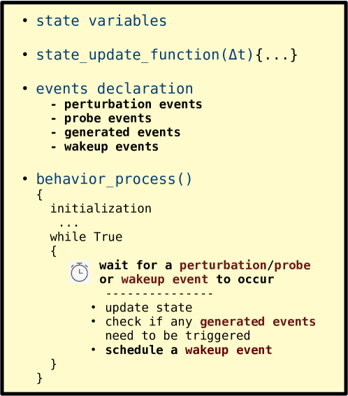
Figure 1: Wrapper for a continuous entity with the events serving as its interface[17]

A continuous entity is characterized by its state variables and a state-update function. The modeler also needs to provide a definition of all events that may be generated by the entity and affect the external world and vice-versa. These events can be classified into four types as follows:

1. Perturbation event: An externally-created event that may affect the state/trajectory of the continuous entity.

2. Probe event: An externally-created event which involves querying the state of the continuous entity and thus necessitates updating its state up-to a given time.

3. Generated event: An event triggered by the continuous entity itself as a consequence of its state update which may affect other entities in the system.

4. Wakeup event: An event scheduled by the continuous entity itself for performing state updates after a fixed time step or for creating generated events whose time of occurrence can be predicted in advance.

The behaviour of the continuous entity is modeled as a discrete-event process. This process is activated whenever a perturbation, probe or a wakeup event for the entity occurs. When activated:

1. The state updates for the entity up-to the current time are computed.

2. If any condition for generating output events is met (for example, the state variable crossed a threshold), the generated events are triggered.

3. The continuous entity schedules a wakeup event for itself after a particular time interval. This time interval is determined based on one of two approaches as follows:

   • (a) Predictive time-stepping: If the current trajectory of the state values in the entity is known, and if all of the output events can be predicted ahead of time based on this trajectory, the wakeup can simply be scheduled at the time the earliest output event is predicted to occur. (This is illustrated via the example of a fluid tank described in Section 3.2.

   • (b) Fixed time-stepping: If the exact time instants of events that will be generated by this entity cannot be predicted ahead of time, the state needs to be updated after regular time intervals that are small enough, by scheduling a wakeup event periodically. The step-size may need to be chosen based on numerical stability requirements. (This is illustrated via the example of a heater entity described in Section 3.1.

At each iteration of the event-stepped algorithm, the simulation time is advanced to the time-stamp of the earliest scheduled event in the global event list. All events scheduled to occur at this time are executed and the processes waiting on this event are automatically triggered (using a mechanism such as callbacks) provided by the discrete-event framework.

It is to be noted that if the system has multiple continuous entities requiring fixed time-stepping, and if the chosen step-sizes of these entities differ, then in this approach, each entity will be woken up periodically as per its own step-size only, unless there is an external event affecting it. This leads to an efficient simulation, where some entities may be updated with a coarse time-step while some may use a finer time-step.

2.2 Implementation

We have implemented the MDCS framework using SimPy[28], a discrete-event simulation library in Python. Processes in SimPy are implemented using Python’s generator functions and can be used to model active components. The processes are managed by an environment class, which performs time advancement in an event-stepped manner using a global event queue. The system to be modeled can be described in Python using a few SimPy constructs and does not require the user to learn a new modeling language. SimPy also supports real-time simulation. However, SimPy is designed for discrete-event simulation and currently offers no features for modeling continuous systems [28]. The events-based interface presented in this paper can be implemented as an abstract wrapper class to allow integration of continuous entities. The modeler needs to create the wrapper class for each unique type of continuous entity describing the aspects summarized in Figure 1. When the simulation of the continuous entity needs to be performed using an external solver (such as Deal II or OpenFOAM), the state update function in the abstract class serves as a wrapper for invoking the state updates via the external continuous solver. Similarly, the continuous solver code needs to be instrumented to detect conditions that must trigger events, and set a flag variable in the wrapper. State or boundary value updates to the continuous entity can be implemented via global shared variables that may be updated by external processes, but are read at each iteration in the continuous solver code. The implementation is straightforward if the simulation and state updates for the continuous entity are also described as Python code. In the example presented in Section 3 the state updates of continuous entities are performed directly by including their description as Python modules.

3 A Modeling Example

We present a modeling example to illustrate the key aspects of the MDCS framework. The system to be modeled consists of discrete-event processes as well as two types of entities that are modeled in the continuous domain. The first type of entity (a fluid tank) has simple, linear state-update equations. Simulation of this entity can be performed using the predicted time-stepping approach. The second entity is a heater with a square-shaped plate which can be heated from two opposite sides. The temperature within the plate varies continuously with time and also across the length and breadth of the plate. The diffusion of heat in the plate is simulated using fixed time-stepping approach, with the time-step size determined by numerical stability requirements. The complete system to be simulated consists of both types of components interacting with each other.

We first describe each of these components and their simulation approaches in detail. We then describe the complete system consisting of the fluid tank and the heater instances interacting with each other as well as with other discrete-event processes. We show how the interactions can be described in the framework, and present detailed simulation results.

3.1 Heater

3.1.1 Description:

The physical system consists of a square-shaped hot-plate with each side $1$m long and made of a composite material. Two opposite edges of this plate can be heated with the help of heating coils. We make the simplifying assumption that the heating coils instantly reach the steady-state high temperature value without any lag when switched on. The remaining two edges of the hot-plate are maintained at a constant lower temperature at all times. After the heating coils are turned on, heat dissipates in the hot-plate and eventually the temperature distribution attains a steady state profile. How quickly the heat dissipates depends on the thermal conductivity, the specific heat capacity and the density of the material of the hot-plate. A physical parameter called as thermal diffusivity ($\alpha$, units m²/s) is often used to describe the resistance offered by any material for heat dissipation. It takes into account the collective effects due to all the material properties mentioned above. We assume the hot-plate to be made of a highly conductive composite material with thermal diffusivity equal to $0.0005$m²/s. When the heater is turned off, the heat starts flowing out via all the four edges. We assume the convective and the radiative losses to be negligible and the entire heating and cooling of the hot-plate takes place only through the boundaries. We measure the temperature of the hot-plate with the help of a temperature probe. The framework allows specifying the location of the probe at any location. We assume the probe to locate at the center of the plate in this example. For this test case, we specify the heater temperature (when turned ON) as $100^{0}$C (HIGH_temp) and the room temperature, which is also the temperature maintained constantly at the other two edges, as $25^{0}$C (LOW_temp). Further, when the heating is switched OFF, all the four boundaries are assumed to be at the uniform temperature equal to LOW_temp. Figure 2 shows a schematic of the hot-plate along with the state-variables and the state-update equations governing the conductive heat transfer.

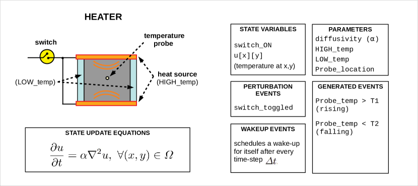
Figure 2: Description of the Heater model

3.1.2 Numerical Simulation:

Let the hot-plate be modeled by a square shaped computational domain $\Omega:=[0,1]\times[0,1]$. Let the temperature in the plate be described by $u(x,y)$, where $(x,y)$ is any physical location. Further, time is denoted by $t$. The thermal diffusivity $\alpha$ is a material-specific property, which depends on the thermal conductivity of the material, its specific heat capacity and its density. The heat conduction through a homogeneous material is described mathematically by the following Partial Differential Equation (PDE).

$$\frac{\partial u}{\partial t}=\alpha\nabla^{2}u,~{}\forall(x,y)\in\Omega$$ (1)

The boundary conditions are as follows. $u(x,0)=u(x,1)=$ Heater temperature: i.e. HIGH_temp (heater ON) or LOW_temp (heater OFF) and $u(0,y)=u(1,y)=$ LOW_temp $\forall$ t.

To solve this equation numerically, we use the Finite Difference Method (FDM). First, the domain $\Omega$ is discretized in a structured, uniform grid with the grid-spacing $h$. Let the number of grid-points in each direction $x$ and $y$ be $N$, i.e. $N^{2}$ in total. Therefore, the location of any grid-point $(i,j)$ is given as $(x_{i},y_{j})=(ih,jh),~{}i,j=0,1,2,...,N-1$ . Similarly, let the time-step for advancing the numerical simulation be $\Delta t$. The temperature at any grid-point $(i,j)$ at time level $k$ is denoted as $u_{i,j}^{k}$. The difference equation corresponding to the governing equation (1) can be written as (derived from Taylor’s series expansion, i.e. standard FDM formulation):

$$\frac{u_{i,j}^{k+1}-u_{i,j}^{k}}{\Delta t}=\alpha\left(\frac{u_{i+1,j}^{k}-2u_{i,j}^{k}+u_{i-1,j}^{k}}{h^{2}}+\frac{u_{i,j+1}^{k}-2u_{i,j}^{k}+u_{i,j+1}^{k}}{h^{2}}\right)$$ (2)

with the Dirichlet boundary conditions given as

$$u_{0,j}^{k}=u_{N-1,j}^{k}=\textnormal{{\tt LOW\_temp}}$$

and

$$u_{i,0}^{k}=u_{i,N-1}^{k}=\textnormal{{\tt HIGH\_temp} (heater {\tt ON}) or {\tt LOW\_temp} (heater {\tt OFF})}$$

Equation (2) can be further simplified as

$$u_{i,j}^{k+1}=\gamma\left({u_{i+1,j}^{k}+u_{i-1,j}^{k}}+{u_{i,j+1}^{k}+u_{i,j+1}^{k}}-{4u_{i,j}^{k}}\right)+u_{i,j}^{k}$$ (3)

where, $\gamma=\alpha\Delta t/h^{2}$. In the beginning of the simulation, the initial conditions $u_{i,j}^{0}=\textnormal{\tt LOW\_temp},\forall i,j$ hold true for the entire domain. Equation (3) is solved iteratively to advance the simulation in time. This time-stepping scheme is also known as the Forward-Euler (FE) explicit timestepping scheme. It is to be noted that, the FE timestepping scheme is only conditionally stable, i.e. the time-step value needs to be ‘small’ enough to yield stable computations. According to the Von-Neumann stability analysis, the time-step value comes out to be $\Delta t\leq h^{2}/(4\alpha)$. i.e. this is the largest value of $\Delta t$ that can be safely used for advancing the solution in time. This in turn also dictates the frequency of wake-up events that needs to be scheduled. An efficient, vectorized implementation of Equation (3) is performed using Numpy, a Python library for scientific computing. Python also makes it convenient to incorporate the numerical implementation of the heater in the discrete event framework.

3.1.3 Interface with the Discrete-Event Simulation Framework

The heater entity is implemented as a Python class. The state variables, parameters and the state-update function (i.e. the numerical solution of the governing PDE given by Equation 1) become the members of this class. The interaction of the heater with the environment happens via the following types of events:

1. Perturbation Events: These are the events which can cause the heating coils to turn on or off. This in turn results in heat transfer into or out of the system affecting the temperature distribution.

2. Probe Events: We can specify the location of the probe on the hot-plate. External components can probe the temperature at this location at the current simulation time. This necessitates the updating the heater state up-to the current time. If time at which the probing is performed is sooner than the next wake-up governed by the time-step $\Delta t$ corresponding to the Forward Euler method, an update at a smaller time-step is performed. Since this doesn’t affect the stability of the numerical method, the update can be safely performed.

3. Generated Events: User can specify a threshold value of temperature (or multiple values) at the probe location. Whenever the rising temperature at the probe location crosses the threshold values, an event (probe-temperature crossed (rising)) is generated. Similarly whenever the falling temperature at the probe location crosses the threshold value, another event (probe-temperature crossed (falling)) is generated. External processes waiting for these events to occur are then automatically notified (using the yield <event> construct of SimPy).

4. Wake-up Events: Since numerical solution of the governing PDE requires an iterative time-stepping scheme, a wake-up event is generated after every time-step which schedules the state-update for the next time-step. The time-step size is governed by the stability requirements of the numerical method. If any other event (probe/perturbation/generated) occurs before the scheduled wake-up takes place, a state-update is scheduled by those events as described earlier. Once those events are executed, the system resumes the wake-up cycle for advancing in time.

3.1.4 Numerical Results

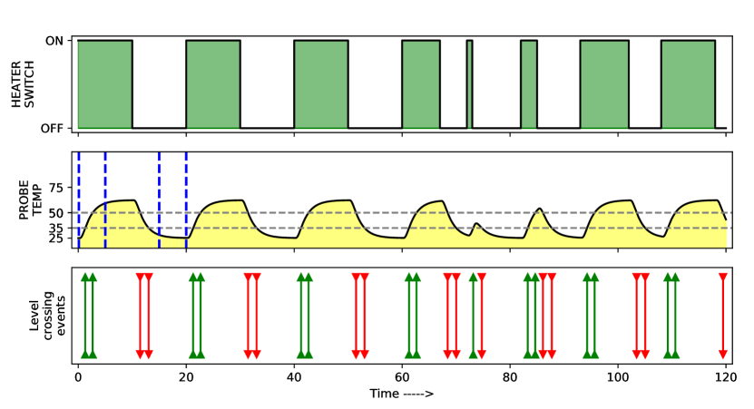
Figure 3: Time evolution of the probe temperature showing events generated during simulation. The level crossing events (rising and falling) are shown with upward and downward arrows respectively. The threshold temperatures were set at $35^{0}$C and $50^{0}$C.

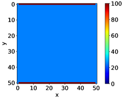
(a) $T=\Delta T$min

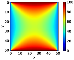
(b) $T=5$min

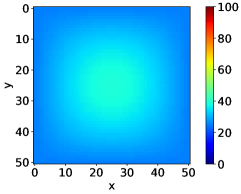
(c) $T=15$min

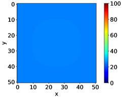
(d) $T=20$min

Figure 4: Temperature profile snapshots at time $T=\Delta t,5,15,20$ mins.

We validate the heater model as follows. A heating and cooling schedule is designed to validate the heater model. The schedule consists of two identical cycles of heating and cooling in the time span of first $50$min, and a random heating and cooling schedule from $T=50$min to $T=120$min. Both cycles till $T=50$min are of identical time duration and consist of a heating process followed by a cooling process. Figure 3 shows a time-series plot of the temperature at the center of the hot-plate (measured by the probe). The framework allows specifying threshold temperature values to schedule Generated Events. In this example, we have set two temperature values, i.e. $u=35^{0}$C and $u=50^{0}$C as shown in the figure. Whenever the rising temperature at the probe location crosses the threshold values, a Generated Event (probe-temperature rising, denoted by green upward pointing arrow) is created. Similarly whenever the falling temperature crosses the threshold values, another generated event (probe-temperature falling, denoted by red downward pointing arrow) is created. These generated events can affect either the discrete event schedule or other continuous systems in the framework. The entire simulation is run through a discrete event scheduler, which schedules a wake-up event for each time step to advance the simulation in time. It can be seen that, the temperature at the center of the hot-plate starts increasing when the heater is turned ON and asymptotically reaches a steady-state value of $62.8^{0}$C. At time $T=12.5$min, the heater is turned OFF and the temperature starts dropping exponentially until it reaches the LOW_temp value of $25^{0}$C. As the heat loss takes place only at the edges, a higher residual temperature remains at the interior parts of the hot-plate for a short time even after the heater is turned OFF. Eventually the heat loss results in a uniform temperature of $25^{0}$C over the entire area of the hot-plate. Figure 4 shows snapshots of the hot-plat at time $\Delta t,5,15$ and $20$ minutes, where, $\Delta t$ is the time after the first time-step is performed. Corresponding time-values are highlighted in 3 with dashed blue lines. It can be clearly seen that, at $\Delta t$ the two opposite edges are at HIGH_temp while the rest of the hot-plate is at LOW_temp. The value of $\Delta t$ is dictated by the stability conditions as stated earlier. At $T=5$min, heat has dissipated inside the domain raising the temperature differentially at different parts. After the heating is turned OFF, a residual high temperature is observed for a short while in the interior parts of the plate, for example as shown in the figure at $T=15$min. This residual temperature returns to LOW_temp as the heat loss takes place through all four boundaries. Sometime before $T=20$min, the temperature over the entire domain asymptotically returns to $25^{0}$C. The cycle repeats after $T=25$min till $T=50$min. After $T=50$min, the heating and cooling schedule is kept random. This is to demonstrate that the heating and cooling can be randomly applied in the ongoing simulation and an a-priori knowledge of the same is not required for running the simulation. This has been made possible due to our approach to time-stepping the simulation via a discrete event scheduler, including for the embedded continuous processes. In the subsequent sections, we demonstrate an example where the heater works along with another continuous simulation entity (water tank) in the discrete event framework, such that both the discrete event framework and the continuous entities can potentially have an effect on each other.

3.2 Fluid Tank

3.2.1 Description:

Consider a fluid tank whose level is to be simulated and monitored continuously with respect to time. The tank has inlet and outlet valves that can be opened and closed based on external triggers. Opening/closing of these valves changes the state trajectory of the tank. The flow rate through the inlet/outlet are assumed to be fixed parameters in the model. They are specified in units of length per-time and defined as maximum change in the fluid level per unit time when the corresponding valve is open. Further, the maximum level at which the tank is considered full, is also a parameter.

The state-update equations for the tank, along with a summary of the state variables and parameters is presented in Figure 5. For this continuous entity, the state-update equation is a simple linear algebraic equation and therefore, an iterative time marching method is not necessary. The state after a given time interval $\Delta t$ can be directly computed from the current state as long as the condition of the inlet/outlet valves do not change. We now describe how this continuous entity interacts with the external processes, and how its simulation can be performed by time-advancement through the discrete-event engine.

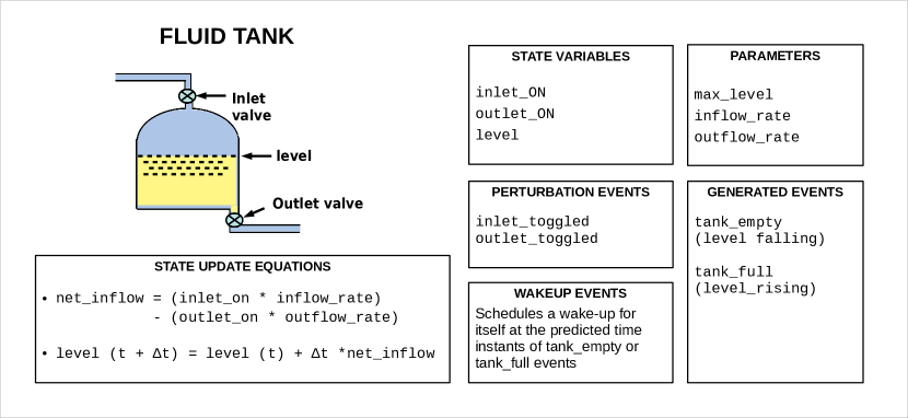
Figure 5: Model of a fluid tank

3.2.2 Discrete-Event Interface and Simulation:

The tank entity can be implemented as a Python class with an interface similar to that in Figure 1. The state variables, parameters and the state-update function become members of this class. The tank interacts with the environment via the following events serving as an interface:

1. Perturbation Events: External events can cause the tank’s inlet or outlet valves to toggle their state, which can change the trajectory of the level.

2. Probe Events: External components can probe the level of the tank at the current simulation time. This necessitates updating the tank state up-to the current time.

3. Generated Events: Whenever the tank level falls, and the tank becomes empty, a tank_empty event is generated and triggered by the tank entity itself. External processes waiting for this event to occur are then automatically notified (using the yield <event> construct of SimPy). Similarly, when the tank level is rising and reaches the maximum value, a tank_full event is generated.

4. Wake-up Events: Owing to the linear state-update equations, the state updates need not be performed periodically at fixed time-steps. Rather they can be performed directly at time-instants of interest. Whenever a state-update is performed, the future time instant at which the tank is expected to become empty (if the level is falling) or full (if the level is rising) is computed, and the entity schedules a wake-up event for itself at this precise time instant. When the wake-up event (or any perturbation/probe/generated events) occur in the tank, the state-update is performed, empty/full events are triggered if the tank has become empty/full at this instant, and the next wake-up event is scheduled, based on the current trajectory.

   If it so happens that tank’s state trajectory changes sometime before the next wake-up event (for instance, due to the toggling of a valve), the state is updated and a new wake-up event is scheduled based on the updated trajectory. The old wake-up event however is not cancelled. It simply causes the tank state to be updated up-to the time instant of the old wake-up event and does not have any side effects on the state.

3.2.3 Validation and Simulation Results:

Figure 6 shows the simulation results obtained for a simple validation exercise involving a single tank instance. Here, an external SimPy process toggles the tank’s inlet and outlet valves after random time intervals. The generated tank_empty and tank_full events are also indicated in the plot.

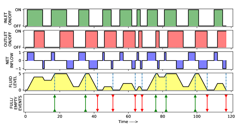
Figure 6: A plot of the time evolution of the tank’s state showing the empty/full events generated during simulation. The inlet/outlet values are toggled after random time intervals

3.3 The System

We now describe the complete system where the fluid tank and heater instances interact with each other and with the environment through the events interface. To illustrate a two-way dependency between the fluid tank and heater instances, we model the following interactions in the system:

1. At the start of simulation, the heater is assumed to be OFF and the temperature of the entire heating plate is set to the LOW_temp value of $25^{0}$C. The fluid tank is assumed to be full. The tank’s inlet and outlet valves are both closed.

2. The heater is turned ON. As soon as the probe temperature crosses a certain threshold (in this case $50^{0}$C), the system can start processing external jobs one-by-one. The arrival of jobs is modeled by a stochastic discrete-event process.

3. Each arriving job has a duration which is random and uniformly distributed between 0.5 to 1 minutes. Also the time interval between arrival of successive jobs is also uniformly distributed between 0.5 to 1 minutes. The tank outlet valve needs to be kept open for the duration of each job. Thus the tank gradually empties as successive jobs are processed.

4. As soon as the tank becomes empty, the heater is turned OFF, and the tank refill process is initiated. The tank inlet valve is opened and the outlet valve is closed. The tank gradually becomes full again.

5. As soon as the tank becomes full, the entire loop is repeated, starting from step 2.

To implement these interactions, an additional Python class (Controller) is created. The behavior of the controller can be described in a straightforward manner as a SimPy process. Listing 1 is an excerpt from the controller’s behavioral loop described above. The code listing serves to highlight the ease with which complex interactions between continuous and discrete-event entities can be described by the modeler. Figure 7 presents simulation results generated for this system. The causality of events is indicated in the figure by dashed arrows. The simulation also produces a detailed event log.

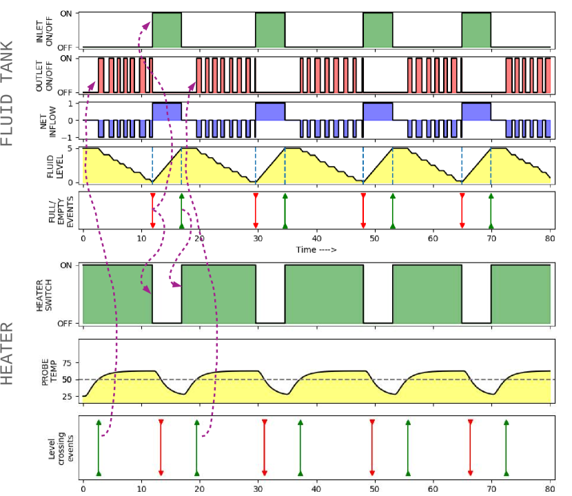
Figure 7: Simulation results for a system containing interacting tank and heater instances. The causality of events is indicated by dashed arrows.

⬇

1# Python code excerpt describing the control loop

2# note: env is an instance of SimPy’s environment object

3

4class Controller():

5 # initialization, and other member functions

6 # .....

7

8 def controller_behavior(self,env):

9

10 # initially the tank is full and its valves are closed.

11 tank.level=tank.max_level

12 tank.inlet_ON=False

13 tank.outlet_ON=False

14 # initially the heater is off. check this.

15 assert(not heater.is_heater_ON())

16

17 while(True):

18

19 # turn ON the heater

20 heater.turn_ON_heater_switch()

21 # wait until the probe temperature goes

22 # above a set threshold.

23 if(heater.probe_temp() < 50):

24 yield heater.threshold_crossed_rising_event

25

26 # now, start processing jobs by periodically

27 # toggling the tank outlet valves. Do this until

28 # the tank level falls below a threshold.

29

30 while(not tank.is_empty()):

31 # turn ON the tank valve

32 tank.toggle_outlet_valve()

33 job_duration = random.uniform(0.5, 1)

34 job_done = env.timeout(job_duration)

35 tank_empty = tank.empty_event

36

37 # wait until the job is done or the tank becomes empty

38 what_occured = yield (job_done | tank_empty)

39

40 if job_done in what_occured:

41 # wait for some time and then repeat with next job

42 tank.turn_OFF_outlet_valve()

43 idle_duration = random.uniform(0.5, 1)

44 yield env.timeout(idle_duration)

45 else:

46 # tank became empty.

47 break

48 # tank became empty. Now turn OFF the heater,

49 # and start the tank refilling process.

50 # then, wait until the tank becomes full again.

51 heater.turn_OFF_heater_switch()

52 tank.turn_OFF_outlet_valve()

53 tank.turn_ON_inlet_valve()

54 yield tank.full_event

55

56 # now the tank has become full.

57 # turn off the tank valves.

58 tank.turn_OFF_inlet_valve()

59 tank.turn_OFF_outlet_valve()

60 # done. repeat the loop.

Listing 1: Python excerpt for implementing the system control loop described in Section 3.3

4 An Improved Scheme for Time Advancement

As discussed in Section 2, time advancement can be performed using either a predictive time-stepping approach, or using fixed time-steps when the governing equations of the continuous entity require iterative state updates. One issue with the fixed time-step approach is that if the time step size for the continuous simulation is very small relative to the typical time between events in the rest of the system, the cost of adding a wakeup event to the global event list after every time-step can be prohibitive. To address this, the following modification can be used:

At each iteration ($K$) of the event-stepped algorithm, the tentative time-step ($\Delta_{K}$) is taken to be the difference between the scheduled time of the next event in the global event list ($t_{\textrm{next\_event}}$) and the simulation time for the current iteration($t_{K}$).

$$\Delta_{K}=t_{\textrm{next\_event}}-t_{\textrm{K}}$$

Each continuous entity is then asked to peek-ahead in time by a total period of $\Delta_{K}$ by executing its state-update equations. This can be done either using a single step of size $\Delta_{K}$ or by dividing this period into finer time-steps as as dictated by the time marching scheme. The computation of state updates for multiple continuous entities can potentially be executed in parallel. If no output events of interest are predicted to be generated by any of the continuous entities in this period, the time can be advanced by $\Delta_{K}$ and the computed state-updates in each of the continuous entities can be applied before proceeding to the next iteration. However, if it is found that for a continuous entity $i$, an event of interest is generated at time $t_{i}<t_{\textrm{next\_event}}$, then it may be possible that this event could affect the state or trajectories of the other entities in the system. Thus the actual time-step taken must be the one that advances time to the earliest predicted event across all of the continuous entities. That is, the simulation time should be advanced to $t_{K+1}=\textrm{min}_{i}(t_{i})$ in the next iteration.

The earliest event predicted to occur at time $t_{K+1}$ can then be inserted into the global event-list, so that its effect on other entities can be propagated as usual in a discrete-event framework, and the state updates in all of the continuous entities computed up to time $t_{K+1}$ can be applied before advancing simulation time to $t_{K+1}$. A further optimization is to adaptively adjust the tentative time step $\Delta_{K}$ for improved performance. Implementing this requires the continuous simulation framework to support a peek-ahead or roll-back feature.

A second approach is to use meta-modeling (in the form of regression-based models, neural networks with supervised learning, or physics-informed neural networks) for predicting the time instants of generated events in advance. In fact, detailed models of continuous processes can often be replaced by reduced order surrogate models when accuracy needs to be traded for evaluation speed. In such models, the time instants of generated events can be predicted ahead of time, and the predictive time-stepping approach can be used for efficient simulation. Exploring the use of these approaches for building digital twins is a promising direction.

5 Future Work and Conclusions

In this paper we presented a Python based Mixed Discrete-Continuous Simulation (MDCS) framework specifically targeted for Digital Twins applications. The framework is based on Python’s SimPy library and uses its event-stepped algorithm for coordinating the time advancement. We presented a detailed example of interacting continuous entities simulated using this framework. The design aspects of the framework and the simulation approach make it well-suited for digital twin applications for the following reasons:

• The event-stepped approach can result in a more efficient simulation for scenarios where only a few kinds of events affect the trajectory of continuous entities in the system.

• In this approach, it is possible for different continuous entities in the system to use different continuous solvers and internal time step-size values.

• The loose coupling between the continuous entities presents opportunities for executing their behavior in parallel within a single time-step for real-time simulation.

• For modeling entities where a high level of accuracy may not be necessary, coarse surrogate models can be used to predict the trajectory and time of generated events and schedule a wakeup ahead of time.

• Sensor value updates from the real system can be easily incorporated into the simulation as perturbation events affecting the state.

Future improvements to the framework are planned along the following directions:

1. Integration with existing continuous simulation frameworks

   For fast simulation of continuous processes, integration with established continuous simulation frameworks is necessary. This requires building wrappers for invoking state update functions of continuous solvers such as OpenFOAM. We also plan to integrate Dolfin [23], a Python based finite-element library for multiphysics modeling and simulation.

2. Incorporating analytics

   For Digital Twin applications, analytics modules need to be incorporated into the framework for parameter extraction from sensor data, prediction, optimization and for building surrogate models in run-time.

3. Acceleration for real-time simulations

   The requirement for real-time simulation creates a need for simulation acceleration that is possible using hardware platforms such as GPGPUs, FPGAs or parallel execution on multi-core systems. It is possible to explore architectures that can take advantage of these technologies for simulations.

4. Support for sensing and control

   Sensing and control are integral aspects of a Digital Twin. Features that support these aspects need to be explored and integrated into the framework.

References

- [1] Agalianos, K., Ponis, S.T., Aretoulaki, E., Plakas, G., Efthymiou, O.: Discrete Event Simulation and Digital Twins: Review and Challenges for Logistics. Procedia Manufacturing 51(2019), 1636–1641 (2020). https://doi.org/10.1016/j.promfg.2020.10.228, https://doi.org/10.1016/j.promfg.2020.10.228
- [2] Aimone, J., Parekh, O., Severa, W.: Neural computing for scientific computing applications. In: ACM International Conference Proceeding Series. vol. 2017-July (2017). https://doi.org/10.1145/3183584.3183618
- [3] Aversano, G., Ferrarotti, M., Parente, A.: Digital Twin of a Combustion Furnace Operating in Flameless Conditions: Reduced-Order Model Development from CFD Simulations. Proceedings of the Combustion Institute 000, 1–9 (2020). https://doi.org/10.1016/j.proci.2020.06.045, https://doi.org/10.1016/j.proci.2020.06.045
- [4] Bangerth, W., Davydov, D., Heister, T., Heltai, L., Kanschat, G., Kronbichler, M., Maier, M., Turcksin, B., Wells, D.: The deal.II Library, Version 8.4. J. Numer. Math. 24, 135–141 (2016). https://doi.org/10.1515/jnma-2016-1045
- [5] Bechard, V., Cote, N.: Simulation of Mixed Discrete and Continuous Systems: An Iron Ore Terminal Example. In: 2013 Winter Simulations Conference (WSC). pp. 1167–1178 (2013). https://doi.org/10.1109/WSC.2013.6721505
- [6] Brunton, S.L., Noack, B.R., Koumoutsakos, P.: Machine Learning for Fluid Mechanics. Annual Review of Fluid Mechanics 52, 477–508 (2020). https://doi.org/10.1146/annurev-fluid-010719-060214
- [7] Cellier, F.E., Kofman, E.: Continuous System Simulation. Springer-Verlag, US (2006)
- [8] Chinesta, F., Ladeveze, P., Cueto, E.: A Short Review on Model Order Reduction Based on Proper Generalized Decomposition. Archives of computational methods in engineering 18, 395–404 (2011). https://doi.org/10.1007/s11831-011-9064-7
- [9] Dagkakis, G., Heavey, C.: A Review of Open Source Discrete Event Simulation Software for Operations Research. Journal of Simulation 10(3), 193–206 (2016). https://doi.org/10.1057/jos.2015.9, https://doi.org/10.1057/jos.2015.9
- [10] Damiron, C., Nastasi, A.: Discrete Rate Simulation Using Linear Programming. In: Winter Simulation Conference Proceedings. pp. 740–749 (2008). https://doi.org/10.1109/WSC.2008.4736136
- [11] Eldabi, T., Tako, A.A., Bell, D., Tolk, A.: Tutorial on Means of Hybrid Simulation. Proceedings of the 2019 Winter Simulation Conference pp. 273–284 (2019)
- [12] Feng, L.: Review of Model Order Reduction Methods for Numerical Simulation of Nonlinear Circuits. Applied Mathematics and Computation 167, 576–591 (2005). https://doi.org/10.1016/j.amc.2003.10.066
- [13] Fritzson, P., Pop, A., Abdelhak, K., Ashgar, A., Bachmann, B., Braun, W., Bouskela, D., Braun, R., Buffoni, L., Casella, F., Castro, R., Franke, R., Fritzson, D., Gebremedhin, M., Heuermann, A., Lie, B., Mengist, A., Mikelsons, L., Moudgalya, K., Ochel, L., Palanisamy, A., Ruge, V., Schamai, W., Sjölund, M., Thiele, B., Tinnerholm, J., Östlund, P.: The OpenModelica Integrated Environment for Modeling, Simulation, and Model-Based Development. Modeling, Identification and Control 41(4), 241–295 (2020). https://doi.org/10.4173/mic.2020.4.1
- [14] Giambiasi, N., Escude, B., Ghosh, S.: GDEVS: A Generalized Discrete Event Specification for Accurate Modeling of Dynamic Systems. Proceedings - 5th International Symposium on Autonomous Decentralized Systems, ISADS 2001 pp. 464–469 (2001). https://doi.org/10.1109/ISADS.2001.917452
- [15] Hill, R.: Discrete-Event Simulation: A First Course. Journal of Simulation 1(2), 147–148 (2007). https://doi.org/10.1057/palgrave.jos.4250012
- [16] Huda, A.M., Chung, C.A.: Simulation modeling and analysis issues for high-speed combined continuous and discrete food industry manufacturing processes. Computers and Industrial Engineering 43(3), 473–483 (2002). https://doi.org/https://doi.org/10.1016/S0360-8352(02)00120-1, https://www.sciencedirect.com/science/article/pii/S0360835202001201
- [17] Karanjkar, N., Joshi, S.M.: Mixed Discrete-Continuous Simulation for Digital Twins. In: Proceedings of the 11th International Conference on Simulation and Modeling Methodologies, Technologies and Applications, SIMULTECH 2021, Online Streaming, July 7-9, 2021. pp. 422–429. SCITEPRESS (2021). https://doi.org/10.5220/0010580804220429, https://doi.org/10.5220/0010580804220429
- [18] Karniadakis, G.E., Kevrekidis, I.G., Lu, L., Perdikaris, P., Wang, S., Yang, L.: Physics-informed machine learning. Nature Reviews Physics 3(6), 422–440 (2021). https://doi.org/10.1038/s42254-021-00314-5
- [19] Klingener, J.F.: Combined Discrete-Continuous Simulation Models in Promodel for Windows. In: Winter Simulation Conference Proceedings. pp. 445–450 (1995)
- [20] Klingener, J.F.: Programming Combined Discrete-Continuous Simulation Models for Performance. In: Winter Simulation Conference Proceedings. pp. 833–839 (1996). https://doi.org/10.1145/256562.256824
- [21] Kofman, E.: Discrete Event Simulation of Hybrid Systems. SIAM Journal on Scientific Computing 25(5), 1771–1797 (2004). https://doi.org/10.1137/S1064827502418379
- [22] LeVeque, R.J.: Numerical Methods for Conservation Laws. Birkhauser-Verlag, Basel (1990)
- [23] Logg, A., Wells, G.N.: DOLFIN: Automated Finite Element Computing. ACM Trans. Math. Softw. 37(2) (Apr 2010). https://doi.org/10.1145/1731022.1731030, https://doi.org/10.1145/1731022.1731030
- [24] Molinaro, R., Singh, J.S., Catsoulis, S., Narayanan, C., Lakehal, D.: Embedding Data Analytics and CFD into the Digital Twin Concept. Computers and Fluids 214, 104759 (2021). https://doi.org/10.1016/j.compfluid.2020.104759, https://doi.org/10.1016/j.compfluid.2020.104759
- [25] Nutaro, J., Kuruganti, P.T., Protopopescu, V., Shankar, M.: The Split System Approach to Managing Time in Simulations of Hybrid Systems Having Continuous and Discrete Event Components. Simulation 88(3), 281–298 (2012). https://doi.org/10.1177/0037549711401000
- [26] Shao, G., Jain, S., Laroque, C., Lee, L.H., Lendermann, P., Rose, O.: Digital Twin for Smart Manufacturing: The Simulation Aspect. Proceedings - Winter Simulation Conference 2019-Decem(Bolton 2016), 2085–2098 (2019). https://doi.org/10.1109/WSC40007.2019.9004659
- [27] Simpson, T.W., Peplinski, J.D., Koch, P.N., Allen, J.K.: Metamodels for Computer-based Engineering Design: Survey and Recommendations. Engineering with Computers 17, 129–150 (2001)
- [28] SimPy-Team: Simpy: Discrete-event simulation for python {Online https://simpy.readthedocs.io/en/latest/} (2020)
- [29] Weller, H.G., Tabor, G., Jasak, H., Fureby, C.: A Tensorial Approach to Computational Continuum Mechanics Using Object-Oriented Techniques. Computers in Physics 12(6), 620–631 (1998). https://doi.org/10.1063/1.168744, https://aip.scitation.org/doi/abs/10.1063/1.168744
- [30] Zeigler, B.P.: Devs Representation of Dynamical Systems: Event-Based Intelligent Control. Proceedings of the IEEE 77(1), 72–80 (1989). https://doi.org/10.1109/5.21071