Abstract: For a class of uncertain systems with large-error sensing, the low-order stable signal corrector and observer are presented for signal correction and uncertainty estimation according to completely decoupling estimation. The signal corrector can reject the large error in global position sensing, and system uncertainty can be estimated by the observer, even the existence of stochastic non-Gaussian noise. The corrector and observer are applied to a UAV navigation and control for large-error corrections in position/attitude angle and the uncertainties estimation in the UAV flight dynamics. The control laws are designed according to the correction-estimation results. Finally, experiments demonstrate the effectiveness of the proposed method.

Keywords: Large-error sensing, uncertainty, signal corrector, decoupling estimation

1 Introduction

Usually UAV flight needs information of position, attitude and dynamic model. Global position plays very important roles for large-range navigation and control [1,2]. Meanwhile, The uncertainties exist in UAV flight dynamics: aerodynamic disturbance, unmodelled dynamics and parametric uncertainties are inevitable. These uncertainties bring serious challenges for control system design.

GPS (Global positioning system) can provide position information with accuracy of several meters or even tens of meters [3,4]. Also, the adverse circumstances may contaminate signals from GPS [4]. Velocity is also necessary for UAV navigation and control. GPS can measure device velocity with two different accuracies: 1) large-error velocity by the difference method with accuracy of a meter per second due to GPS position accuracy and noise effect; 2) precise velocity by Doppler shift measurement with accuracy of a few centimeters even millimeters per second [5,6]. Alternatively, accurate velocity of device can be measured by a Doppler Radar sensor [7]. Except for sensing, velocity can be estimated from position using robust observers [8-13]. However, the relatively accurate measurements of position are required.

Without position and velocity sensing, INS (Inertial navigation system) can estimate them through integrations from acceleration measurement. However, even small measurement error or very weak non-Gaussian noise in acceleration through integrations can cause velocity and position to drift over time. The observer-based INS methods were used to estimate unknown variables in navigation [14,15]. However, position signals are limited to be local and bounded, but not global.

For attitude information, an IMU (Inertial Measurement Unit) can determine the attitude angles from the measured angular rates through integration, and angle drifts happen. Meanwhile, the outputs of the accelerometers and the magnetometer in IMU can determine the large-error pitch, roll and yaw angles [16].

In order to reduce large errors in position/attitude angle, KF (Kalman filter) or EKF (Extended Kalman filter) is adopted for signals integration/fusion to restrict the defects of individual measurements [17-19]. Thus, the accuracy of system outputs is improved. However, the noise should be assumed Gaussian distributed, and the estimate error is required to be uncorrelated to the process noise covariance. Because the real noise is stochastic non-Gaussian distributed, drifts in position and attitude are inevitable. Moreover, the existence of system uncertainties limits the KF applications. The uncertainties or disturbances in system can be estimated by the extended state observers [8,11,20-22]. However, the accurate position measurements are required as these observer inputs.

In this paper, a class of uncertain systems with large error in position measurement are considered. As an example, the relevant problems in UAV navigation and control are also considered. According to the relations between position, velocity and uncertainty in system, as well as the large error in position sensing and the relatively accurate measurement in velocity, the position correction and uncertainty estimation are completely decoupled. The independent signal corrector and uncertainty observer are presented according to finite-time stability [23,24] and the complete decoupling. In spite of the existence of stochastic non-Gaussian noise, the stable signal correct can reject the large error in position sensing, and the observer can estimate the system uncertainty. Both corrector and observer are the low-order systems, their system parameters are regulated easily, and oscillations can be avoided. Frequency analysis is used to explain the robustness of the corrector and observer. The signal corrector and uncertainty observer are applied to an experiment on a quadrotor UAV navigation and control, and the performance is compared to the traditional KF-based navigation [25]. In the experiment, the following adverse conditions are considered: large-error measurements in GPS position/IMU attitude angles, uncertainties in position/attitude dynamics, and existence of stochastic non-Gaussian noise. The signal correctors are adopted to correct the large errors in GPS position/IMU attitude angles, and the observers are used to estimate the uncertainties in the UAV dynamics. Finally, the control laws based on the correction and estimation are formed to stabilize the UAV flight.

2 Problem description

The technical problems considered in this paper for a class of uncertain systems with large-error measurement include:

1) large error in position measurement; 2) existence of system uncertainty; 3) overshoot/oscillations existence and difficult parameters selection in high-order estimate systems.

2.1 Correction of large error in position and estimation of uncertainty in position dynamics

Measurement conditions: GPS provides the large-error position of device, and the relatively accurate velocity can be determined by GPS with Doppler shift measurement or by a Doppler Radar sensor. Also, the uncertainties/disturbances exist in system dynamics. Under these conditions, we have:

Question 1: How to correct the error in position and to estimate uncertainty in position dynamics in spite of existence of non-Gaussian noise and large-error position measurement?

2.2 Correction of large error in attitude angle and estimation of uncertainty in attitude dynamics

Measurement conditions: The gyroscopes in IMU provide the direct measurement of relatively accurate angular rate. The large-error attitude angles can be determined by the outputs of the accelerometer and magnetometer in IMU.

Question 2: How to correct large error in attitude angle and to estimate uncertainty in attitude dynamics in spite of existence of non-Gaussian noise and large-error attitude angle measurement?

2.3 Difficult parameters selection and oscillations existence for high-order estimation system

For multivariate estimation/correction, a high-order observer can be used. However, many system parameters need to be adjusted cooperatively, and oscillations are prone to occur. The oscillations can amplify the noise in the estimation outputs. Therefore, we hope the decoupling low-order estimate systems can be designed to overcome these issues instead of a single high-order observer.

3 General form of decoupling corrector and observer for uncertain systems with large error sensing

3.1 Uncertain system with large-error measurement

The following uncertain system has a minimum number of states and inputs, but it retains the features that is considered for many applications:

$$\dot{x}_{1} = x_{2}$$

$$\dot{x}_{2} = h(t)+\sigma(t)$$

$$y_{o1} = x_{1}+d(t)+n_{1}(t)$$

$$y_{o2} = x_{2}+n_{2}(t)$$ (1)

where, $x_{1}$ and $x_{2}$ are the states; $h(t)$ $\in\Re$ is the known function including the controller and the other known terms; $\sigma(t)\in\Re$ is the system uncertainty; $y_{o1}$ and $y_{o2}$ are the sensing outputs; $d(t)$ is the unknown bounded large error in measurement, and $\sup_{t\in[0,\infty)}\left|d(t)\right|\leq L_{d}<+\infty$; $n_{1}(t)$ and $n_{2}(t)$ are the measurement noise. The missions include: error correction in $y_{o1}$; estimation of $\sigma(t)$.

3.2 System extension

Assumption 3.1: Suppose uncertainty $\sigma(t)$ in system (1) satisfies

$$\dot{\sigma}(t)=c_{\sigma}(t)$$ (2)

where, $c_{\sigma}(t)$ is unknown and bounded, and $\sup_{t\in[0,\infty)}\left|c_{\sigma}(t)\right|\leq L_{\sigma}<+\infty$. Actually, this assumption holds for many applications, e.g., crosswind dynamics.

In system (1), in order to estimate the uncertainty $\sigma(t)$, we define it as a new variable, i.e., $x_{3}=\sigma(t)$. Therefore, $\dot{x}_{3}=\dot{\sigma}(t)=c_{\sigma}(t)$ holds. Then, second-order system (1) is extended equivalently into a third-order system, i.e.,

$$\dot{x}_{1} = x_{2}$$

$$\dot{x}_{2} = x_{3}+h(t)$$

$$\dot{x}_{3} = c_{\sigma}(t)$$

$$y_{o1} = x_{1}+d(t)+n_{1}(t)$$

$$y_{o2} = x_{2}+n_{2}(t)$$ (3)

3.3 System decoupling according to the accurate measurement

The estimations of $x_{1}$ and $x_{3}$ are in the opposite directions from the relatively accurate measurement $y_{o2}$. Then, system (3) can be decoupled into the following two systems:

1) the unobservable (from $y_{o2}$) system

$$\dot{x}_{1} = x_{2}$$

$$y_{o1} = x_{1}+d(t)+n_{1}(t)$$

$$y_{o2} = x_{2}+n_{2}(t)$$ (4)

2) and the observable system

$$\dot{x}_{2} = x_{3}+h(t)$$

$$\dot{x}_{3} = c_{\sigma}(t)$$

$$y_{o2} = x_{2}+n_{2}(t)$$ (5)

3.4 General form of completely decoupling correction and estimation

We give the following assumptions before the correction and estimation systems are constructed.

Assumption 3.2: Suppose the origin is the finite-time-stable equilibrium of system

$$\dot{z}_{1} = z_{2}$$

$$\dot{z}_{2} = f_{c}(z_{1},k\cdot z_{2})$$ (6)

where, $f_{c}()$ is continuous and $f_{c}(0,0)=0$, and $k>1$.

Assumption 3.3: For (6), there exist $\rho\in(0,1]$ and a nonnegative constant $a$ a such that

$$\left|f_{c}(\tilde{z}_{1},k\cdot z_{2})-f_{c}(\bar{z}_{1},k\cdot z_{2})\right|\leq a\left|\tilde{z}_{1}-\bar{z}_{1}\right|^{\rho}$$ (7)

where, $\tilde{z}_{1},\bar{z}_{1}\in\Re$.

Remark 3.1: There are many types of functions satisfying this assumption. For example , one such function is $\left|\tilde{x}^{\rho}-\overline{x}^{\rho}\right|\leq 2^{1-\rho}\left|\tilde{x}-\overline{x}\right|^{\rho},\rho\in\left(0,1\right]$.

Assumption 3.4: Suppose the origin is the finite-time-stable equilibrium of system

$$\dot{z}_{3} = z_{4}+f_{o1}(z_{3})$$

$$\dot{z}_{4} = f_{o2}(z_{3})$$ (8)

where, $f_{o1}()$ and $f_{o2}()$ are continuous, and $f_{o1}(0)=0$ and $f_{o2}(0)=0$.

Theorem 3.1 (General form of decoupling signal corrector and uncertainty observer):

System (1) is considered, and Assumptions 3.1$\sim$3.4 hold. In order to correct large error in measurement $y_{o1}$ and to estimate uncertainty $\sigma(t)$ (i.e., $x_{3}$), the completely decoupling second-order corrector and observer are designed, respectively, as follows:

1) Signal corrector

$$\dot{\widehat{x}}_{1} = \widehat{x}_{2}$$

$$\varepsilon_{c}^{3}\dot{\widehat{x}}_{2} = f_{c}(\varepsilon_{c}(\widehat{x}_{1}-y_{o1}),\widehat{x}_{2}-y_{o2})$$ (9)

where, $\varepsilon_{c}\in\left(0,1\right)$; and

2) Uncertainty observer

$$\varepsilon_{o}\dot{\widehat{x}}_{3} = \varepsilon_{o}\widehat{x}_{4}+f_{o1}(\widehat{x}_{3}-y_{o2})+\varepsilon_{o}h(t)$$

$$\varepsilon_{o}^{2}\dot{\widehat{x}}_{4} = f_{o2}(\widehat{x}_{3}-y_{o2})$$ (10)

where, $\varepsilon_{o}\in\left(0,1\right)$. Then, there exist $\gamma_{c}>\frac{3}{\rho}$, $\gamma_{o}>1$ and $t_{s}>0$, such that, for $t\geq t_{s}$,

$$\widehat{x}_{1}-x_{1} = O(\varepsilon_{c}^{\rho\gamma_{c}-1})\text{; }\widehat{x}_{2}-x_{2}=O(\varepsilon_{c}^{\rho\gamma_{c}-2})\text{;}$$

$$\widehat{x}_{3}-x_{2} = O(\varepsilon_{c}^{2\gamma_{o}})\text{; }\widehat{x}_{4}-\sigma(t)=O(\varepsilon_{c}^{2\gamma_{o}-1})$$ (11)

where, $O(\varepsilon_{c}^{\rho\gamma_{c}-1})$ means that the error between $\widehat{x}_{1}$ and $x_{1}$ is of order $O(\varepsilon_{c}^{\rho\gamma_{c}-1})$ [26]. The proof of Theorem 3.1 is presented in Appendix.

Remark 3.2: In the signal corrector (9), the input signals include the measurements $y_{o1}$ and $y_{o2}$, and the states $\widehat{x}_{1}$and $\widehat{x}_{2}$ estimate the system states $x_{1}$ and $x_{2}$, respectively. Importantly, the large error $d(t)$ in measurement $y_{o1}$ is rejected. In the observer (10), the input signal is the measurement $y_{o2}$, and $\widehat{x}_{3}$ and $\widehat{x}_{4}$ estimate $x_{2}$ and uncertainty $\sigma(t)$, respectively. Two independent low-order estimate systems are designed to correct large error in measurement and to estimate the uncertainty, and the completely decoupling estimations are implemented.

4 Implementation of completely decoupling corrector and observer for uncertain systems

In the following, we implement: For a class of uncertain systems with large-error sensing, the completely decoupling low-order corrector and observer are designed to implement signal correction and uncertainty estimation, respectively.

4.1 Design of decoupling low-order corrector and observer for uncertain system with large-error sensing

Theorem 4.1: The following uncertain system is considered:

$$\dot{x}_{1} = x_{2}$$

$$\dot{x}_{2} = h(t)+\sigma(t)$$

$$y_{o1} = x_{1}+d(t)+n_{1}(t)$$

$$y_{o2} = x_{2}+n_{2}(t)$$ (12)

where, $x_{1}$ and $x_{2}$ are the states; $h(t)$ $\in\Re$ is the known function including the controller; $\sigma(t)\in\Re$ is the system uncertainty, $\dot{\sigma}(t)=c_{\sigma}(t)$, and $c_{\sigma}(t)$ is bounded with $\sup_{t\in[0,\infty)}\left|c_{\sigma}(t)\right|\leq L_{\sigma}<+\infty$; $y_{o1}$ and $y_{o2}$ are the measurement outputs; $d(t)$ is the unknown large error in measurement $y_{o1}$, and $\sup_{t\in[0,\infty)}\left|d(t)\right|\leq L_{d}<+\infty$; $n_{1}(t)$ and $n_{2}(t)$ are the measurement noise. In order to correct large error in measurement $y_{o1}$ and to estimate uncertainty $\sigma(t)$, the completely decoupling second-order corrector and observer are designed, respectively, as follows:

1) Signal corrector

$$\dot{\widehat{x}}_{1} = \widehat{x}_{2}$$

$$\varepsilon_{c}^{3}\dot{\widehat{x}}_{2} = -k_{1}\left|\varepsilon_{c}(\widehat{x}_{1}-y_{o1})\right|^{\frac{\alpha_{c}}{2-\alpha_{c}}}\text{sign}\left(\widehat{x}_{1}-y_{o1}\right)-k_{2}\left|\widehat{x}_{2}-y_{o2}\right|^{\alpha_{c}}\text{sign}\left(\widehat{x}_{2}-y_{o2}\right)$$ (13)

where, $k_{1}>0$, $k_{2}>0$, $\alpha_{c}\in(0,1)$, and time-scale parameter $\varepsilon_{c}\in\left(0,1\right)$; and

2) Uncertainty observer

$$\varepsilon_{o}\dot{\widehat{x}}_{3} = \varepsilon_{o}\widehat{x}_{4}-k_{4}\left|\widehat{x}_{3}-y_{o2}\right|^{\frac{\alpha_{o}+1}{2}}\text{sign}\left(\widehat{x}_{3}-y_{o2}\right)+\varepsilon_{o}h\left(t\right)$$

$$\varepsilon_{o}^{2}\dot{\widehat{x}}_{4} = -k_{3}\left|\widehat{x}_{3}-y_{o2}\right|^{\alpha_{o}}\text{sign}\left(\widehat{x}_{3}-y_{o2}\right)$$ (14)

where, $k_{3}>0$, $k_{4}>0$, $\alpha_{o}\in(0,1)$, and time-scale parameter $\varepsilon_{o}\in\left(0,1\right)$. Then, there exist $\gamma_{c}>\frac{6-3\alpha_{c}}{\alpha_{c}}$, $\gamma_{o}>1$ and $t_{s}>0$, such that, for $t\geq t_{s}$,

$$\widehat{x}_{1}-x_{1} = O(\varepsilon_{c}^{\frac{\alpha_{c}}{2-\alpha_{c}}\gamma_{c}-1})\text{; }\widehat{x}_{2}-x_{2}=O(\varepsilon_{c}^{\frac{\alpha_{c}}{2-\alpha_{c}}\gamma_{c}-2})\text{;}$$

$$\widehat{x}_{3}-x_{2} = O(\varepsilon_{c}^{2\gamma_{o}})\text{; }\widehat{x}_{4}-\sigma(t)=O(\varepsilon_{c}^{2\gamma_{o}-1})$$ (15)

where, $O(\varepsilon_{c}^{\frac{\alpha_{c}}{2-\alpha_{c}}\gamma_{c}-1})$ means that the error between $\widehat{x}_{1}$ and $x_{1}$ is of order $O(\varepsilon_{c}^{\frac{\alpha_{c}}{2-\alpha_{c}}\gamma_{c}-1})$. The proof of Theorem 4.1 is presented in Appendix.

4.2 Analysis of stability and robustness

Here, the describing function method is used to analyze the nonlinear behaviors of the corrector and observer. Although it is an approximation method, it inherits the desirable properties from the frequency response method for nonlinear systems. We will find that the corrector and observer lead to perform accurate estimation and strong rejection of noise under the condition of the bounded estimate gains.

In signal corrector (13) and uncertainty observer (14), for the nonlinear function $\left|\ast\right|^{\alpha_{i}}sign\left(\ast\right)$, by selecting $\ast=A_{i}\sin(\omega t)$, its describing function can be expressed by $N_{i}(A_{i})=\frac{\Omega(\alpha_{i})}{A_{i}^{1-\alpha_{i}}}$, where, $\Omega(\alpha_{i})=\frac{2}{\pi}\int_{0}^{\pi}\left|\sin(\omega\tau)\right|^{\alpha_{i}+1}d\omega\tau$, and $\Omega(\alpha_{i})\in\left[1,\frac{4}{\pi}\right)$ when $\alpha_{i}\in\left(0,1\right]$. Therefore, the approximations of signal corrector (13) and uncertainty observer (14) through the describing function method are given, respectively, by

$$\dot{\widehat{x}}_{1} = \widehat{x}_{2}$$

$$\dot{\widehat{x}}_{2} = -\frac{k_{1}\Omega(\frac{\alpha_{c}}{2-\alpha_{c}})}{\varepsilon_{c}^{\frac{6-3\alpha_{c}}{2-\alpha_{c}}}A_{c1}^{\frac{2-2\alpha_{c}}{2-\alpha_{c}}}}\left(\widehat{x}_{1}-y_{o1}\right)-\frac{k_{2}\Omega(\alpha_{c})}{\varepsilon_{c}^{3}A_{c2}^{1-\alpha_{c}}}\left(\widehat{x}_{2}-y_{o2}\right)$$

and

$$\dot{\widehat{x}}_{3} = \widehat{x}_{4}-\frac{k_{4}\Omega(\frac{1+\alpha_{o}}{2})}{\varepsilon_{o}A_{o}^{\frac{1-\alpha_{o}}{2}}}\left(\widehat{x}_{3}-y_{o2}\right)+h\left(t\right)$$

$$\dot{\widehat{x}}_{4} = -\frac{k_{3}\Omega(\alpha_{o})}{\varepsilon_{o}^{2}A_{o}^{1-\alpha_{o}}}\left(\widehat{x}_{3}-y_{o2}\right)$$ (17)

Then, we get the natural frequency of the corrector by

$$\omega_{c}=\frac{\sqrt{\Omega(\frac{\alpha_{c}}{2-\alpha_{c}})k_{1}}}{\varepsilon_{c}^{\frac{3-2\alpha_{c}}{2-\alpha_{c}}}A_{c1}^{\frac{1-\alpha_{c}}{2-\alpha_{c}}}}$$ (18)

and the natural frequency of the observer by

$$\omega_{o}=\frac{\sqrt{\Omega(\alpha_{o})k_{3}}}{\varepsilon_{o}A_{o}^{\frac{1-\alpha_{o}}{2}}}$$ (19)

From the proof of Theorem 1, the systems are finite time stable, and their approximations are asymptotically stable according to (16) and (17). Near the neighborhood of system equilibrium, the estimate error magnitudes $A_{c1}$ and $A_{o}$ are small. From the analysis in time and frequency domains, the system stability and robustness have the following properties:

1) Large-error sensing correction: From (15), in spite of the large error in sensing, the estimate errors are always small enough after a finite time. In addition, we find that even for unbounded position navigation, no drift exists in position due to the small bound of estimate errors.

2) No peaking (Bounded estimate gains): First, the selection of large gains makes the bandwidth very large, and it is sensitive to high-frequency noise. Second, peaking phenomenon happens. It means that the maximal value of system output during the transient increases infinitely when the gains tend to infinity. For the nonlinear corrector and observer, the system gains do not need to be large, and no peaking phenomenon happens. In fact, in the estimate errors, $\gamma_{c}>1$ and $\gamma_{o}>1$ are sufficiently large. Therefore, for any $\varepsilon_{c}\in(0,1)$ and $\varepsilon_{o}\in(0,1)$, the estimate errors are sufficiently small. Thus, $\varepsilon_{c}$ and $\varepsilon_{o}$ do not need small enough in the estimation systems. Meanwhile, from (16) and (17), near the neighborhood of equilibrium, $1/A_{c1}^{\frac{2-2\alpha_{c}}{2-\alpha_{c}}}$ and $1/A_{c2}^{1-\alpha_{c}}$ in the corrector and $1/A_{o}^{\frac{1-\alpha_{o}}{2}}$ in the observer are large enough, and these large terms make the feedback effect still strong. Therefore, the large parameter gains are unnecessary.

3) No chattering: Both corrector and observer are continuous, and their system outputs are smoothed. Therefore, the corrector and observer can provide smoothed estimations to reduce high-frequency chattering.

4) Robustness against noise: In the corrector and observer, because of $\frac{1-\alpha_{c}}{2-\alpha_{c}}\in(0,1)$ and $\frac{1-\alpha_{o}}{2}\in(0,1)$, we get $1/A_{c1}^{\frac{1-\alpha}{2-\alpha}}<1/A_{c1}$ and $1/A_{o}^{\frac{1-\alpha}{2}}<A_{o}$. Thus, the natural frequencies $\omega_{c}$ and $\omega_{o}$ are restrained to increase when the estimate error magnitudes are relatively small. Therefore, much noise can be reduced. Furthermore, the corrector and observer are continuous, and the estimate outputs are smoothed. Therefore, the high-frequency noise in the estimations is smoothed.

4.3 Parameters selection rules of corrector and observer

Because the corrector and observer are completely decoupling, their parameters can be regulated independently. According to stability of nonlinear continuous systems [23], we have:

1) Parameters selection for system stability:

Signal corrector (13): For any $\varepsilon_{c}\in(0,1)$ and $\alpha_{c}\in(0,1)$, $s^{2}+\frac{k_{2}}{\varepsilon_{c}^{2\alpha_{c}}}s+k_{1}$ is Hurwitz if $k_{1}>0$ and $k_{2}>0$. Furthermore, in order to avoid oscillations, we select: $k_{1}>0$, $k_{2}>0$, $k_{2}^{2}\geq 4\varepsilon_{c}^{4\alpha_{c}}k_{1}$, $\varepsilon_{c}\in(0,1)$ and $\alpha_{c}\in(0,1)$.

Uncertainty observer (14): $s^{2}+k_{4}s+k_{3}$ is Hurwitz if $k_{3}>0$ and $k_{4}>0$. Furthermore, in order to avoid oscillations, we select: $k_{3}>0$, $k_{4}>0$, and $k_{4}^{2}\geq 4k_{3}$, $\varepsilon_{o}\in(0,1)$ and $\alpha_{o}\in(0,1)$.

Sensing error rejection: When the sensing error $d(t)$ in $y_{o1}$ increases, i.e., $L_{d}$ becomes larger, in order to reduce the error effect $k_{1}L_{d}^{\frac{\alpha_{c}}{2-\alpha_{c}}}$ of $\delta_{c}=2^{1-\frac{\alpha_{c}}{2-\alpha_{c}}}k_{1}L_{d}^{\frac{\alpha_{c}}{2-\alpha_{c}}}+L_{p}$ in (62), parameter $k_{1}>0$ should decrease. Meanwhile, $\alpha_{c}\in(0,1)$ can decrease to make $L_{d}^{\frac{\alpha_{c}}{2-\alpha_{c}}}$ smaller.

2) Parameters selection for filtering:

$\varepsilon_{c}$ (or $\varepsilon_{o}$) affects the low-pass frequency bandwidth of the corrector (or observer). If much noise exists, $\varepsilon_{c}\in(0,1)$ (or $\varepsilon_{o}\in(0,1)$) should increase, and/or $\alpha_{c}\in(0,1)$ (or $\alpha_{o}\in(0,1)$) increases, to make the low-pass frequency bandwidth narrow. Thus, noise can be rejected sufficiently.

$\alpha_{c}\in(0,1)$ (or $\alpha_{o}\in(0,1)$) guarantees the finite-time stability of corrector (or observer), and it can avoid the selection of sufficiently small $\varepsilon_{c}$ (or $\varepsilon_{o}$).

5 UAV navigation and control based on decoupling estimations

A UAV navigation and control with large-error sensing in position/attitude angle are considered. The UAV forces and torques are explained in Figure 1, and the system parameters are introduced in Table I.

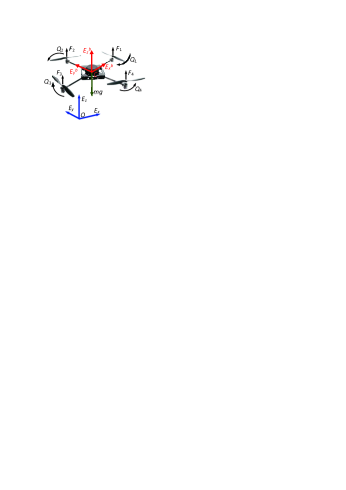
Figure 1: Forces and torques of quadrotor UAV.

Table I. UAV Parameters

Symbol	Quantity	Value
$m$	mass of UAV	$2.01kg$
$g$	gravity acceleration	$9.81m/s^{2}$
$l$	distance between rotor and gravity center	$0.2m$
$J_{\phi}$	moment of inertia about roll	$1.25kg\cdot m^{2}$
$J_{\theta}$	moment of inertia about pitch	$1.25kg\cdot m^{2}$
$J_{\psi}$	moment of inertia about yaw	$2.5kg\cdot m^{2}$
$b$	rotor force coefficient	$2.923\times 10^{-3}$
$k$	rotor torque coefficient	$5\times 10^{-4}$

5.1 Quadrotor UAV dynamics

The inertial and fuselage frames are denoted by $\Xi_{g}=\left(E_{x},E_{y},E_{z}\right)$ and $\Xi_{b}=\left(E_{x}^{b},E_{y}^{b},E_{z}^{b}\right)$, respectively; $\psi$, $\theta$ and $\phi$ are the yaw, pitch and roll angles, respectively. $F_{i}=b\omega_{i}^{2}$ is the thrust force by rotor $i$, and its reactive torque is $Q_{i}=k\omega_{i}^{2}$. The sum of the four rotor thrusts is $F=\sum\limits_{{i=1}}^{{4}}F_{i}$. The motion equations of the UAV flight dynamics are expressed by

$$\ddot{x}_{i}=h_{i}(t)+\sigma_{i}(t)$$ (20)

where, $i=1,\cdots,6$; $x_{1}=x$, $x_{2}=y$, $x_{3}=z$, $x_{4}=\psi$, $x_{5}=\theta$, $x_{6}=\phi$; $h_{1}(t)=\frac{u_{x}}{m}$, $h_{2}(t)=\frac{u_{y}}{m}$, $h_{3}(t)=\frac{u_{z}}{m}-g$, $h_{4}(t)=\frac{u_{\psi}}{J_{\psi}}$, $h_{5}(t)=\frac{u_{\theta}}{J_{\theta}}$, $h_{6}(t)=\frac{u_{\phi}}{J_{\phi}}$; $\sigma_{1}(t)=m^{-1}(-k_{x}\dot{x}+\Delta_{x})$; $\sigma_{2}(t)=m^{-1}(-k_{y}\dot{y}+\Delta_{y})$; $\sigma_{3}(t)=m^{-1}(-k_{z}\dot{z}+\Delta_{z})$; $\sigma_{4}(t)=J_{\psi}^{-1}(-k_{\psi}\dot{\psi}+\Delta_{\psi})$; $\sigma_{5}(t)=J_{\theta}^{-1}(-lk_{\theta}\dot{\theta}+\Delta_{\theta})$; $\sigma_{6}(t)=J_{\phi}^{-1}(-lk_{\phi}\dot{\phi}+\Delta_{\phi})$; $k_{x}$, $k_{y}$, $k_{z}$, $k_{\psi}$, $k_{\theta}$ and $k_{\phi}$ are the unknown drag coefficients; $(\Delta_{x},\Delta_{y},\Delta_{z})$ and $(\Delta_{\psi},\Delta_{\theta},\Delta_{\phi})$ are the uncertainties in position and attitude dynamics, respectively; $J=diag\{J_{\psi},J_{\theta},J_{\phi}\}$ is the matrix of three-axial moment of inertias; $c_{\theta}$ and $s_{\theta}$ are expressed for $\cos\theta$ and $\sin\theta$, respectively; and

$$u_{x} = (c_{\psi}s_{\theta}c_{\phi}+s_{\psi}s_{\phi})F,\text{ }u_{y}=(s_{\psi}s_{\theta}c_{\phi}-c_{\psi}s_{\phi})F,\text{ }u_{z}=c_{\theta}c_{\phi}F,$$

$$u_{\psi} = \frac{k}{b}\sum\limits_{{i=1}}^{{4}}(-1)^{i+1}F_{i},\text{ }u_{\theta}=(F_{3}-F_{1})l,\text{ }u_{\phi}=(F_{2}-F_{4})l$$ (21)

5.2 Sensing

GPS provides the global position, and a microwave Radar sensor measures velocity. An IMU gives the attitude angle and angular rate. The sensing outputs are:

$$y_{i,1}=x_{i}+d_{i}(t)+n_{i,1}(t),\text{ }y_{i.2}=\dot{x}_{i}+n_{i,2}(t)$$ (22)

where, $d_{i}(t)$ is the large error in sensing, and $\sup_{t\in[0,\infty)}\left|d_{i}(t)\right|\leq L_{i}<\infty$; $n_{i,1}(t)$ and $n_{i,2}(t)$ are noise; $i=1,\cdots,6$.

The corrector (13) and observer (14) are used to estimate ($x$, $y$, $z$, $\psi$, $\theta$, $\phi$) and the system uncertainties, respectively.

5.3 Control law design

The control laws are designed to stabilize the UAV flight. For the desired trajectory ($x_{d},y_{d},z_{d}$) and attitude angle ($\psi_{d},\theta_{d},\phi_{d}$), the error systems of position and attitude dynamics can be expressed, respectively, by

$$\ddot{e}_{p}=m^{-1}(u_{p}+\Xi_{p}+\delta_{p})$$ (23)

and

$$\ddot{e}_{a}=J^{-1}(u_{a}+\Xi_{a}+\delta_{a})$$ (24)

where, $e_{p1}=x-x_{d}$, $e_{p2}=\dot{x}-\dot{x}_{d}$, $e_{p3}=y-y_{d}$, $e_{p4}=\dot{y}-\dot{y}_{d}$, $e_{p5}=z-z_{d}$, $e_{p6}=\dot{z}-\dot{z}_{d}$; $e_{a1}=\psi-\psi_{d}$, $e_{a2}=\dot{\psi}-\dot{\psi}_{d}$, $e_{a3}=\theta-\theta_{d}$, $e_{a4}=\dot{\theta}-\dot{\theta}_{d}$, $e_{a5}=\phi-\phi_{d}$, $e_{a6}=\dot{\phi}-\dot{\phi}_{d}$;

$${\small e}_{p}{\small=}\left[\begin{array}[]{c}{\small e}_{p1}\\ {\small e}_{p3}\\ {\small e}_{p5}\end{array}\right],\text{ }u_{p}=\left[\begin{array}[]{c}u_{x}\\ u_{y}\\ u_{z}\end{array}\right],\text{ }{\small\delta_{p}}{\small=}\left[\begin{array}[]{c}{\small\Delta}_{x}-k_{x}\dot{x}\\ {\small\Delta}_{y}-k_{y}\dot{y}\\ {\small\Delta}_{z}-k_{z}\dot{z}\end{array}\right],{\small\Xi_{p}}{\small=}\left[\begin{array}[]{c}-m\ddot{x}_{d}\\ -m\ddot{y}_{d}\\ -m\ddot{z}_{d}-mg\end{array}\right]$$ (25)

and

$$e_{a}=\left[\begin{array}[]{c}e_{a1}\\ e_{a3}\\ e_{a5}\end{array}\right],\text{ }u_{a}=\left[\begin{array}[]{c}u_{\psi}\\ u_{\theta}\\ u_{\phi}\end{array}\right],\text{ }\Xi_{a}=\left[\begin{array}[]{c}-J_{\psi}\ddot{\psi}_{d}\\ -J_{\theta}\ddot{\theta}_{d}\\ -J_{\phi}\ddot{\phi}_{d}\end{array}\right],\delta_{a}=\left[\begin{array}[]{c}{\small\Delta}_{\psi}-k_{\psi}\dot{\psi}\\ {\small\Delta}_{\theta}-lk_{\theta}\dot{\theta}\\ {\small\Delta}_{\phi}-lk_{\phi}\dot{\phi}\end{array}\right]$$ (26)

5.3.1 Position dynamics control: In the position dynamics, for the desired trajectory ($x_{d},y_{d},z_{d}$), the control law

$$u_{p}=-\Xi_{p}-\widehat{\delta}_{p}-m(k_{p1}\widehat{e}_{p}+k_{p2}\widehat{\dot{e}}_{p})$$ (27)

is designed to make position error vectors $e_{p}\rightarrow\vec{0}$ and $\dot{e}_{p}\rightarrow\vec{0}$ as $t\rightarrow\infty$, where $\widehat{e}_{p1}=\widehat{x}-x_{d}$, $\widehat{e}_{p2}=\widehat{\dot{x}}-\dot{x}_{d}$, $\widehat{e}_{p3}=\widehat{y}-y_{d}$, $\widehat{e}_{p4}=\widehat{\dot{y}}-\dot{y}_{d}$, $\widehat{e}_{p5}=\widehat{z}-z_{d}$, $\widehat{e}_{p6}=\widehat{\dot{z}}-\dot{z}_{d}$ and $\widehat{\delta}_{p}$ are estimated by the correctors; $k_{p1},k_{p2}>0$; and

$$\widehat{e}_{p}=\left[\begin{array}[]{ccc}\widehat{e}_{p1}&\widehat{e}_{p3}&\widehat{e}_{p5}\end{array}\right]^{T},\widehat{\dot{e}}_{p}=\left[\begin{array}[]{ccc}\widehat{e}_{p2}&\widehat{e}_{p4}&\widehat{e}_{p6}\end{array}\right]^{T}$$ (28)

5.3.2 Attitude dynamics control: In the attitude dynamics, for the desired attitude angle ($\psi_{d},\theta_{d},\phi_{d}$), the control law

$$u_{a}=-\Xi_{a}-\widehat{\delta}_{a}-J(k_{a1}\widehat{e}_{a}+k_{a2}\widehat{\dot{e}}_{a})$$ (29)

is designed to make attitude error vectors $e_{a}\rightarrow\vec{0}$ and $\dot{e}_{a}\rightarrow\vec{0}$ as $t\rightarrow\infty$, where, $\widehat{e}_{a1}=\widehat{\psi}-\psi_{d}$, $\widehat{e}_{a2}=\widehat{\dot{\psi}}-\dot{\psi}_{d}$, $\widehat{e}_{a3}=\widehat{\theta}-\theta_{d}$, $\widehat{e}_{a4}=\widehat{\dot{\theta}}-\dot{\theta}_{d}$, $\widehat{e}_{a5}=\widehat{\phi}-\phi_{d}$, $\widehat{e}_{a6}=\widehat{\dot{\phi}}-\dot{\phi}_{d}$ and $\widehat{\delta}_{a}$ are estimated by the observers; $k_{a1},k_{a2}>0$; and

$$\widehat{e}_{a}=\left[\begin{array}[]{ccc}\widehat{e}_{a1}&\widehat{e}_{a3}&\widehat{e}_{a5}\end{array}\right]^{T},\widehat{\dot{e}}_{a}=\left[\begin{array}[]{ccc}\widehat{e}_{a2}&\widehat{e}_{a4}&\widehat{e}_{a6}\end{array}\right]^{T}$$ (30)

6 Experiment on UAV navigation and control

In this section, a UAV flight experiment is presented to demonstrate the proposed method. The UAV flight platform is explained in Figure 2. The UAV navigation and control based on the decoupling corrector and observer are implemented in the platform setup. The control system hardware is described in Figure 3, whose elements include: A Gumstix and Arduino Mega 2560 (16MHz) are selected as the driven boards; Gumstix is to collect dada from measurements; Arduino Mega is to run algorithm of estimation and control, and it sends out control commands; A XsensMTI AHRS (10 kHz) provides the 3-axial accelerations, the angular rates and the earth’s magnetic field.

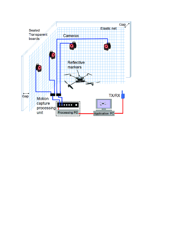
Figure 2: Platform of UAV flight control system.

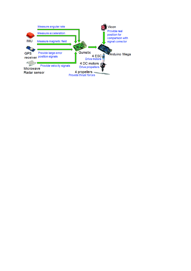
Figure 3: Control system hardware.

Real position acquisition for comparison: In order to obtain the real position for comparison with the estimation by the corrector, the output of the Vicon system with sub-millimeter accuracy is taken as the real position.

Large-error position from GPS: A low-cost GPS receiver proivdes intermittent position signals with accuracy of 10$\sim$20m. When a intermittence happens, the most recent valid readings from GPS are taken as the measured position signals.

Accurate velocity sensing: A 24GHz microwave Doppler Radar sensor is adopted to measure the velocity.

Desired flight trajectory: The UAV desired trajectory includes: 1) take off and climb; 2) then fly in a circle with the radius of 5m, the velocity of 1m/s and the altitude of 3m. The 3D desired trajectory is shown in Figure 4(a).

The corrected positions from the signal correctors and the uncertainty estimations from the observers are used in the controllers. Controllers (27) and (29) drive the UAV to track the desired trajectory. The corrector parameters: $k_{1,i}=1$, $k_{2,i}=30$, $1/\varepsilon_{c,i}=1.2$, $\alpha_{c,i}=0.1$, $i=1,2,3$. The observer parameters: $k_{3,i}=20$, $k_{4,i}=4$, $1/\varepsilon_{c,i}=1.1$, $\alpha_{o,i}=0.6$, $i=1,2,3$. The control law parameters: $k_{p1}=2.5$, $k_{p2}=4$, $k_{a1}=2.5$, $k_{a2}=4$. The position-correction performance of corrector is compared with the EKF-based GPS/Radar sensor integration.

Figure 4(a) shows the comparison of flight trajectories in 3D space, including the measured from GPS, the real from the Vicon, the desired trajectories, the estimations by the corrector and the EKF. Meanwhile, the trajectory comparisons in the three directions are shown in Figure 4(b): The measurement errors in position from GPS are about 20m. The estimate errors by the corrector are less than 0.04m, while the estimate errors by the EKF are about 5m. Thus, the large errors in position measurements are rejected by the corrector, and the effect of stochastic noises is reduced sufficiently. In addition, during a 1000s-duration flight test, no drift happened.

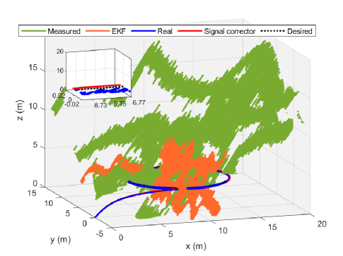
(a)

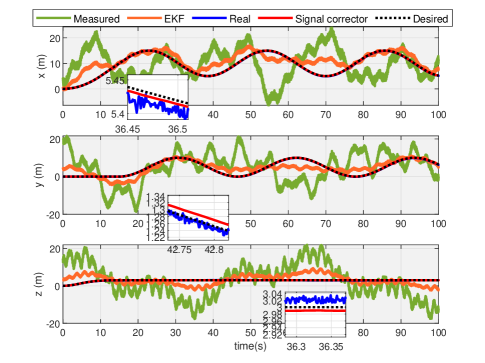
(b)

Figure 4: UAV navigation based on corrector and observer. (a) Navigation trajectories. (b) Position estimation.

Uncertainties estimation: The unexpected uncertainties exist in the UAV flight, and we cannot read these uncertainties. Therefore, the real uncertainties cannot be determined to compare with the estimate results. Here, we use a simulation to illustrate the uncertainty estimations by the observers. The unknown drag coefficients in the UAV model are supposed to be: $k_{x}=k_{y}=k_{z}=0.01$N$\cdot$s/m, $k_{\psi}=k_{\theta}=k_{\phi}=0.012$N$\cdot$s/rad. The unmodelled uncertainties are assumed as: $\Delta_{x}=0.3\sin(t)+0.2\cos(0.5t)$, $\Delta_{y}=0.2\sin(0.5t)+0.5\cos(t)$, $\Delta_{z}=0.4\sin(0.6t)+0.2\cos(t)$. Then, we can determine the real uncertainty vector ${\small\delta_{p}}$ according to (25). All the parameters in system model, correctors, observers and controllers are selected the same as those in the above experiment. Figure 5 shows that the observers can get the accurate estimation of uncertainties although much noise exists.

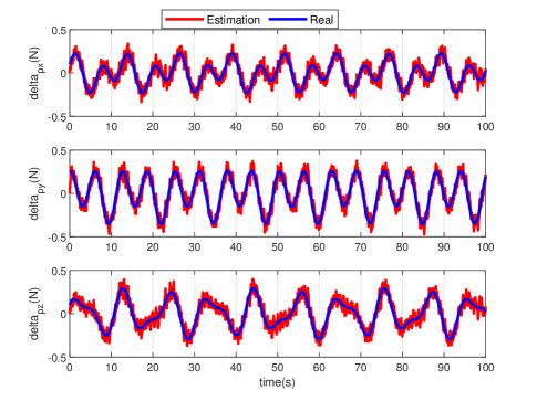
Figure 5: Uncertainty estimations.

7 Conclusions

For a class of uncertain systems with large-error sensing, according to the completely decoupling, the low-order signal corrector and observer have been developed to reject the large error in sensing and to estimate the system uncertainty. The proposed corrector and observer have been demonstrated by a UAV navigation-control experiment: it succeeded in rejecting the large errors in position sensing, and the system uncertainties were estimated accurately. The merits of the presented decoupling correction-estimation method include its strong rejection of large errors in sensing and stochastic noise, accurate estimation of uncertainties, low-order form and easy parameters selection.

Appendix

Proof of Theorem 3.1

Proof of the general signal corrector (9) in Theorem 3.1: Define the corrector error as $e_{1}=\widehat{x}_{1}-x_{1}$ and $e_{2}=\widehat{x}_{2}-x_{2}$. Then, the error system of signal corrector (9) and decoupled system (4) can be described by:

$$\dot{e}_{1} = e_{2};$$

$$\varepsilon_{c}^{3}\dot{e}_{2} = f_{c}(\varepsilon_{c}(e_{1}-d(t)),e_{2})-\varepsilon_{c}^{3}\ddot{x}_{2}(t)$$ (31)

and Eq. (31) can be rewritten as

$$\frac{d\varepsilon_{c}e_{1}}{dt/\varepsilon_{c}} = \varepsilon_{c}^{2}e_{2};$$

$$\frac{d\varepsilon_{c}^{2}e_{2}}{dt/\varepsilon_{c}} = f_{c}(\varepsilon_{c}e_{1}-\varepsilon_{c}d(t),\frac{1}{\varepsilon_{c}^{2}}\varepsilon_{c}^{2}e_{2})-\varepsilon_{c}^{3}\ddot{x}_{2}(t)$$ (32)

By choosing the following coordinate transform

$$\tau_{c}=t/\varepsilon_{c},z_{1}(\tau)=\varepsilon_{c}e_{1},z_{2}(\tau_{c})=\varepsilon_{c}^{2}e_{2},z_{c}=\left[\begin{array}[]{cc}z_{1}(\tau_{c})&z_{2}(\tau_{c})\end{array}\right]^{T};\overline{d}\left(\tau\right)=\varepsilon_{c}d\left(t\right);\overline{p}\left(\tau\right)=\varepsilon_{c}^{3}\ddot{x}_{2}(t)$$ (33)

we get $z_{c}=\Xi(\varepsilon_{c})e_{c}$, where, $\Xi(\varepsilon_{c})=diag\{\varepsilon_{c},\varepsilon_{c}^{2}\}$ and $e_{c}=[\begin{array}[]{cc}e_{1}&e_{2}\end{array}]^{{T}}$. It is rational the system acceleration is bounded, and we can assume that $\left|\ddot{x}_{2}(t)\right|\leq L_{p}<+\infty$. Then, (32) becomes

$$\frac{dz_{1}}{d\tau_{c}} = z_{2};$$

$$\frac{dz_{2}}{d\tau_{c}} = f_{c}(z_{1}-\overline{d}\left(\tau_{c}\right),\frac{1}{\varepsilon_{c}^{2}}z_{2})-\overline{p}\left(\tau_{c}\right)$$ (34)

Define $k=\frac{1}{\varepsilon_{c}^{2}}$ and

$$g(\tau_{c},z_{c}(\tau_{c}))=f_{c}(z_{1}-\overline{d}\left(\tau_{c}\right),\frac{1}{\varepsilon_{c}^{2}}z_{2})-f_{c}(z_{1},\frac{1}{\varepsilon_{c}^{2}}z_{2})-\overline{p}\left(\tau_{c}\right)$$ (35)

then, (34) can be rewritten as

$$\frac{dz_{1}}{d\tau_{c}} = z_{2};$$

$$\frac{dz_{2}}{d\tau_{c}} = f_{c}(z_{1},k\cdot z_{2})+g(\tau_{c},z_{c}(\tau_{c}))$$ (36)

From Assumption 3.3, the contraction mapping rule $\left|f_{c}(z_{1}-\overline{d}\left(\tau_{c}\right),\frac{1}{\varepsilon_{c}^{2}}z_{2})-f_{c}(z_{1},\frac{1}{\varepsilon_{c}^{2}}z_{2})\right|\leq a\left|\overline{d}\left(\tau_{c}\right)\right|^{\rho}$ holds, where, $\rho\in\left(0,1\right]$. Then, we get

$$\delta\overset{\text{define}}{=}\underset{(\tau_{c},z_{c})\in R^{3}}{\sup}\left|g(\tau_{c},z_{c}(\tau_{c}))\right|\leq a\left|\varepsilon_{c}L_{d}\right|^{\rho}+\varepsilon_{c}^{3}L_{p}\leq\varepsilon^{\rho}\delta_{c}$$ (37)

where $\delta_{c}=aL_{d}^{\rho}+L_{p}$. From Assumption 3.2, the unperturbed system

$$\frac{dz_{1}}{d\tau_{c}} = z_{2};$$

$$\frac{dz_{2}}{d\tau_{c}} = f(z_{1},k\cdot z_{2})$$ (38)

is finite-time stable. Furthermore, from Proposition 8.1 in [23], Theorem 5.2 in [24] and (37), for (36), there exist the bounded constants $\mu_{c}>0$ and $\Gamma\left(z_{c}\left(0\right)\right)>0$, such that, for $\tau_{c}\geq\Gamma\left(z_{c}\left(0\right)\right)$,

$$\left\|z_{c}\left(\tau\right)\right\|\leq\mu_{c}\delta^{\gamma_{c}}\leq\mu_{c}(\varepsilon_{c}^{\rho}\delta_{c})^{\gamma_{c}}$$ (39)

Therefore, from (33) and (39), we get

$$\|\begin{array}[]{cc}\varepsilon_{c}e_{1}&\varepsilon_{c}^{2}e_{2}\end{array}\|\leq\mu_{c}\left(\varepsilon_{c}^{\rho}\delta_{c}\right)^{\gamma_{c}}$$ (40)

for $t\geq\varepsilon_{c}\Gamma\left({\Xi(\varepsilon}_{c}{)e}_{c}\left({0}\right)\right)$. Thus, for $\forall t\in[\varepsilon_{c}\Gamma\left({\Xi(\varepsilon}_{c}{)e}_{c}\left({0}\right)\right),\infty)$, the following relations hold:

$$\left|e_{1}\right|\leq L_{c}\varepsilon^{\rho\gamma_{c}-1},\left|e_{2}\right|\leq L_{c}\varepsilon^{\rho\gamma_{c}-2}$$ (41)

where, $L_{c}=\mu_{c}\delta_{c}^{\gamma}$. Then, (41) can be written as

$$e_{1}=O(\varepsilon_{c}^{\rho\gamma_{c}-1}),e_{2}=O(\varepsilon_{c}^{\rho\gamma_{c}-2})$$ (42)

From Theorems 4.3 and 5.2 in [24], $\gamma_{c}$ can be chosen to be arbitrarily large, and

$$\gamma_{c}>3/\rho$$ (43)

is not restrictive. Accordingly, we can get $\rho\gamma_{c}-i>1$ for $i=1,2$. It implies that, for $\varepsilon_{c}\in\left(0,1\right)$, the estimate error in (42) is of higher order than the small perturbation. Consequently, the corrector can make the estimate errors sufficiently small.

Proof of the general uncertainty observer (10) in Theorem 3.1:

The decoupled system (5) from (1) can be rewritten by

$$\varepsilon_{o}\dot{x}_{2} = \varepsilon_{o}x_{3}+\varepsilon_{o}h(t)$$

$$\varepsilon_{o}^{2}\dot{x}_{3} = \varepsilon_{o}^{2}c_{\sigma}(t)$$ (44)

Define the observer error as $e_{3}=\widehat{x}_{3}-x_{2}$ and $e_{4}=\widehat{x}_{4}-x_{3}$. Then, the error system of the observer (10) and the equivalent decoupled system (44) can be described by:

$$\varepsilon_{o}\dot{e}_{3} = \varepsilon_{o}e_{4}+f_{o1}(e_{3})$$

$$\varepsilon_{o}^{2}\dot{e}_{4} = f_{o2}(e_{3})-\varepsilon_{o}^{2}c_{\sigma}(t)$$ (45)

and Eq. (45) can be rewritten as

$$\frac{de_{3}}{dt/\varepsilon_{o}} = \varepsilon_{o}e_{4}+f_{o1}(e_{3})$$

$$\frac{d\varepsilon_{o}e_{4}}{dt/\varepsilon_{o}} = f_{o2}(e_{3})-\varepsilon_{o}^{2}c_{\sigma}(t)$$ (46)

By choosing the following coordinate transform

$$\tau_{o}=t/\varepsilon_{o},z_{3}(\tau_{o})=e_{3},z_{4}(\tau_{o})=\varepsilon_{o}e_{4},z_{o}=\left[\begin{array}[]{cc}z_{3}(\tau_{o})&z_{4}(\tau_{o})\end{array}\right]^{T};\bar{c}\left(\tau_{o}\right)=\varepsilon_{o}^{2}c_{\sigma}(t)$$ (47)

we get $z_{o}=\Xi(\varepsilon_{o})e_{o}$, where, $\Xi(\varepsilon_{o})=diag\{1,\varepsilon_{o}\}$ and $e_{o}=[\begin{array}[]{cc}e_{3}&e_{4}\end{array}]^{{T}}$. Then, (46) becomes

$$\frac{dz_{3}}{d\tau_{o}} = z_{4}+f_{o1}(z_{3})$$

$$\frac{dz_{4}}{d\tau_{o}} = f_{o2}(z_{3})-\bar{c}\left(\tau_{o}\right)$$ (48)

From (47), we can get

$$\delta_{o}\overset{\text{define}}{=}\underset{\tau_{o}\in R^{+}}{\sup}\left|\bar{c}\left(\tau_{o}\right)\right|\leq\varepsilon_{o}^{2}L_{\sigma}$$ (49)

From Assumption 3.4, the unperturbed system

$$\frac{dz_{3}}{d\tau_{o}} = z_{4}+f_{o1}(z_{3})$$

$$\frac{dz_{4}}{d\tau_{o}} = f_{o2}(z_{3})$$ (50)

is finite-time stable. Furthermore, from Proposition 8.1 in [23], Theorem 5.2 in [24] and (49), for (48), there exist the bounded constants $\mu_{o}>0$ and $\Gamma\left(z_{o}\left(0\right)\right)>0$, such that, for $\tau_{o}\geq\Gamma\left(z_{o}\left(0\right)\right)$,

$$\left\|z_{o}\left(\tau_{o}\right)\right\|\leq\mu_{o}\delta_{o}^{\gamma_{o}}\leq\mu_{o}(\varepsilon_{o}^{2}L_{\sigma})^{\gamma_{o}}$$ (51)

Therefore, from (47) and (51), we get

$$\|\begin{array}[]{cc}e_{3}&\varepsilon_{o}e_{4}\end{array}\|\leq\mu_{o}\left(\varepsilon_{o}^{2}L_{\sigma}\right)^{\gamma_{o}}$$ (52)

for $t\geq\varepsilon_{o}\Gamma\left({\Xi(\varepsilon}_{o}{)e}_{o}\left({0}\right)\right)$. Thus, for $\forall t\in[\varepsilon_{o}\Gamma\left({\Xi(\varepsilon}_{o}{)e}_{o}\left({0}\right)\right),\infty)$, the following relations hold:

$$\left|e_{3}\right|\leq L_{o}\varepsilon_{o}^{2\gamma_{o}},\left|e_{4}\right|\leq L_{o}\varepsilon_{o}^{2\gamma_{o}-1}$$ (53)

where, $L_{o}=\mu_{o}L_{\sigma}^{\gamma_{o}}$. Then, (53) can be written as

$$e_{3}=O(\varepsilon_{o}^{2\gamma_{o}}),e_{4}=O(\varepsilon_{o}^{2\gamma_{o}-1})$$ (54)

From Theorems 4.3 and 5.2 in [24], $\gamma_{o}$ can be chosen to be arbitrarily large, and

$$\gamma_{o}>1$$ (55)

is not restrictive. Accordingly, we can get $2\gamma_{o}-i>1$ for $i=0,1$. It implies that, for $\varepsilon_{o}\in\left(0,1\right)$, the estimate error in (54) is of higher order than the small perturbation. Consequently, the uncertainty observer can make the estimate errors sufficiently small.

Proof of Theorem 4.1

Proof of the signal corrector (13) in Theorem 4.1:

Define the corrector error as $e_{1}=\widehat{x}_{1}-x_{1}$ and $e_{2}=\widehat{x}_{2}-x_{2}$. Then, the error system of signal corrector (13) and decoupled system (4) can be described by:

$$\dot{e}_{1} = e_{2};$$

$$\varepsilon_{c}^{3}\dot{e}_{2} = -k_{1}\left|\varepsilon_{c}(e_{1}-d(t))\right|^{\frac{\alpha_{c}}{2-\alpha_{c}}}\text{sign}\left(e_{1}-d(t)\right)-k_{2}\left|e_{2}\right|^{\alpha_{c}}\text{sign}\left(e_{2}\right)-\varepsilon_{c}^{3}\ddot{x}_{2}(t)$$ (56)

and Eq. (56) can be rewritten as

$$\frac{d\varepsilon_{c}e_{1}}{dt/\varepsilon_{c}} = \varepsilon_{c}^{2}e_{2};$$

$$\frac{d\varepsilon_{c}^{2}e_{2}}{dt/\varepsilon_{c}} = -k_{1}\left|\varepsilon_{c}e_{1}-\varepsilon_{c}d(t)\right|^{\frac{\alpha_{c}}{2-\alpha_{c}}}\text{sign}\left(e_{1}-d(t)\right)-\frac{k_{2}}{\varepsilon_{c}^{2\alpha_{c}}}\left|\varepsilon_{c}^{2}e_{2}\right|^{\alpha_{c}}\text{sign}\left(e_{2}\right)-\varepsilon_{c}^{3}\ddot{x}_{2}(t)$$ (57)

By choosing the following coordinate transform

$$\tau_{c}=t/\varepsilon_{c},z_{1}(\tau_{c})=\varepsilon_{c}e_{1},z_{2}(\tau_{c})=\varepsilon_{c}^{2}e_{2},z_{c}=\left[\begin{array}[]{cc}z_{1}(\tau_{c})&z_{2}(\tau_{c})\end{array}\right]^{T};\overline{d}\left(\tau_{c}\right)=\varepsilon_{c}d\left(t\right);\overline{p}\left(\tau_{c}\right)=\varepsilon_{c}^{3}\ddot{x}_{2}(t)$$ (58)

we get $z_{c}=\Xi(\varepsilon_{c})e_{c}$, where, $\Xi(\varepsilon_{c})=diag\{\varepsilon_{c},\varepsilon_{c}^{2}\}$ and $e_{c}=[\begin{array}[]{cc}e_{1}&e_{2}\end{array}]^{{T}}$. Then, (57) becomes

$$\frac{dz_{1}}{d\tau_{c}} = z_{2};$$

$$\frac{dz_{2}}{d\tau_{c}} = -k_{1}\left|z_{1}-\overline{d}\left(\tau_{c}\right)\right|^{\frac{\alpha_{c}}{2-\alpha_{c}}}\text{sign}\left(z_{1}-\overline{d}\left(\tau_{c}\right)\right)-\frac{k_{2}}{\varepsilon_{c}^{2\alpha_{c}}}\left|z_{2}\right|^{\alpha_{c}}\text{sign}\left(z_{2}\right)-\overline{p}\left(\tau_{c}\right)$$ (59)

Define

$$g(\tau_{c},z(\tau_{c}))=-k_{1}\left\{\left|z_{1}-\overline{d}(\tau_{c})\right|^{\frac{\alpha_{c}}{2-\alpha_{c}}}\text{sign}\left(z_{1}-\overline{d}(\tau_{c})\right)-\left|z_{1}\right|^{\frac{\alpha_{c}}{2-\alpha_{c}}}\text{sign}\left(z_{1}\right)\right\}-\overline{p}\left(\tau_{c}\right)$$ (60)

then, (59) can be rewritten as

$$\frac{dz_{1}}{d\tau_{c}} = z_{2};$$

$$\frac{dz_{2}}{d\tau_{c}} = -k_{1}\left|z_{1}\right|^{\frac{\alpha_{c}}{2-\alpha_{c}}}\text{sign}\left(z_{1}\right)-\frac{k_{2}}{\varepsilon_{c}^{2\alpha_{c}}}\left|z_{2}\right|^{\alpha_{c}}\text{sign}\left(z_{2}\right)+g(\tau_{c},z(\tau_{c}))$$ (61)

Since the contraction mapping rule $\left|x^{\rho}-\overline{x}^{\rho}\right|\leq 2^{1-\rho}\left|x-\overline{x}\right|^{\rho},\rho\in\left(0,1\right]$, we obtain

$$\delta\overset{\text{define}}{=}\underset{(\tau_{c},z_{c})\in R^{3}}{\sup}\left|g(\tau_{c},z_{c}(\tau_{c}))\right|\leq 2^{1-\frac{\alpha_{c}}{2-\alpha_{c}}}k_{1}L_{d}^{\frac{\alpha_{c}}{2-\alpha_{c}}}\varepsilon_{c}^{\frac{\alpha_{c}}{2-\alpha_{c}}}+\varepsilon_{c}^{3}L_{p}\leq\varepsilon_{c}^{\frac{\alpha_{c}}{2-\alpha_{c}}}\delta_{c}$$ (62)

where $\delta_{c}=2^{1-\frac{\alpha_{c}}{2-\alpha_{c}}}k_{1}L_{d}^{\frac{\alpha_{c}}{2-\alpha_{c}}}+L_{p}$. From [23], we know that the unperturbed system

$$\frac{dz_{1}}{d\tau_{c}} = z_{2};$$

$$\frac{dz_{2}}{d\tau_{c}} = -k_{1}\left|z_{1}\right|^{\frac{\alpha_{c}}{2-\alpha_{c}}}\text{sign}\left(z_{1}\right)-\frac{k_{2}}{\varepsilon_{c}^{2\alpha_{c}}}\left|z_{2}\right|^{\alpha_{c}}\text{sign}\left(z_{2}\right)$$ (63)

is finite-time stable. Furthermore, from Proposition 8.1 in [23], Theorem 5.2 in [24] and (62), for (61), there exist the bounded constants $\mu_{c}>0$ and $\Gamma\left(z_{c}\left(0\right)\right)>0$, such that, for $\tau_{c}\geq\Gamma\left(z_{c}\left(0\right)\right)$,

$$\left\|z_{c}\left(\tau_{c}\right)\right\|\leq\mu_{c}\delta_{c}^{\gamma_{c}}\leq\mu_{c}(\varepsilon_{c}^{\frac{\alpha_{c}}{2-\alpha_{c}}}\delta_{c})^{\gamma_{c}}$$ (64)

Therefore, from (58) and (64), we get

$$\|\begin{array}[]{cc}\varepsilon_{c}e_{1}&\varepsilon_{c}^{2}e_{2}\end{array}\|\leq\mu_{c}\left(\varepsilon_{c}^{\frac{\alpha_{c}}{2-\alpha_{c}}}\delta_{c}\right)^{\gamma_{c}}$$ (65)

for $t\geq\varepsilon_{c}\Gamma\left({\Xi(\varepsilon}_{c}{)e}_{c}\left({0}\right)\right)$. Thus, for $\forall t\in[\varepsilon_{c}\Gamma\left({\Xi(\varepsilon}_{c}{)e}_{c}\left({0}\right)\right),\infty)$, the following relations hold:

$$\left|e_{1}\right|\leq L_{c}\varepsilon_{c}^{\frac{\alpha_{c}}{2-\alpha_{c}}\gamma_{c}-1},\left|e_{2}\right|\leq L_{c}\varepsilon_{c}^{\frac{\alpha_{c}}{2-\alpha_{c}}\gamma_{c}-2}$$ (66)

where, $L_{c}=\mu_{c}\delta_{c}^{\gamma_{c}}$. Then, (66) can be written as

$$e_{1}=O(\varepsilon^{\frac{\alpha_{c}}{2-\alpha_{c}}\gamma_{c}-1}),e_{2}=O(\varepsilon^{\frac{\alpha_{c}}{2-\alpha_{c}}\gamma_{c}-2})$$ (67)

From Theorems 4.3 and 5.2 in [24], $\gamma_{c}$ can be chosen to be arbitrarily large, and

$$\gamma_{c}>\frac{6-3\alpha_{c}}{\alpha_{c}}$$ (68)

is not restrictive. Accordingly, we can get $\frac{\alpha_{c}}{2-\alpha_{c}}\gamma_{c}-i>1$ for $i=1,2$. It implies that, for $\varepsilon_{c}\in\left(0,1\right)$, the estimate error in (67) is of higher order than the small perturbation. For $\varepsilon_{c}\in(0,1)$, according to the Routh-Hurwitz Stability Criterion, $s^{2}+\frac{k_{2}}{\varepsilon_{c}^{2\alpha_{c}}}s+k_{1}$ is Hurwitz if $k_{1}>0$ and $k_{2}>0$.

Proof of the uncertainty observer (14) in Theorem 4.1:

The decoupled system (5) from (1) can be rewritten by

$$\varepsilon_{o}\dot{x}_{2} = \varepsilon_{o}x_{3}+\varepsilon_{o}h(t)$$

$$\varepsilon_{o}^{2}\dot{x}_{3} = \varepsilon_{o}^{2}c_{\sigma}(t)$$ (69)

Define the observer error as $e_{3}=\widehat{x}_{3}-x_{2}$ and $e_{4}=\widehat{x}_{4}-x_{3}$. Then, the error system of observer (14) and decoupled system (69) can be described by:

$$\varepsilon_{o}\dot{e}_{3} = \varepsilon_{o}e_{4}-k_{4}\left|e_{3}\right|^{\frac{\alpha_{o}+1}{2}}\text{sign}\left(e_{3}\right)$$

$$\varepsilon_{o}^{2}\dot{e}_{4} = -k_{3}\left|e_{3}\right|^{\alpha_{o}}\text{sign}\left(e_{3}\right)-\varepsilon_{o}^{2}c_{\sigma}(t)$$ (70)

and Eq. (70) can be rewritten as

$$\frac{de_{3}}{dt/\varepsilon_{o}} = \varepsilon_{o}e_{4}-k_{4}\left|e_{3}\right|^{\frac{\alpha_{o}+1}{2}}\text{sign}\left(e_{3}\right)$$

$$\frac{d\varepsilon_{o}e_{4}}{dt/\varepsilon_{o}} = -k_{3}\left|e_{3}\right|^{\alpha_{o}}\text{sign}\left(e_{3}\right)-\varepsilon_{o}^{2}c_{\sigma}(t)$$ (71)

By choosing the following coordinate transform

$$\tau_{o}=t/\varepsilon_{o},z_{3}(\tau_{o})=e_{3},z_{4}(\tau_{o})=\varepsilon_{o}e_{4},z_{o}=\left[\begin{array}[]{cc}z_{3}(\tau_{o})&z_{4}(\tau_{o})\end{array}\right]^{T};\bar{c}\left(\tau_{o}\right)=\varepsilon_{o}^{2}c_{\sigma}(t)$$ (72)

we get $z_{o}=\Xi(\varepsilon_{o})e_{o}$, where, $\Xi(\varepsilon_{o})=diag\{1,\varepsilon_{o}\}$ and $e_{o}=[\begin{array}[]{cc}e_{3}&e_{4}\end{array}]^{{T}}$. Then, (71) becomes

$$\frac{dz_{3}}{d\tau_{o}} = z_{4}-k_{4}\left|z_{3}\right|^{\frac{\alpha_{o}+1}{2}}\text{sign}\left(z_{3}\right)$$

$$\frac{dz_{4}}{d\tau_{o}} = -k_{3}\left|z_{3}\right|^{\alpha_{o}}\text{sign}\left(z_{3}\right)-\bar{c}\left(\tau_{o}\right)$$ (73)

From (72), we can get

$$\delta_{o}\overset{\text{define}}{=}\underset{\tau_{o}\in R^{+}}{\sup}\left|\bar{c}\left(\tau_{o}\right)\right|\leq\varepsilon_{o}^{2}L_{\sigma}$$ (74)

From Theorem 1 in [27], we know that the unperturbed system

$$\frac{dz_{3}}{d\tau_{o}} = z_{4}-k_{4}\left|z_{3}\right|^{\frac{\alpha_{o}+1}{2}}\text{sign}\left(z_{3}\right)$$

$$\frac{dz_{4}}{d\tau_{o}} = -k_{3}\left|z_{3}\right|^{\alpha_{o}}\text{sign}\left(z_{3}\right)$$ (75)

is finite-time stable. Furthermore, from Proposition 8.1 in [23], Theorem 5.2 in [24] and (74), for (73), there exist the bounded constants $\mu_{o}>0$ and $\Gamma\left(z_{o}\left(0\right)\right)>0$, such that, for $\tau_{o}\geq\Gamma\left(z_{o}\left(0\right)\right)$,

$$\left\|z_{o}\left(\tau_{o}\right)\right\|\leq\mu_{o}\delta_{o}^{\gamma_{o}}\leq\mu_{o}(\varepsilon_{o}^{2}L_{\sigma})^{\gamma_{o}}$$ (76)

Therefore, from (72) and (76), we get

$$\|\begin{array}[]{cc}e_{3}&\varepsilon_{o}e_{4}\end{array}\|\leq\mu_{o}\left(\varepsilon_{o}^{2}L_{\sigma}\right)^{\gamma_{o}}$$ (77)

for $t\geq\varepsilon_{o}\Gamma\left({\Xi(\varepsilon}_{o}{)e}_{o}\left({0}\right)\right)$. Thus, for $\forall t\in[\varepsilon_{o}\Gamma\left({\Xi(\varepsilon}_{o}{)e}_{o}\left({0}\right)\right),\infty)$, the following relations hold:

$$\left|e_{3}\right|\leq L_{o}\varepsilon_{o}^{2\gamma_{o}},\left|e_{4}\right|\leq L_{o}\varepsilon_{o}^{2\gamma_{o}-1}$$ (78)

where, $L_{o}=\mu_{o}L_{\sigma}^{\gamma_{o}}$. Then, (78) can be written as

$$e_{3}=O(\varepsilon_{o}^{2\gamma_{o}}),e_{4}=O(\varepsilon_{o}^{2\gamma_{o}-1})$$ (79)

From Theorems 4.3 and 5.2 in [24], $\gamma_{o}$ can be chosen to be arbitrarily large, and

$$\gamma_{o}>1$$ (80)

is not restrictive. Accordingly, we can get $2\gamma_{o}-i>1$ for $i=0,1$. It implies that, for $\varepsilon_{o}\in\left(0,1\right)$, the estimate error in (79) is of higher order than the small perturbation. According to the Routh-Hurwitz Stability Criterion, $s^{2}+k_{4}s+k_{3}$ is Hurwitz if $k_{3}>0$ and $k_{4}>0$.

This concludes the proof. $\blacksquare$

References

• [1] Kwak, J., & Sung, Y. (2018). Autonomous UAV Flight Control for GPS-Based Navigation, IEEE Access, 6, 37947-37955.
• [2] Grip, H.F., Fossen, T.I., Johansen, T.A., & Saberi, A. (2015). Globally exponentially stable attitude and gyro bias estimation with application to GNSS/INS integration. Automatica, 51, 158-166.
• [3] Hsu, L.T. (2018). Analysis and modeling GPS NLOS effect in highly urbanized area, GPS Solutions, 22(7), 1-12.
• [4] Liu, Y.C., Bianchin, G. & Pasqualetti, F., (2020). Secure trajectory planning against undetectable spoofing attacks. Automatica, 112, 108655.
• [5] Freda, P., Angrisano, A., Gaglione, S., & Troisi, S. (2015). Time-differenced carrier phases technique for precise GNSS velocity estimation, GPS Solutions, 19, 335-341.
• [6] Serrano, L., Kim, D., Langley, R.B., Itani, K., & Ueno, M. (2004). A GPS velocity sensor: How accurate can it be? – A first look, ION NTM, San Diego, CA.
• [7] Griffiths, H.D. (2019). Small-and Short-Range Radar Systems GL Charvat, CRC Press, Taylor & Francis Group, 6000 Broken Sound Parkway NW, Suite 300, Boca Raton, FL 33487-2742, USA. 2017. Distributed by Taylor & Francis Group, 2 Park Square, Milton Park, Abingdon, OX14 4RN, UK. xxvii; 385pp. Illustrated£ 77.99.(20% discount available to RAeS members via www. crcpress. com using AKQ07 promotion code). ISBN 978-1-138-07763-8. The Aeronautical Journal, 123(1266), pp.1306-1306.
• [8] Levant, A. (2003). High-order sliding modes, differentiation and output-feedback control, International Journal of Control, 76(9/10), 924-941.
• [9] Levant, A., & Livne, M. (2018). Globally convergent differentiators with variable gains, Int. J. Control, vol. 91, 1994-2008.
• [10] Levant, A. and Yu, X. (2018). Sliding-mode-based differentiation and filtering. IEEE Transactions on Automatic Control, 63(9), pp.3061-3067.
• [11] Khalil, H.K. (2017). Cascade high-gain observers in output feedback control, Automatica, vol. 80, 110-118.
• [12] Khalil, H.K., & Priess, S. (2016). Analysis of the use of low-pass filters with high-gain observers, IFAC-PapersOnLine, vol. 49, no. 18, 488-492.
• [13] Wang, X., Chen, Z., & Yang, G. (2007). Finite-time-convergent differentiator based on singular perturbation technique. IEEE Transactions on Automatic Control, 52(9), 1731–1737.
• [14] Rogne, R.H., Bryne, T.H., Fossen, T.I., & Johansen, T.A. (2020). On the usage of low-cost mems sensors, strapdown inertial navigation, and nonlinear estimation techniques in dynamic positioning. IEEE J. Ocean. Eng., 46(1), 24-39.
• [15] Hamel, T., Hua, M.D., & Samson, C. (2020) December. Deterministic observer design for vision-aided inertial navigation. In 2020 59th IEEE Conference on Decision and Control (CDC), 1306-1313
• [16] Ludwig, S.A., & JimΓ©nez, A,R. (2018). Optimization of gyroscope and accelerometer/magnetometer portion of basic attitude and heading reference system, 2018 IEEE International Symposium on Inertial Sensors and Systems (INERTIAL), Moltrasio, Italy.
• [17] Deo, V.A., Silvestre, F. and Morales, M. (2020). Flight performance monitoring with optimal filtering applications. The Aeronautical Journal, 124(1272), pp.170-188.
• [18] Lin, C.L., Li, J.C., Chiu, C.L., Wu, Y.W. and Jan, Y.W. (2022). Gyro-stellar inertial attitude estimation for satellite with high motion rate. The Aeronautical Journal, pp.1-15.
• [19] Stovner, B.N., Johansen, T.A., Fossen, T.I., & SchjΓΈlberg, I. (2018). Attitude estimation by multiplicative exogenous Kalman filter. Automatica, 95, 347-355.
• [20] Wang, Y. and Zheng, X. (2019). Path following of Nano quad-rotors using a novel disturbance observer-enhanced dynamic inversion approach. The Aeronautical Journal, 123(1266), pp.1122-1134.
• [21] Liu, J., Vazquez, S., Wu, L., Marquez, A., Gao, H., & Franquelo, L.G. (2017). Extended state observer-based sliding-mode control for three-phase power converters, IEEE Trans. Ind. Electron., 64(1), 22 - 31.
• [22] Wang, X.H., Chen, Z.Q. and Yuan, Z.Z. (2004). Output tracking based on extended observer for nonlinear uncertain systems. Control and Decision, 19(10), pp.1113-1116.
• [23] Bhat, S.P., & Bernstein, D.S. (2005). Geometric homogeneity with applications to finite-time stability, Math. Control, Signals, Syst., 17(2), 101-127.
• [24] Bhat, S.P., & Bernstein, D.S. (2000). Finite-time stability of continuous autonomous systems, Siam J. Control Optim., 38(3), 751-766.
• [25] Crassidis, J.L. (2017). Introduction to the Special Issue on the Kalman Filter and Its Aerospace Applications, J. Guid. Control Dyn., 40(9), 2137-2137.
• [26] Kahlil, H.K. (2002). Nonlinear Systems, 3rd ed. Englewood Cliffs, NJ, USA: Prentice-Hall, 381-449.
• [27] Wang, X., & Lin, H. (2012). Design and frequency analysis of continuous finite-time-convergent differentiator. Aerospace Science and Technology, 18(1), 69-78.