Transfer learning for affordable and high quality tunneling splittings from instanton calculations

Abstract

The combination of transfer learning (TL) a low level potential energy surface (PES) to a higher level of electronic structure theory together with ring-polymer instanton (RPI) theory is explored and applied to malonaldehyde. The RPI approach provides a semiclassical approximation of the tunneling splitting and depends sensitively on the accuracy of the PES. With second order Møller-Plesset perturbation theory (MP2) as the low-level (LL) model and energies and forces from coupled cluster singles, doubles and perturbative triples (CCSD(T)) as the high-level (HL) model, it is demonstrated that CCSD(T) information from only 25 to 50 judiciously selected structures along and around the instanton path suffice to reach HL-accuracy for the tunneling splitting. In addition, the global quality of the HL-PES is demonstrated through a mean average error of 0.3 kcal/mol for energies up to 40 kcal/mol above the minimum energy structure (a factor of 2 higher than the energies employed during TL) and $<2$ cm^-1 for harmonic frequencies compared with computationally challenging normal mode calculations at the CCSD(T) level.

University of Basel]Department of Chemistry, University of Basel, Klingelbergstrasse 80 , CH-4056 Basel, Switzerland ETH Zurich]Laboratory of Physical Chemistry, ETH Zurich, 8093 Zurich, Switzerland University of Basel]Department of Chemistry, University of Basel, Klingelbergstrasse 80 , CH-4056 Basel, Switzerland

1 Introduction

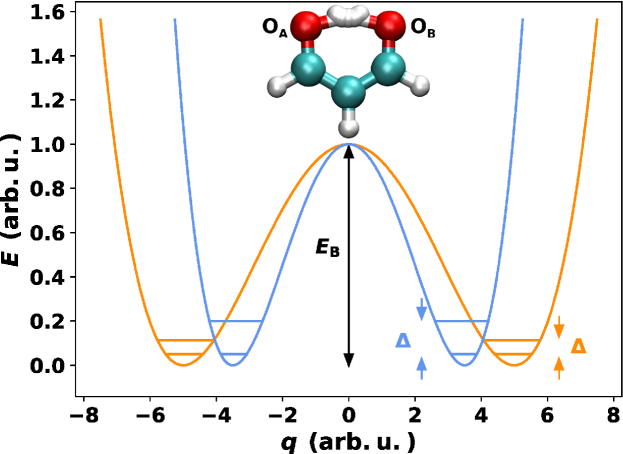
Tunneling splittings are exquisitely sensitive to the accuracy of a molecular potential energy surface (PES). The nuclear wave-functions corresponding to the two or multiple quantum mechanical bound states involved in the split energy levels probe an extended region on the underlying PES. Furthermore, the tunneling splitting also informs about the barrier height and the shape of the PES in the region connecting the two wells, see Figure 1. Due to all the above, tunneling splittings constitute a meaningful and stringent test of the level of theory at which the underlying PESs were calculated and the accuracy of their representation required for simulations from which the splittings are determined.

Figure 1: Schematic illustration of two symmetric double-well potentials with the same energy barrier $E_{\rm B}$ but differing curvatures and tunneling splittings $\Delta$. Malonaldehyde and its instanton path are shown.

Even if a PES is given, accurate computation of tunneling splittings for multidimensional systems from quantum-based methods itself is a formidable task. The ring-polymer instanton (RPI) approach provides a semiclassical approximation of a tunneling process and can be used to calculate tunneling splittings in molecular systems.^{1, 2, 3, 4} As was shown for the formic acid dimer⁴, it is necessary to include all degrees of freedom of the molecule for a quantitative comparison with experiment. This often means that the (semiclassical) full-dimensional instanton approximation is more accurate than a reduced-dimensional quantum calculation. Instanton theory is based on the path-integral formulation of quantum mechanics and is formally exact only in the limit of $\hbar\rightarrow 0$.⁵ In many previous studies it has been shown to give predictions within about 20% of fully quantum-mechanical calculations using the same PES for typical molecular systems, as long as the barrier height is significantly higher than the zero-point energy along the tunneling mode.^{1, 4, 6} Instanton calculations which, contrary to exact quantum calculations such as wave-function propagation,^{7, 8} scale well with system size, are often used in combination with analytical, full-dimensional PESs. Path-integral molecular dynamics (PIMD) simulations also scale well with system size but are considerably more expensive than an instanton calculation.^{9, 10}

In principle it is possible to implement the instanton approach using on-the-fly ab-initio electronic structure calculations.^{11, 12} However, because energies, gradients and Hessians are needed for each ring-polymer bead, this may be impractical for medium-sized molecules if high accuracy from coupled cluster with perturbative triples (CCSD(T)) level of theory is sought. More recent work has been devoted to combining machine learning (ML) and instanton theory to reduce overall computational expense. Gaussian process regression (GPR) has been used to obtain a local fit of the PES around the dominant tunneling pathway to calculate rate constants.¹³ It has been shown that the GPR rate constants are on par with the ab initio results, however, reducing the number of required electronic structure calculations by an order of magnitude. Similarly, instanton rate theory has been combined with NNs to obtain the PES more efficiently as compared to the on-the-fly approach^{14, 15}.

As an alternative, full-dimensional PESs can now be constructed for medium-sized molecules from which tunneling splittings can also be determined using the instanton approach. The generation of ML PESs based on large data sets of ab initio data is a challenging task¹⁶ and accuracy as well as the level of theory of the PES is of crucial importance for the accurate determination of tunneling splittings. The “gold standard” CCSD(T) approach scales as $N^{7}$ (with $N$ being the number of basis functions)¹⁷ which quickly becomes computationally prohibitive for generating data to build a full-dimensional PESs even for relatively small molecules. To avoid the need for calculating large ab initio data sets at high levels of theory transfer learning (TL) ^{18, 19, 20} and related $\Delta$-ML²¹ were shown to be data and cost-effective alternatives^{22, 23, 24, 25, 26, 27}.

The combination of TL and instanton theory appears particularly appealing as the instanton path (IP) can be determined on a low-level PES, which gives a rough approximation to the true tunneling path, and can be included (and iteratively refined if needed) into the TL data set. Additionally, the IP is inherently local and, thus, allows concentrating on improving only a small part of a PES. While instanton theory has been used in combination with ML schemes^{13, 28, 15}, the present work demonstrates the first combination of instanton theory with TL. The capability of the combined approach is demonstrated for the extensively studied malonaldehyde system exhibiting intramolecular hydrogen transfer (HT).

Ring Polymer Instanton theory has been employed to calculate the tunneling splitting of malonaldehyde on a permutationally invariant polynomial (PIP) PES fitted to 11147 near basis-set-limit frozen-core CCSD(T) electronic energies²⁹. The splitting was found to be 25 cm^-1 with RPI ⁶ as well as with a strongly related instanton method ³⁰. The same PES was also used to calculate tunneling splittings using the fixed-node diffusion Monte Carlo (DMC) method giving 21.6 cm^-1 with a statistical uncertainty of 2 to 3 cm^-1.²⁹ For DT, computed values on the PIP PES are 3.3 and 3.4 cm^-1 using RPI⁶ and the related instanton method³⁰, and $3.0\pm 2-3$ cm^-1 from DMC simulations.²⁹ The tunneling splitting from RPI calculations on a LASSO fit to CCSD(T)(F12*) energies was found to be 19.3 cm^-1.^{6, 31} To validate such computations, direct comparison with experiment is also of interest. Reliable tunneling splittings from experiment are only available for a few select systems^{32, 33, 34, 35, 36, 37, 38, 39}. For malonaldehyde, the experimentally determined tunneling splitting is 21.583 cm^-1 and 2.915 cm^-1 for HT and deuterium transfer (DT), respectively^{32, 33, 40}. Although these results are not in perfect agreement with experiment, they are close enough that spectroscopic assignments can be made and provide detailed mechanistic information about the tunneling process.

The purpose of the present work is to develop and quantitatively assess an evidence-based procedure to determine reliable tunneling splittings by combining transfer learned PESs with instanton calculations. It is shown that this can dramatically reduce the cost of the overall simulation in comparison to working with ab initio potentials. The work is structured as follows. First, the methods and the generation of the data sets are presented. This is followed by a thorough evaluation of the accuracy of the transfer leaned PESs in terms of tunneling splittings and harmonic frequencies. Finally, the results are discussed and conclusions are drawn.

2 Methods

2.1 Ring-Polymer Instanton Theory

In a one-dimensional model, instanton theory is strongly related to the WKB approximation⁴¹. Its main advantage, however, is that it can also be applied to multidimensional systems, in which it locates the uniquely defined optimal tunneling pathway.⁴² This pathway, known as the instanton, is defined as a long imaginary-time $\tau\rightarrow\infty$ path connecting two degenerate wells which minimizes the action, $S$. In computations, the path is located using an efficient ring-polymer optimization based on discretizing the path into $N$ ring-polymer beads and taking the limit $N\rightarrow\infty$ (typically on the order of 1000 is sufficient for convergence). The action is determined by the distance between neighbouring beads as well as the potential-energy of each bead, i.e. it uses information along the IP. Full technical details are presented in previous work.^{1, 2} In general, the IP is not equivalent to the minimum-energy pathway (MEP) and will not even pass through a saddle point. This is because the instanton finds a compromise between length and height to optimize the tunneling path. Unlike PIMD or DMC, no random numbers or statistical errors are involved and so the instanton (once it is converged with $\tau\rightarrow\infty$ and $N/\tau\rightarrow\infty$) is in principle uniquely determined by the PES.

Once the IP has been located, fluctuations around the path are computed to second order and the information is combined into the term $\Phi$, i.e. this is based on information around the IP. For this, one requires the Hessians (second-derivative matrix of PES) at each bead. The final prediction for the tunneling splitting (in a double-well system) is given by

$$\Delta=\frac{2\hbar}{\Phi}\sqrt{\frac{S}{2\pi\hbar}}\,\mathrm{e}^{-S/\hbar}.$$ (1)

Because $S$ appears in the exponent it is particularly important to determine this quantity with high accuracy.

The method has also been generalized to treat tunneling in systems with multiple (more than two) wells ^{43, 3} and in cases with non-degenerate wells for instance due to asymmetric isotopic substitution.⁶ The approach outlined in this work is, in principle, also applicable to these extensions.

2.2 Machine Learning

All PESs used in this work are represented with a high-dimensional neural network (NN) of the PhysNet⁴⁴ architecture. PhysNet is a ‘message-passing’⁴⁵ NN that employs learnable descriptors of the atomic environments to predict individual atomic energy contributions $E_{i}$ and partial charges $q_{i}$. The descriptors are initialized as ${\bf x}_{i}^{0}={\bf e}_{Z_{i}}$, where ${\bf e}_{Z_{i}}$ corresponds to a parameter vector defined by the nuclear charge $Z_{i}$, i.e. atoms of the same element share the same descriptor. The descriptor is then iteratively updated and refined to best describe the local chemical environment of each atom $i$ by passing ‘messages’ between atoms within a cut-off $r_{\rm cut}$ following

$${\bm{x}}_{i}^{l+1}={\bm{x}}_{i}^{l}+\sum_{r_{ij}<r_{cut}}\mathcal{F}({\bm{x}}_{i}^{l},{\bm{x}}_{j}^{l},r_{ij}).$$ (2)

where $r_{\rm cut}$ was 10 Å. Here, ${\bm{x}}_{i}^{l}$ and ${\bm{x}}_{j}^{l}$ are the descriptors of atoms $i$ and $j$ at iteration $l$, $r_{ij}$ is their interatomic distance and $\mathcal{F}({\bm{x}}_{i}^{l},{\bm{x}}_{j}^{l},r_{ij})$ is the ‘message-passing’ function (for details see Ref. 44). Because only pairwise distances are used to encode the atoms’ chemical environment and summation is commutative, the resulting descriptors (and thus the PES) are invariant with respect to translation, rotation and permutation of identical atoms, which is of particular importance when describing tunneling between degenerate wells. The descriptors are then used to predict partial charges $q_{i}$ (which are corrected to ensure total charge conservation) and the total energy of the chemical system by summation of the atomic contributions and explicitly including long-range electrostatics according to

$$E=\sum_{i}E_{i}+k_{e}\sum_{i=1}^{N}\sum_{j>i}^{N}\frac{q_{i}q_{j}}{r_{ij}}$$ (3)

Here, $k_{e}$ represents Coulomb’s constant and the second term involving $\frac{q_{i}q_{j}}{r_{ij}}$ is damped to avoid numerical instabilities caused by the singularity at $r_{ij}=0$ (for details refer to Ref. 44). The forces ${\bm{F}}$ and Hessians ${\bm{H}}$ can be obtained analytically using reverse mode automatic differentiation⁴⁶ as implemented in Tensorflow⁴⁷.

The learnable parameters of PhysNet are fitted to reference ab initio energies, forces and dipole moments following the strategy outlined in Reference 44. The partial charges $q_{i}$ are fitted to the ab initio dipole moment ($\mu=\sum_{i}^{N}q_{i}{\bm{r}_{i}}$) and explicitly enter the energy expression (see equation 3). In the present work, the TL scheme is employed whereby the parameters of a low-level (LL) treatment are used as a meaningful initial guess and are fine-tuned using higher-level information. For TL, the learning rate is reduced from $10^{-3}$ (as for learning a model from scratch) to $10^{-4}$. The LL in the present work is the full-dimensional PES for malonaldehyde at the MP2/aug-cc-pVTZ level of theory (henceforth, PhysNet MP2 PES) which is available from previous work and was trained on $\sim 70000$ reference structures.²² This PhysNet PES has a barrier for HT of 2.79 kcal/mol which compares to a reference value of 2.74 kcal/mol calculated at the MP2/aug-cc-pVTZ level of theory and the reference harmonic frequencies are reproduced with a root-mean-square deviation (RMSD) of 3.6 cm^-1. The high-level (HL) treatment is the considerably higher and computationally much more demanding CCSD(T)/aug-cc-pVTZ level of theory at which energies, forces and dipole moments are calculated using Molpro⁴⁸ for all data points used in TL.

2.3 Data Set Generation

Transfer learning requires high-level energies, forces and dipole moments for selected geometries of the system considered and ideally cover all spatial regions relevant for the observable(s) of interest. Without additional a priori information it is advantageous to generate an initial pool of structures which can be used for TL to fine-tune the LL treatment. When selecting configurations, it is not necessary to sample both potential wells since PhysNet handles this symmetry by construction. Here, the initial pool contained 862 malonaldehyde configurations consisting of:

• 111 geometries along the MEP of the PhysNet MP2 PES.

• 110 geometries along the IP of the PhysNet MP2 PES.

• 111 geometries along the IP determined on a PES that was transfer learned by using CCSD(T) information of the 111 MEP geometries (see above) to have an energy barrier closer to the ab initio CCSD(T) barrier.

• 280 geometries obtained from normal mode sampling (NMS) around the equilibrium geometry. For this purpose, normal mode vectors and corresponding force constants are determined ab initio at the MP2/aug-cc-pVTZ level of theory.

• 240 geometries around the IP as obtained from NMS.

• 10 geometries along the IP of TL₁ (see Section 3.2).

This data set is referred to as the “Extended Data Set” and transfer learned models using it are called TL_ext. To probe the dependence of barrier heights and tunneling splittings on details of the training, ten independent models were trained on different splits of the data for TL_ext (and all the subsequent TLs). For each of the ten resulting PESs an instanton calculation was carried out. From this information, averages and standard deviations for the barrier heights and tunneling splittings were determined.

After validating the performance of TL_ext from instanton calculations on each of the independently trained models, smaller subsets of the Extended Data Set were selected, employed for TL and subsequent tunneling splitting calculations.

3 Results

To set the stage, the tunneling splittings for malonaldehyde were calculated on the PhysNet MP2 PES using RPI theory. The tunneling splitting calculations were carried out with three different values of the imaginary time, $\tau$, corresponding to effective ‘temperatures’ $T=\hbar/k_{B}\tau\in[50,25,12.5]$ K and with different numbers of beads $N\in[2^{5},..,2^{12}]$ to ensure convergence. Formally the instanton result is defined in the low-temperature limit, which is equivalent to infinitely-long imaginary times. The results are summarized in Table S1. A tunneling splitting of 96 cm^-1 is obtained compared with 25 cm^-1 from instanton calculations^{30, 6} on the PIP-representation²⁹ of the CCSD(T) reference data and 21.6 cm^-1 from experiments.^{32, 33, 40} This illustrates the insufficient quality of the MP2 level of theory to capture tunneling splittings correctly. For the following, all instanton calculations were carried out with $N=4096$ beads at an effective temperature of $T=25$ K, which was found to be more than sufficient for convergence of $\Delta$ to two significant figures.

Figure 2: Data sets used for TL projected onto a 2D cut through the TL_ext PES spanned by the O–O distance and the reaction coordinate $q=r_{\rm O_{A}H}-r_{\rm O_{B}H}$, for labels see Fig. 1. The Extended Data Set (862 structures, gray circles) is shown together with sets for TL₀ (25 structures, yellow crosses), TL₁ (50 structures, turquoise circles), and TL₂ (100 structures, salmon squares). The MEP and the instanton path (as determined on the TL_ext PES) are marked with a dash-dotted and a dashed line, respectively. The IP on the PhysNet MP2 PES is the white dashed line and clearly differs from that (black dashed) on the CCSD(T) PES.

3.1 Performance of TL_ext

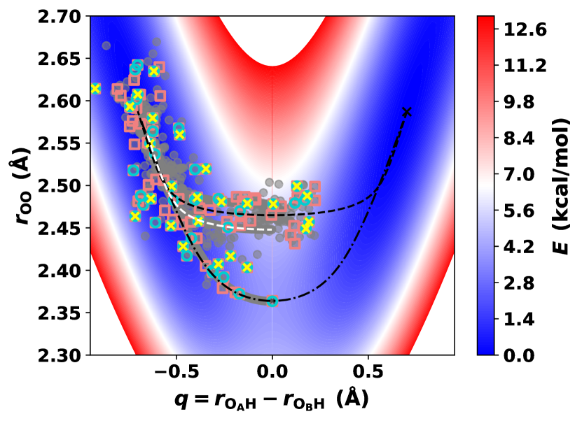
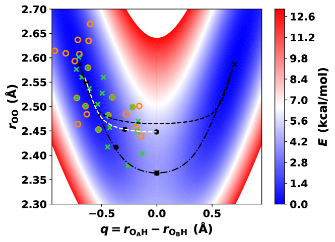
As a reference for the following exploration, the performance of TL_ext using the full set of 862 energies, forces and dipole moments determined at the CCSD(T)/aug-cc-pVTZ level is first assessed. These geometries are shown as a projection onto the PES spanned by the O–O distance and the reaction coordinate $q=r_{\rm O_{A}H}-r_{\rm O_{B}H}$ in Figure 2 (gray circles). As the PES is symmetric with respect to $q=0$, the same geometry appears to the left and to the right of the mirror plane. The Extended Data Set was split according to $\sim 80/10/10$ % into training/validation/test sets, from which the test sets were used only for testing. Across the 10 TL models, the separate test sets were predicted on average with MAE($E$) $\approx 0.006$, RMSE($E$) $\approx 0.009$ kcal/mol, MAE($F$) $\approx 0.03$ and RMSE($F$) $\approx 0.07$ kcal/mol/Å. The average barrier height on the ten transfer-learned PESs ($\langle{\rm TL}_{\rm ext}\rangle$) was $E_{\rm B}=3.8945\pm 0.0006$ kcal/mol which compares with an ab initio barrier of 3.8948 kcal/mol determined at the CCSD(T)/aug-cc-pVTZ level of theory determined from present calculations. The RPI tunneling splittings for HT and DT were $\Delta_{\rm H}=25.3\pm 0.2$ cm^-1 and $\Delta_{\rm D}=3.7\pm 0.03$ cm^-1, respectively, see Table 1 and S2. These results compare with computed splittings on the PIP representation of CCSD(T)/aug-cc-pVTZ reference calculations using instanton calculations that yield 25/3.4 cm^{-130, 6} and experimental splittings of 21.6/2.9 cm^-1.^{32, 33, 40} Hence, the transfer-learned PES using fewer than 1000 higher level CCSD(T)/aug-cc-pVTZ energies and forces together with the same method for determining the tunneling splitting performs on par with calculations on the PIP representation of the $\sim 11000$ CCSD(T)/aug-cc-pVTZ energies.²⁹ Based on this it is of much practical interest to further reduce the number of HL calculations required to achieve the same result. Therefore, in a next step, different subsets of the Extended Data Set are considered and used for TL to arrive at an ideally small number of HL points while still retaining the accuracy in tunneling splittings from instanton calculations.

	$N_{\rm data}$	$E_{\rm B}$	$\Delta_{\rm H}$	$S/\hbar$	$\Phi$
MP2	70k	2.7889	96.3	4.502	42.770
$\langle{\rm TL}_{0}\rangle$	25	$3.8925\pm 0.0119$	$23.4\pm 1.9$	$5.749\pm 0.026$	$57.405\pm 4.486$
$\langle{\rm TL}_{1}\rangle$	50	$3.8974\pm 0.0161$	$24.9\pm 1.1$	$5.764\pm 0.012$	$53.096\pm 2.375$
$\langle{\rm TL}_{2}\rangle$	100	$3.8941\pm 0.0021$	$25.2\pm 0.5$	$5.748\pm 0.005$	$53.053\pm 1.156$
$\langle{\rm TL}_{\rm ext}\rangle$	862	$3.8945\pm 0.0006$	$25.3\pm 0.2$	$5.743\pm 0.002$	$53.241\pm 0.454$

Table 1: Energy barriers $E_{\mathrm{B}}$ (kcal/mol), tunneling splittings $\Delta$ (in cm^-1) at $T=25$ K and with $N=4096$, action $S/\hbar$ and fluctuation factor $\Phi$ (in a.u. of time $\hbar/E_{h}$) for malonaldehyde determined from TL_ext and TL_0,1,2 PESs. The ab initio barrier height for HT at the CCSD(T)/aug-cc-pVTZ level of theory is 3.8948 kcal/mol.

3.2 Performance on Smaller Datasets: TL₀, TL₁, and TL₂

From the Extended Data Set containing 862 geometries, different subsets were extracted. The size of the data set has to be chosen small enough for efficient computation but sufficiently large to still cover the appropriate regions of configurational space probed by the instanton calculation.

TL₀: To check whether a considerably smaller data set suffices as a starting point, ten TLs were preformed on a data set containing only 25 geometries: a) 5 IP geometries (approximately equally spaced) determined on a PES that was transfer learned to have a barrier closer to the ab initio CCSD(T) barrier; b) 10 geometries, each, selected from the NMS around the equilibrium geometry and the IP. This can be done by selecting geometries based on a RMSD criterion on the $n$ atomic positions ($\sqrt{\frac{1}{n}\sum_{i=1}^{n}||v_{i}-w_{i}||^{2}}$ where $v_{i}$ and $w_{i}$ are two sets of Cartesian coordinates of atom $n$), which was done as follows for both groups of geometries that were generated with NMS. Starting from a random geometry, new geometries are added iteratively if the RMSD with respect to the selected ones is larger than a threshold. For this reason, the threshold is maximized to include 10 geometries. Note that no MEP geometries are added. The data set for TL₀ are the yellow crosses in Figure 2.

With this smallest subset the barrier height of the (ensemble of the) transfer learned PES $\langle{\rm TL}_{0}\rangle$ is $E_{\rm B}=3.8925\pm 0.012$ kcal/mol which is, within errors, close to the target value of 3.8948 kcal/mol determined at the CCSD(T)/aug-cc-pVTZ level. 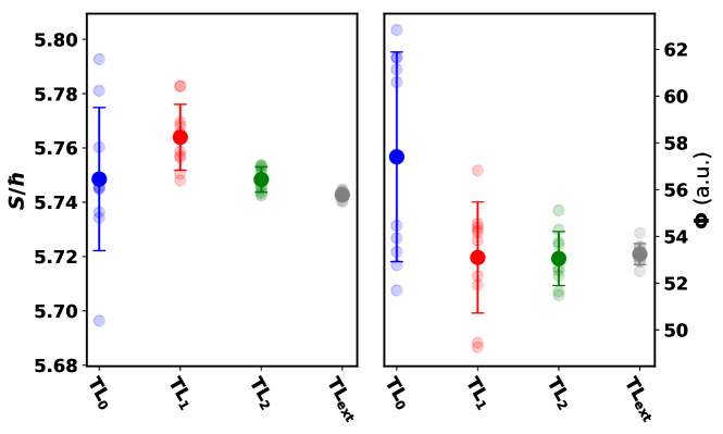From 10 independent instanton calculations the average splitting is $\Delta_{\rm H}=23.4\pm 1.9$ cm^-1 which is $\sim 2$ cm^-1 below that from the simulations on the TL_ext PES but still within statistical fluctuation. Comparing the action $S/\hbar$ of the IPs on TL₀ and TL_ext shows that they are comparable ($5.743\pm 0.002$ vs. $5.749\pm 0.026$) and even identical within the error bars. However, the uncertainty on TL₀ is larger by an order of magnitude compared with that on TL_ext. Thus, the action, $S/\hbar$, of the path is clearly less well defined on TL₀. For the fluctuation factor $\Phi$ the differences are considerably larger between the two families of PESs. Still, the values themselves are within error bounds but again, the fluctuation around the mean for TL₀ is ten times larger than that for the TL_ext PESs. This conclusion also hold for DT, see Table S2. Overall, using only 25 additional data points as done for TL₀ already yields encouraging results for the barrier height and tunneling splittings. To explore further improvements new points were added and the process was repeated.

Figure 3: Tunneling splittings for H- and D-transfer (left and right panels) from all TL PESs (transparent circles). The corresponding averages (opaque circle) and standard deviations (error bars as $\pm\sigma$) as obtained from TL₀ (blue), TL₁ (red), TL₂ (green) and TL_ext are reported, too. Comprehensive lists of the tunneling splittings for all TL PESs are given in Tables S3 to S6.

TL₁: For TL₁ the points used for TL₀ were extended and increased to 50 points, see turquoise circles in Figure 2. The data set for TL₁ contained: a) 5 geometries along the MEP of the PhysNet MP2 PES; b) 5 geometries along the IP of a transfer learned PES from using the MEP points calculated at CCSD(T); c) 20 geometries, each, selected from the NMS around the equilibrium geometry and the IP. The MEP and IP geometries are chosen with a uniform spacing along the respective path and the geometries from NMS are selected following the RMSD approach outlined for TL₀.

Figure 4: Action $S/\hbar$ (left panel) and fluctuation factor $\Phi$ (right panel) from all TL PESs (transparent circles) for HT (for DT see Figure S5). The corresponding averages (opaque circle) and standard deviations (error bars as $\pm\sigma$) as obtained from TL₀ (blue), TL₁ (red), TL₂ (green) and TL_ext are indicated as well.

TL₁ yields an averaged barrier height $E_{\rm B}=3.8974\pm 0.0161$ which agrees within error bars with that of TL_ext and the ab initio value (3.8948 kcal/mol). The splitting $\Delta_{\rm H}=24.9\pm 1.1$ cm^-1 is only 0.4 cm^-1 below that of TL_ext. The key improvement is that the fluctuation factor $\Phi$ agrees considerably better with TL_ext than for TL₀ and the remaining 2% discrepancy can be traced to the $0.02$ absolute difference in $S/\hbar$. Overall, increasing the number of geometries used for TL to $N_{\rm data}=50$ in this fashion leads to a PES which reproduces the barrier height and splittings from TL_ext. To further probe convergence of these results yet a larger data set was considered.

TL₂: While the accuracy of TL₁ might appear satisfactory, convergence of TL₁ cannot be checked without TL_ext. Thus, TL₁ was further extended to yield TL₂. This was accomplished from a strategy related to adaptive sampling.⁴⁹ Two independent models from TL₁ were used to predict the energy $E$ of the remaining pool of geometries obtained from NMS. From these geometries, the 40 geometries with the largest deviation (here $\sim 0.02$ kcal/mol) between the prediction of the two NNs are added to the data set. If a large deviation between the energy predictions of the two models is found, it is likely that no or too little reference data has been included in TL₁. In addition, 5 geometries along the MEP and instanton of the TL₁ were added such that TL₂ contained a total of 100 geometries (see salmon squares in Figure 2).

With TL₂ the barrier height $E_{\mathrm{B}}$, splitting $\Delta$, action $S/\hbar$ and fluctuation $\Phi$ further improve over those from TL₁ and are closer to the results from TL_ext, see Table 1 and S2. Within $1\sigma$ all values for HT and DT agree with those from TL_ext and with the reference from the literature except for the tunneling splitting for DT. 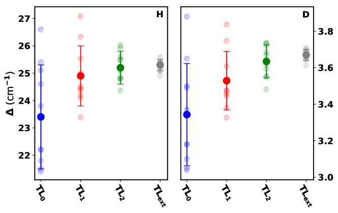Overall, addition of 50 to 100 additional points from the HL treatment appears to suffice to arrive at a quantitatively correct PES transfer-learned from the LL treatment (MP2/aug-cc-pVTZ). Figure 3 illustrates the gradual convergence for TL₀ to TL₂ towards the results found for TL_ext, which is promising. While exceptional agreement regarding the energy barrier $E_{\mathrm{B}}$ (as the “simpler” property) is found for all the TLs the standard deviation of the splittings $\Delta_{\rm H}$ (which is more challenging to obtain) can be reduced from 1.9 cm^-1 (7.5%) for TL₀ to 0.5 cm^-1 (2%) for TL₂. The results from TL₂ are accurate to within 0.1 cm^-1 for HT and 0.04 cm^-1 for DT as compared to ${\rm TL}_{\rm ext}$. This corresponds to deviations of 0.4% and 1.1%. The IPs themselves are reported in Figures S1 to S4 and show slight deviations between the different TLs on the smallest data set (TL₀), but for TL₁, TL₂ and TL_ext they are hardly distinguishable.

In summary, it has been found that with between 25 and 50 HL energies and forces for judiciously chosen structures the correct barrier height, tunneling splitting, action and fluctuation can be obtained, see Table 1. This is the foundation to further optimize the procedure, ideally based entirely on information available from the LL surface by minimizing the amount of data required from the HL treatment.

3.3 Towards an Optimized Procedure

For an even more efficient procedure, an approach is sought that is based on information about the LL-PES only. Hence, an attempt is made to further reduce the computational effort by minimizing the number of structures for which HL calculations need to be carried out for an improved PES and tunneling splittings. Therefore, it is explored which elements of the procedure are most important for obtaining high accuracy to cost ratios. For moving towards a more evidence-guided, optimized procedure, TL is carried out from LL-information that is only contained in the MEP and IP as follows: a) only the MEP (TL_MEP) using 111 geometries along the MEP of the PhysNet MP2 PES; b) only the IP (TL_IP) using 110 geometries along the IP of the PhysNet MP2 PES; and c) a combination of the MEP and the IP (TL_MI) including 111 MEP and 110 instanton geometries as obtained from the PhysNet MP2 PES. The HL information for TL consisted again of energies, forces and dipole moment determined at the CCSD(T)/aug-cc-pVTZ level of theory. A total of 5 TLs were performed, each on different splits of the data. The two best NNs (judged from the performance on the validation set) were used for further analysis.

	$E_{\mathrm{B}}$ [kcal/mol]	$\Delta_{\rm H}$ [cm-1]	$S/\hbar$	$\Phi$
TL${}_{\rm MEP}^{a}$	3.94	15.4	5.887	76.482
TL${}_{\rm MEP}^{b}$	3.95	14.1	5.912	81.921
TL${}_{\rm IP}^{a}$	3.49	16.7	5.792	76.975
TL${}_{\rm IP}^{b}$	3.50	16.9	5.794	75.858
TL${}_{\rm MI}^{a}$	3.90	18.2	5.768	72.262
TL${}_{\rm MI}^{b}$	3.90	16.9	5.774	77.374
$\langle{\rm TL}_{\rm ext}\rangle$	3.8945	25.3	5.743	53.241

Table 2: Energy barriers $E_{\mathrm{B}}$, tunneling splittings $\Delta_{\rm H}$ (at $T=25$ K and $N=4096$), action $S/\hbar$ and fluctuation factor $\Phi$ (in a.u. of time $\hbar/E_{h}$) for HT determined from TL PESs using MEP points only (TL_MEP), instanton points only (TL_IP), and a combination of MEP and instanton points (TL_MI). TL${}_{\rm x}^{a}$ and TL${}_{\rm x}^{b}$ correspond to two NNs that are trained on different splits of the data. Note that the energy barrier for TL_IP is inaccurate, as expected, because the IP misses the transition state of the PES. The ab initio barrier at the CCSD(T)/aug-cc-pVTZ level of theory is 3.8948 kcal/mol.

First, it is noted that for TL_MEP and TL_MI the barrier $E_{\mathrm{B}}$ for HT agrees well with the target value of 3.8948 kcal/mol (ab initio CCSD(T)/aug-cc-pVTZ level value) whereas this is not the case for TL_IP, as expected, because the instanton path does not pass through the transition state of the MEP (see Table 2). Also, despite starting from MP2 information only, TL to the HL model yields considerably improved tunneling splittings $\Delta_{\rm H}$ for all three models, ranging from 15 to 18 cm^-1, compared to those from the PhysNet MP2 PES (96 cm^-1).

Considering the action $S/\hbar$ from TL_MEP, TL_IP and TL_MI it is seen that it progressively approaches that from TL_ext. For TL_MEP the action overshoots the target value from TL_ext by $\sim 0.15$ which leads to an error of $\sim 15$ % in the splitting because $S/\hbar$ appears in the exponential factor in Eq. 1. Conversely, with a difference of 0.04 compared with TL_ext, the error for TL_MI due to $S/\hbar$ is only $\sim 4$ %. The influence of $\Phi$ on the difference between TL_ext and the three models considered in Table 2 is minor because for all of them $\Phi$ is uniformly too large by $\sim 40$ % compared with that from TL_ext.

Table 2 suggests that a combination of information from the MEP and the IP used for transfer learning, i.e. TL_MI, yields $E_{\rm B}$ and $\Delta_{\rm H}$ closest to the results from TL_ext. However, the tunneling splittings still differ by more than 10 % from the target value obtained on the TL_ext PESs. Considering the actions $S/\hbar$ and fluctuations $\Phi$ for all the transfer learned PESs in Table 2 it is found that in particular the values of $\Phi$, which are sensitive to fluctuations around the IP, differ considerably from that on TL_ext. Hence as a last improvement points along the MEP and IP are combined with structures around the IP.

	$N_{\rm data}$	$E_{\rm B}$	$\Delta_{\rm H}$	$S/\hbar$	$\Phi$
MP2	70k	2.7889	96.3	4.502	42.770
$\langle{\rm TL}_{0}\rangle$	25	$3.8925\pm 0.0119$	$23.4\pm 1.9$	$5.749\pm 0.026$	$57.405\pm 4.486$
$\langle{\rm TL}_{1}\rangle$	50	$3.8974\pm 0.0161$	$24.9\pm 1.1$	$5.764\pm 0.01$2	$53.096\pm 2.375$
$\langle{\rm TL}_{2}\rangle$	100	$3.8941\pm 0.0021$	$25.2\pm 0.5$	$5.748\pm 0.005$	$53.053\pm 1.156$
$\langle{\rm TL}_{\rm ext}\rangle$	862	$3.8945\pm 0.0006$	$25.3\pm 0.2$	$5.743\pm 0.002$	$53.241\pm 0.454$
$\langle{\rm TL}_{\rm EB1}\rangle$	25	$3.9025\pm 0.0232$	$23.7\pm 1.1$	$5.740\pm 0.013$	$57.099\pm 3.249$
$\langle{\rm TL}_{\rm EB2}\rangle$	25	$3.9041\pm 0.0189$	$23.5\pm 2.1$	$5.733\pm 0.025$	$58.241\pm 4.850$

Table 3: Energy barriers $E_{\mathrm{B}}$ (kcal/mol), tunneling splittings $\Delta_{\rm H}$ (in cm^-1) at $T=25$ K and with $N=4096$, action $S/\hbar$ and fluctuation factor $\Phi$ (in a.u. of time $\hbar/E_{h}$) for malonaldehyde determined from TL_EB. The ab initio barrier at the CCSD(T)/aug-cc-pVTZ level of theory is 3.8948 kcal/mol.

For two final, evidence-based TLs (TL_EB1 and TL_EB2), a set of 25 data points was generated as follows. A total of 5 points was selected along the MEP and IP (one close to the minimum and 2 points along the PhysNet MP2 PES MEP and IP each, see black points in Figure 5). These were supplemented by 20 geometries from NMS around the equilibrium structure and the IP that are selected by means of an RMSD criterion. For TL_EB1 (orange circles in Figure 5), the geometries with largest RMSD are selected (single geometries which occupy the same $r_{\rm OO}$ and $q$ coordinates are eliminated). For TL_EB2 (green crosses in Figure 5), besides the RMSD criterion, the geometries were selected to cover the important configurational space more regularly (as judged by Figure 5).

For both sets of points the corresponding CCSD(T)/aug-cc-pVTZ energies, forces and dipole moments were used for TL, resulting in two sets of transfer learned PESs: TL_EB1 and TL_EB2. For both of them the barrier height (3.90 kcal/mol) is within error bars of TL_ext for which it was 3.89 kcal/mol. The action $S/\hbar$ for both EB-models agree with TL_ext within error bounds although the fluctuations around the mean is larger by almost an order of magnitude, see Table 3. For the fluctuation $\Phi$ the differences compared with TL_ext are $\sim 5$ %, commensurate with TL₀ and evidently improved over those using MEP, IP or MI, see Table 2 which do not train on geometries around the path. The tunneling splittings are $\Delta_{\rm H,EB1}=23.7\pm 1.1$ cm^-1 and $\Delta_{\rm H,EB2}=23.5\pm 2.1$ cm^-1, both of which are close to/within error bounds of the reference value $(25.3\pm 0.2)$, see Table 3. These results are comparable and slightly better to those on TL₀ which also was based on only 25 points for TL. However, the training data for TL_EB1,EB2 are selected based entirely on the PhysNet MP2 PES whereas TL₀ made use of HL information in that it employed geometries along the IP of a PES with corrected barrier. Hence, from a computational perspective, the EB models are considerably more cost-effective.

Figure 5: The data sets used for TL_EB1 (orange circles) and TL_EB2 (green crosses) are shown on a 2D projection of the PES spanned by the O–O distance and the reaction coordinate $q=r_{\rm O_{A}H}-r_{\rm O_{B}H}$. Both data set contain 25 geometries. The MEP and the IP (as determined on the TL_ext PES) are marked with a dash-dotted and a dashed line, respectively. The IP on the MP2 PES is illustrated as white dashed line.

Overall, it is found that TL to the HL with 25 additional points yields a barrier height that agrees with the full HL treatment and the tunneling splitting differs by only $\sim 1$ cm^-1. Any further improvement requires additional points. Based on the results in Table 3 it is expected that using a TL model trained on fewer than 50 judiciously selected HL data points yields results within 1% of the HL reference TL_ext. This needs also be contrasted with an expected accuracy of instanton calculations for tunneling splittings of $\sim 20$ %.

4 Discussion and Conclusions

The present work aimed at developing a computationally efficient and accurate road-map for how to improve a given LL model - which was assumed to be “comprehensive” (here $7\times 10^{4}$ MP2 energies and forces were used) for the observable of interest - to a HL model by providing a small amount of additional information at the higher level of theory considering a particular observable. Here, the observable was the tunneling splitting for HT/DT in malonaldehyde for which the LL model (MP2/aug-cc-pVTZ) yielded $\Delta=96$ cm^-1, compared with a literature value of $\Delta_{\rm H}\sim 25$ cm^-1 from a PIP-represented PES of CCSD(T)/aug-cc-pVTZ reference energies using a range of methods for computing $\Delta_{\rm H/D}$, see Table S7. Most HL models generated were based on TL using 10s to 100s of HL points and yield $\Delta\sim 25$ cm^-1 which is a substantial improvement over the LL model and consistent with computations in the literature at the same level of theory but employing computationally much more demanding approaches. The remaining differences between computations and experiments are due to a) shortcomings of the CCSD(T) level of theory compared with a full CI treatment, b) the incompleteness of the basis set, and c) inherent semiclassical approximations of instanton theory (e.g. neglect of coupling to overall molecule rotation and anharmonicity perpendicular to the instanton path).

A typically used shortcut is to optimize the instanton using a LL ab initio method, e.g. DFT or MP2, and then compute the CCSD(T) properties along the path to correct the action $S/\hbar$. Such a hybrid approach was assessed using the PhysNet MP2 PES to optimize the instanton and then calculate the action $S/\hbar$ on the TL_ext PES.^{11, 50, 12, 51} The results are summarized in Table 4 and illustrate that although the hybrid approach is, in this case, able to infer the correct value for $S/\hbar$, the TL approach additionally improves $\Phi$. Using Equation 1 with the action as determined by the hybrid approach ($S/\hbar=5.7401$) and the fluctuation factor determined on the PhysNet MP2 PES ($\Phi=42.7705$) yields $\Delta_{\rm H}\sim 31.5$ cm^-1 which overestimates the value of 25.1 cm^-1 from TL_ext. The TL approach is thus able to provide a more accurate prediction of $\Delta$ for a similar computational cost.

	H			D
PES	$\Delta_{\rm H}$	$S/\hbar$	$\Phi$	$\Delta_{\rm D}$	$S/\hbar$	$\Phi$
MP2	96.3	4.502	42.771	18.8	5.705	73.964
Hybrid	31.5	5.740	42.771	4.4	7.276	73.964
$\langle{\rm TL}_{\rm EB2}\rangle$	23.5	5.733	58.241	3.5	7.266	94.777
TLext	25.1	5.744	53.586	3.6	7.274	89.957
$\langle{\rm TL}_{\rm ext}\rangle$	25.3	5.743	53.241	3.7	7.273	89.350
Lit.6	25	6.129	37.794	3.3	7.790	61.392

Table 4: Actions $S/\hbar$ and fluctuation factor $\Phi$ as obtained from the MP2 PhysNet PES (MP2), on a representative TL_ext PES (TL_ext) and a hybrid approach optimizing the IP on the PhysNet MP2 PES and using TL_ext to obtain CCSD(T) properties along resulting IP⁶

Mode	MP2	$\langle{\rm TL}_{0}\rangle$	$\langle{\rm TL}_{1}\rangle$	$\langle{\rm TL}_{2}\rangle$	$\langle{\rm TL}_{\rm EB1}\rangle$	$\langle{\rm TL}_{\rm ext}\rangle$	CCSD(T)
1	277.49	266.68	265.48	265.28	266.93	265.17	264.71
2	286.59	285.58	283.96	280.88	286.01	283.77	281.85
3	394.33	389.41	387.06	389.09	392.05	389.70	389.12
4	514.07	501.82	502.93	503.23	505.62	505.50	505.07
5	789.38	772.93	774.86	775.82	773.14	775.33	775.06
6	888.62	885.17	886.17	886.92	885.18	886.39	886.07
7	937.61	906.84	907.54	908.64	908.10	908.03	907.18
8	1012.29	988.09	989.05	992.64	991.79	990.78	989.73
9	1023.82	1005.95	1004.01	1002.71	1006.17	1002.93	1002.60
10	1048.75	1039.62	1039.69	1038.19	1039.50	1037.56	1037.85
11	1109.69	1104.46	1104.81	1102.64	1102.08	1102.20	1101.03
12	1288.28	1274.86	1271.94	1272.65	1272.27	1273.41	1272.73
13	1403.09	1400.18	1399.97	1401.56	1402.15	1401.73	1400.73
14	1407.97	1404.80	1408.40	1407.17	1406.59	1408.81	1406.94
15	1482.06	1458.89	1463.84	1463.95	1462.21	1467.70	1469.33
16	1641.52	1624.37	1627.95	1630.14	1631.91	1633.35	1632.52
17	1692.91	1681.91	1687.06	1691.27	1686.72	1693.59	1693.63
18	3039.02	3003.37	2999.68	2999.67	3005.82	3000.03	3001.26
19	3107.12	3176.46	3178.76	3180.11	3176.23	3176.74	3176.35
20	3217.85	3229.25	3228.54	3228.74	3232.47	3226.75	3227.12
21	3267.30	3259.40	3260.39	3262.98	3254.33	3263.25	3260.27
MAE	14.62	3.01	1.93	1.54	2.61	0.89

Table 5: Averaged harmonic frequencies calculated from PhysNet potentials and using ab initio techniques are given in cm^-1. As judged from the MAE($\omega$) the PhysNet model trained on the Extended Data Set containing 862 geometries is the most accurate, followed by the TL₂ (100 data points), TL₁ (50 data points) TL_EB1 (25 data points) and TL₀ (25 data points). The ab initio harmonic frequencies obtained at the MP2 level are shown for comparison.

For calculating the tunneling splittings based on the instanton approach it was found that an evidence-based approach starting from MEP and IP on the LL PES, augmented with geometries drawn from a pool of structures selected such that their RMSD is maximal with respect to an existing set of structures requires of the order of 50 points at the HL for TL. Therefore, only local and not global knowledge of the PES is required as would, e.g. be necessary for fully quantum-mechanical methods such as wavepackets. The bottleneck to a “direct” ab initio-based instanton approach is typically the calculation of $N$ Hessians, as these are rather expensive to compute.^{11, 12} Earlier work on instanton rate theory combined with machine-learning techniques for the H + CH₄ and H + C₂H₆ reactions required $\sim 50$ energies and forces and 8 Hessians in the training set to converge the rate constant to within $1$ % of the ab initio result at 200 K.¹³ Using TL, calculating any high-level ab initio Hessians at all has been avoided. As is demonstrated here, this can significantly lower the computational expense with no loss of accuracy.

With regards to the accuracy of the TL PESs it is of interest to compare their performance on out-of-sample structures. For this a test set was generated from MD simulations at 700 K on one of the TL_ext PESs from which 100 geometries were randomly extracted. In addition, 10 equally spaced off-grid geometries along the IP on the same PES were selected. The CCSD(T)/aug-cc-pVTZ energies of these 110 geometries cover a range from $\sim 5$ to $40$ kcal/mol above the global minimum. The energies for these structures were computed based on TL_ext (most rigorous TL using 862 HL structures) and TL_EB1 (following the recommended procedure; TL with 25 HL energies and forces), respectively, and the [MAE₁₀₀($E$),MAE₁₀($E$)] for the two out-of-sample sets are [0.21,0.004] kcal/mol and [0.34,0.005] kcal/mol. Notably, the energies of the geometries used for TL_ext and TL_EB1 only cover a range 20 kcal/mol above the global minimum whereas the out-of-sample energies reach twice as high, up to 40 kcal/mol above the minimum. Hence, the out-of-sample structures contain true predictions on the HL-PES. As a comparison, for the PIP PES, which used energies only and no forces, the reported fitting errors (i.e. in-sample) are 32 cm^-1 (0.09 kcal/mol) for energies below 2000 cm^-1 (5.7 kcal/mol) above the global minimum and 211 cm^-1 (0.6 kcal/mol) for energies up to 20000 cm^-1 (51.2 kcal/mol).²⁹

TL as used in the present work - namely as a local refinement of a LL-PES - can also be regarded as a variant of the more global “morphing” approach for PESs.⁵² It is therefore of interest to consider in what way observables other than the tunneling splitting change upon TL from LL to HL. For this, harmonic frequencies were determined for a number of transfer learned PESs. The harmonic frequencies averaged over the 10 individually trained NNs for different TLs are reported in Table 5, where they are compared with frequencies determined from CCSD(T)/aug-cc-pVTZ calculations at the corresponding equilibrium structure of malonaldehyde. As judged from the MAE($\omega$) the PhysNet model for TL_ext is most accurate (MAE $<1$ cm^-1), followed by TL₂ (MAE $<2$ cm^-1), TL₁ (MAE $\sim 2$ cm^-1)and TL₀ (MAE $\sim 3$ cm^-1), as expected, and show a considerable improvement over the MP2 frequencies. For TL_EB1 the MAE is $<3$ cm^-1. Thus, TL to the HL model also improves the shape of the PES in degrees orthogonal to the two reaction coordinates considered for the tunneling splitting.

Figure 6: Flowchart of the recommended TL + RPI procedure.

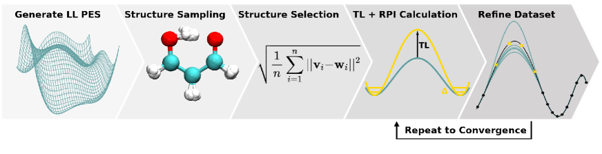
In terms of a recommended procedure it is noted that the strategy outlined in going from TL₁ to TL₂ (adaptive sampling/active learning) can also be pursued recursively from a “pool” of geometries generated from sampling the PhysNet MP2 PES. This procedure can be repeated until convergence of the barrier height and the tunneling splittings. The approach proposed for future application is (see Figure 6): i) create a LL-PES from a fine grid (here $7\times 10^{4}$ points) and train a ML model (here PhysNet) ii) generate a pool of structures based on the LL-PES (including MEP, Instanton, NMS) iii) choose $N\sim 25$ geometries following EB1/2 and determine energies and forces from HL ab initio calculations iv) perform TL and instanton calculations on the HL-PES v) refine the data set using adaptive sampling and structures along the new IP. Then repeat TL and instanton calculations vi) repeat iv) and v) until convergence. The present work demonstrates that following such a road-map requires $\sim 50$ HL energy and force evaluations to determine an accurate tunneling splitting of malonaldehyde which is manifestly more efficient than previously explored approaches.

In summary, given that LL models can be constructed efficiently even for moderately sized molecules such as malonaldehyde or larger,⁵³ the present work confirms that with specific, evidence-based information grounded in physical understanding of the process in question, several 10 points from a HL treatment are sufficient to generate high-quality PESs for a target observable which was the tunneling splitting in malonaldehyde in the present work. The MAE($E$) for the TL-PESs trained on energies spanning 20 kcal/mol above the global minimum is $\sim 0.3$ kcal/mol on off-grid structures spanning 40 kcal/mol and the resulting harmonic frequencies agree to within 1 to 3 cm^-1 with rigorous and very time consuming normal mode analysis at the CCSD(T)/aug-cc-pVTZ level of theory. The recommended approach deduced from the present work is based on information about the MEP, the IP, and fluctuations around the IP determined on the LL-PES for which HL calculations are required for TL to determine the HL-PES. It is expected that - with suitable adaptations due to the particular observable considered - the present approach can also be applied to other observables that are computationally expensive to determine for a given PES, e.g. the quantum bound states of molecules or scattering cross sections for gas phase reactions from wavepacket propagation.

References

- Richardson and Althorpe 2011 Richardson, J. O.; Althorpe, S. C. Ring-polymer instanton method for calculating tunneling splittings. J. Chem. Phys. 2011, 134, 054109
- Richardson 2018 Richardson, J. O. Ring-polymer instanton theory. Int. Rev. Phys. Chem. 2018, 37, 171–216
- Richardson et al. 2016 Richardson, J. O.; Pérez, C.; Lobsiger, S.; Reid, A. A.; Temelso, B.; Shields, G. C.; Kisiel, Z.; Wales, D. J.; Pate, B. H.; Althorpe, S. C. Concerted Hydrogen-Bond Breaking by Quantum Tunneling in the Water Hexamer Prism. Science 2016, 351, 1310–1313
- Richardson 2017 Richardson, J. O. Full-and reduced-dimensionality instanton calculations of the tunnelling splitting in the formic acid dimer. Phys. Chem. Chem. Phys. 2017, 19, 966–970
- Coleman 1977 Coleman, S. The uses of instantons. 1977; Also in S. Coleman, Aspects of Symmetry, chapter 7, pp. 265–350 (Cambridge University Press, 1985)
- Jahr et al. 2020 Jahr, E.; Laude, G.; Richardson, J. O. Instanton theory of tunneling in molecules with asymmetric isotopic substitutions. J. Chem. Phys. 2020, 153, 094101
- Hammer and Manthe 2011 Hammer, T.; Manthe, U. Intramolecular proton transfer in malonaldehyde: Accurate multilayer multi-configurational time-dependent Hartree calculations. J. Chem. Phys. 2011, 134, 224305
- Schröder et al. 2011 Schröder, M.; Gatti, F.; Meyer, H.-D. Theoretical studies of the tunneling splitting of malonaldehyde using the multiconfiguration time-dependent Hartree approach. J. Chem. Phys. 2011, 134, 234307
- Mátyus et al. 2016 Mátyus, E.; Wales, D. J.; Althorpe, S. C. Quantum tunneling splittings from path-integral molecular dynamics. J. Chem. Phys. 2016, 144, 114108
- Vaillant et al. 2018 Vaillant, C. L.; Wales, D. J.; Althorpe, S. C. Tunneling splittings from path-integral molecular dynamics using a Langevin thermostat. J. Chem. Phys. 2018, 148, 234102
- Mil’nikov et al. 2003 Mil’nikov, G. V.; Yagi, K.; Taketsugu, T.; Nakamura, H.; Hirao, K. Tunneling splitting in polyatomic molecules: Application to malonaldehyde. J. Chem. Phys. 2003, 119, 10–13
- Sahu et al. 2021 Sahu, N.; Richardson, J. O.; Berger, R. Instanton calculations of tunneling splittings in chiral molecules. J. Comput. Chem. 2021, 42, 210–221
- Laude et al. 2018 Laude, G.; Calderini, D.; Tew, D. P.; Richardson, J. O. Ab initio instanton rate theory made efficient using Gaussian process regression. Faraday Discuss. 2018, 212, 237–258
- Cooper et al. 2018 Cooper, A. M.; Hallmen, P. P.; Kästner, J. Potential energy surface interpolation with neural networks for instanton rate calculations. J. Chem. Phys. 2018, 148, 094106
- McConnell and Kästner 2019 McConnell, S. R.; Kästner, J. Instanton rate constant calculations using interpolated potential energy surfaces in nonredundant, rotationally and translationally invariant coordinates. J. Comput. Chem. 2019, 40, 866–874
- Unke et al. 2020 Unke, O. T.; Koner, D.; Patra, S.; Käser, S.; Meuwly, M. High-dimensional potential energy surfaces for molecular simulations: from empiricism to machine learning. Mach. learn.: sci. technol. 2020, 1, 013001
- Friesner 2005 Friesner, R. A. Ab initio quantum chemistry: Methodology and applications. Proc. Natl. Acad. Sci. USA 2005, 102, 6648–6653
- Pan and Yang 2009 Pan, S. J.; Yang, Q. A survey on transfer learning. IEEE Trans. Knowl. Data Eng. 2009, 22, 1345–1359
- Taylor and Stone 2009 Taylor, M. E.; Stone, P. Transfer learning for reinforcement learning domains: A survey. J. Mach. Learn. Res. 2009, 10, 1633–1685
- Smith et al. 2019 Smith, J. S.; Nebgen, B. T.; Zubatyuk, R.; Lubbers, N.; Devereux, C.; Barros, K.; Tretiak, S.; Isayev, O.; Roitberg, A. E. Approaching coupled cluster accuracy with a general-purpose neural network potential through transfer learning. Nat. Commun. 2019, 10, 1–8
- Ramakrishnan et al. 2015 Ramakrishnan, R.; Dral, P.; Rupp, M.; von Lilienfeld, O. A. Big Data meets quantum chemistry approximations: The -machine learning approach. J. Chem. Theory Comput. 2015, 11, 2087–2096
- Käser et al. 2020 Käser, S.; Unke, O. T.; Meuwly, M. Reactive dynamics and spectroscopy of hydrogen transfer from neural network-based reactive potential energy surfaces. New J. Phys. 2020, 22, 055002
- Käser et al. 2020 Käser, S.; Koner, D.; Christensen, A. S.; von Lilienfeld, O. A.; Meuwly, M. Machine Learning Models of Vibrating H2CO: Comparing Reproducing Kernels, FCHL, and PhysNet. J. Phys. Chem. A 2020, 124, 8853–8865
- Nandi et al. 2021 Nandi, A.; Qu, C.; Houston, P. L.; Conte, R.; Bowman, J. M. -machine learning for potential energy surfaces: A PIP approach to bring a DFT-based PES to CCSD(T) level of theory. J. Chem. Phys. 2021, 154, 051102
- Käser et al. 2021 Käser, S.; Boittier, E. D.; Upadhyay, M.; Meuwly, M. Transfer Learning to CCSD(T): Accurate Anharmonic Frequencies from Machine Learning Models. J. Chem. Theory Comput. 2021, 17, 3687–3699
- Qu et al. 2021 Qu, C.; Houston, P. L.; Conte, R.; Nandi, A.; Bowman, J. M. Breaking the Coupled Cluster Barrier for Machine-Learned Potentials of Large Molecules: The Case of 15-Atom Acetylacetone. J. Phys. Chem. Lett. 2021, 12, 4902–4909
- Käser and Meuwly 2022 Käser, S.; Meuwly, M. Transfer learned potential energy surfaces: accurate anharmonic vibrational dynamics and dissociation energies for the formic acid monomer and dimer. Phys. Chem. Chem. Phys. 2022, 24, 5269–5281
- Laude et al. 2020 Laude, G.; Calderini, D.; Welsch, R.; Richardson, J. O. Calculations of quantum tunnelling rates for Muonium reactions with methane, ethane and propane. Phys. Chem. Chem. Phys. 2020, 22, 16843–16854
- Wang et al. 2008 Wang, Y.; Braams, B. J.; Bowman, J. M.; Carter, S.; Tew, D. P. Full-dimensional quantum calculations of ground-state tunneling splitting of malonaldehyde using an accurate ab initio potential energy surface. J. Chem. Phys. 2008, 128, 224314
- Cvitas and Althorpe 2016 Cvitas, M. T.; Althorpe, S. C. Locating instantons in calculations of tunneling splittings: The test case of malonaldehyde. J. Chem. Theory Comput. 2016, 12, 787–803
- Mizukami et al. 2014 Mizukami, W.; Habershon, S.; Tew, D. P. A compact and accurate semi-global potential energy surface for malonaldehyde from constrained least squares regression. J. Chem. Phys. 2014, 141, 144310
- Firth et al. 1991 Firth, D.; Beyer, K.; Dvorak, M.; Reeve, S.; Grushow, A.; Leopold, K. Tunable far-infrared spectroscopy of malonaldehyde. J. Chem. Phys. 1991, 94, 1812–1819
- Baba et al. 1999 Baba, T.; Tanaka, T.; Morino, I.; Yamada, K. M.; Tanaka, K. Detection of the tunneling-rotation transitions of malonaldehyde in the submillimeter-wave region. J. Chem. Phys. 1999, 110, 4131–4133
- Redington et al. 2008 Redington, R. L.; Redington, T. E.; Sams, R. L. Infrared Absorption Spectra in the Hydroxyl Stretching Regions of Gaseous Tropolone OHO Isotopomers. Z. Phys. Chem. 2008, 222, 1197–1211
- Murdock et al. 2010 Murdock, D.; Burns, L. A.; Vaccaro, P. H. Vibrational specificity of proton-transfer dynamics in ground-state tropolone. Phys. Chem. Chem. Phys. 2010, 12, 8285–8299
- Ortlieb and Havenith 2007 Ortlieb, M.; Havenith, M. Proton transfer in (HCOOH)2: an IR high-resolution spectroscopic study of the antisymmetric C–O stretch. J. Phys. Chem. A 2007, 111, 7355–7363
- Zhang et al. 2017 Zhang, Y.; Li, W.; Luo, W.; Zhu, Y.; Duan, C. High resolution jet-cooled infrared absorption spectra of (HCOOH)2,(HCOOD)2, and HCOOH-HCOOD complexes in 7.2 m region. J. Chem. Phys. 2017, 146, 244306
- Li et al. 2019 Li, W.; Evangelisti, L.; Gou, Q.; Caminati, W.; Meyer, R. The barrier to proton transfer in the dimer of formic acid: a pure rotational study. Angew. Chem. Int. Ed. Engl. 2019, 58, 859–865
- Insausti et al. 2022 Insausti, A.; Ma, J.; Yang, Q.; Xie, F.; Xu, Y. Rotational Spectroscopy of 2-Furoic Acid and Its Dimer: Conformational Distribution and Double Proton Tunneling. ChemPhysChem 2022, 23, e202200176
- Baughcum et al. 1984 Baughcum, S. L.; Smith, Z.; Wilson, E. B.; Duerst, R. W. Microwave spectroscopic study of malonaldehyde. 3. Vibration-rotation interaction and one-dimensional model for proton tunneling. J. Am. Chem. Soc. 1984, 106, 2260–2265
- Mil’nikov and Nakamura 2001 Mil’nikov, G. V.; Nakamura, H. Practical implementation of the instanton theory for the ground-state tunneling splitting. J. Chem. Phys. 2001, 115, 6881–6897
- Richardson 2018 Richardson, J. O. Perspective: Ring-polymer instanton theory. J. Chem. Phys. 2018, 148, 200901
- Richardson et al. 2011 Richardson, J. O.; Althorpe, S. C.; Wales, D. J. Instanton calculations of tunneling splittings for water dimer and trimer. J. Chem. Phys. 2011, 135, 124109
- Unke and Meuwly 2019 Unke, O. T.; Meuwly, M. PhysNet: A neural network for predicting energies, forces, dipole moments, and partial charges. J. Chem. Theory Comput. 2019, 15, 3678–3693
- Gilmer et al. 2017 Gilmer, J.; Schoenholz, S. S.; Riley, P. F.; Vinyals, O.; Dahl, G. E. Neural message passing for quantum chemistry. Proc. of the 34th Int. Conf. on Machine Learning-Volume 70. 2017; pp 1263–1272
- Baydin et al. 2017 Baydin, A. G.; Pearlmutter, B. A.; Radul, A. A.; Siskind, J. M. Automatic differentiation in machine learning: a survey. J. Mach. Learn. Res. 2017, 18, 5595–5637
- Abadi et al. 2016 Abadi, M.; Barham, P.; Chen, J.; Chen, Z.; Davis, A.; Dean, J.; Devin, M.; Ghemawat, S.; Irving, G.; Isard, M. et al. Tensorflow: A system for large-scale machine learning. 12th USENIX symposium on operating systems Design and Implementation (OSDI 16). 2016; pp 265–283
- Werner et al. 2019 Werner, H.-J.; Knowles, P. J.; Knizia, G.; Manby, F. R.; Schütz, M.; Celani, P.; Györffy, W.; Kats, D.; Korona, T.; Lindh, R. et al. MOLPRO, version 2019, a package of ab initio programs. 2019
- Behler 2015 Behler, J. Constructing high-dimensional neural network potentials: A tutorial review. Int. J. Quantum. Chem. 2015, 115, 1032–1050
- Meisner and Kästner 2018 Meisner, J.; Kästner, J. Dual-Level Approach to Instanton Theory. J. Chem. Theory Comput. 2018, 14, 1865–1872
- Heller and Richardson 2022 Heller, E. R.; Richardson, J. O. Heavy-Atom Quantum Tunnelling in Spin Crossovers of Nitrenes. Angew. Chem. Int. Ed. 2022,
- Meuwly and Hutson 1999 Meuwly, M.; Hutson, J. Morphing Ab Initio Potentials: A Systematic Study of Ne-HF. J. Chem. Phys. 1999, 110, 8338–8347
- Koner and Meuwly 2020 Koner, D.; Meuwly, M. Permutationally invariant, reproducing kernel-based potential energy surfaces for polyatomic molecules: From formaldehyde to acetone. J. Chem. Theory Comput. 2020, 16, 5474–5484